Ubiquitous Time Variability of Integrated Stellar Populations

Abstract

Long period variable stars arise in the final stages of the asymptotic giant branch phase of stellar evolution. They have periods of up to $\sim 1000$d and amplitudes that can exceed a factor of three in the $I$-band flux. These stars pulsate predominantly in their fundamental mode[1, 2, 3], which is a function of mass and radius, and so the pulsation periods are sensitive to the age of the underlying stellar population[4]. The overall number of long period variables in a population is directly related to their lifetime, which is difficult to predict from first principles because of uncertainties associated with stellar mass-loss and convective mixing. The time variability of these stars has not been previously taken into account when modeling the spectral energy distributions of galaxies. Here we construct time-dependent stellar population models that include the effects of long period variable stars, and report the ubiquitous detection of this expected ‘pixel shimmer’ in the massive metal-rich galaxy M87. The pixel light curves display a variety of behaviors, including linearly rising and falling curves, semi-periodic curves, and sudden increases or decreases in the flux level. The observed variation of $0.1-1$% is very well matched to the predictions of our models. The data provide a strong and novel constraint on the properties of variable stars in an old and metal-rich stellar population, and we infer that the lifetime of long period variables in M87 is shorter by approximately 30% compared to predictions from the latest stellar evolution models.

In typical massive galaxies with $\sim 10^{11}$ stars, the variation in the total light due to long period variables will be small as the summed light curves of many such stars effectively cancel each other out (with random phases the net effect scales as $N^{-1/2}$). If the light is spread out over many (e.g., $\sim 10^{4}-10^{6}$) pixels, then the number of stars per pixel can range from $10^{4}-10^{7}$ and in this regime the number of asymptotic giant branch stars per pixel is small and governed by Poisson statistics. This ‘semi-resolved’ regime is well known[5] and the expected surface brightness fluctuations due to Poisson statistics of rare luminous stars have been observed and studied in several hundred nearby galaxies[6, 7, 8]. We expect in this regime to be able to detect the presence of variable stars through the time dependence of the pixel flux (i.e., the pixel light curve): essentially every pixel is expected to ‘shimmer’ on timescales of several hundred days.

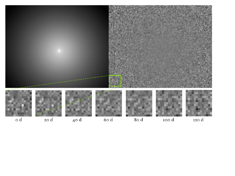
In order to quantify the expected pixel shimmer, we created a stellar population model at solar metallicity that includes the time-dependent effect of long period variables. We started with a new library of stellar isochrones (Choi et al., in prep) that densely samples fast phases of stellar evolution, and assigned periods to evolved stars assuming that they pulsate in the fundamental mode[4]. We then used observations of variable stars in the Galactic bulge from the OGLE survey to estimate a period-amplitude relation in the $I-$band[9, 10, 11]. A smooth surface brightness model of the giant elliptical galaxy M87 was used to specify the luminosity within pixels of size $0.2^{\prime\prime}\times 0.2"$. The pixel luminosity was used to normalize the weights in the isochrone assuming a Salpeter initial mass function[12]. For each pixel the number of giants was drawn from a Poisson distribution and the time evolution of the flux for each giant was given by its associated period and amplitude and initialized with a random phase. An illustration of this time-dependent model for M87 is shown in Fig. 1. The variable star part of our model has a tunable parameter, the long period variable star weight, which can be interpreted as the typical lifetime of such stars. Further details regarding the modeling are provided in the Methods section.

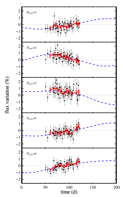
We sampled the model with the same cadence and applied the same photon counting uncertainties as existing observations of M87 (see below). The resulting model pixel light curves are shown in Fig. 2 (blue lines). These pixels were selected to have peak-to-peak flux variation $>1.5$%. While rising and falling curves are clearly seen, one also sees that a $<100$ day observing window can by chance sample a light curve at a phase that appears relatively flat. A $>200$d observing cadence would clearly be ideal for observing the effects of long period variables in the integrated light of nearby galaxies.

To test these expected variations we analyzed archival data of the galaxy M87 from the Hubble Space Telescope collected over 72 days in 2005 [13, 14, 15]. Imaging was obtained in both the F606W and F814W filters with the Advanced Camera for Surveys. We focused our analysis on the F814W imaging as the F606W data were generally of lower quality (both due to a shorter exposure time and the fact that only a single exposure was obtained per visit, which made it difficult to clean the images of blemishes such as hot pixels and cosmic rays). The data were processed via the standard HST pipeline. In total 52 separate images, each with a depth of 1440s, were considered in this analysis. Globular clusters in the field were used to refine the astrometric alignment with subpixel shifts. Accurate subtraction of the background was achieved with several additional corrections to the standard HST pipeline, as detailed in the Methods section. Pixels that deviated by more than 30% from a smooth model of the light profile were masked. This effectively removed all visible globular clusters, background galaxies, the chip gap, and edge effects. We also masked the central region and the well-known jet in M87. The data were binned $4\times 4$ to $0.2^{\prime\prime}\times 0.2^{\prime\prime}$ in order to reduce the spatial coherency imposed by the PSF (note that the models were also spatially binned and have been convolved by the PSF in order to emulate the observations as closely as possible).

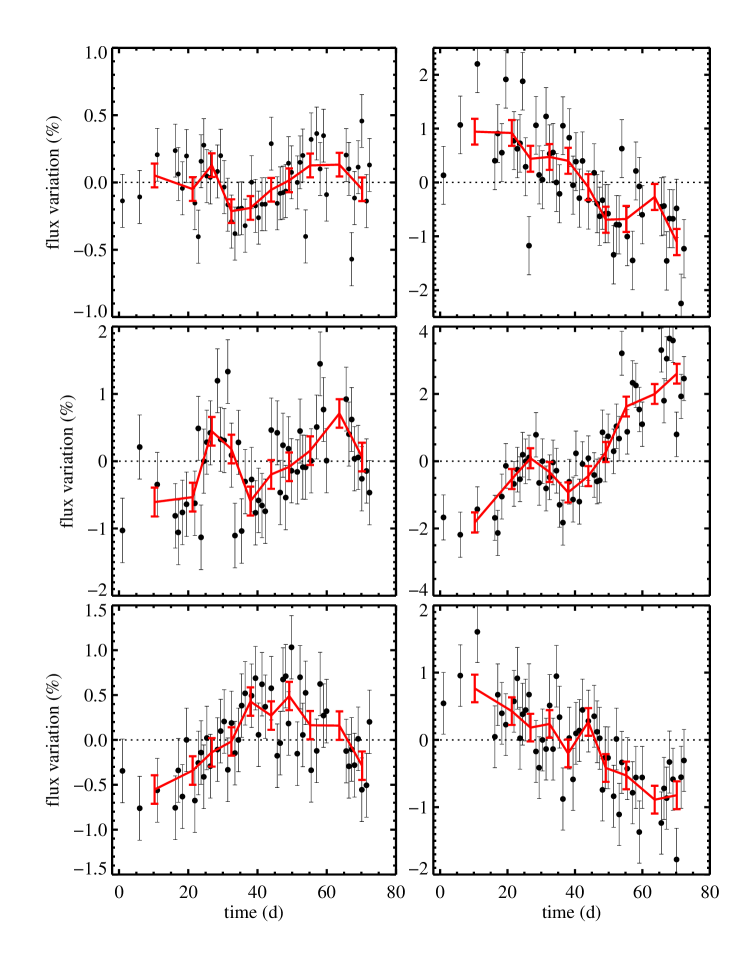
Example pixel light curves for M87 are shown in Fig. 3. The error bars represent photon counting uncertainties only; the solid line is a 5-point boxcar averaging of the data. We detect coherent variation in the pixel light curves that is qualitatively consistent with our model expectations. These examples were chosen to highlight the level of variety seen in the data. We note that a significant fraction of pixel light curves show no evidence of variation within the noise limits of the data. We show below that this is expected if long period variables are the source of the variation.

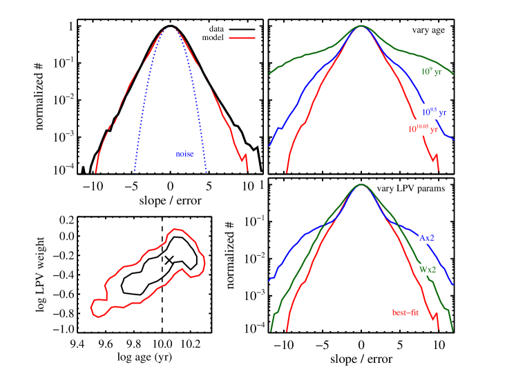
We have quantified the pixel light curves by fitting each curve with a linear function; the best-fit slope and uncertainty were recorded. The resulting distribution of slopes (in units of the uncertainty) is shown in Fig. 4. We find that 24% of pixels (48,100 out of 202,000) show $>2\sigma$ evidence for variation. In our model there are on average 1.5 long period variable stars responsible for variation in each $>2\sigma$ detection. This implies a statistical detection of $\sim 72,000$ variable stars in M87. When averaged over the central $1^{\prime}\times 1^{\prime}$ field of view, the model predicts on average 0.5 variable stars per pixel. In Fig. 4 we compare the observations to the model predictions. We show the sensitivity of the model light curve statistics to both the stellar population age and variable star parameters, and also the posterior probability distributions that result from fitting the model to the observed histogram when allowing the age and relative variable star weight to vary (we do not include the tails of the distribution in the fit as the data are slightly asymmetric beyond $|$slope/err$|\approx 7$). The latter is an overall factor controlling the contribution of variable stars to the integrated light relative to the predictions of a stellar evolution model (see the Methods section for details). The pixel light curves provide a strong constraint on a combination of the age and variable star weight. The dashed line shows the best-fit age estimated from modeling the integrated light spectrum of the central region of M87[16], which allows us to break the degeneracy. It is noteworthy that the best-fit long period variable star weight is less than one, suggesting that such stars in M87 may have shorter lifetimes than current solar metallicity stellar evolution models predict (see the Methods section for a discussion of the effects of metallicity).

This is not the first detection of time variability in the pixel fluxes of nearby galaxies; previous work predicted the occurrence of a gravitational microlensing signal at the pixel level[17], which was subsequently observed[18]. Novae have also been observed in nearby galaxies[19], and indeed we identified $\approx 15$ novae through visual inspection of the pixel light curves for M87. However, novae and microlensing events are rare (though bright) events. An important distinguishing feature of the time variation caused by long period variable stars is the ubiquity — as Fig. 4 shows, 24% of the pixels show $>2\sigma$ evidence for variation.

There are relatively few constraints on the stellar evolutionary phase that gives rise to long period variables. The best constraints to-date on this phase are confined to the Magellanic Clouds, which have sub-solar metallicities characteristic of low mass galaxies. The observations reported here have provided a direct constraint on this important stellar evolutionary phase in a massive, high metallicity galaxy. New stellar evolution models over-predict the lifetimes of long period variables by approximately 30% if one adopts a spectroscopic age for M87 of 10 Gyr. An older mean population age would reduce the mild tension between the models and observations. Constraints such as these on highly evolved, luminous stars are essential for interpreting light from more distant, massive and metal-rich galaxies across the universe.

The detection of time variation in the integrated light of nearby galaxies opens the possibility to derive stellar population ages in these systems by a completely different approach from conventional techniques. In the future, one could imagine high cadence observations of nearby galaxies on $>100$d baselines to detect the period distribution of long period variables by analyzing power spectra of the time series data. This technique is not limited to old stellar systems; on the contrary, younger systems will show considerably greater temporal variation. For example, based on our models, we expect that 4%, 14%, and 22% of pixels with $10^{5}$ stars will show $>1$% absolute flux changes over 100d for ages of $10^{10}$, $10^{9}$, and $10^{8}$ yr, respectively. The larger effect at younger ages is due primarily to the larger fractional contribution of long period variables to the total light (see the Methods section for details). It will therefore be relatively straightforward to perform similar studies on nearby spiral galaxies, where the signal will be much stronger. At a basic and fundamental level, each pixel of a galaxy measurably varies in time, and this variation encodes unique information on its underlying stellar population.

We thank Martin Groenewegen for useful discussions and the referees for comments that improved the quality and clarity of the manuscript. C.C. thanks Brad Holden and Connie Rockosi for asking the question that provided the spark for this paper: “Can one detect Mira variables in integrated light?”

C.C. constructed the models, led the data processing, and contributed to the analysis and interpretation. P.v.D. contributed to the analysis and interpretation. J.C. generated the stellar evolution models and contributed to the analysis and interpretation.

Reprints and permissions information is available at npg.nature.com/reprintsandpermissions. Correspondence and requests for materials should be addressed to C.C. (cconroy@cfa.harvard.edu).

Figure 1: Illustration of pixel shimmer. Model prediction of the effect of long period variables on integrated light. Upper Left: A smooth model for the surface brightness profile of M87. Upper Right: The flux at $t=0$ divided by the mean flux over 1000d within each pixel. Lower panels: Zoom-in on the lower left corner, showing snapshots at 20d intervals. Notice the coherent variation in brightness of individual pixels.

Figure 2: Simulation of pixel light curves. Modeled relative flux variation over 200 days for five random pixels selected to have a peak-to-peak flux variation of $>1.5$%. The underlying stellar population is old and metal-rich and includes long period variable stars. The noise-free model (dashed blue lines) is compared to a simulation of the M87 data, including the photon counting noise ($1\sigma$) and cadence of the observations (symbols), and a boxcar average of the simulated data (red lines). In each panel the number of long period variable stars per pixel with periods $>150$d is indicated in the legend.

Figure 3: Observed pixel light curves for M87. Relative flux variation over 72 days of pixels in M87. We unambiguously detect the ‘pixel shimmer’ due to the contribution of long period variables to the integrated light. These pixels were selected to highlight the variety of morphology of the light curves, including rising, falling, periodic, and peculiar curves. Errors represent $1\sigma$ photon counting uncertainties.

Figure 4: Statistics of the pixel light curves. Distributions of the best-fit linear slope of the pixel light curve in units of the $1\sigma$ uncertainty on the slope. The data are compared to several models including a variable star-free model (labeled “noise” in the upper left panel), and models varying the age, variable star amplitude, and weight. Models with varying age and weight were fit to the observed histogram and the 1 and 2 sigma confidence limits on these parameters are shown in the lower left panel. The cross symbol denotes the best-fit, shown as a red line in the other panels, and the vertical dashed line indicates the best-fit age from fitting the integrated light spectrum. The lower right panel shows the effect of doubling the amplitudes of the long period variables (“Ax2”; blue line) and the weights (“Wx2”; green line).

METHODS

Data reduction and tests. Owing to the small expected amplitude of the time-dependent flux signal for M87, great care was taken to control systematic effects. In this section we describe the details of the data reduction procedure and the additional corrections that were applied to the images.

We began with the publicly available HST images, in which the four dithered exposures per visit were combined and astrometrically aligned, resampled by the drizzling process, and cosmic rays were removed. The public images include flat field corrections and a standard sky subtraction. We used five globular clusters to refine the astrometric alignment via subpixel shifts (using bilinear interpolation). The mean shift was 0.25 pixels (in both x and y directions) in the unbinned images. All of our analysis was performed on images binned $4\times 4$, so these shifts are a tiny fraction of the final pixel size.

Owing to the large angular extent of M87, the standard ACS pipeline is not able to accurately measure the true sky background. We therefore applied a correction to the sky subtraction. We assumed that the true M87 surface brightness profile is that reported by Kormendy[2], which was derived by combining a variety of space and ground-based data. Using this profile, we estimated the sky background in our ACS images by minimizing the residuals between the ACS data and Kormendy’s profile with the sky background, normalization, and a linear color gradient as free parameters (the latter is to account for differences between our F814W filter and Kormendy’s $V$-band profile). This was done separately for each of the 52 images. We refer to this as the primary sky background correction.

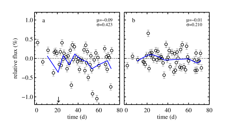
In order to test the fidelity of the images over the 72 days we selected three background galaxies and measured their fluxes within an 8 pixel aperture. These galaxies should show no detectable temporal variation. The resulting temporal variation of the total flux from these galaxies is shown in panel a of Extended Data Fig. 1. There are no obvious time-dependent trends. However the scatter is 0.5%, which is relatively large compared to the signal of interest (of order 1%). We therefore made several additional modifications to the sky background levels in an effort to reduce the scatter.

We identified three additional background galaxies (i.e., not the ones used to measure the flux variation in Extended Data Fig. 1) and measured their flux variation over the duration of the observations. Under the assumption that these sources should have no intrinsic flux variation, we determined a sky background correction necessary to bring the flux of the background galaxies to a constant. The average correction determined this way was 0.002 ct/s. At this point in the analysis the distribution of pixel light curve slopes showed a slight preference for positive slopes (the mean slope/error was +0.5). Under the assumption that the true distribution should have a mean of zero, we subtracted a linearly varying sky background component (which scaled as $5\times 10^{-5}\,t$). These two corrections yield a distribution of pixel light curve slopes with zero mean (by construction), and a temporal flux variation in the three reference background galaxies with a scatter of 0.2% as shown in panel b of Extended Data Fig. 1. Moreover, a 5-point boxcar average of the light curve of the background galaxies shows flux variation at the $\lesssim 0.1$% level. From this test we conclude that it should be possible to measure intrinsic flux variation at the sub percent level, at least for pixels where photon counting noise is not the dominant source of uncertainty.

We emphasize that the additional sky background corrections discussed above do not materially change our conclusions. While these corrections result in a shift in the histogram of slope/err values, they have no effect on the width of the distribution. Moreover, the example pixel light curves shown in Fig. 2 are unchanged within their $1\sigma$ error bars.

Approximately half of the exposures were obtained at a detector location offset by $60-70$ pixels compared to the other half of the exposures. This provides a further test that the trends shown in Fig. 3 and the statistics in Fig. 4 are not dominated by unknown systematics at the level of the detector; if they were, one would have expected to see flux variation that correlated with the dither pattern, but such correlations, if present, are within the noise limits of the data.

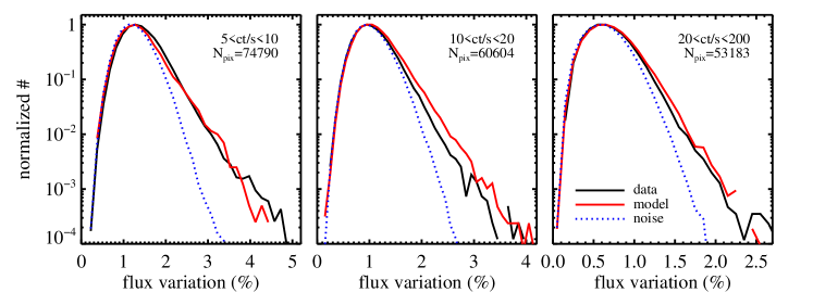
As a final test of both the data reduction and our results, in Extended Data Fig. 2 we show histograms of the flux variation over the 72 day observing window. The flux variation was computed by temporally binning the exposures by five to reduce the Poisson noise in the measurement and computing (max-min)/mean flux at each pixel. The results are shown for three bins of pixel fluxes (the legends show the cuts in units of counts per second and the total number of pixels per bin). The data (black lines) are compared to our best-fit model as derived from fitting the pixel light curve slopes (red lines) and a model without long period variables (blue lines). The good agreement between the model and data in all three panels is a strong indication that our measurements are reliable, as the panels probe a factor of 40 in dynamic range in pixel fluxes. Systematic issues with e.g., the sky subtraction would show up most strongly in the pixels with low count rates, and yet the observations and models agree very well in that regime. Moreover, this flux variation metric is model independent and so the difference between the variable star-free model and the observations provides further strong support that the variation detected in the observations is real and not an artefact of some unknown systematics. There do exist subtle differences between the model and data that vary as a function of the pixel flux, but this could be due to changes in the underlying stellar populations as the pixels with low fluxes are in the outskirts, where the ages and metallicities of the stars are expected to differ from the central regions.

Modeling long period variables. Here we provide additional details regarding the incorporation of long period variables in the stellar population synthesis modeling. We start with stellar isochrones that include all relevant evolutionary phases, including thermally-pulsating asymptotic giant branch (AGB) stars. We include a model for circumstellar dust around these stars, which results in dimmer stars especially for the most intrinsically luminous and evolved stars[3]. Periods (in days) are assigned according to the following equation:

$${\rm log}\,P=-2.07+1.94\,{\rm log}(R/R_{\odot})-0.9\,{\rm log}(M/M_{\odot}),$$ (1)

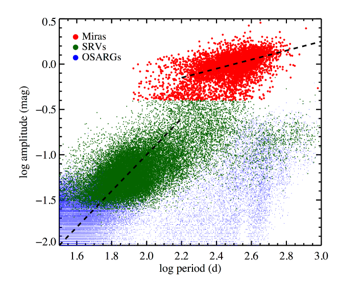
which assumes that the stars pulsate in their fundamental mode[4]. Next, we require a relation between pulsation period and amplitude. This relation is shown in Extended Data Fig. 3 for stars in the Galactic bulge from OGLE data[11]. Symbols are color-coded according to the type of pulsator. The dashed lines are the adopted period-amplitude sequences:

$${\rm log}\,A=0.5\,{\rm log}\,P-1.25,$$ (2)

for the Mira sequence (${\rm log}P>2.2$), and:

$${\rm log}\,A=2\,{\rm log}\,P-5,$$ (3)

for the semi-regular variable (SRV) sequence ($1.0<{\rm log}P<2.2$). In the equations above $P$ is in days and the amplitude $A$ is in the $I-$band in magnitudes. We note that the SRV sequence is included for completeness but has a very small effect on the model predictions.

The equations above, along with the initial mass function weights determined by the masses of the AGB stars in the isochrones, completely specify our default variable star model. In order to convert fluxes to luminosities we have assumed a distance to M87 of 16.7 Mpc[7]. In order to explore the constraining power of the data, we considered variation in both the amplitude of the long period variables, implemented as an overall scaling of all the amplitudes by the same factor, and the weight given to the variable stars in the population synthesis. The latter can be interpreted as a change to the typical lifetime.

We have taken great care to ensure that the long period variable phase is well-resolved in the isochrone tables. The isochrones were constructed from 185 individual mass models and with 600 equivalent evolutionary points in the thermally-pulsating AGB phase alone. We have run a variety of tests to ensure that our model predictions are “converged”; for example we have created models with fewer evolutionary points and fewer input mass models and the resulting predictions are very similar. For context, at 10 Gyr our isochrones contain 350 points on the AGB with periods $>200$d, while the publically available Padova[4] isochrones contain only 3 such points.

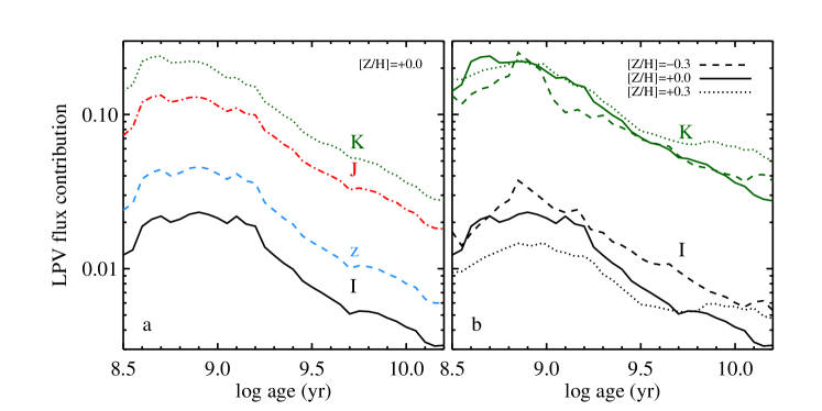
Extended Data Fig. 4 quantifies the fractional contribution of long period variables to the total flux of a stellar population as a function of wavelength, age, and metallicity ([Z/H]). The flux contribution peaks in the age range of $10^{8.5}-10^{9}$ yr and increases toward redder bands. The trend with wavelength is a reflection of the fact that variable stars are cool and so emit most of their light in the near-IR. We caution that the wavelength-dependence shown here does not directly translate into the wavelength-dependence of the time-dependent signal because the period-amplitude relation also depends on wavelength. As the pulsation directly affects the radius and hence the temperature, for these cool stars one expects and indeed observes that the amplitudes are larger in the bluer wavebands[5]. The metallicity-dependence is relatively modest, at least over the range [Z/H]$=-0.3$ to [Z/H]=$+0.3$, typical of massive galaxies. It is difficult to provide a simple explanation of the model metallicity variation, as it depends not only on the variable star lifetime, luminosity, and temperature, but also on the properties of the underlying stellar population.

We do not expect metallicity to play a critical role in the interpretation of the observations for several reasons. First, as noted in the previous paragraph, the models suggest a relatively weak metallicity-dependence of the long period variable flux contribution. Second, M87 harbors a metallicity gradient[6], extending from slightly super-solar in the inner $R_{e}/8$ to slightly sub-solar at $R_{e}$, where $R_{e}$ is the effective radius. Despite this metallicity gradient, our best-fit model provides an equally good fit to the pixel shimmer statistics in both the central region and the outskirts, as shown in Extended Data Fig. 2.

We note here that individual long period variables have been detected in nearby galaxies including the Magellanic Clouds[7], M31[8], and M32[9]. The most distant galaxy with secure detections of individual long period variable stars is NGC 5128[10], and in this case the observations were confined to the outskirts where the stellar density was sufficiently low to permit the separation of the brightest evolved stars from the background sea of lower luminosity stars. These observations of individual long period variables should provide very useful constraints on the modeling of such stars and we intend to make use of these constraints in future work.

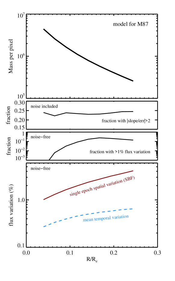
Trends with radius. The HST field of view covers the central $3.3^{\prime}\times 3.3^{\prime}$ of M87, of which the inner $\approx 1^{\prime}\times 1^{\prime}$ has $S/N\gtrsim 100$ per pixel for the observations that were analyzed herein. Kormendy[2] reports an effective radius of $R_{e}=3.2^{\prime}$ so the region of the images with high S/N covers the inner $\approx 0.3R_{e}$. Extended Data Fig. 5 shows several important quantities as a function of $R/R_{e}$ for our best-fit model of M87. Panel a shows the stellar mass per pixel for the underlying smooth stellar distribution. Panel b shows the fraction of pixels with $|$slope/error$|>$2. In the main text we reported that 24% of pixels reach this criterion, and in fact that percentage remains approximately constant with radius. The constancy is the result of two opposing effects: at larger radius the number of stars per pixel is lower, which implies a larger variable star signal. The effect on the slope scales approximately as $\sqrt{N}$ ($N$ being the number of stars per pixel) as multiple variable stars with random phases will cancel each other out in a central limit theorem-like process. However, at larger radius the S/N is lower, and for a fixed exposure time this also scales as $\sqrt{N}$. Thus, for a fixed exposure time, the detectability of long period variables is fairly constant with radius.

The lower two panels of Extended Data Fig. 5 show the model trends with radius for a noise-free model (infinite S/N). In this case it is clear that the absolute effect of long period variables is larger at larger radius. Panel c shows the fraction of pixels with $>1$% peak-to-peak flux variation over 200 d. Old stellar populations with a pixel mass $<10^{6}\,M_{\odot}$ yield $>1$% flux variation in $\sim 10$% of the pixels. Panel d compares the surface brightness fluctuation (SBF) amplitude at a single epoch to the mean temporal variation over a 200 d baseline; the latter is smaller than the former by a factor of $\approx 5$. The SBF amplitude is computed as the standard deviation of the model flux divided by a smooth model for the flux.

We close by noting that while the overall effect of long period variables on the integrated light is relatively modest at old stellar ages, it is much more prominent for younger stellar populations, e.g., in the $10^{8}-10^{9}$ yr range. Future work devoted to younger stellar populations will therefore likely uncover a rich array of observational signatures of time variable stellar populations.

Code Availability We have opted not to make the code used in this manuscript available because the data reduction and analysis is fairly straightforward and can be easily reproduced following the methods described herein.

Figure Extended Data 1: Extended Data Figure 1 $|$ Flux of background galaxies. Time variation of the flux of three background galaxies. The background galaxies should show no intrinsic time variation in their flux and therefore serve as a test of the stability of the data. The mean and standard deviation are reported in each panel. The $1\sigma$ error on each point due to photon counting uncertainty is 0.09%. The solid line is a 5-point boxcar average. a, Flux variation after the standard data reduction including the primary sky background correction. The arrow indicates a point that lies at -2.1. b, Flux variation after additional corrections were applied to the sky background levels. These additional corrections allow us to achieve a stability of $\approx 0.1$% for boxcar averaged time series data.

Figure Extended Data 2: Extended Data Figure 2 $|$ Flux variation distributions. Distribution of (max-min)/mean fluxes over the 72 observing window, separated into three flux bins. The data (black lines) are compared to the best-fit model (red lines) and a noise-only model (blue lines).

Figure Extended Data 3: Extended Data Figure 3 $|$ Amplitude vs. period for luminous variable stars. Data are for Galactic bulge stars from the OGLE survey[11] measured in the $I-$band. Lines are the adopted sequences for Miras and semi-regular variables (SRVs); these relations are used to assign pulsation amplitudes in our model. OGLE small amplitude red giants (OSARGs) are shown for completeness.

Figure Extended Data 4: Extended Data Figure 4 $|$ Long period variable star flux contribution versus age, wavelength, and metallicity. a, Fractional contribution to the total luminosity vs. age in four bandpasses from $I$ ($0.8\mu m$) through $K$ ($2.4\mu m$). The flux contribution scales approximately as $t^{-1/2}$. b, Flux contribution vs. age and metallicity for the $I$ and $K$ bandpasses.

Figure Extended Data 5: Extended Data Figure 5 $|$ Radial variation of model properties for M87. a, Stellar mass per pixel for the smooth underlying model for M87 as a function of $R/R_{e}$ where $R_{e}$ is the effective radius. b, Fraction of pixels with $|$slope/err$|>2$. c, Fraction of pixels in a noise-free model with $>1$% peak-to-peak flux variation over 200 days d, Strength of SBF signal at a single epoch compared to the mean temporal variation due to variable stars in a noise-free model.

References

- [1] Fox, M. W. & Wood, P. R. Theoretical growth rates, periods, and pulsation constants for long-period variables Astrophys. J. 259, 198–212 (1982)
- [2] Wood, P. R. & Sebo, K. M. On the pulsation mode of Mira variables: evidence from the Large Magellanic Cloud Mon. Not. R. Astron. Soc. 282, 958–964 (1996)
- [3] Ita, Y. et al. Variable stars in the Magellanic Clouds - II. The data and infrared properties Mon. Not. R. Astron. Soc. 353, 705–712 (2004)
- [4] Vassiliadis, E. & Wood, P. R. Evolution of low- and intermediate-mass stars to the end of the asymptotic giant branch with mass loss Astrophys. J. 413, 641–657 (1993)
- [5] Tonry, J. & Schneider, D. P. A new technique for measuring extragalactic distances Astronom. J. 96, 807–815 (1988)
- [6] Tonry, J. L. et al. The SBF Survey of Galaxy Distances. IV. SBF Magnitudes, Colors, and Distances Astrophys. J. 546, 681–693 (2001)
- [7] Blakeslee, J. P. et al. The ACS Fornax Cluster Survey. V. Measurement and Recalibration of Surface Brightness Fluctuations and a Precise Value of the Fornax-Virgo Relative Distance Astrophys. J. 694, 556–572 (2009)
- [8] van Dokkum, P. G. & Conroy, C. Fluctuation Spectroscopy: A New Probe of Old Stellar Populations Astrophys. J. 797, 56 (2014)
- [9] Groenewegen, M. A. T. & Blommaert, J. A. D. L. Mira variables in the OGLE bulge fields Astron.& Astrophys. 443, 143–156 (2005)
- [10] Soszyński, I. et al. The Optical Gravitational Lensing Experiment. The OGLE-III Catalog of Variable Stars. IV. Long-Period Variables in the Large Magellanic Cloud Act. A. 59, 239–253 (2009)
- [11] Soszyński, I. et al. The Optical Gravitational Lensing Experiment. The OGLE-III Catalog of Variable Stars. XV. Long-Period Variables in the Galactic Bulge Act. A. 63, 21–36 (2013)
- [12] Salpeter, E. E. The Luminosity Function and Stellar Evolution Astrophys. J. 121, 161–167 (1955)
- [13] Waters, C. Z., Zepf, S. E., Lauer, T. R., & Baltz, E. A. Color Bimodality in M87 Globular Clusters Astrophys. J. 693, 463–471 (2009)
- [14] Peng, E. et al. The Color-Magnitude Relation for Metal-Poor Globular Clusters in M87: Confirmation from Deep HST/ACS Imaging Astrophys. J. 703, 42–51 (2009)
- [15] Bird, S. et al. The inner halo of M 87: a first direct view of the red-giant population Astron.& Astrophys. 524, 1–9 (2010)
- [16] Conroy, S. & van Dokkum, P. G. The Stellar Initial Mass Function in Early-type Galaxies From Absorption Line Spectroscopy. II. Results Astron.& Astrophys. 760, 71–87 (2012)
- [17] Gould, A. Search for Intracluster MACHOs by Pixel Lensing of M87 Astrophys. J. 455, 44–49 (1995)
- [18] Baltz, E. A. et al. Microlensing Candidates in M87 and the Virgo Cluster with the Hubble Space Telescope Astrophys. J. 610, 691–706 (2004)
- [19] Ferrarese, L., Côté, P., & Jordán, A. Hubble Space Telescope Observations of Novae in M49 Astrophys. J. 299, 1302–1319 (2003)
- [1]
- [2] Kormendy, J., Fisher, D. B., Cornell, M. E., & Bender, R. Structure and Formation of Elliptical and Spheroidal Galaxies Astrophys. J. Supp. 182, 216–309 (2009)
- [3] Villaume, A., Conroy, C. & Johnson, B. Circumstellar Dust Around AGB Stars and Implications for Infrared Emission from Galaxies Astrophys. J. 806 82–100 (2015)
- [4] Marigo, P. et al. Evolution of asymptotic giant branch stars. II. Optical to far-infrared isochrones with improved TP-AGB models Astron. & Astrophys. 482, 883–905 (2008)
- [5] Smith, B. J., Leisawitz, D., Castelaz, M. W., & Luttermoser, D. Infrared Light Curves of Mira Variable Stars from COBE DIRBE Data Astron. J.. 123, 948–964 (2002)
- [6] Kuntschner, H. et al. The SAURON project - XVII. Stellar population analysis of the absorption line strength maps of 48 early-type galaxies Mon. Not. R. Astron. Soc. 408, 97–132 (2010)
- [7] Wood, P. R., Bessell, M. S., & Fox, M. W. Long-period variables in the Magellanic Clouds - Supergiants, AGB stars, supernova precursors, planetary nebula precursors, and enrichment of the interstellar medium Astrophys. J. 272, 99–115 (1983)
- [8] Fliri, J., Riffeser, A., Seitz, S.,& Bender, R. The Wendelstein Calar Alto Pixellensing Project (WeCAPP): the M 31 variable star catalogue Astronom.& Astrophys. 445, 423–439 (2006)
- [9] Davidge, T. J. & Rigaut, F. Photometric Variability among the Brightest Asymptotic Giant Branch Stars near the Center of M32 Astrophys. J. 607, 25–28 (2004)
- [10] Rejkuba, M., Minniti, D., & Silva, D. R. Long period variables in NGC 5128. I. Catalogue2 Astronom.& Astrophys. 406, 75–85 (2003)