Kernel Methods for Accurate UWB-Based Ranging with Reduced Complexity

Abstract

Accurate and robust positioning in multipath environments can enable many applications, such as search-and-rescue and asset tracking. For this problem, ultra-wideband (UWB) technology can provide the most accurate range estimates, which are required for range-based positioning. However, UWB still faces a problem with non-line-of-sight (NLOS) measurements, in which the range estimates based on time-of-arrival (TOA) will typically be positively biased. There are many techniques that address this problem, mainly based on NLOS identification and NLOS error mitigation algorithms. However, these techniques do not exploit all available information in the UWB channel impulse response. Kernel-based machine learning methods, such as Gaussian Process Regression (GPR), are able to make use of all information, but they may be too complex in their original form. In this paper, we propose novel ranging methods based on kernel principal component analysis (kPCA), in which the selected channel parameters are projected onto a nonlinear orthogonal high-dimensional space, and a subset of these projections is then used as an input for ranging. We evaluate the proposed methods using real UWB measurements obtained in a basement tunnel, and found that one of the proposed methods is able to outperform state-of-the-art, even if little training samples are available.

I Introduction

UWB [2] is a promising technology for range-based positioning in multipath environments. The large bandwidth of a UWB signal provides a high temporal resolution for TOA-based ranging, and allows propagation through thin obstacles. However, it still faces a problem with NLOS measurements caused by thick obstacles (i.e., when the direct path is completely blocked), in which case TOA-based range estimates will typically be positively biased. This is especially a problem in environments such as tunnels, warehouses, factories and urban canyons. Consequently, a positioning system based on UWB range estimates may provide poor performance unless careful action is taken. There are many techniques (see Section II) that address this problem. These techniques are mainly based on NLOS identification and NLOS error mitigation algorithms, but they do not exploit all available information in the UWB channel impulse response. Kernel-based machine learning methods, such as GPR [3], are able to make use of all information, but they may be too computationally complex in their original form.

In this paper, we propose novel ranging methods based on a nonlinear version of principal component analysis (PCA), known as kernel PCA (kPCA) [4], in which the selected channel parameters are projected onto a nonlinear orthogonal high-dimensional space, and a subset of these projections is then used as an input for ranging. Although popular for computer vision problems, to the best of our knowledge, this technique has not so far been used for UWB-based ranging. We evaluate the proposed methods using real UWB measurements obtained in a basement tunnel of Linköping university. The most important conclusion is that one of the proposed methods, referred to as kPCA+GPR (which makes combined use of kPCA and GPR techniques), is able to outperform state-of-the-art. Moreover, kPCA+GPR is also much faster than direct GPR-based ranging.

The remainder of this paper is organized as follows. In Section II, we provide an overview of state-of-the-art UWB-based ranging techniques. In Section III, we review the generic approach for TOA-based ranging with NLOS identification and error mitigation. Then, in Section IV, we overview a GPR technique for UWB-based ranging, and propose novel ranging methods based on kPCA. Our experimental results, using UWB measurements obtained in a tunnel environment, are provided in Section V. Finally, Section VI summarizes our conclusions and provides some proposals for future work.

II Related Work

TOA estimates obtained from measured UWB impulse responses are typically biased in NLOS scenario. There are many proposals in the literature for solving this problem [5]. These techniques i) first attempt to distinguish between LOS and NLOS conditions, and ii) then, if a NLOS condition is detected, they mitigate the NLOS error. In what follows, we survey the available algorithms for both these sub-problems.

1) NLOS identification. This problem could be carried out by analyzing the variability between consecutive range estimates [6, 7], relying on the assumption that NLOS measurements typically have much larger variance than LOS measurements. However, this approach would lead to very high latency since it requires a large number of measurements. An alternative approach is to extract multiple channel parameters from the channel impulse response, and make a NLOS identification based on these parameters. For example, in [8] three parameters are used (RMS delay-spread, TOA and received signal strength (RSS)). This study found that RMS delay spread is the most useful parameter for this problem, but a combination of all three parameters can reduce the misclassification rate. Another study [9] found that the kurtosis provides valuable information for the NLOS identification. In [10], a non-parametric least-square support-vector-machine (LS-SVM) classifier is used. This approach does not require any statistical model, but directly works with the training samples. A non-parametric approach is also used in [11], to construct the probability density functions (PDFs) of the LOS and NLOS ranging errors from training samples. Then, Kullback-Leibler divergence is used to quantify the distance between these PDFs, and set the decision threshold.

2) NLOS error mitigation. Once NLOS identification is performed, one possibility is to simply discard all NLOS measurements, but this would lead to unnecessary loss of information. Therefore, NLOS error mitigation is required to make NLOS measurements useful for ranging. Since the distribution of the NLOS error depends on the spatial distribution of the scatterers, the mitigation could be performed by modeling these scatterers [12, 13]. However, this approach is typically infeasible due to the complex geometry of the environment, and the possible presence of dynamic obstacles. Another way is to model the NLOS error as a function of some channel parameter. For example, in [14], the authors found that the NLOS error increases with the mean excess delay and the RMS delay spread. Therefore, a simple empirical model can be used to significantly reduce this error.

In many cases, it may not be possible to detect an NLOS condition with full certainty. In that case, a soft decision can be taken, that is, the probability of NLOS condition is estimated. NLOS identification and error mitigation are then combined into one single step [15], and the ranging likelihood function becomes a mixture of LOS and NLOS models. This kind of model is also obtained in [16] by analyzing the measurements from a tunnel environment. Finally, non-parametric kernel-based regression can be also used to estimate the NLOS error as a function of multiple channel parameters, without explicit NLOS identification. For this purpose, GPR, LS-SVM regression, and relevance vector machines were used in [3], [10], and [17], respectively. These methods can achieve much better ranging performance than standard TOA-based methods, but their complexity is much higher.

III TOA-Based Ranging and NLOS Error Mitigation

Our goal is to estimate the range using the received UWB signal. We first make the following assumptions:

• We use a single UWB measurement for ranging.

• There are enough training UWB measurements (obtained offline or online, depending on the environment) for parameter estimation and learning.

• The precise floorplan of the area (especially, the positions of the scatterers and irregularities) is not available, but there exist surfaces that cause multipath propagation.

• If the first path in the impulse response is undetectable, the measurement is NLOS. Otherwise, even if the first path is not dominant [18], the measurement is LOS. This definition is reasonable because only an undetectable first path could lead to a serious ranging error [16].

• The probability of NLOS condition is larger than zero (otherwise, the ranging would be trivial).

Then, taking that we have measured the complex impulse responses of the channel, $h(t)=\sum\nolimits_{k}{{a_{k}}\delta(t-{\tau_{k}})}$ ($a_{k}\in\mathbb{C}$, $k=1,\ldots,N_{k}$, $N_{k}>1$, and ${\tau_{k}}$ is the delay of the $k$-th path), we obtain its squared amplitude, $\left|h(t)\right|^{2}$, known as power delay profile (PDP). However, since most of the components of the PDP are typically caused by thermal noise, we consider only the components above a certain threshold ${p_{TH}}$ [dBm], i.e.,

$${p_{h}}(t)=\left\{\begin{array}[]{l}{\left|{h(t)}\right|^{2}},\,{\rm{if}}\,\,{\left|{h(t)}\right|^{2}}>{p_{TH}}\\ 0,\,\,\,\,\,\,\,\,\,\,\,\,\,{\rm{otherwise}}\end{array}\right.$$ (1)

The threshold $p_{TH}$ is usually chosen empirically [19, 20, 16] so as to satisfy desired criteria (e.g, minimize the false-alarm and the missed-detection rates). Then, we can extract a number of channel parameters from the PDP, such as TOA, RSS, RMS delay spread [16]. From these parameters, the range can be determined. A naive way of computing the range estimate would be to take $\hat{d}_{TOA}=c\tau_{1}$ where $\tau_{1}$ is estimated TOA, and $c\approx 3\cdot 10^{8}$ m/s is the speed of light. However, this would typically lead to a large positive error in the NLOS scenario. Thus, NLOS identification and error mitigation are required to reduce this error.

In what follows we describe a general approach for estimating the range from the channel parameters, which is essentially the basis for the methods in [15, 16]. We define the binary variable $H\in\{\rm{LOS},\rm{NLOS}\}$, and consider the following model:

$$c{\tau_{1}}=\left\{\begin{array}[]{l}d+{\mu_{L}}+{\nu_{L}},\,\,\,\,\,\,\,\,\,\,\,\,\,\,\,\,\,\,\,\,{\rm{if}}\,H={\rm{LOS}}\\ d+g(\alpha_{E})+{\nu_{N}},\,\,\,\,\,\,\,\,\,\,\,{\rm{if}}\,H={\rm{NLOS}}\end{array}\right.$$ (2)

where $d$ is the true distance between transmitter and receiver, ${\nu_{L}}$ and ${\nu_{N}}$ are LOS and NLOS noise components (${\nu_{L}}\sim p_{L}(\cdot)$, ${\nu_{N}}\sim p_{N}(\cdot)$), respectively, and ${\mu_{L}}$ is a known LOS bias (caused by finite bandwidth, false alarms, or systematic errors). $g(\alpha_{E})$ is the NLOS error modeled as a (potentially nonlinear) function of some appropriately selected channel parameter $\alpha_{E}$ (see Section V-B). $\alpha_{E}$ should be empirically chosen so that it is strongly correlated with the NLOS error. In order to make a soft decision on $H$, we use Bayes’ rule:

$$p(H|{\alpha_{I}})=\frac{{p({\alpha_{I}}|H)p(H)}}{{\sum_{H^{\prime}\in\{\rm{LOS},\rm{NLOS}\}}p({\alpha_{I}}|H^{\prime})p(H^{\prime})}}$$ (3)

where $p(H)$ is the prior, and $p(\alpha_{I}|H)$ is the likelihood function, and $\alpha_{I}$ is another channel parameter. $\alpha_{I}$ should be empirically chosen to be a good discriminator between LOS and NLOS. The prior on $H$ may be chosen based on knowledge of the geometry of the area, or assumed non-informative. The model for likelihood $p({\alpha_{I}}|H)$ in (3) depends on the chosen channel parameter $\alpha_{I}$ and can be obtained using training measurements.

The likelihood function for range estimation has a mixture form:

$$p(\tau_{1},\alpha_{I},\alpha_{E}|d)\propto p(H={\rm{LOS}}|{\alpha_{I}})p_{L}(c{\tau_{1}}-{\mu_{L}}-d)+$$

$$~{}~{}~{}~{}~{}~{}~{}~{}~{}~{}~{}~{}~{}~{}~{}~{}~{}p(H={\rm{NLOS}}|{\alpha_{I}})p_{N}(c{\tau_{1}}-g({\alpha_{E}})-d)$$ (4)

This (non-Gaussian) likelihood represents full statistical information about unknown distance (assuming a non-informative prior), and can be used for Bayesian positioning algorithms. Assuming that $p_{L}(\cdot)$ and $p_{N}(\cdot)$ are zero-mean Gaussian (with variances $\sigma_{L}^{2}$ and $\sigma_{N}^{2}$), the minimum mean-square-error (MMSE) estimate of the distance, and the corresponding variance, are given by:

$$\hat{d}_{TOA,M}=p(H={\rm{LOS}}|{\alpha_{I}})\left(c{\tau_{1}}-{\mu_{L}}\right)+$$

$$~{}~{}~{}~{}~{}~{}~{}~{}~{}~{}~{}~{}~{}~{}~{}~{}p(H={\rm{NLOS}}|{\alpha_{I}})\left(c{\tau_{1}}-g({\alpha_{E}})\right)$$ (5)

$$\sigma_{TOA,M}^{2}=~{}~{}~{}~{}~{}~{}~{}~{}~{}~{}~{}~{}~{}~{}~{}~{}~{}~{}~{}~{}~{}~{}~{}~{}~{}~{}~{}~{}~{}~{}~{}~{}~{}~{}~{}~{}~{}~{}~{}$$

$$p(H={\rm{LOS}}|{\alpha_{I}})\left({{{(c{\tau_{1}}-{\mu_{L}}-{{\hat{d}}_{TOA,M}})}^{2}}+\sigma_{L}^{2}}\right)+$$

$$p(H={\rm{NLOS}}|{\alpha_{I}})\left({{{(c{\tau_{1}}-g({\alpha_{E}})-{{\hat{d}}_{TOA,M}})}^{2}}+\sigma_{N}^{2}}\right)$$ (6)

There are many variations of this approach available in literature. A common (but sub-optimal) approach [8, 21, 22] is to make a hard decision on LOS/NLOS, and then estimate the distance. It is also possible to use multiple channel parameters for this problem [8], but this would likely lead to over-counting of the same information since the channel parameters are typically correlated [16]. The optimal solution for this problem would require a properly estimated joint distribution of the parameters which is a challenging problem in the presence of many parameters. Another way to solve this problem is by using kernel methods as will be shown in the following section.

IV Kernel methods for ranging

The goal is to perform ranging using all available channel parameters from the PDP given by (1). Since some of the kernel methods operate with centered and dimensionless data, we first transform the channel parameters $\alpha_{k}$ ($k=1,\ldots,K$) as follows:

$$a_{k}=\frac{\alpha_{k}-\mu_{\alpha_{k}}}{\sigma_{\alpha_{k}}}$$ (7)

where $\mu_{\alpha_{k}}$ and $\sigma_{\alpha_{k}}$ are the mean and the standard deviation of $\alpha_{k}$, respectively. Then, we gather all transformed channel parameters into one vector ${\bf{a}}=(a_{1},\ldots,a_{K})^{T}$, that will be used as an input for the kernel methods. In the following subsections, we will first describe a state-of-the-art method based on GPR (given in [3]), and then three novel methods based on kPCA.

IV-A Gaussian process regression (GPR)

In this subsection, we describe state-of-the-art in using GPR for range estimation, which will serve as a baseline in the comparisons. We consider the following regression problem:

$$d=f({\bf{a}})+\omega$$ (8)

where $f(\cdot)$ is a nonlinear function of the channel parameters, and $\omega$ is a Gaussian random variable ($\omega\sim\mathcal{N}(0,\sigma^{2}_{\omega})$) that represents the error of fitting. The problem can be solved by defining $f(\cdot)$ in a parametric form, and learning its parameters. However, it is often infeasible to decide which function is appropriate, so we assume that this function is random, and follows a Gaussian process (GP) [23, 24]: $f(\cdot)\sim\mathcal{GP}({\bf{m}},{\bf{K}})$ where ${\bf{m}}$ is a mean function and ${\bf{K}}$ is a covariance function (also known as a kernel matrix). Note that it does not mean that the underlying process is precisely Gaussian, but we can still use GP as a maximum entropy process, for a given covariance function. For the problem at hand, we do not know the mean function, so it is reasonable to assume that ${\bf{m}}=0$. The kernel matrix ${\bf{K}}$ is used to model the correlation between output samples as a function of the input samples.

Assuming that we have available a set of i.i.d. training samples ${{\cal T}_{N}}=\{{d_{n}},{{\bf{a}}_{n}}\}_{n=1}^{N}$ and a single measurement ${\bf{a}}$, we would like to determine the posterior density of the distance, i.e., $p(d|{\bf{a}},\mathcal{T}_{N})$. We also define the following sets: ${{\bf{f}}_{N}}=(f({{\bf{a}}_{1}}),\ldots,\,f({{\bf{a}}_{N}}))$, ${{\bf{A}}_{N}}=({{\bf{a}}_{1}},\ldots,\,{{\bf{a}}_{N}})$ and ${{\bf{d}}_{N}}=({d_{1}},\ldots,\,{d_{N}})$. Taking into account the previous assumptions and definitions, the likelihood function and the GP prior over the training samples are, respectively, given by:

$$p({{\bf{d}}_{N}}|{{\bf{f}}_{N}})=\prod\limits_{n=1}^{N}{p({d_{n}}|f({{\bf{a}}_{n}}))}=\prod\limits_{n=1}^{N}{\mathcal{N}({d_{n}};f({{\bf{a}}_{n}}),\sigma_{\omega}^{2})}$$ (9)

$$p({{\bf{f}}_{N}}|{\bf{A}}_{N})={\cal N}({{\bf{f}}_{N}};0,{{\bf{K}}})$$ (10)

where $({{\bf{K}}})_{ij}=k({{\bf{a}}_{i}},{{\bf{a}}_{j}})$ ($\forall{{\bf{a}}_{i}},{{\bf{a}}_{j}}\in\mathcal{T_{N}}$), $k(\cdot)$ is a kernel function, and ${\cal N}({\bf{x}};{\bf{\mu_{x}}},{\bf{\Sigma_{x}}})$ stands for a Gaussian distribution of the random variable ${\bf{x}}$ with mean ${\bf{\mu_{x}}}$ and covariance matrix ${\bf{\Sigma_{x}}}$. A widely used kernel function is a weighted sum of the squared exponential and linear terms, given by:

$$k({{\bf{a}}_{i}},{{\bf{a}}_{j}})={\theta_{0}}{e^{-{\theta_{1}}{{\left\|{{{\bf{a}}_{i}}-{{\bf{a}}_{j}}}\right\|}^{2}}}}+{\theta_{2}}{\bf{a}}_{i}^{T}{{\bf{a}}_{j}}$$ (11)

where the hyperparameters $\boldsymbol{\theta}=(\theta_{0},\theta_{1},\theta_{2})$, along with $\sigma_{\omega}$, can be estimated from the training data by maximizing the log-marginal likelihood $\log{p({{\bf{d}}_{N}}|{{\bf{A}}_{N}},{\bf{\boldsymbol{\theta}}},\sigma_{\omega})}$. This can be achieved numerically using some gradient-based optimization technique (more details in [23]). With this kernel, the correlation between the output samples is higher if the Euclidean distance between the corresponding input samples is smaller. Note that the standard linear regression ($f({{\bf{a}}})={\bf{w}}^{T}{{\bf{a}}}$) is obtained as a special case by setting $\boldsymbol{\theta}=(0,0,1)$.

Now, we extend the training sample set with a test measurement ${{\bf{a}}}$, and define the extended GP prior:

$$p(f({\bf{a}}),{{\bf{f}}_{N}}|{\bf{a}},{{\bf{A}}_{N}})={\cal N}\left(\left[\begin{array}[]{l}~{}{{\bf{f}}_{N}}\\ f({\bf{a}})\end{array}\right];{0,\left[{\begin{array}[]{*{20}{c}}{\bf{K}}&{\bf{k}}\\ {{{\bf{k}}^{T}}}&{k({\bf{a}},{\bf{a}})}\end{array}}\right]}\right)$$ (12)

where ${\bf{k}}={\left[{k({{\bf{a}}_{1}},{\bf{a}}),\,k({{\bf{a}}_{2}},{\bf{a}}),\,\ldots,k({{\bf{a}}_{N}},{\bf{a}})}\right]^{T}}$. To include the information from the likelihood, we apply Bayes’ rule:

$$p(f({\bf{a}}),{{\bf{f}}_{N}}|{\bf{a}},{{\cal T}_{N}})\propto p({{\bf{d}}_{N}}|{{\bf{f}}_{N}})p(f({\bf{a}}),{{\bf{f}}_{N}}|{\bf{a}},{{\bf{A}}_{N}})$$ (13)

where we used the fact (see eq. (8)) that ${{\bf{d}}_{N}}$ is independent of $\{{\bf{a}},{{\bf{A}}_{N}}\}$, given ${{\bf{f}}_{N}}$. Finally, we find the desired posterior by marginalizing over the latent function:

$$p(d|{\bf{a}},{{\cal T}_{N}})=\int{\int{p(d|f({\bf{a}}))}}p(f({\bf{a}}),{{\bf{f}}_{N}}|{\bf{a}},{{\cal T}_{N}})d{{\bf{f}}_{N}}df({\bf{a}})$$ (14)

where $p(d|f({\bf{a}}))={\cal N}(d;f({\bf{a}}),\sigma_{\omega}^{2})$, and $\int{\int{}}$ denotes $N+1$ integrations. Since all distribution inside the integral are Gaussian, the posterior is also Gaussian, so $p(d|{\bf{a}},{{\cal T}_{N}})={\cal N}\left(d;{{\mu_{GPR}},\sigma_{GPR}^{2}}\right)$ with the parameters given by:

$${\mu_{GPR}}={{\bf{k}}^{T}}{({\bf{K}}+\sigma_{\omega}^{2}{{\bf{I}}_{N}})^{-1}}{{\bf{d}}_{N}}$$ (15)

$$\sigma_{GPR}^{2}=\sigma_{\omega}^{2}+k({\bf{a}},{\bf{a}})-{{\bf{k}}^{T}}{({\bf{K}}+\sigma_{\omega}^{2}{{\bf{I}}_{N}})^{-1}}{\bf{k}}$$ (16)

The MMSE estimate of the distance is given by $\hat{d}_{GPR}={\mu_{GPR}}$ and the remaining uncertainty by the variance $\sigma_{GPR}^{2}$. Therefore, GPR is capable of providing full statistical information (i.e., both the mean and the variance). This stands in contrast to other machine learning methods such as SVM. Another important characteristic of GPR is that $\sigma_{GPR}$ is small in the areas where the training samples lie, and large in the areas with no (or few) training samples. Finally, assuming offline training, we can precompute the inverse of the matrix ${{\bf{K}}+\sigma_{\omega}^{2}{{\bf{I}}_{N}}}$ and store into memory, so the complexity of GPR is $\mathcal{O}(N^{2})$.

Note that there is a minor difference between the original method in [3] and the algorithm above. In [3], GPR is used to estimate the bias of the TOA-based range estimate, whereas the above method directly estimates the range.

IV-B Kernel Principal Component Analysis (kPCA)

The GPR method, described in Section IV-A, provides the optimal estimate [24] of the distance in the MMSE sense under the assumption that the unknown function $f(\cdot)$ follows a GP. However, in some applications it may be too computationally complex, especially, if there are many training samples. In this section, we describe an alternative approach based on kPCA, which is proposed in a preliminary form in [1].

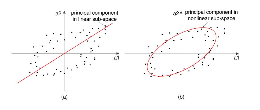
Instead of directly using the raw channel parameters ${\bf{a}}$, one possible approach could be to apply eigenvalue decomposition to decorrelate them, and then retain $M$ largest eigenvalues and corresponding eigenvectors, that can be used for ranging. This procedure is known as principal component analysis (PCA). However, PCA projects the data in a linear sub-space, so it is not useful if the data lies on a nonlinear manifold. An example for 2D data is shown in Fig. 1. Therefore, we propose to apply kernel PCA (kPCA) initially developed in its general form in [4]. kPCA differs from PCA in that it projects the data to an arbitrary nonlinear manifold. kPCA is already successfully applied to pattern recognition from images [4], and it is found that nonlinear principal components can provide much better recognition rates than corresponding linear principal components.

Figure 1: Principal components of 2D data in (a) linear and, (b) nonlinear sub-space. The latter one is much more accurate projection.

Consider a nonlinear transformation $\boldsymbol{\phi}({\bf{a}})$, which transforms $K$-dimensional vector ${\bf{a}}$ to an $N$-dimensional vector in a feature space. The feature space has large (possibly, infinite) dimension ($N>>K$). For now, we also assume that $\boldsymbol{\phi}({\bf{a}})$ has zero mean, so that its $N\times N$ covariance matrix is given by ${\bf{C}}=E(\boldsymbol{\phi}({\bf{a}})\boldsymbol{\phi}({\bf{a}})^{T})$. Then, we could find the principal components using eigenvalue expansion of ${\bf{C}}$, but this is not possible to compute explicitly since the feature space has high dimension. However, it can be shown [25, Chapter 12] that eigenvalue decomposition depends on $\boldsymbol{\phi}({\bf{a}})$ only via the inner product $k({\bf{a}},{\bf{a}}_{n})=\boldsymbol{\phi}({\bf{a}})^{T}\boldsymbol{\phi}({\bf{a}}_{n})$ (where ${\bf{a}}_{n}$ is a training sample, i.e., ${\bf{a}}_{n}\in\mathcal{T}$), known as a kernel function. Thus, we find principal components using the following eigenvalue expansion:

$${\bf{K}}{{\bf{v}}_{n}}={\lambda_{n}}N{{\bf{v}}_{n}}$$ (17)

where ${\bf{K}}$ is an $N\times N$ kernel matrix with $({{\bf{K}}})_{ij}=k({{\bf{a}}_{i}},{{\bf{a}}_{j}})$, $\forall{{\bf{a}}_{i}},{{\bf{a}}_{j}}\in\mathcal{T}.$ The eigenvalues and eigenvectors of ${\bf{K}}$ are given by $\lambda_{n}N$ and ${{\bf{v}}_{n}}$ ($n=1,\ldots,N$), respectively. Then, the projection of a test point ${\bf{a}}$ onto eigenvector $i$ is given by

$${y_{i}}({\bf{a}})=\sum\limits_{n=1}^{N}{{v_{in}}k({\bf{a}},{{\bf{a}}_{n}})}$$ (18)

Therefore, we can obtain all projections using kernel functions, without explicit work in feature space. In practice, the feature vector is not zero-mean, but it only means that we need to replace ${\bf{K}}$ with a Gram matrix ${\bf{\tilde{K}}}$:

$${\bf{\tilde{K}}}={\bf{K}}-{{\bf{1}}_{N}}{\bf{K}}-{\bf{K}}{{\bf{1}}_{N}}+{{\bf{1}}_{N}}{\bf{K}}{{\bf{1}}_{N}}$$ (19)

where ${{\bf{1}}_{N}}$ is the $N\times N$ matrix with all values equal to $1/N$. We see that this matrix can be also computed without the feature vectors. Therefore, for kPCA, we only need to define a kernel function. Popular choices [4] are Gaussian, sigmoid and polynomial kernels. Since we know that the range is a linear function of the TOA in case of LOS, and possibly a nonlinear function of all features in case of NLOS, a kernel that can model both linear and nonlinear relationships is appropriate. Therefore, we choose a polynomial kernel, given by:

$$k({\bf{a}},{{\bf{a}}_{n}})=({{\bf{a}}^{T}{{\bf{a}}_{n}}}+1)^{c}$$ (20)

where $c\in\mathbb{N}$ is the degree of the polynomial. The degree $c$ can be found empirically. Note that the standard PCA is a special case that results if we select the linear kernel $k({\bf{a}},{{\bf{a}}_{n}})={\bf{a}}^{T}{{\bf{a}}_{n}}$.

Then, given $M$ principal components ${y_{i}}({\bf{a}})$ corresponding to the $M$ largest eigenvalues, we need to provide a model that will relate them with the unknown range. Since this relationship is unknown in general, we use a simple linear model. A nonlinear model would be redundant anyway since we already had the opportunity to perform arbitrary nonlinear transformations using kPCA. Therefore, we assume that the projected features ${y_{i}}={y_{i}}({\bf{a}})$ are linear functions of the true distance:

$${y_{i}}={b_{1,i}}d+{b_{0,i}}+{\nu_{{y,i}}}$$ (21)

where ${b_{1,i}}$ and ${b_{0,i}}$ are parameters that can be found using least-squares curve fitting (using the same training samples, $\mathcal{T}$), and ${\nu_{{y,i}}}$ is a noise component. Since the distribution of the noise is also unknown, we assume that it is zero-mean Gaussian as the distribution that maximizes the entropy (given the variance $\sigma_{y,i}^{2}$, which can be found from the training samples). Assuming that we retain $M$ principal components, and taking into account that they are orthogonal to each other, the likelihood function is given by:

$$p({y_{1}},\ldots,{y_{M}}|d)=\prod\limits_{i=1}^{M}{p({y_{i}}|d)}=$$

$$~{}~{}~{}~{}~{}~{}~{}~{}\prod\limits_{i=1}^{M}{\mathcal{N}({y_{i}};{b_{1,i}}d+{b_{0,i}},\sigma_{y,i}^{2})}=$$

$$\prod\limits_{i=1}^{M}{\mathcal{N}\left({d;\frac{{{y_{i}}-{b_{0,i}}}}{{{b_{1,i}}}},\frac{{\sigma_{y,i}^{2}}}{{b_{1,i}^{2}}}}\right)}$$ (22)

The maximum number of principal components is equal to the total number of the training samples ($N$), which is much higher than the dimensionality of the original data ($K$). Since $M$ is expected to be larger than $K$, the main purpose of kPCA is nonlinear feature extraction, in contrast to PCA, which is typically used for dimensionality reduction.

From (IV-B), we can find the MMSE estimate of the distance,

$${\hat{d}_{kPCA}}=\sigma^{2}_{kPCA}\sum\limits_{i=1}^{M}{\left({{b_{1,i}}\frac{{{y_{i}}-{b_{0,i}}}}{{\sigma_{y,i}^{2}}}}\right)}$$ (23)

where

$$\sigma^{2}_{kPCA}={\left({\sum\limits_{i=1}^{M}{\frac{{b_{1,i}^{2}}}{{\sigma_{y,i}^{2}}}}}\right)^{-1}}$$ (24)

is the variance of the estimate. Recall that this estimate is valid for both LOS and NLOS scenarios, so NLOS identification is not needed. Assuming that eigenvalue decomposition is done offline, the complexity of kPCA is $\mathcal{O}(MN)$ since we need to find only $M$ principal components using (18). Therefore, kPCA is approximately $N/M$ times faster than GPR. However, this approach will provide a sub-optimal result since the noise in (21) is not Gaussian in the general case.

IV-C Hybrid methods: kPCA+ and kPCA+GPR

One problem of the kPCA and GPR methods described above is that they do not exploit the fact that some measurements will be LOS, and in that case the range can be directly obtained from the TOA. Hence, the kernel methods are only needed to handle NLOS measurements. However, since it may not be possible to make a reliable LOS/NLOS identification (i.e., estimate $H$), we need to use a soft-decision approach in a similar way as in Section III.

Since kPCA provides us many (up to $N$) projected features $y_{i}$, it is logical to assume that some of them will provide us useful information about $H$. However, the projected features represent a complex and unknown function of the raw channel parameters, so it is not easy to determine the precise model for the distribution $p(y_{i}|H)$. Therefore, using the same principle as in Section IV-B, we approximate this distribution with a Gaussian as follows:

$$p({y_{i}}|H)=\left\{\begin{array}[]{l}{\cal N}({y_{i}};{\mu_{L,{y_{i}}}},\sigma_{L,{y_{i}}}^{2}),\,\,\,\,\,{\rm{if}}\,\,\,H={\rm{LOS}}\\ {\cal N}({y_{i}};{\mu_{N,{y_{i}}}},\sigma_{N,{y_{i}}}^{2}),\,\,\,\,{\rm{if}}\,\,\,H={\rm{NLOS}}\end{array}\right.$$ (25)

where the parameters ${\mu_{L,{y_{i}}}}$, $\sigma_{L,{y_{i}}}$, ${\mu_{N,{y_{i}}}}$, $\sigma_{N,{y_{i}}}$ are found from the training set. This approximation will cause some loss of information, but we are now able to use multiple uncorrelated features, in contrast to the approach described in Section III. Consequently, the total likelihood function is given by:

$$p({y_{1}},\ldots,{y_{M^{\prime}}}|H)=\prod\limits_{i=1}^{M^{\prime}}{p({y_{i}}|H)}$$ (26)

where $M^{\prime}$ is the number of retained features for this classification problem (not necessarily equal to $M$). Then, the posterior distribution of $H$ is given by

$$p(H|{y_{1}},\ldots,{y_{M^{\prime}}})\propto p({y_{1}},\ldots,{y_{M^{\prime}}}|H)p(H)$$ (27)

where $p(H)$ is the prior distribution of $H$. Finally, the MMSE estimate of the distance is given by:

$$\hat{d}_{kPCA+}=p(H={\rm{LOS}}|{y_{1}},\ldots,{y_{M^{\prime}}})\left(c{\tau_{1}}-{\mu_{L}}\right)+$$

$$~{}~{}~{}~{}~{}~{}~{}p(H={\rm{NLOS}}|{y_{1}},\ldots,{y_{M^{\prime}}})\hat{d}_{kPCA}$$ (28)

where $\hat{d}_{kPCA}$ is the kPCA estimate of distance found by (23), but with one difference: the training set consists only of NLOS samples (the number of these samples is denoted by $N_{N}$). The variance of this estimate can be computed in the same fashion as the one in (III). Assuming that both eigenvalue decompositions are done offline, the complexity of this approach, referred to as kPCA+, is $\mathcal{O}(M^{\prime}N+MN_{N})$.

Alternatively, we may use GPR to estimate the distance from the NLOS training samples. In that case, the distance estimate is given by:

$$\hat{d}_{kPCA+GPR}=p(H={\rm{LOS}}|{y_{1}},\ldots,{y_{M^{\prime}}})\left(c{\tau_{1}}-{\mu_{L}}\right)+$$

$$~{}~{}~{}~{}~{}~{}~{}p(H={\rm{NLOS}}|{y_{1}},\ldots,{y_{M^{\prime}}})\hat{d}_{GPR}$$ (29)

The complexity of this approach, referred to as kPCA+GPR, is $\mathcal{O}(M^{\prime}N+N_{N}^{2})$. With a reasonable assumption that $N_{N}<<N$, kPCA+GPR would have a similar complexity as kPCA+, and would be much faster than original GPR.

A possible problem of the proposed kernel algorithms is the training phase, in which we need to collect enough measurements and corresponding ranges. This training can be done either offline or online, depending how variable the channel is in the considered environment. Since our goal is ranging using UWB signals (which can pass through thin obstacles [16]), the correct TOA can be estimated as long as the first path is detectable (even attenuated). Therefore, if the variability in the environment is caused by people walking or other thin objects (the required level of thinness depends on the signal bandwidth), the training can be done offline, as in the environment considered in the next section. Otherwise, e.g., in the presence of moving vehicles and other machinery, the training should be done online. In that case, a set of pre-deployed anchors on known (manually recorded) positions should be used. Their positions should be carefully chosen (e.g., uniformly deployed) in order to provide a sufficient statistics for training of parameters. This training can be repeated periodically (with a lower frequency than the online algorithm), or manually triggered once some change in the environment is detected. Since this procedure may be too slow in larger areas, the online training should be done only for the parts of the area in which the environmental changes are expected.

V Experimental Results

In this section, we analyze the performance of the proposed ranging methods using UWB measurements obtained in a basement tunnel of Linköping university (LiU) in Sweden.

V-A Measurement Setup and Scenarios

TABLE I: Measurement parameters

Parameter	Value
Signal power	12 dBm
Waveform	sinusoidal sweep
Center frequency	3.5 GHz
Bandwidth	2 GHz
Number of freq. points	3001
Sweep time	263 ms
Resolution	0.5 ns (15 cm)
Antenna range	1.71 - 6.4 GHz
Antenna gain	5 - 7.5 dBi
Cable attenuation	0.65 dB/m

Figure 2: Illustration of LOS experiments in LiU tunnel.

Figure 3: Deployment of transmitters (Tx) and receivers (Rx) in the LiU tunnel. There are 6 transmitter positions (marked with green squares), and 30 receiver positions (marked with red circles). Transmitters Tx 1-3 are used to test the LOS and two NLOS scenarios (by putting a metal sheet and a person in front of them), while transmitters Tx 4-6 are used to test NLOS caused by tunnel wall. The height of the tunnel is 2.8 m.

For our experiments, the measurement setup consisted of a vector network analyzer (VNA), two UWB omni-directional antennas and coaxial cables to connect the antennas with the VNA. A personal computer is used to set the VNA parameters and extract the multiple frequency responses from the VNA. We used a swept-frequency sinusoidal signal (with 3001 points) to characterize the channel between 2.5 and 4.5 GHz. The power level was set to 12 dBm, and a calibration of the system is performed to compensate for the effects of VNA, cables and antennas. Then, the frequency responses are transferred to the PC where a Hann window is used to reduce the out-of-band noise, and to ensure causality of the time-domain responses. Finally, by applying the Inverse Fast Fourier Transform (IFFT), the complex impulse responses are estimated, and then, PDPs are calculated. We summarize the main parameters in Table I.

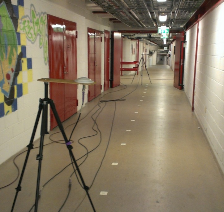
Using the described setup, the measurements have been carried out in a basement tunnel of LiU (Fig. 2). The tunnel walls, excluding the metal doors, are built of concrete blocks with steel reinforcement. The ceiling is also made of concrete, but with many metal pipes. Four different scenarios have been considered: LOS, and NLOS caused by three different obstacles: metal sheet, person, and tunnel wall. For each of these scenarios, we placed the transmitter (Tx) in 3 positions and receiver (Rx) in 30 positions forming the route through the tunnel, as shown in Fig. 3. For each Tx-Rx pair, we obtained 10 PDPs, so we obtained 3600 PDPs in total (900 per scenario). Since our initial analysis showed that thin obstacles (metal sheet and person) provide results similar as LOS (i.e., the direct path is detectable), we will consider them as LOS in the analyses. Therefore, we have available 2700 LOS samples and 900 NLOS samples. Half of these samples (1350 LOS samples and 450 NLOS samples) will be used as training data, and the rest will be used to test the ranging performance. Note that the training samples should include all the scenarios that are expected to be encountered in the online phase (i.e., LOS and all types of NLOS).

V-B Model Selection

TABLE II: The parameters estimated from the training samples.

Parameters	Estimated values
$\sigma_{L}$	0.16 m
$\sigma_{N}$	1.61 m
$\lambda_{L}$	0.333 ns-1
$\lambda_{N}$	0.075 ns-1
$(p_{2},p_{1},p_{0})$	$(0.00087,-0.2,11.72)$
$\boldsymbol{\theta}$	$(64.6,0.57,1.59)$
$\sigma_{\omega}$	0.5

We first extracted many parameters from the available PDPs (i.e., all parameters that have some physical meaning). Then, we tested the cross-correlation between each pair of parameters, and removed those that do not provide any additional information. From the remaining subset, we removed those which have negligible correlation with both the true range and the NLOS bias. The remaining $K=8$ channel parameters are used for kernel methods: TOA, RSS, maximum received power, mean excess delay, maximum excess delay, RMS delay spread, rise time and kurtosis (their definitions are available in [16, Section IV]). This parameter set is very similar to the sets [14, 10, 3, 17] widely used for ranging in indoor environments. For TOA with NLOS identification and error mitigation, we found that rise time is the best channel parameter ($\alpha_{I}$) for NLOS identification, and maximum excess delay is the best channel parameter ($\alpha_{E}$) for NLOS error mitigation. Regarding the model in (2), our measurements indicated that $\nu_{L}$ and $\nu_{N}$ approximately follow a zero-mean Gaussian distribution (with variances $\sigma_{L}^{2}$ and $\sigma_{N}^{2}$), while $g(\alpha_{E})$ can be modeled with a second-order polynomial function (i.e., $g({\alpha_{E}})=p_{2}{\alpha_{E}}^{2}+p_{1}{\alpha_{E}}+p_{0}$). The likelihood function $p({\alpha_{I}}|H)$ is assumed to follow an exponential distribution with different decay rates in the LOS and NLOS scenarios (given by $\lambda_{L}$ and $\lambda_{N}$, respectively), and the prior $p(H)$ is assumed to be non-informative. The justification of all these models is available in [16, Section V]. For the baseline GPR method, we used the Matlab toolbox (available online [26]) to obtain $\boldsymbol{\theta}$ and $\sigma_{\omega}$, and to perform the regression. The numerical values of all parameters are shown in Table II. We note the following: i) the standard deviation of the range estimate is much higher for the NLOS scenario ($\sigma_{N}>>\sigma_{L}$), ii) the LOS rise time decays much faster than the NLOS rise time ($\lambda_{L}>>\lambda_{N}$), and iii) the squared exponential term in the kernel, given by (11), has much higher influence than the linear term ($\theta_{0}>>\theta_{2}$). Note that these parameters are valid only for this specific environment, which means that the training phase should be repeated for the other environments.

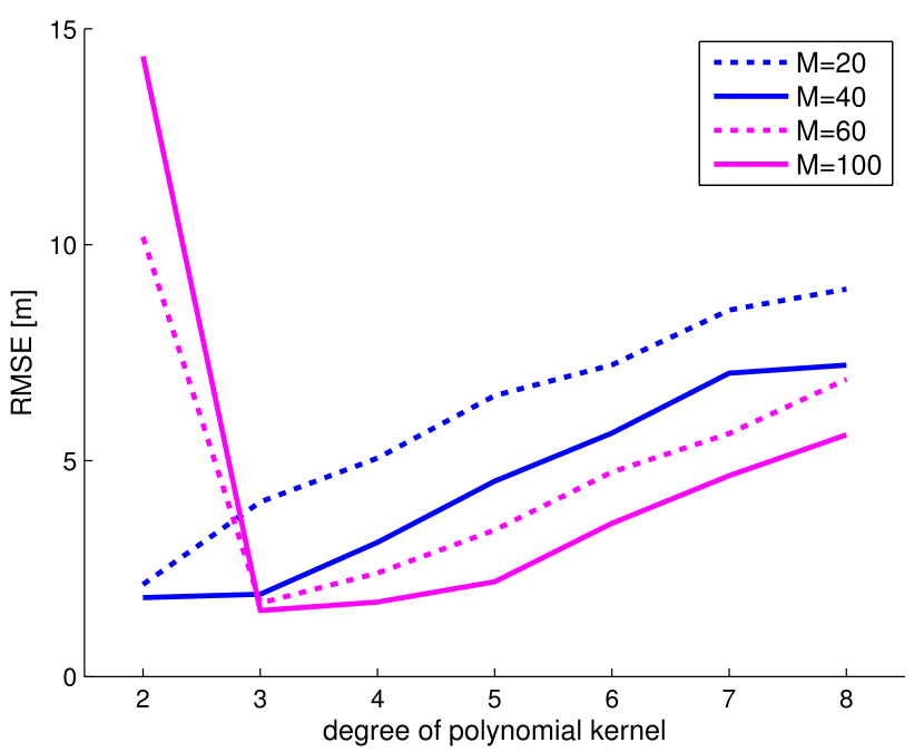
In order to empirically determine appropriate values of $c$ and $M$, we analyze root-mean-square error (RMSE) of the kPCA range estimates as a function of degree $c$, for different numbers of retained principal components $M$ (see Fig. 4). This metric is the most relevant for many applications, but note that in some cases other metrics (such as median, or 95% percentile) may be also useful. We see that it is necessary to retain $M\geq 40$ principal components. We choose $M=60$ principal components, in which case the best performance is achieved for $c=3$. We also note that a wrong value of the polynomial degree (e.g., $c=2$) could lead to a significant loss in performance. In general, too small values of $c$ would lead to under-fitting (i.e., the model is too simple), while too large values would lead to over-fitting (i.e, the model is too adapted to training samples).

Figure 4: RMSE as a function of degree of polynomial kernel ($c$) for different number of retained principal components ($M$).

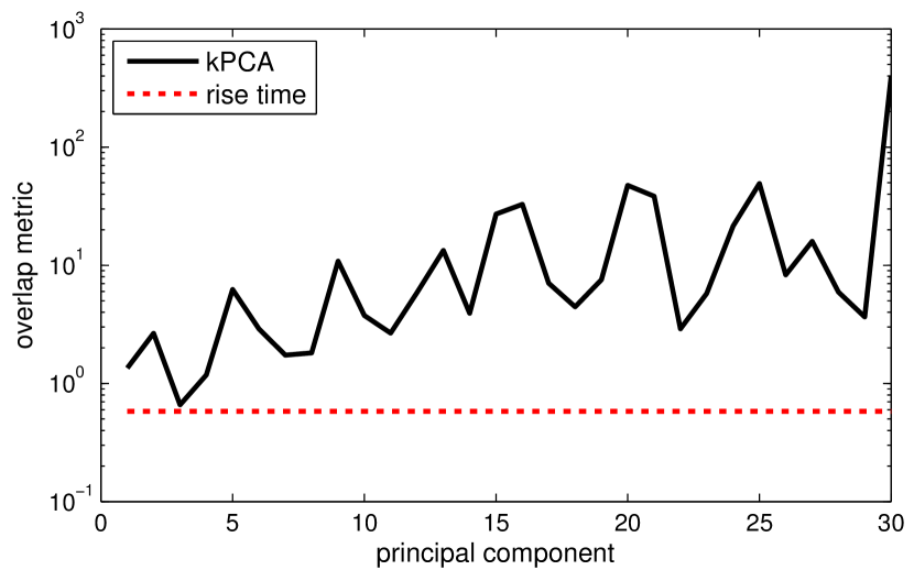
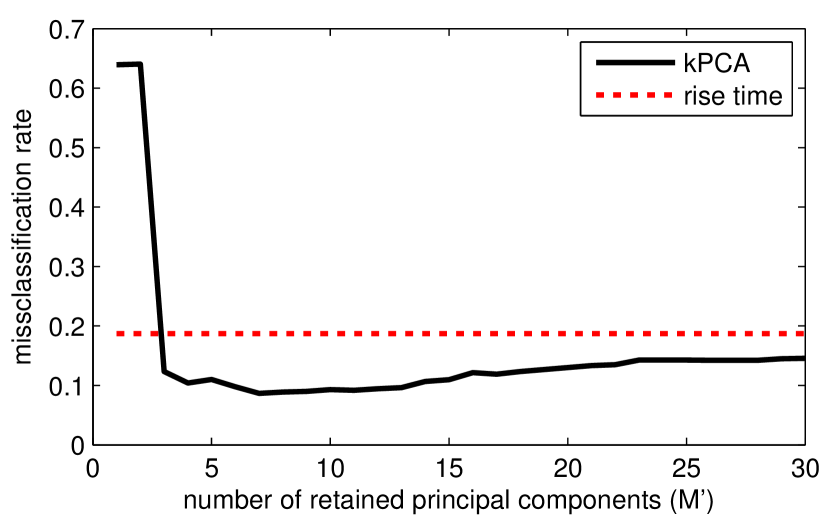
Regarding NLOS identification based on kPCA (needed for kPCA+ and kPCA+GPR), we analyze overlap metric [16], which represents a measure of the overlap of two distributions considering only their means and variances (defined as $\sqrt{\sigma_{L,{y_{i}}}\sigma_{N,{y_{i}}}}/\left|\mu_{L,{y_{i}}}-\mu_{N,{y_{i}}}\right|$ for $i$-th principal component), and misclassification rate (defined as $N_{miss}/N$, where $N_{miss}$ is the number of misclassifications). As we can see in Fig. 5a, the overlap between LOS and NLOS distributions have an oscillating behavior (as a function of $i$) and it is minimal for $i=3$. If we use only this principal component, we would not be able to perform better than the NLOS identification based on rise time. We also note an increasing tendency with $i$, since the higher principal components include little information (i.e., have small eigenvalues). Therefore, it is reasonable to use the first $M^{\prime}$ components as described in Section IV-C. In Fig. 5b, we can see that using kPCA for NLOS identification, instead of the approach based on rise time, can significantly reduce the misclassification rate with only $M^{\prime}\geq 3$ principal components (we choose $M^{\prime}=4$ for further analyses). On the other hand, the misclassification rate never reaches zero, which means that a soft-decision ranging algorithm is still required. The increasing tendency for $M^{\prime}>6$ is probably caused by the fact that the uncorrelated principal components are not necessarily independent.

(a)

(b)

Figure 5: NLOS identification using kPCA and rise time: (a) overlap metric for different principal components, and (b) misclassification rate as a function of $M^{\prime}$.

V-C Performance analysis

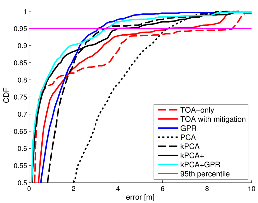
Given the previous models, our goal is to analyze the ranging error of the proposed algorithms and compare it with TOA-based methods and GPR. Therefore, we analyze the cumulative distribution function (CDF) of the ranging error, shown in Fig. 6. We observe the following:

• The TOA-only method provides very accurate results for about 77% of the samples (i.e., for all LOS and few NLOS samples). However, NLOS samples can cause a huge (up to 10 m) error. TOA with mitigation can reduce this error by about 1 m, but it performs slightly worse for LOS samples.

• The GPR method is the best approach for any percentile above the 90th, but it performs worse than TOA-based methods for the lower percentiles (i.e., mostly LOS samples). That can be explained by the fact that the GPR performs direct ranging using a combination of LOS and NLOS samples (without NLOS identification).

• The kPCA method performs slightly worse ($\sim 0.4$ m) than GPR for any percentile, due to the approximations made in (21). However, this method is about $N/M=30$ times faster than GPR. For the sake of completeness, we also show the performance of kPCA with the linear kernel (i.e., PCA), which provides a very poor performance, as expected.

• Both kPCA+ and kPCA+GPR methods, thanks to the NLOS identification, achieve the performance of the TOA-only method for LOS samples. For NLOS samples, they perform just slightly worse ($\sim$ 0.5-1 m) than GPR. Therefore, these two methods inherit the best characteristics of both state-of-the-art methods.

In summary, according to our experiments, kPCA+GPR (which is slightly more accurate than kPCA+), is more appropriate method for ranging than other considered state-of-the-art methods.

Figure 6: CDF of the ranging error for all considered algorithms. The results are based on 1800 test samples (of which $75\%$ are LOS and 25% are NLOS).

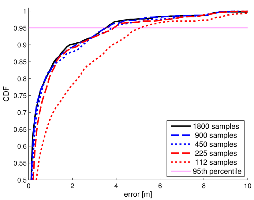
The previous analysis assumed that many training samples are available. We also analyze the effect of the number of training samples ($N$) on ranging accuracy, for two representative methods: GPR and kPCA+GPR. The results are shown in Fig. 7. As we can see, decreasing $N$ leads to reduced performance of GPR, so we need at least 450 samples to keep its performance reasonable. On the other hand, the performance of kPCA+GPR is nearly constant for $225\leq N\leq 1800$. The reason for somewhat remarkable behavior is twofold: i) classification is a discrete problem, in contrast to regression, ii) the kPCA+GPR estimates partly depend on TOA (see (IV-C)), which does not require any training samples. Therefore, an additional advantage of kPCA+GPR is that it requires fewer training samples, and consequently, it will be much faster. Moreover, we can observe that, for $100\leq N\leq 1500$ training samples, kPCA+GPR performs the best, while for $N>1500$, GPR provides the best performance. However, for very few training samples ($N<100$), both algorithms perform worse than TOA with mitigation (comparisons are done at 95th percentile). Consequently, a hybrid algorithm switching from one technique to another, depending on $N$, is also a reasonable option. In that case, the switching values depend on the environment, and can be found empirically.

(a)

(b)

Figure 7: CDF of the ranging error for different number of the training samples ($N$): (a) GPR, and (b) kPCA+GPR. The ratio between LOS and NLOS samples is preserved in all considered cases.

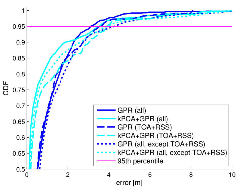
Finally, we analyze how different subsets of channel parameters affect the ranging performance. More specifically, we compare GPR and kPCA+GPR ranging methods based on i) all 8 channel parameters, ii) only TOA and RSS, and iii) all channel parameters except TOA and RSS. As we can observe in Fig. 8, it is beneficial to use more channel parameters for ranging. However, the gain is small (about 0.5 m) due to the partial correlations between these parameters (the correlation coefficients are available in [16, Table III]). Another important observation is that, if ranging is performed using all channel parameters except TOA and RSS, we can get a similar performance (for higher percentiles) as with ranging using TOA and RSS only. That means that ranging can be performed even without traditional metrics, such as TOA and RSS, which are used in many ranging and positioning algorithms. Therefore, kernel-based machine learning methods represent a very powerful toolbox since the same algorithm is able to adapt to different input measurements, even if they are related to the output in a complex nonlinear way.

We finish this section by summarizing the discussed characteristics of all considered methods in Table III.

Figure 8: CDF of the ranging error for different subsets of channel parameters.

TABLE III: A summary of the main characteristics of the considered ranging methods.

Ranging method	accuracy (50th/95th percentile)	complexity	required storage (excluding PDP)	NLOS identification	number of training samples
TOA-only	0.3 m / 9.1 m	$\mathcal{O}(1)$	$\mathcal{O}(1)$	no	0
TOA with mitigation	0.5 m / 6.3 m	$\mathcal{O}(1)$	$\mathcal{O}(1)$	yes	0
GPR	0.6 m / 3.1 m	$\mathcal{O}(N^{2})$	$\mathcal{O}(N^{2})$	no	large
kPCA	0.9 m / 3.5 m	$\mathcal{O}(MN)$	$\mathcal{O}(N^{2})$	no	large
kPCA+	0.2 m / 4.1 m	$\mathcal{O}(M^{\prime}N+MN_{N})$	$\mathcal{O}(N^{2}+N_{N}^{2})$	yes	small
kPCA+GPR	0.2 m / 3.5 m	$\mathcal{O}(M^{\prime}N+N_{N}^{2})$	$\mathcal{O}(N^{2}+N_{N}^{2})$	yes	small

VI Conclusions

We proposed novel kernel methods for UWB-based ranging, and tested them using real data from a tunnel environment. All methods are much faster than the state-of-the-art kernel method (GPR), since they use only a subset of orthogonal principal components. Among the proposed methods, the kPCA+GPR algorithm performs the best, and it outperforms both GPR and two TOA-based methods. In addition, compared to GPR, it requires fewer training samples. In summary, the moderate complexity and high ranging performance of kPCA+GPR makes this method useful for many critical applications, including emergency situations that require good performance within a short time.

There remain many interesting lines for possible future work. Since the kernel methods are trained to one particular, fixed environment, an extension to multiple different environments (e.g., by using online training) could be of high interest. It would also be useful to study whether GPR could be improved by replacing the Gaussian process with some other tractable random process. Finally, finding a tractable way to directly use channel impulse response measurements (i.e., without selection of features) may provide us even better ranging performance.

Vladimir Savic received the Dipl.Ing. degree in electrical engineering from the University of Belgrade, Belgrade, Serbia, in 2006, and the M.Sc. and Ph.D. degrees in communications technologies and systems from the Universidad Politecnica de Madrid, Madrid, Spain, in 2009 and 2012, respectively. He was a Digital IC Design Engineer with Elsys Eastern Europe, Belgrade, from 2006 to 2008. From 2008 to 2012, he was a Research Assistant with the Signal Processing Applications Group, Universidad Politecnica de Madrid, Spain. He spent three months as a Visiting Researcher at the Stony Brook University, NY, USA, and four months at the Chalmers University of Technology, Gothenburg, Sweden. In 2012, he joined the Communication Systems (CommSys) Division, Linköping University, Linköping, Sweden, as a Postdoctoral Researcher. He is co-author of more than 25 research papers in the areas of statistical signal processing and wireless communications. His research interests include localization and tracking, wireless channel modeling, Bayesian inference, machine learning and distributed and cooperative inference over wireless networks.

Erik G. Larsson received his Ph.D. degree from Uppsala University, Sweden, in 2002. Since 2007, he is Professor and Head of the Division for Communication Systems in the Department of Electrical Engineering (ISY) at Linköping University (LiU) in Linköping, Sweden. He has previously been Associate Professor (Docent) at the Royal Institute of Technology (KTH) in Stockholm, Sweden, and Assistant Professor at the University of Florida and the George Washington University, USA. In the spring of 2015, he was a Visiting Fellow at Princeton University, USA, for four months. His main professional interests are within the areas of wireless communications and signal processing. He has published some 100 journal papers on these topics, he is co-author of the textbook Space-Time Block Coding for Wireless Communications (Cambridge Univ. Press, 2003) and he holds 15 issued and many pending patents on wireless technology. He has served as Associate Editor for several major journals, including the IEEE Transactions on Communications (2010-2014) and IEEE Transactions on Signal Processing (2006-2010). He serves as chair of the IEEE Signal Processing Society SPCOM technical committee in 2015–2016 and as chair of the steering committee for the IEEE Wireless Communications Letters in 2014–2015. He is the General Chair of the Asilomar Conference on Signals, Systems and Computers in 2015 (he was Technical Chair in 2012). He received the IEEE Signal Processing Magazine Best Column Award twice, in 2012 and 2014, and he is receiving the IEEE ComSoc Stephen O. Rice Prize in Communications Theory in 2015.

Javier Ferrer-Coll received the B.Sc. degree in telecommunication engineering in 2005 and the M.Sc. in 2008 from the Universidad Politecnica de Valencia, Spain. He received his Ph.D in 2014, from the School of Information and Communication, Royal Institute of Technology (KTH), Stockholm, Sweden. From 2009 to 2014, he was employed at the university of Gävle, Sweden. He is currently employed as system engineer in the communication department at Combitech AB. His research interest is channel characterization in industrial environments, particularly measurement system design to extract the channel characteristics. Moreover, he is also interested in techniques to detect and suppress electromagnetic interferences.

Peter Stenumgaard has a Ph.D in radio communications from the Royal Institute of Technology (KTH), Stockholm. He is currently a Research Director and works as Head of the Department of Information Security & IT architecture at the Swedish Defence Research Agency (FOI) in Linköping, Sweden. He has worked as adjunct professor, both at Linköping University, Sweden, and the University of Gävle, Sweden. He has long experience of research for both military and civilian wireless applications and has also been the Director of the graduate school Forum Securitatis (funded by Vinnova) within Security and Crisis Management at Linköping University. He worked for several years on the JAS fighter aircraft project with the protection of aircraft systems against electromagnetic interference, lightning, nuclear weapon-generated electromagnetic pulse (EMP) and high-power microwaves (HPM). His research interests are robust telecommunications for military-, security-, safety- and industrial use.

References

- [1] V. Savic, E. G. Larsson, J. Ferrer-Coll, and P. Stenumgaard, “Kernel principal component analysis for UWB-based ranging,” in Proc. of IEEE Intl. Workshop on Signal Processing Advances in Wireless Communications (SPAWC), June 2014.
- [2] S. Gezici, Z. Tian, G. B. Giannakis, H. Kobayashi, A. F. Molisch, H. V. Poor, and Z. Sahinoglu, “Localization via ultra-wideband radios: a look at positioning aspects for future sensor networks,” IEEE Signal Processing Magazine, vol. 22, pp. 70–84, July 2005.
- [3] H. Wymeersch, S. Marano, W. M. Gifford, and M. Z. Win, “A machine learning approach to ranging error mitigation for UWB localization,” IEEE Trans. on Communications, vol. 60, pp. 1719 –1728, June 2012.
- [4] B. Scholkopf, A. J. Smola, and K.-R. Muller, Advances in kernel methods, ch. Kernel principal component analysis, pp. 327–352. Cambridge, MA, USA: MIT Press, 1999.
- [5] J. Khodjaev, Y. Park, and A. S. Malik, “Survey of NLOS identification and error mitigation problems in UWB-based positioning algorithms for dense environments,” Annals of telecommunications, vol. 65, no. 5-6, pp. 301–311, 2010.
- [6] M. P. Wylie and J. Holtzman, “The non-line of sight problem in mobile location estimation,” in Proc. of 5th IEEE Int. Universal Personal Communications Record. Conf, vol. 2, pp. 827–831, 1996.
- [7] J. Borris, P. Hatrack, and N. B. Manclayam, “Decision theoretic framework for NLOS identification,” in Proc. of IEEE Vehicular Technology Conf. (VTC), vol. 2, pp. 1583–1587, 1998.
- [8] S. Venkatesh and R. Buehrer, “Non-line-of-sight identification in ultra-wideband systems based on received signal statistics,” IET Microwaves, Antennas & Propagation, vol. 1, no. 6, pp. 1120–1130, 2007.
- [9] J. Zhang and E.-S. Lohan, “Analysis of kurtosis-based LOS/NLOS identification using indoor MIMO channel measurement,” IEEE Transactions on Vehicular Technology, vol. 62, pp. 2871–2874, July 2013.
- [10] S. Marano, W. Gifford, H. Wymeersch, and M. Win, “NLOS identification and mitigation for localization based on UWB experimental data,” IEEE Journal on Selected Areas in Communications, vol. 28, pp. 1026–1035, Sept. 2010.
- [11] S. Gezici, H. Kobayashi, and H. V. Poor, “Non-parametric non-line-of-sight identification,” in Proc. of IEEE Vehicular Technology Conf., vol. 4, (Orlando, FL), pp. 2544–2548, Oct. 2003.
- [12] S. Al-Jazzar, J. Caffery, and H.-R. You, “A scattering model based approach to NLOS mitigation in TOA location systems,” in Proc. of IEEE Vehicular Technology Conf. (VTC), vol. 2, pp. 861–865, 2002.
- [13] S. Al-Jazzar and J. Caffery, “ML and Bayesian TOA location estimators for NLOS environments,” in Proc. of IEEE Vehicular Technology Conf. (VTC), vol. 2, pp. 1178–1181, 2002.
- [14] B. Denis, J. Keignart, and N. Daniele, “Impact of NLOS propagation upon ranging precision in UWB systems,” in Proc. of IEEE Conf. on Ultra Wideband Systems and Technologies, pp. 379–383, 2003.
- [15] L. Cong and W. Zhuang, “Non-line-of-sight error mitigation in mobile location,” in Proc. of IEEE INFOCOM, p. 650 659, 2004.
- [16] V. Savic, J. Ferrer-Coll, P. Angskog, J. Chilo, P. Stenumgaard, and E. G. Larsson, “Measurement analysis and channel modeling for TOA-based ranging in tunnels,” IEEE Trans. on Wireless Communications, vol. 14, pp. 456–467, Jan. 2015.
- [17] T. V. Nguyen, Y. Jeong, H. Shin, and M. Z. Win, “Machine learning for wideband localization,” IEEE Journal on Selected Areas in Communications, vol. 33, pp. 1357–1380, July 2015.
- [18] N. Alsindi, X. Li, and K. Pahlavan, “Analysis of time of arrival estimation using wideband measurements of indoor radio propagations,” IEEE Transactions on Instrumentation and Measurement, vol. 56, pp. 1537–1545, Oct. 2007.
- [19] D. Dardari, A. Conti, U. Ferner, A. Giorgetti, and M. Z. Win, “Ranging with ultrawide bandwidth signals in multipath environments,” Proceedings of the IEEE, vol. 97, no. 2, pp. 404–426, 2009.
- [20] I. Guvenc and Z. Sahinoglu, “Threshold selection for UWB TOA estimation based on kurtosis analysis,” IEEE Communications Letters, vol. 9, pp. 1025–1027, Dec. 2005.
- [21] S. Venkatesh and R. Buehrer, “NLOS mitigation using linear programming in ultrawideband location-aware networks,” IEEE Transactions on Vehicular Technology, vol. 56, pp. 3182–3198, Sept. 2007.
- [22] I. Guvenc and C.-C. Chong, “A survey on TOA based wireless localization and NLOS mitigation techniques,” IEEE Communications Surveys & Tutorials, vol. 11, no. 3, pp. 107–124, 2009.
- [23] C. E. Rasmussen and C. K. I. Williams, Gaussian Processes for Machine Learning. MIT Press, 2006.
- [24] F. Perez-Cruz, S. V. Vaerenbergh, J. J. Murillo-Fuentes, M. Lazaro-Gredilla, and I. Santamaria, “Gaussian processes for nonlinear signal processing: An overview of recent advances,” IEEE Signal Processing Magazine, vol. 30, pp. 40–50, July 2013.
- [25] C. M. Bishop, Pattern Recognition and Machine Learning. Secaucus, NJ, USA: Springer-Verlag New York, Inc., 2006.
- [26] GPML Matlab Code. http://www.gaussianprocess.org/gpml/code/matlab/doc/.
![[Uncaptioned image]](/html/1511.04045/assets/VSavic.jpg) |