Progress in Electroweak Symmetry Breaking

Abstract:

In this talk, I discuss theoretical advances in understanding the properties of the Higgs boson and the implications for models of electroweak symmetry breaking. I begin by reviewing some of the recent progress in Standard Model calculations for Higgs boson production and decay rates, followed by a lightning tour of the use of effective field theories in the search for new physics in the Higgs sector. I end with a discussion of the complementarity of precision Higgs coupling measurements and direct searches for heavy particles for the discovery of Beyond the Standard Model physics in the electroweak sector.

1 Introduction

The experimental discovery of the Higgs boson marks a milestone in particle physics. With the confirmation that the Higgs boson is in general consistent with Standard Model (SM) expectations, the focus turns to precision measurements of Higgs properties and the implications for new physics[2]. The search for new physics in the electroweak sector depends crucially, however, on the comparison of precision calculations with measurements of Higgs properties. Although no deviations from Standard Model expectations have been observed in the Higgs- electroweak sector as of yet, unanswered questions about the pattern of fermions masses, the nature of dark matter, the source of CP violation, among many other questions, lead many physicists to expect Beyond the Standard Model (BSM) Physics at some as yet undetermined high mass scale. How this BSM physics might manifest itself at LHC energies is the source of considerable speculation and model building. BSM physics can lead to small deviations of Higgs couplings from their SM values. In addition, these models typically predict new Higgs-like bosons or heavy vector resonances. The search for these particles provides complementary information on BSM physics and is a major focus of Run-2 physics goals.

2 It Looks like the SM

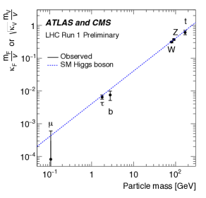
Figure 1: Relation between measured Higgs couplings and particle masses[2].

The SM is extremely predictive, with all Higgs properties except for the mass being determined. This characteristic makes it a testable (and falsifiable!) model. Run-1 of the LHC determined that the Higgs boson is charge -$0$, parity- even, and spin-$0$, with a mass $m_{h}=125.09\pm 0.21(stat)\pm 0.11(syst)GeV$[1]. Measurements of Higgs couplings are consistent with those predicted in the Standard Model at the $10-30\%$ level, and there is even some evidence that the Higgs couplings are proportional to fermion and gauge boson masses, as demonstrated in Fig. 1. All of these conclusions require theoretical calculations to the highest precision possible in the Standard Model. Only by direct comparison of the theory with experiment can we say that the observed particle is the SM Higgs boson.

3 Progress in Theory Calculations

3.1 Higher Order QCD Corrections

Higgs measurements are typically normalized relative to SM predictions. This makes it of utmost importance to have reliable theory predictions. The gold standard is becoming NNLO calculations, with many new results in the past year. The largest Higgs production rate is from gluon fusion and the cross section is known at 3-loops (NNNLO) in the $m_{t}\rightarrow\infty$ limit[3, 4]. The NNNLO corrections increase the rate by about $2\%$ from the NNLO prediction and reduce the scale uncertainty to $3-5\%$, as shown in 2. The most recent sets of PDFs[5] are in remarkable agreement in predicting the NNLO Higgs rate, and the PDF uncertainty on the gluon fusion production rate is now $\sim 2-3\%$[6], as seen in Fig. 3.

Searches for new physics often rely on observations in the high $p_{T}$ boosted regime, requiring precision calculations of Higgs plus jet distributions. Fully differential NNLO results including all initial parton states are now available[7, 8, 9] and are shown on the LHS of Fig. 4. The scale dependence is reduced from the NLO prediction, and the $K$ factor has a slight dependence on the transverse momentum of the Higgs boson. These calculations are also performed in the $m_{t}\rightarrow\infty$ limit.

The rate for vector boson fusion (VBF) of a Higgs boson is significantly smaller than that from gluon fusion, but VBF can provide a clean signal for precision measurements. VBF not only probes the Higgs couplings to gauge bosons, but eventually can be used to demonstrate that the Higgs boson unitarizes the $WW$ scattering cross sections[10]. An early calculation of VBF Higgs production at NNLO[11] found small effects from the QCD corrections, but a new fully differential calculation shows that when VBF kinematic cuts are imposed, the NNLO corrections can be of $\sim{\cal{O}}(10\%)$[12], as shown on the RHS of Fig. 4.

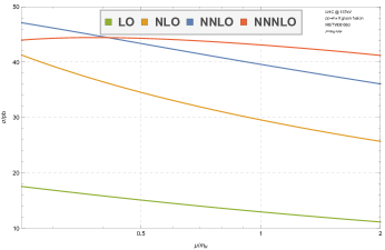
Figure 2: Scale dependence of the $gg\rightarrow h$ cross section at $\sqrt{S}=13~{}TeV$ at LO, NLO, NNLO, and NNNLO[3].

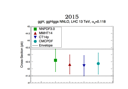
Figure 3: Dependence of NNLO Higgs cross section on the PDF choice at $\sqrt{S}=13~{}TeV$[6].

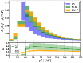
Figure 4: (a)$p_{T}$ dependence of the Higgs boson in $gg\rightarrow hjet$ at NNLO at $\sqrt{S}=13~{}TeV$[7]. (b) $p_{T}$ dependence of the Higgs boson in VBF at NNLO applying VBF cuts[12].

3.2 Measuring the Higgs Width

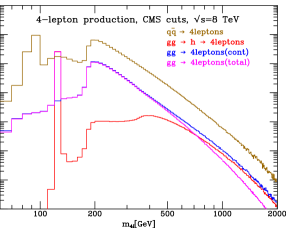
Figure 5: Contributions to $4$ lepton production at the LHC. The Higgs resonance contribution is the red line. [15]

In the SM, the Higgs total width is roughly $\Gamma_{h}^{SM}\sim 4~{}MeV$ and was long assumed to be unmeasurable since it is so much less than the LHC detectors’ resolutions. A few years ago, however, it was realized that by measuring $gg\rightarrow h\rightarrow ZZ\rightarrow 4l$ on the Higgs peak, $m_{4l}\sim m_{h}$, and comparing it with measurements of $m_{4l}$ above the resonance peak, one obtains a ratio that is sensitive to the Higgs width[13, 14, 15]. About $15\%$ of the cross section is in the region $m_{4l}>140~{}GeV$, as seen in Fig. 5, so this measurement appears feasible. The basic idea is that since the on-shell measurements of the Higgs cross section are consistent with SM expectations, a larger Higgs width would correspond to more off-shell events. Both CMS and ATLAS have used this idea to extract interesting limits on the Higgs width: $\Gamma_{h}^{ATLAS}<(4.5-7.5)\Gamma_{h}^{SM}$[16] (with the range corresponding to different assumptions about unknown radiative corrections) and $\Gamma_{h}^{CMS}<5.5\Gamma_{h}^{SM}$[17].

The problem with this approach is that it assumes that Higgs couplings are the same both on the Higgs resonance peak and above the peak. However, this is not the case if there is new physics (such as light colored particles) contributing to Higgs production, or if there are non-SM contributions to the decay due to anomalous Higgs couplings[18, 19]. As an example, consider a world where all couplings are SM- like except for the $tth$ and $ggh$ couplings,

$$L\sim-c_{t}{m_{t}\over v}{\overline{t}}th+{\alpha_{s}\over 12\pi}c_{g}{h\over v}G_{\mu\nu}^{a}G^{a.\mu\nu}\,.$$ (1)

(In the SM, $c_{t}=1$ and $c_{g}=0$). The gluon fusion production rate is sensitive to $\mid c_{t}+c_{g}\mid$, while the off- shell measurements of $gg\rightarrow ZZ\rightarrow 4l$ break this degeneracy. Fig. 6 shows the limits that can be extracted on $c_{g}$ and $c_{t}$ from the CMS $\sqrt{S}=8~{}TeV$ measurement of $gg\rightarrow ZZ\rightarrow 4l$. Imposing the restriction that $\mid c_{t}+c_{g}\mid=1$, one can extract the $68\%~{}$confidence level limit $-4<c_{t}<1.5$ or $2.9<c_{t}<6.1$[19]. The limit on $c_{t}$ will be improved by a direct measurement of $t{\overline{t}}h$ production in Run-2.

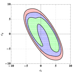
Figure 6: $68\%$, $95\%$, and $99\%$ confidence level limits on anomalous couplings from the off-shell measurement of $gg\rightarrow ZZ\rightarrow l^{+}l^{-}l^{+}l^{-}$ using the CMS 8 TeV data[19].

4 Fits to Higgs Couplings

4.1 The $\kappa$ approximation

One of the requirements for the observed scalar particle to be the Higgs boson of the SM is that its couplings be those predicted by the SM. The $\kappa$ formalism, used in analysing Run 1 Higgs data, simply rescales the Higgs couplings and total width from their SM values:

$$\kappa_{i}={g_{i}\over g_{SM}}\,,\qquad\kappa_{h}={\Gamma_{h}\over\Gamma_{h}^{SM}}\,.$$ (2)

This approach assumes that there are no new light particles, no new tensor structures in the Higgs interactions, that the narrow width approximation for Higgs decays is valid, and is based on rescaling total rates, ($\it{i.e.}$ no new dynamics is included). The fits are done under various assumptions about new physics in loops, ($\it{i.e.}$ the presence of new particles contributing to the $gg\rightarrow h$ or $h\rightarrow\gamma\gamma$ interactions) and about the possibility of a significant branching ratio of the Higgs to unobserved particles. No matter how the fits are performed, the conclusion is clear: Higgs couplings to gauge bosons and to third generation fermions must be within $10-30\%$ of their SM predictions[2].

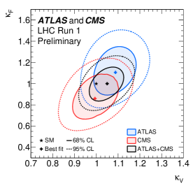
Figure 7: Combined CMS and ATLAS Higgs coupling fit when fermion and gauge boson couplings are rescaled in a universal manner[2].

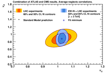
Figure 8: Gfitter global electroweak fit, combined with LHC Higgs data fit when Higgs fermion and gauge boson couplings are rescaled in an identical fashion[20].

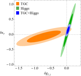
Figure 9: Limits from 3 gauge boson couplings (TGC) compared with limits from Higgs couplings on fits to dimension-6 EFT couplings[23].

A particularly simple fit can be done by assuming that all fermion and gauge boson couplings are rescaled in an identical fashion,

$$\kappa_{V} = \kappa_{W}=\kappa_{Z}$$

$$\kappa_{F} = \kappa_{t}=\kappa_{b}=\kappa_{\tau}=....$$ (3)

ATLAS and CMS have performed a combined fit[2], shown in Fig. 7, where the best fit value is remarkably close to the SM value of $\kappa_{V}=\kappa_{F}=1$. The impact of Higgs coupling measurements on global electroweak fits can be seen in the Gfitter[20] results of Fig. 8. The inclusion of the electroweak data significantly strengthens the bounds obtained from Higgs coupling fits alone. Similar results have been found in Ref. [21].

4.2 Higgs Effective Field Theory

The $\kappa$-formalism needs to be improved to analyse Run-2 data in order to incorporate kinematic information and electroweak radiative corrections into the fits. A consistent gauge invariant method to look for the effects of high mass BSM physics is the effective field theory technique (EFT) in which the SM is augmented by a series of higher dimension operators, ${\cal O}_{i}^{n}$,

$$L=L^{SM}+\Sigma_{n>4}\Sigma_{i}c_{i}^{n}{O_{i}^{n}\over\Lambda^{(n-4)}}\,.$$ (4)

The scale of new physics is generically taken to be $\Lambda$, and all operators allowed by the gauge symmetries must be included. In practice, only the dimension-$6$ operators, which are suppressed by factors of $1/\Lambda^{2}$, are likely to be numerically relevant. The coefficients of the EFT are constrained by global fits to Higgs couplings, along with precision electroweak measurements. In a specific BSM model, the coefficients are calculable and are in general related to each other. The importance of performing a global fit is demonstrated in Fig. 9 where the constraints from Higgs data are compared with those from the measurements of anomalous di-boson couplings[22, 23, 24]. The combination of Higgs data with that from 3 gauge boson vertices yields significantly stronger constraints than using either data set alone. Global fits using LHC-13 data to the suite of dimension-6 operators will provide significant constraints on BSM physics beyond the current limits.

The dimension-$6$ operators generate contributions which typically scale like ${p_{T}^{2}\over s}$ and so give enhanced effects in the large $p_{T}$ regime. These effects are shown in Fig. 10 for Higgs plus jet production, and for assumed values of $c_{t}$ and $\kappa_{g}\equiv c_{g}$ (${\it{cf}}$ Eq. 1). In the tail of the distribution, the effects of the non-SM couplings become visible. Note that $\mid c_{g}+\kappa_{g}\mid=1$ in this plot, so the single Higgs rate is unchanged. Fig. 11 demonstrates the effect of EFT couplings at high $p_{T}$ in $Zh$ production. Note that the contribution of the EFT operator is scaled up by a factor of $70$ in order to be visible. Including information from kinematic distributions, therefore, can potentially lead to significant improvements in the fits to EFT coefficients[24].

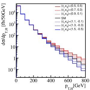
Figure 10: Higgs + jet production in the presence of anomalous couplings[25]. The couplings are chosen so as to leave the single Higgs production rate unchanged.

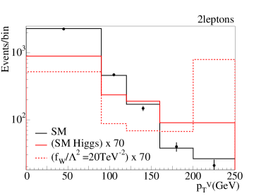
Figure 11: $p_{T}$ distribution for $Zh,Z\rightarrow l^{+}l^{-}$ production in the presence of the anomalous coupling $f_{W}$ at $\sqrt{S}=13~{}TeV$[24].

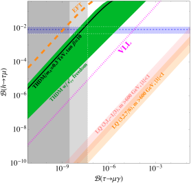
Figure 12: Correlation between $BR(\tau\rightarrow\mu\gamma)$ and $BR(h\rightarrow\tau\mu)$ in various BSM models (diagonal lines)[30]. The horizontal band is the CMS limit on $h\rightarrow\mu\tau$, when it is interpreted as a measurement[29].

5 Missing Information

Although the Higgs appears to be SM-like, we are missing a large amount of information. In particular, we know very little about the Yukawa couplings of the first and second generation fermions, about CP violating Higgs couplings, and about the flavor structure of the Higgs sector, to name just a few of our areas of ignorance.

5.1 2nd Generation Yukawa Couplings

At present there are no direct measurements of Higgs couplings to the second generation of fermions, although there are experimental limits on the coupling to muons which imply that $\kappa_{\mu}$ cannot be more than around $2$[2]. We also know very little about the charm quark Yukawa coupling. If $\kappa_{c}$ were extremely large, the production of $c{\overline{c}}\rightarrow h$ would dominate Higgs production. A direct measurement of the charm-Higgs coupling appears to be exceedingly difficult, leading to suggestions that the decay $h\rightarrow J/\Psi\gamma$ could potentially yield a measurement of $\kappa_{c}$, since $\Gamma(h\rightarrow J/\Psi\gamma)\sim\mid 12-\kappa_{c}\mid^{2}\times 10^{-10}~{}GeV$ has some sensitivity to $\kappa_{c}$. However, the small branching ratio, $BR(h\rightarrow J/\Psi\gamma)\sim(2.8-3.0)\times 10^{-6}$ implies that this measurement requires large luminosity[26, 27].

5.2 Flavor

Experimental limits on flavor in the Yukawa sector come from Higgs branching ratios, from searches for rare top decays, and low energy measurements. In the SM, the Higgs couplings are diagonal in flavor space, but it is straightforward to construct a model where this is not the case,

$$L\sim\lambda^{ij}{\overline{\Psi}}_{L}^{i}\Phi b_{R}^{j}+{\tilde{\lambda}}^{ij}{\overline{\Psi}}_{L}^{i}{\tilde{\Phi}}t_{R}^{j}+{c\over\Lambda^{2}}(\Phi^{\dagger}\Phi){\overline{\Psi}}_{L}^{i}\Phi b_{R}^{j}+{c^{\prime}\over\Lambda^{2}}(\Phi^{\dagger}\Phi){\overline{\Psi}}_{L}^{i}{\tilde{\Phi}}t_{R}^{j}+h.c.\,,$$ (5)

where $i,j$ are flavor indices, $\Psi_{L}^{i}$ are the fermion doublets and $\Phi$ is the Higgs doublet. In the absence of a dimension-$6$ contribution, $m_{b}^{ij}={\lambda^{ij}v\over\sqrt{2}}$, $m_{t}^{ij}={{\tilde{\lambda}}^{ij}v\over\sqrt{2}}$, and the mass matrices and Yukawa matrices are proportional to each other and simultaneously diagonalized. Once $c,c^{\prime}\neq 0$, these relationships are broken and the theory has flavor changing Higgs couplings, such as $t\rightarrow ch$, $h\rightarrow\mu e$, etc[28]. Flavor changing Higgs couplings in the lepton sector also contribute to low energy observables such as $\mu\rightarrow e\gamma$ and $\tau\rightarrow\mu\gamma$. There are complementary limits from processes such as $BR(h\rightarrow\tau\mu$) and $\tau\rightarrow\mu\gamma$ as shown in Fig. 12[30]. Interpreting the CMS limit on $h\rightarrow\mu\tau$[29] as a measurement gives the horizontal band in Fig. 12, while the diagonal lines are the predictions of some models with flavor violation in the Higgs sector. In general, there is a rich interplay between flavor violation in the Higgs sector and flavor violation in low energy observables.

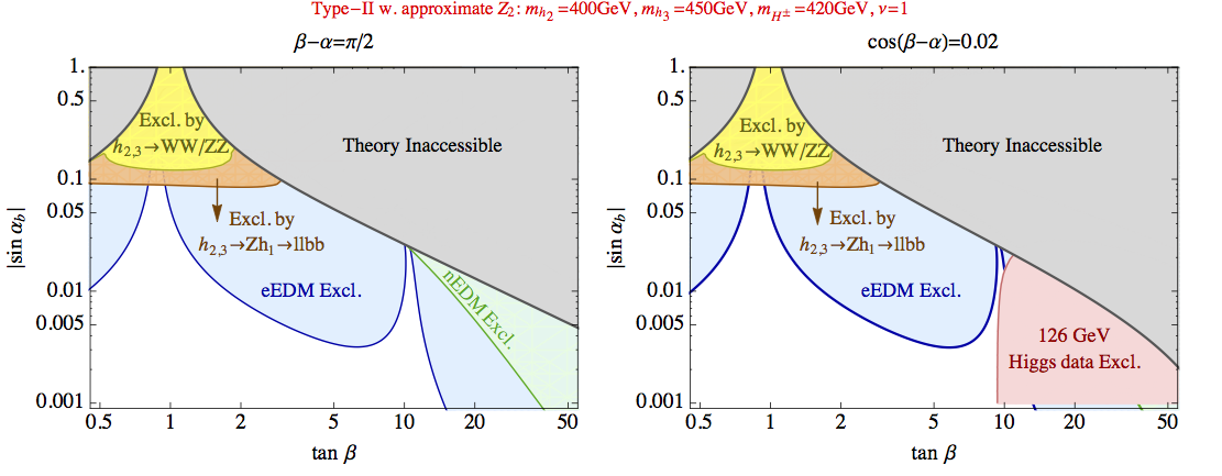
Figure 13: Limits on CP violation (parameterized by non-zero $sin~{}\alpha_{b}$) in the 2HDM [33].

5.3 CP Violation in the Higgs Sector

In the SM, all Higgs couplings are real and there is no CP violation. The simplest way to introduce CP violation is in the context of the 2HDM, where complex Higgs couplings are possible, leading to mixing between the $2$ neutral scalars and the pseudoscalar boson . These couplings change the rates for Higgs decays, and also change the predictions for electron and neutron EDMs[31, 32, 33]. A summary of current bounds is in Fig. 13, where the CP violation is parameterized by non-zero $\sin\alpha_{b}$. It is clear that the direct search for heavy Higgs bosons, the measurement of Higgs couplings, and limits from electron and neutron EDMs all probe complementary regions of parameter space.

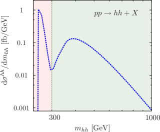
Figure 14: Higgs singlet model prediction for $gg\rightarrow hh$ at $\sqrt{S}=14~{}TeV$ with $M_{H}=255~{}GeV$ and parameters adjusted such that $\sigma/\sigma_{SM}=2.8$[35].

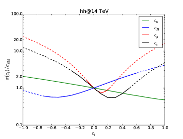
Figure 15: Sensitivity of the $gg\rightarrow hh$ cross section to anomalous couplings. The coefficients defined in Eq. 5.2 are normalized such that $c_{i}=0$ corresponds to the SM. The dotted lines are incompatible with single Higgs measurements[40].

5.4 Exploring the Higgs Potential

In the minimal SM, the Higgs tri-linear coupling, $\lambda_{3}={m_{h}^{2}\over 2v^{2}}\sim.13$, is a firm prediction of the model, and the measurement of $\lambda_{3}$ is a vital test of the structure of the SM potential. This coupling is probed by the process $gg\rightarrow hh$, which has an extremely small rate in the SM: $\sigma_{NNLO}\sim 34.3~{}fb$ at $\sqrt{S}=13~{}TeV$[34], where the NNLO rate is known in the $m_{t}\rightarrow\infty$ approximation. The small rate makes double Higgs production quite sensitive to new physics effects, in particular in scenarios where a resonant enhancement from a $2^{nd}$ neutral Higgs particle, $H$, is possible. In cases where $M_{H}\sim 250-500~{}GeV$, enhancements of the rate by factors of up to $20$ are possible[35, 36, 37, 38, 39], along with distortions of the kinematic distributions, as illustrated in Fig. 14. The dip in the distribution is due to interference effects between the contributions of the $2$ neutral scalars.

Double Higgs production can also be enhanced by factors of $2-3$ due to anomalous couplings [40, 41, 42, 43], and the $t{\overline{t}}hh$ coupling, which is typical of composite Higgs models [44], is particularly interesting. Dimension-$6$ couplings affecting double Higgs production can be parameterized as

$$L\sim{c_{H}\over 2v^{2}}(\partial^{\mu}\mid\Phi\mid^{2})^{2}-{c_{6}\over v^{2}}\lambda_{3}\mid\Phi\mid^{6}+{\alpha_{s}\over 4\pi}{c_{g}\over v^{2}}\mid\Phi\mid^{2}G_{\mu\nu}^{a}G^{a,\mu\nu}-\biggl{(}{c_{t}\over v^{2}}{\sqrt{2}m_{t}\over v}\mid\Phi\mid^{2}{\overline{\Psi_{L}}}{\tilde{\Phi}}t_{R}+h.c.\biggr{)}\,,$$ (6)

and the effects of varying one coefficient at a time are shown in Fig. 15.

6 Naturalness and the Search for New Physics

Despite the impressive agreement of Higgs measurements with predictions, the theory is unsatisfactory. In the EFT language, BSM physics generically gives contributions to the Higgs mass of ${\cal{O}}(M_{h}^{2}\sim\Lambda^{2})$. This has led to proposals for models where a symmetry prohibits large contributions to the Higgs mass from the high scale physics–the MSSM and NMSSM are examples of this class of model. The Higgs sector of the 2HDM illustrates many of the features of the more complicated models[45]. In the 2HDM, the new physics is probed by the search for the heavier Higgs state and also by precision Higgs couplings. The Higgs couplings depend on the usual $\tan\beta$ and a mixing parameter, $\cos(\alpha-\beta)$, and there are four possible assignments of fermion couplings which do not lead to tree level flavor changing neutral currents. Direct searches for the heavier Higgs boson are complementary to precision Higgs coupling measurements and both are needed to probe the parameter space. This is illustrated in Fig. 16[46, 47] for two different fermion-Higgs coupling assignments.

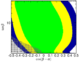
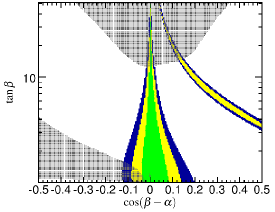
Figure 16: Complementarity of limits from direct searches for the heavy Higgs boson of a CP conserving 2HDM with $M_{H}=300~{}GeV$ (gray shaded) with limits from the precision measurements of the $125~{}GeV$ Higgs couplings[46]. LHS: Type-I 2HDM and RHS: Type-II 2HDM. SM couplings are obtained in the limit $\cos(\alpha-\beta)=1$.

An alternative possibility for solving the problem of large contributions to the Higgs mass from BSM high scale physics is the composite Higgs scenario, where the observed Higgs particle is a pseudo Nambu Goldstone boson[44]. These models contain heavy vector resonances which are limited by direct search results. Again, complimentary limits are found from precision measurements of Higgs couplings and from the direct searches, as seen in Fig.17.

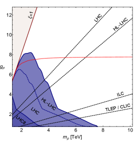
Figure 17: Complementarity of direct searches for a heavy vector resonance of a composite Higgs model compared with limits extracted from Higgs coupling measurements. The dotted lines are projected limits from Higgs coupling measurements at the LHC ($\sqrt{S}=14~{}TeV$ with $300~{}fb^{-1}$) and ILC ($\sqrt{S}=500~{}GeV$ with $500~{}fb^{-1}$). Above the red line $\Gamma_{\rho}/m_{\rho}>20\%$.[48]

7 Outlook

The past year has seen immense progress in the study of electroweak symmetry breaking. Combined ATLAS/CMS measurements of Higgs properties, along with NNLO calculations allow for precision tests of the SM paradigm and test BSM physics at the $TeV$ scale. These limits are often complementary to those obtained from low energy observables. Run-2 will probe even higher scales of new physics both by direct searches for new particles and by precise measurements of EFT couplings. It is possible that new physics lies just around the corner!

References

- [1] G. Aad et al. [ATLAS and CMS Collaborations], Phys. Rev. Lett. 114, 191803 (2015) [arXiv:1503.07589 [hep-ex]].
- [2] The ATLAS and CMS Collaborations, ATLAS-CONF-2015-044.
- [3] C. Anastasiou, C. Duhr, F. Dulat, F. Herzog and B. Mistlberger, Phys. Rev. Lett. 114, 212001 (2015) [arXiv:1503.06056 [hep-ph]].
- [4] C. Anastasiou, C. Duhr, F. Dulat, E. Furlan, F. Herzog and B. Mistlberger, JHEP 1508, 051 (2015) [arXiv:1505.04110 [hep-ph]].
- [5] J. Rojo et al., J. Phys. G 42, 103103 (2015) [arXiv:1507.00556 [hep-ph]].
- [6] S. Forte, Contribution to Higgs Hunting 2015 Conference.
- [7] R. Boughezal, C. Focke, W. Giele, X. Liu and F. Petriello, Phys. Lett. B 748, 5 (2015) [arXiv:1505.03893 [hep-ph]].
- [8] R. Boughezal, F. Caola, K. Melnikov, F. Petriello and M. Schulze, Phys. Rev. Lett. 115, no. 8, 082003 (2015) [arXiv:1504.07922 [hep-ph]].
- [9] F. Caola, K. Melnikov and M. Schulze, arXiv:1508.02684 [hep-ph].
- [10] B. W. Lee, C. Quigg and H. B. Thacker, Phys. Rev. D 16, 1519 (1977).
- [11] P. Bolzoni, F. Maltoni, S. O. Moch and M. Zaro, Phys. Rev. Lett. 105, 011801 (2010) [arXiv:1003.4451 [hep-ph]].
- [12] M. Cacciari, F. A. Dreyer, A. Karlberg, G. P. Salam and G. Zanderighi, Phys. Rev. Lett. 115, no. 8, 082002 (2015) [arXiv:1506.02660 [hep-ph]].
- [13] F. Caola and K. Melnikov, Phys. Rev. D 88, 054024 (2013) [arXiv:1307.4935 [hep-ph]].
- [14] N. Kauer and G. Passarino, JHEP 1208, 116 (2012) [arXiv:1206.4803 [hep-ph]].
- [15] J. M. Campbell, R. K. Ellis and C. Williams, JHEP 1404 (2014) 060 [arXiv:1311.3589 [hep-ph]].
- [16] G. Aad et al. [ATLAS Collaboration], Eur. Phys. J. C 75, no. 7, 335 (2015) [arXiv:1503.01060 [hep-ex]].
- [17] V. Khachatryan et al. [CMS Collaboration], Phys. Lett. B 736, 64 (2014) [arXiv:1405.3455 [hep-ex]].
- [18] C. Englert, Y. Soreq and M. Spannowsky, JHEP 1505, 145 (2015) [arXiv:1410.5440 [hep-ph]].
- [19] A. Azatov, C. Grojean, A. Paul and E. Salvioni, Zh. Eksp. Teor. Fiz. 147, 410 (2015) [J. Exp. Theor. Phys. 120, 354 (2015)] [arXiv:1406.6338 [hep-ph]].
- [20] M. Baak et al. [Gfitter Group Collaboration], Eur. Phys. J. C 74, 3046 (2014) [arXiv:1407.3792 [hep-ph]].
- [21] J. de Blas, M. Ciuchini, E. Franco, D. Ghosh, S. Mishima, M. Pierini, L. Reina and L. Silvestrini, arXiv:1410.4204 [hep-ph].
- [22] T. Corbett, O. J. P. boli, J. Gonzalez-Fraile and M. C. Gonzalez-Garcia, Phys. Rev. Lett. 111, 011801 (2013) [arXiv:1304.1151 [hep-ph]].
- [23] A. Falkowski, M. Gonzalez-Alonso, A. Greljo and D. Marzocca, arXiv:1508.00581 [hep-ph].
- [24] T. Corbett, O. J. P. Eboli, D. Goncalves, J. Gonzalez-Fraile, T. Plehn and M. Rauch, JHEP 1508, 156 (2015) [arXiv:1505.05516 [hep-ph]].
- [25] M. Schlaffer, M. Spannowsky, M. Takeuchi, A. Weiler and C. Wymant, Eur. Phys. J. C 74, no. 10, 3120 (2014) [arXiv:1405.4295 [hep-ph]].
- [26] G. T. Bodwin, F. Petriello, S. Stoynev and M. Velasco, Phys. Rev. D 88, no. 5, 053003 (2013) [arXiv:1306.5770 [hep-ph]].
- [27] M. K nig and M. Neubert, JHEP 1508, 012 (2015) [arXiv:1505.03870 [hep-ph]].
- [28] R. Harnik, J. Kopp and J. Zupan, JHEP 1303, 026 (2013) [arXiv:1209.1397 [hep-ph]].
- [29] CMS Collaboration, CMS-PAS-HIG-14-040, 2015.
- [30] I. Dor ner, S. Fajfer, A. Greljo, J. F. Kamenik, N. Ko nik and I. Ni and ic, JHEP 1506, 108 (2015) [arXiv:1502.07784 [hep-ph]].
- [31] G. C. Branco, P. M. Ferreira, L. Lavoura, M. N. Rebelo, M. Sher and J. P. Silva, Phys. Rept. 516, 1 (2012) [arXiv:1106.0034 [hep-ph]].
- [32] D. Fontes, J. C. Rom o, R. Santos and J. P. Silva, Phys. Rev. D 92, no. 5, 055014 (2015) [arXiv:1506.06755 [hep-ph]].
- [33] C. Y. Chen, S. Dawson and Y. Zhang, JHEP 1506, 056 (2015) [arXiv:1503.01114 [hep-ph]].
- [34] D. de Florian and J. Mazzitelli, JHEP 1509, 053 (2015)
- [35] M. J. Dolan, C. Englert and M. Spannowsky, Phys. Rev. D 87, no. 5, 055002 (2013) [arXiv:1210.8166 [hep-ph]].
- [36] T. Robens and T. Stefaniak, Eur. Phys. J. C 75, 104 (2015) [arXiv:1501.02234 [hep-ph]].
- [37] C. Y. Chen, S. Dawson and I. M. Lewis, Phys. Rev. D 91, no. 3, 035015 (2015) [arXiv:1410.5488 [hep-ph]].
- [38] J. Baglio, O. Eberhardt, U. Nierste and M. Wiebusch, Phys. Rev. D 90, no. 1, 015008 (2014) [arXiv:1403.1264 [hep-ph]].
- [39] B. Hespel, D. Lopez-Val and E. Vryonidou, JHEP 1409, 124 (2014) [arXiv:1407.0281 [hep-ph]].
- [40] F. Goertz, A. Papaefstathiou, L. L. Yang and J. Zurita, JHEP 1504, 167 (2015) [arXiv:1410.3471 [hep-ph]].
- [41] M. Gillioz, R. Grober, C. Grojean, M. Muhlleitner and E. Salvioni, JHEP 1210, 004 (2012) [arXiv:1206.7120 [hep-ph]].
- [42] A. Azatov, R. Contino, G. Panico and M. Son, Phys. Rev. D 92, no. 3, 035001 (2015) [arXiv:1502.00539 [hep-ph]].
- [43] C. Y. Chen, S. Dawson and I. M. Lewis, Phys. Rev. D 90, no. 3, 035016 (2014) [arXiv:1406.3349 [hep-ph]].
- [44] G. Panico and A. Wulzer, arXiv:1506.01961 [hep-ph].
- [45] H. E. Haber and D. O’Neil, Phys. Rev. D 83, 055017 (2011) [arXiv:1011.6188 [hep-ph]].
- [46] H. E. Haber and O. St l, Eur. Phys. J. C 75, no. 10, 491 (2015) [arXiv:1507.04281 [hep-ph]].
- [47] C. Y. Chen, S. Dawson and M. Sher, Phys. Rev. D 88, 015018 (2013) [Phys. Rev. D 88, 039901 (2013)] [arXiv:1305.1624 [hep-ph]].
- [48] A. Thamm, R. Torre and A. Wulzer, JHEP 1507, 100 (2015) [arXiv:1502.01701 [hep-ph]].