Separable Potentials for (d,p) Reaction Calculations

Abstract

An important ingredient for applications of nuclear physics to e.g. astrophysics or nuclear energy are the cross sections for reactions of neutrons with rare isotopes. Since direct measurements are often not possible, indirect methods like $(d,p)$ reactions must be used instead. Those $(d,p)$ reactions may be viewed as effective three-body reactions and described with Faddeev techniques. An additional challenge posed by $(d,p)$ reactions involving heavier nuclei is the treatment of the Coulomb force. To avoid numerical complications in dealing with the screening of the Coulomb force, recently a new approach using the Coulomb distorted basis in momentum space was suggested. In order to implement this suggestion, one needs to derive a separable representation of neutron- and proton-nucleus optical potentials and compute their matrix elements in this basis.

1 Introduction

Nuclear reactions are an important probe to learn about the structure of unstable nuclei. Due to the short lifetimes involved, direct measurements are usually not possible. Therefore indirect measurements using ($d,p$) reactions have been proposed (see e.g. Refs. [1, 2, 3]). Deuteron induced reactions are particularly attractive from an experimental perspective, since deuterated targets are readily available. From a theoretical perspective they are equally attractive because the scattering problem can be reduced to an effective three-body problem [4]. Traditionally deuteron-induced single-neutron transfer ($d,p$) reactions have been used to study the shell structure in stable nuclei, nowadays experimental techniques are available to apply the same approaches to exotic beams (see e.g. [5]). Deuteron induced $(d,p)$ or $(d,n)$ reactions in inverse kinematics are also useful to extract neutron or proton capture rates on unstable nuclei of astrophysical relevance. Given the many ongoing experimental programs worldwide using these reactions, a reliable reaction theory for $(d,p)$ reactions is critical.

One of the most challenging aspects of solving the three-body problem for nuclear reactions is the repulsive Coulomb interaction. While the Coulomb interaction for light nuclei is often a small correction to the problem, this is certainly not the case for intermediate mass and heavy systems. Over the last decade, many theoretical efforts have focused on advancing the theory for $(d,p)$ reactions (e.g. [6, 7]) and testing existing methods (e.g. [8, 4, 9]). Currently, the most complete implementation of the theory is provided by the Lisbon group [10], which solves the Faddeev equations in the Alt, Grassberger and Sandhas [11] formulation. The method introduced in [10] treats the Coulomb interaction with a screening and renormalization procedure as detailed in [12, 13]. While the current implementation of the Faddeev-AGS equations with screening is computationally effective for light systems, as the charge of the nucleus increases technical difficulties arise in the screening procedure [14]. Indeed, for most of the new exotic nuclei to be produced at the Facility of Rare Isotope Beams, the current method is not adequate. Thus one has to explore solutions to the nuclear reaction three-body problem where the Coulomb problem is treated without screening.

In Ref. [6], a three-body theory for $(d,p)$ reactions is derived with explicit inclusion of target excitations, where no screening of the Coulomb force is introduced. Therein, the Faddeev-AGS equations are cast in a Coulomb-distorted partial-wave representation, instead of a plane-wave basis. This approach assumes the interactions in the two-body subsystems to be separable. While in Ref. [6] the lowest angular momentum in this basis ($l=0$) is derived for a Yamaguchi-type nuclear interaction is derived as analytic expression, it is desirable to implement more general form factors, which are modeled after the nuclei under consideration.

In order to bring the three-body theory laid out in Ref. [6] to fruition, well defined preparatory work needs to be successfully carried out. Any momentum space Faddeev-AGS type calculation needs as input transition matrix elements in the different two-body subsystems. In the case of ($d,p$) reactions with nuclei these are the $t$-matrix elements obtained from the neutron-proton, the neutron-nucleus and proton-nucleus interactions. Since it is essential to use separable interactions when solving the Faddeev equations in the Coulomb basis, those need to be developed not only in the traditionally employed plane wave basis, but also the basis of Coulomb scattering states.

In this contribution major developments needed to provide reliable input to a Faddeev-AGS formulation of $(d,p)$ reactions in the Coulomb basis are summarized. Those are the derivation of separable representations of neutron-nucleus and proton-nucleus optical potentials. Here it is important that those representations not only describe the cross sections for elastic scattering accurately, but also allow to represent a wide variety of nuclei. Furthermore, it should be straightforward to generalize the representation to account for excitations of the nuclei.

2 Separable Representation of Nucleon-Nucleus Optical Potentials

Separable representations of the forces between constituents forming the subsystems in a Faddeev approach have a long tradition in few-body physics. There is a large body of work on separable representations of nucleon-nucleon (NN) interactions (see e.g. Refs. [15, 16, 17, 18, 19]) or meson-nucleon interactions [20, 21]. In the context of describing light nuclei like ⁶He [22] and ⁶Li [23] in a three-body approach, separable interactions have been successfully used. A separable nucleon-¹²C optical potential was proposed in Ref. [24], consisting of a rank-1 Yamaguchi-type form factor fitted to the positive energies and a similar term describing the bound states in the nucleon-¹²C configuration. However, systematic work along this line for heavy nuclei, for which excellent phenomenological descriptions exist in terms of Woods-Saxon functions [25, 26, 27, 28] has not been carried out until recently [29].

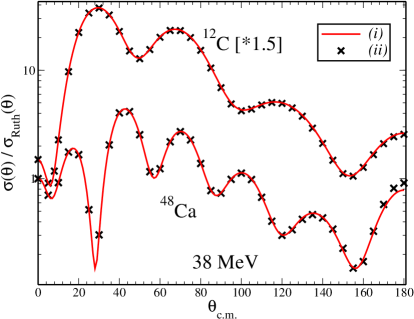
Figure 1: The unpolarized differential cross section for elastic scattering of protons from ¹²C (upper) and ⁴⁸Ca (lower) divided by the Rutherford cross section as function of the c.m. angle calculated for E_lab = 38 MeV. The ¹²C cross section is scaled by a factor 1.5. The solid lines ($i$) depict the cross section calculated in momentum space based on the rank-4 separable representation of the CH89 [25] phenomenological optical potential, while the cross symbols ($ii$) represent the corresponding coordinate space calculations.

The separable representation of two-body interactions suggested by Ernst-Shakin-Thaler [30] (EST) is well suited for achieving this goal. We note that this EST approach has been successfully employed to represent NN potentials [15, 16]. However, the EST scheme derived in Ref. [30], though allowing energy dependence of the potentials [31, 32], assumes that they are Hermitian. Therefore, we generalized the EST approach in Ref. [29] in order to be applicable for optical potentials which are complex. Here it is important that the reaction matrix elements constructed from these separable potentials satisfy reciprocity relations.

In analogy to the procedure followed in Ref. [30] we define a complex separable potential of arbitrary rank in a given partial wave as

$${\bf U}=\sum_{i,j}u|f_{l,k_{E_{i}}}\rangle\langle f_{l,k_{E_{i}}}|M|f^{*}{{}_{l},k_{E_{j}}}\rangle\langle f^{*}_{l,k_{E_{j}}}|u.$$ (1)

Here $f_{l,k_{E}}(r)$ is the unique regular radial wave function corresponding to $u$ and $f^{*}_{l,k_{E}}(r)$ is the unique regular radial wavefunction corresponding to $u^{*}$, where $u$ is the potential for which the separable representation is constructed. The EST scheme guarantees that at the fixed set of energies ${E_{i}}$ (support points) the wave functions obtained with the original potential $u$ and those obtained with the separable representation $U$ are identical. The matrix $M$ is defined and constrained by

$$\delta_{ik}=\sum_{j}\langle f_{l,k_{E_{i}}}|M|f^{*}_{l,k_{E_{j}}}\rangle\langle f^{*}_{l,k_{E_{j}}}|u|f_{l,k_{E_{k}}}\rangle=\sum_{j}\langle f^{*}_{l,k_{E_{i}}}|u|f_{l,k_{E_{j}}}\rangle\langle f_{l,k_{E_{j}}}|M|f^{*}_{l,k_{E_{k}}}\rangle.$$ (2)

The corresponding separable partial wave $t$-matrix must be of the form

$$t(E)=\sum_{i,j}u|f_{l,k_{E_{i}}}\rangle\tau_{ij}(E)\langle f^{*}_{l,k_{E_{j}}}|u\;,$$ (3)

with the following restrictions

$$\delta_{nj} = \sum_{i}\langle f^{*}_{l,k_{E_{n}}}|u-ug_{0}(E)u|f_{l,k_{E_{i}}}\rangle\;\tau_{ij}(E),$$ (4)

$$\delta_{ik} = \sum_{j}\tau_{ij}(E)\;\langle f^{*}_{l,k_{E_{j}}}|u-ug_{0}(E)u|f_{l,k_{E_{k}}}\rangle,$$ (5)

which are used to obtain the matrix $\tau_{ij}(E)$. In general, optical potentials are energy dependent. Though the wave functions $f_{l,k_{E_{i}}}$ carry part of this energy dependence, the EST scheme needs to be extended to exactly take into account energy dependent potentials [32, 33].

Extending the EST separable representation to the Coulomb basis involves replacing the neutron-nucleus half-shell $t$-matrix in Eq. (3) by Coulomb distorted scattering states $|f^{c}_{l,p}\rangle$, which defines the Coulomb-distorted separable nuclear $t$-matrix

$$\tau^{CN}_{l}(E)=\sum_{i,j}u_{l}^{s}|f^{c}_{l,k_{E_{i}}}\rangle\;\tau^{c}_{ij}(E)\;\langle f^{c\;,\;*}_{l,\;k_{E_{j}}}|u_{l}^{s}.$$ (6)

Here $|f^{c}_{l,k_{E_{i}}}\rangle$ and $|f^{c\;,\;*}_{l,k_{E_{i}}}\rangle$ are the regular radial Coulomb scattering wave functions, corresponding to $u_{l}^{s}$ and $(u_{l}^{s})^{*}$ at energy $E_{i}$. The constraints are similar to those of Eqs. (4) and (5). The Coulomb Green’s function is given as $g_{c}(E+i\varepsilon)=(E+i\varepsilon-H_{0}-v^{C})^{-1}$ with $H_{0}$ being the free Hamiltonian and $v^{C}$ the point Coulomb potential. It remains to calculate the half-shell $t$-matrix at the support points in the Coulomb basis. Here we follow the method suggested in  [34] and successfully applied in [35], and note that in this case the Coulomb Green’s function behaves like a free Green’s function.

For studying the quality of the representation of proton-nucleus optical potentials we consider p+¹²C and p+⁴⁸Ca elastic scattering and show the unpolarized differential cross sections divided by the Rutherford cross section as function of the c.m. angle $\theta_{c.m.}$ in Fig. 1. First, we observe very good agreement in both cases of the momentum space calculations using the separable representation with the corresponding coordinate space calculations. Second, we want to point out that we used for the separable representation of the proton-nucleus partial-wave $t$-matrices the same support points as in the neutron-nucleus case. This makes the determination of suitable support points $E_{i}$ for a given optical potential and nucleus quite efficient.

3 Separable Representation of Multi-Channel Optical Potentials

For representing the NN interaction with a separable interaction, the EST scheme had to be extended to include channel coupling [15, 16] e.g. in the deuteron channel. For describing $(d,p)$ reactions within a Faddeev-AGS approach, this is a natural channel coupling to include. However, for $(d,p)$ on nuclei, specifically exotic nuclei, which are often deformed, one also has to consider possible excitations of those nuclei. In the formulation of Ref. [6] the three-body theory to include excitations is layed out. Again, we need to construct separable representations for optical potentials that include excitations of the nucleus, e.g. rotational degrees of freedom.

To extend the EST scheme to non-Hermitian coupled channel potentials, we define for a fixed total angular momentum $J$

$$U^{J} = \sum\limits_{\rho\sigma}\sum\limits_{mn}\left(\sum\limits_{\nu}u\Big{|}\Psi_{\nu\rho,k_{m}^{\rho}}^{(+)J}\mathcal{Y}_{\nu}^{JM}\Big{\rangle}\right)\lambda_{mn}^{\rho\sigma}\left(\sum\limits_{\nu}\Big{\langle}\Psi_{\nu\sigma,k_{n}^{\sigma}}^{(-)J}\mathcal{Y}_{\nu}^{JM}\Big{|}u\right)$$ (7)

$$\equiv \sum\limits_{\rho\sigma}\sum\limits_{mn}T(E_{m})\Big{|}\mathcal{Y}_{\rho}^{JM}\phi_{l_{\rho}k_{m}}\Big{\rangle}\lambda_{mn}^{\rho\sigma}\Big{\langle}\phi_{l_{\sigma}k_{n}^{\sigma}}\mathcal{Y}_{\sigma}^{JM}\Big{|}T(E_{n}),$$ (8)

where $\langle\Psi_{\nu\sigma,k_{n}^{\sigma}}^{(+)J}|$ are the solutions of the coupled-channel Lippmann-Schwinger equation corresponding to $u$ and $\langle\Psi_{\nu\sigma,k_{n}^{\sigma}}^{(-)J}$) those corresponding to $u^{\dagger}$ with incoming boundary conditions. The indices $\rho$ and $\sigma$ indicate the coupling between channels, while $m$ and $n$ refer to the rank of the separable representation. The constraints necessary to satisfy the EST conditions become

$$\delta_{mi}\delta_{\rho\gamma} = \sum\limits_{\sigma n}\sum\limits_{\nu}\lambda_{mn}^{\rho\sigma}\Big{\langle}\phi_{l_{\sigma}k_{n}^{\sigma}}\mathcal{Y}_{\sigma}^{JM}\Big{|}T(E_{n})\Big{|}\mathcal{Y}_{\gamma}^{JM}\Psi_{\nu\gamma,k_{i}^{\gamma}}^{(+)J}\Big{\rangle},$$ (9)

$$= \sum\limits_{\sigma n}\sum\limits_{\nu}\Big{\langle}\Psi_{\nu\gamma,k_{i}^{\gamma}}^{(-)J}\mathcal{Y}_{\nu}^{JM}\Big{|}T(E_{n})\Big{|}\mathcal{Y}_{\sigma}^{JM}\phi_{l_{\sigma}k_{n}^{\sigma}}\Big{\rangle}\lambda_{nm}^{\sigma\rho}.$$ (10)

The multi-channel separable $t$-matrix then takes the form

$$t_{\alpha\beta}^{J}(k^{\prime},k;E) = \sum\limits_{\rho\sigma}\sum\limits_{mn}T^{J}_{\alpha\rho}(k^{\prime},k_{m}^{\rho};E_{m})\tau_{mn}^{\rho\sigma}(E){T}^{J}_{\sigma\beta}(k,k_{n}^{\sigma};E_{n}),$$ (11)

$$= \sum\limits_{ab}T^{J}_{\alpha a}(k^{\prime},k_{a};E_{a})\tau_{ab}(E){T}^{J}_{b\beta}(k,k_{b};E_{b}),$$ (12)

where the quantities $T^{J}_{\alpha\rho}(k^{\prime},k_{a};E_{a})$ represent the half-shell transition matrix elements in channels $\alpha$ and $\rho$. The coupling matrix $\tau_{mn}^{\rho\sigma}(E)$ depends now on the rank, indicated by the indices $m$ and $n$ as well as on the channels indicated by the superscripts. Simplyfing the quadrupel sum of the first row in Eq. (12) over rank as well as channel indices to a double sum over leads to the second row. Explicitly, the coupling matrix $\tau(E)$ is calculated as

$$[\tau(E)]_{ab}^{-1} = \Big{\langle}\phi_{l_{a}k_{a}}\mathcal{Y}_{\alpha_{a}}^{JM}\Big{|}T(E_{a})\Big{|}\mathcal{Y}_{\alpha_{b}}^{JM}\phi_{l_{b}k_{b}}\Big{\rangle}$$ (13)

$$+ \sum\limits_{\beta}\int\limits_{0}^{\infty}dp\;p^{2}\;\Big{\langle}\phi_{l_{a}k_{a}}\mathcal{Y}_{\alpha_{a}}^{JM}\Big{|}T(E_{a})\Big{|}\mathcal{Y}_{\beta}^{JM}\phi_{l_{\beta}p}\Big{\rangle}G_{\beta}(E_{b})\Big{\langle}\phi_{l_{\beta}p}\mathcal{Y}_{\alpha_{a}}^{JM}|T(E_{b})\Big{|}\mathcal{Y}_{\alpha_{b}}^{JM}\phi_{l_{b}k_{b}}\Big{\rangle}$$

$$- \sum\limits_{\beta}\int\limits_{0}^{\infty}p^{2}dp\;\Big{\langle}\phi_{l_{a}k_{a}}\mathcal{Y}_{\alpha_{a}}^{JM}\Big{|}T(E_{a})\Big{|}\mathcal{Y}_{\beta}^{JM}\phi_{l_{\beta}p}\rangle G_{\beta}(E)\Big{\langle}\phi_{l_{\beta}p}\mathcal{Y}_{\beta}^{JM}|T(E_{b})\Big{|}\mathcal{Y}_{\alpha_{b}}^{JM}\phi_{l_{b}k_{b}}\Big{\rangle}.$$

Here $G_{\beta}(E)=(E-\varepsilon_{\beta}-E_{p}^{\beta}+i\epsilon)^{-1}$ is the channel Green’s function with $E_{p}^{\beta}=p^{2}/2\mu_{\beta}$, with $\mu_{\beta}$ being the reduced mass in the channel $\beta$.

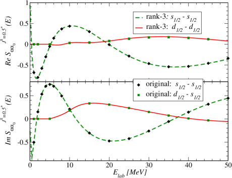
Figure 2: The separable representation of rank 3 for the s-d multichannel S-matrix $S_{\alpha\alpha_{0}}^{J}(E)$ for $n$+¹²C scattering as function of the laboratory kinetic energy for $J^{\pi}=\frac{1}{2}^{+}$. The $0^{+}\otimes s_{1/2}-0^{+}\otimes s_{1/2}$ and $2^{+}\otimes d_{1/2}-0^{+}\otimes s_{1/2}$ $S$-matrix elements are indicated by the (green) dashed and (red) solid lines. The EST support points are given at 6, 20, and 40 MeV. The $S$-matrix elements obtained using the original potential are shown for comparison.

As example for constructing a separable optical potential including rotational excitations we use the potential from Ref. [36] which describes elastic and inelastic scattering of neutrons from ¹²C in the energy range 16.5 to 22 MeV. This potential includes the excitation $I^{\pi}=2^{+}$ and $I^{\pi}=4^{+}$ at 4.44 MeV and 14.08 MeV in ¹²C, and takes into account quadrupole and octupole deformations. In Fig. 2 we focus on the on-shell properties of the potential up to 50 MeV laboratory kinetic energy. The EST support points are chosen to be at 6, 20, and 45 MeV. In Fig. 2 the multi-channel $S$-matrix elements are depicted for calculations based on the original potential and on its separable representation. The calculations indicate that the extension of the EST formulation which includes excitations of the nucleus represents the original optical potential very well, and thus those potentials can serve as input for $(d,p)$ reaction calculations.

4 Summary and Outlook

In a series of steps we developed the input that will serve as a basis for Faddeev-AGS three-body calculations of $(d,p)$ reactions, which will not rely on the screening of the Coulomb force. To achieve this, Ref. [6] formulated the Faddeev-AGS equations in the Coulomb basis using separable interactions in the two-body subsystems. For this ambitious program to have a chance of being successful, the interactions in the two-body subsystems, namely the NN and the neutron- and proton-nucleus systems, need to developed so that they separately describe the observables of the subsystems. While for the NN interaction separable representations are available, this is was not the case for the optical potentials describing the nucleon-nucleus interactions. Furthermore, those interactions in the subsystems need to be available in the Coulomb basis.

We developed separable representations of phenomenological optical potentials of Woods-Saxon type for neutrons and protons. First we concentrated on neutron-nucleus optical potentials and generalized the Ernst-Shakin-Thaler (EST) scheme [30] so that it can be applied to complex potentials [29]. In order to consider proton-nucleus optical potentials, we further extended the EST scheme so that it can be applied to the scattering of charged particles with a repulsive Coulomb force [37]. While the extension of the EST scheme to charged particles led to a separable proton-nucleus $t$-matrix in the Coulomb basis, we had to develop methods to reliably compute Coulomb distorted neutron-nucleus $t$-matrix elements [38]. Here we also show explicitly that those calculations can be carried out numerically very accurately by calculating them within two independent schemes. We also showed that the scheme can be further extended to take channel coupling into account.

Our results demonstrate, that our separable representations reproduce standard coordinate space calculations of neutron and proton scattering cross sections very well, and that we are able to accurately compute the integrals leading to the Coulomb distorted form factors. Now that these challenging form factors have been obtained, they can be introduced into the Faddeev-AGS equations to solve the three-body problem without resorting to screening. Our expectation is that solutions to the Faddeev-AGS equations written in the Coulomb-distorted basis can be obtained for a large variety of $n+p+A$ systems, without a limitation on the charge of the target. From those solutions, observables for $(d,p)$ transfer reactions should be readily calculated. Work along these lines is in progress.

References

References

- [1] Escher J E, Burke J T, Dietrich F S, Scielzo N D, Thompson I J and Younes W 2012 Rev. Mod. Phys. 84(1) 353–397 URL http://link.aps.org/doi/10.1103/RevModPhys.84.353
- [2] Cizewski J et al. 2013 J. Phys. Conf 420 012058
- [3] Kozub R, Arbanas G, Adekola A, Bardayan D, Blackmon J et al. 2012 Phys.Rev.Lett. 109 172501
- [4] Nunes F and Deltuva A 2011 Phys.Rev. C84 034607
- [5] Schmitt K, Jones K, Bey A, Ahn S, Bardayan D et al. 2012 Phys.Rev.Lett. 108 192701
- [6] Mukhamedzhanov A, Eremenko V and Sattarov A 2012 Phys.Rev. C86 034001
- [7] Deltuva A 2013 Phys.Rev. C88 011601 (Preprint 1307.0997)
- [8] Deltuva A, Moro A, Cravo E, Nunes F and Fonseca A 2007 Phys.Rev. C76 064602 (Preprint 0710.5933)
- [9] Upadhyay N, Deltuva A and Nunes F 2012 Phys.Rev. C85 054621 (Preprint 1112.5338)
- [10] Deltuva A and Fonseca A 2009 Phys.Rev. C79 014606
- [11] Alt E, Grassberger P and Sandhas W 1967 Nucl. Phys. B 2 167
- [12] Deltuva A, Fonseca A and Sauer P 2005 Phys.Rev. C71 054005
- [13] Deltuva A, Fonseca A and Sauer P 2005 Phys.Rev. C72 054004
- [14] Nunes F and Upadhyay N 2012 J. Phys. G: Conf. Ser. 403 012029
- [15] Haidenbauer J and Plessas W 1983 Phys.Rev. C27 63–70
- [16] Haidenbauer J, Koike Y and Plessas W 1986 Phys.Rev. C33 439–446
- [17] Berthold G, Stadler A and Zankel H 1990 Phys.Rev. C41 1365–1383
- [18] Schnizer W and Plessas W 1990 Phys.Rev. C41 1095–1099
- [19] Entem D, Fernandez F and Valcarce A 2001 J.Phys. G27 1537–1546
- [20] Ueda T and Ikegami Y 1994 Prog.Theor.Phys. 91 85–104
- [21] Gal A and Garcilazo H 2011 Nucl.Phys. A864 153–166
- [22] Ghovanlou A and Lehman D R 1974 Phys. Rev. C9 1730–1741
- [23] Eskandarian A and Afnan I R 1992 Phys. Rev. C46 2344–2353
- [24] Miyagawa K and Koike Y 1989 Prog. Theor. Phys. 82 329
- [25] Varner R, Thompson W, McAbee T, Ludwig E and Clegg T 1991 Phys.Rept. 201 57–119
- [26] Weppner S, Penney R, Diffendale G and Vittorini G 2009 Phys.Rev. C80 034608
- [27] Koning A and Delaroche J 2003 Nucl.Phys. A713 231–310
- [28] Becchetti FD J and Greenlees G 1969 Phys.Rev. 182 1190–1209
- [29] Hlophe L et al. (The TORUS Collaboration) 2013 Phys.Rev. C88 064608 (Preprint 1310.8334)
- [30] Ernst D J, Shakin C M and Thaler R M 1973 Phys.Rev. C8 46–52
- [31] Ernst D, Londergan J, Moniz E and Thaler R 1974 Phys.Rev. C10 1708–1721
- [32] Pearce B 1987 Phys.Rev. C36 471–474
- [33] Hlophe L and Elster C in preparation.
- [34] Elster C, Liu L C and Thaler R M 1993 J.Phys. G19 2123–2134
- [35] Chinn C R, Elster C and Thaler R M 1991 Phys.Rev. C44 1569–1580
- [36] Olsson B, Trostell B and Ramstrom E 1989 Nucl.Phys.A 469 505
- [37] Hlophe L, Eremenko V, Elster C, Nunes F M, Arbanas G, Escher J E and Thompson I J 2014 Phys. Rev. C90 061602 (Preprint 1409.4012)
- [38] Upadhyay N et al. (TORUS Collaboration) 2014 Phys. Rev. C90 014615