Steady solutions of the
Navier-Stokes equations
in the plane

Abstract

This study is devoted to the incompressible and stationary Navier-Stokes equations in two-dimensional unbounded domains. First, the main results on the construction of the weak solutions and on their asymptotic behavior are reviewed and structured so that all the cases can be treated in one concise way. Most of the open problems are linked with the case of a vanishing velocity field at infinity and this will be the main subject of the remainder of this study. The linearization of the Navier-Stokes around the zero solution leads to the Stokes equations which are ill-posed in two dimensions. It is the well-known Stokes paradox which states that if the net force is nonzero, the solution of the Stokes equations will grow at infinity. By studying the link between the Stokes and Navier-Stokes equations, it is proven that even if the net force vanishes, the velocity and pressure fields of the Navier-Stokes equations cannot be asymptotic to those of the Stokes equations. However, the velocity field can be in some cases asymptotic to two exact solutions of the Stokes equations which also solve the Navier-Stokes equations. Finally, a formal asymptotic expansion at infinity for the solutions of the two-dimensional Navier-Stokes equations having a nonzero net force is established based physical arguments. The leading term of the velocity field in this expansion decays like $\left|\boldsymbol{x}\right|^{-1/3}$ and exhibits a wake behavior. Numerical simulations are performed to validate this asymptotic expansion when is net force is nonzero and to analyze the asymptotic behavior in the case where the net force is vanishing. This indicates that the Navier-Stokes equations admit solutions whose velocity field goes to zero at infinity in contrast to the Stokes linearization and moreover this shows that the set of possible asymptotes is very rich.

Keywords: Navier-Stokes equations, Stokes equations, Steady solutions, Numerical simulations

MSC class: 35Q30, 35J57, 76D05, 76D07, 76D03, 76D25, 76M10

Chapter 1 Introduction

We consider a viscous fluid of constant viscosity $\mu$ and constant density $\rho$ moving in a region $\Omega$ of the two or three-dimensional space. The motion of the fluid is characterized by the velocity field $\boldsymbol{u}(\boldsymbol{x},t)$ and the pressure field $p(\boldsymbol{x},t)$, where $\boldsymbol{x}\in\Omega$ is the position and $t>0$ the time. In an inertial frame, the equations of motion are given by

$$\rho\left(\frac{\partial\boldsymbol{u}}{\partial t}+\boldsymbol{u}\boldsymbol{\cdot}\boldsymbol{\nabla}\boldsymbol{u}\right) =\mu\Delta\boldsymbol{u}-\boldsymbol{\nabla}p-\rho\boldsymbol{f}\,, \boldsymbol{\nabla}\boldsymbol{\cdot}\boldsymbol{u} =\boldsymbol{0}\,,$$ (1)

where $\boldsymbol{f}$ is minus the external force per unit mass acting on the fluid. These equations were first described by Navier (1827, p. 414), but their adequate physical justification was given only later on in the work of Stokes (1845). Nowadays, these equations are referred to as the Navier-Stokes equations. The resolution of the Navier-Stokes equations consists of finding fields $\boldsymbol{u}$ and $p$ satisfying (LABEL:intro-ns-time) together with some prescribed boundary conditions or initial conditions. The beginning of mathematical fluid dynamics started with the pioneering work of Leray (1933) who developed a general method for solving the Navier-Stokes equations essentially without any restriction on the size of the data. With the usage of computers, the Navier-Stokes equations can now be solved numerically with good precision in many cases, which is crucial for applications. However, up to this date, the Navier-Stokes equations are far from being completely understood mathematically. One major question is the one stated by the Clay Mathematical Institute as one of the seven most important open mathematical problems: do the time-dependent Navier-Stokes equations in an unbounded or periodic domain of the three-dimensional space admit a solution for large data? Ladyzhenskaya (1969) answers the same question affirmatively in two dimensions. A second major question concerns the steady solutions in two-dimensional unbounded domains, which is the main subject of this research. For time-independent domains, steady motions are described by $\partial_{t}\boldsymbol{u}=\partial_{t}\boldsymbol{f}=\boldsymbol{0}$, which leads to the following stationary Navier-Stokes equations,

$$\mu\Delta\boldsymbol{u}-\boldsymbol{\nabla}p =\rho\left(\boldsymbol{u}\boldsymbol{\cdot}\boldsymbol{\nabla}\boldsymbol{u}+\boldsymbol{f}\right)\,, \boldsymbol{\nabla}\boldsymbol{\cdot}\boldsymbol{u} =\boldsymbol{0}\,.$$ (2)

Various aspects of these equations have been studied: the monograph of Galdi (2011) presents them in great detail. By the change of variables

$$\boldsymbol{u} \mapsto\frac{\mu}{\rho}\boldsymbol{u}\,, p\mapsto \frac{\mu^{2}}{\rho}p\,, \boldsymbol{f} \mapsto\frac{\mu^{2}}{\rho^{2}}\boldsymbol{f}\,,$$

the parameters $\mu$ and $\rho$ can be set to one,

$$\Delta\boldsymbol{u}-\boldsymbol{\nabla}p =\boldsymbol{u}\boldsymbol{\cdot}\boldsymbol{\nabla}\boldsymbol{u}+\boldsymbol{f}\,, \boldsymbol{\nabla}\boldsymbol{\cdot}\boldsymbol{u} =0\,,$$ (3a)

as we will do from now on. In case the domain $$\Omega \partial\Omega$$ has a boundary , we complete (LABEL:intro-ns-eq) with a condition that describes how the fluid interacts with the boundary,

$$\left.\boldsymbol{u}\right|_{\partial\Omega}=\boldsymbol{u}^{*}\,,$$ (3b)

and if the domain $$\Omega$$ is unbounded, we add a boundary condition at infinity,

$$\lim_{\left|\boldsymbol{x}\right|\to\infty}\boldsymbol{u}(\boldsymbol{x})=\boldsymbol{u}_{\infty}\,,$$ (3c)

where $\boldsymbol{u}_{\infty}\in\mathbb{R}^{n}$ is a constant vector. So for a domain $\Omega\subset\mathbb{R}^{n}$, the stationary Navier-Stokes problem consists of finding $\boldsymbol{u}$ and $p$ satisfying (LABEL:intro-ns) for given $\boldsymbol{f}$, $\boldsymbol{u}^{*}$ and $\boldsymbol{u}_{\infty}$, which are called the data. This research focuses on the analysis of the existence, uniqueness and asymptotic behavior of the solutions of this problem in two-dimensional unbounded domains. The analysis of this problem depends highly on the domain and on the data.

First, at the end of the introduction, we make some general remarks on the symmetries and invariant quantities of the Navier-Stokes equations that will be later on routinely used. Concerning the symmetries, we show that there are no further infinitesimal symmetries of the stationary Navier-Stokes equations in $\mathbb{R}^{n}$ beside the Euclidean group, the scaling symmetry and a trivial shift of the pressure. This is useful to ensure that there is no hidden symmetries in the stationary solutions that could have been used otherwise. In the last part of the introduction, we introduce a concept of invariant quantity and show that the net flux, the net force, and the net torque are the only invariant quantities on the Navier-Stokes equations. By definition, an invariant quantity can be expressed by integration over a closed curve or surface in $\Omega$ and is independent for any homotopic change of the curve. In unbounded domains, the invariant quantities play an important role, because the closed curve can be enlarged to infinity, and therefore are linked to the asymptotic behavior at infinity of the solutions. As it will become clear later on, the asymptotic behavior of the solutions is fundamentally intertwined with the existence of solutions.

The mathematical tools needed to discuss the equations dependent a lot on the type of the domain $\Omega$, and we distinguish four cases as shown in domains:

1. $\Omega$ is bounded;

2. $\Omega$ is unbounded and its boundary $\partial\Omega$ is bounded, i.e. $\Omega$ is an exterior domain;

3. $\Omega$ is unbounded and has no boundary, i.e. $\Omega=\mathbb{R}^{n}$;

4. $\Omega$ and $\partial\Omega$ are both unbounded.

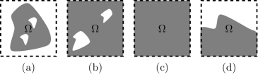
Figure 1: Different families of domains $\Omega$.

As already said, the mathematical study of the Navier-Stokes equations essentially started with the work of Leray (1933), whose method consists of three steps. First the boundary conditions $\boldsymbol{u}^{*}$ and $\boldsymbol{u}_{\infty}$ have to be lifted by an extension $\boldsymbol{a}$ which satisfies the so-called extension condition. The second step is to show the existence of weak solutions in bounded domain. Finally if the domain is unbounded, the third step is to define a sequence of invading bounded domains that coincide in the limit with the unbounded domain and show that the induced sequence of solutions converges in some suitable space. With this strategy, Leray (1933) was able to construct weak solutions in domains with a compact boundary, i.e. cases (a) & (b), if the flux through each connected component of the boundary is zero. If $\Omega$ is bounded and in view of the incompressibility of the fluid, the divergence theorem requires that the total flux through the boundary $\partial\Omega$ is zero, but not that the flux through each connected component of the boundary is zero. If theses fluxes are small enough, the existence of weak solutions was proved by Galdi (1991) in bounded domains and respectively in two and three dimensions by Finn (1961, Theorem 2.6) and Russo (2009) for the unbounded case (b). Without restriction on the magnitude of the fluxes, Korobkov et al. (2014a, b) treated the case of unbounded symmetric exterior domains in both two and three dimensions and recently, Korobkov et al. (2015) proved the existence of weak solutions under no symmetry and smallness assumptions for two-dimensional bounded domains. In the first chapter, we review the above results for small fluxes by proposing a method that includes all the cases in a concise way. In case (c) where $\Omega=\mathbb{R}^{n}$, the method of Leray work without any differences if $n=3$ but cannot be used if $n=2$ to construct weak solutions, whose existence is still an open problem. For the case (d), see Guillod & Wittwer (2015c) and references therein.

If the data are regular enough, Ladyzhenskaya (1959) showed by elliptic regularity that the weak solutions satisfy (LABEL:intro-ns-eq) and (LABEL:intro-ns-bc) in the classical way, which solves the problem (LABEL:intro-ns) if $\Omega$ is bounded. However, if $\Omega$ is unbounded, the validity of the boundary condition at infinity (LABEL:intro-ns-limit) depends drastically on the dimension. In three dimensions, the function space used by Leray, allowed him to show that (LABEL:intro-ns-limit) is satisfied in a weak sense and the existence of uniform pointwise limit was shown later by Finn (1959). However, in two dimensions, the function space used by Leray for the construction of weak solutions does not even ensure that $\boldsymbol{u}$ is bounded at large distances, so that apparently no information on the behavior at infinity $\boldsymbol{u}_{\infty}$ is retained in the limit where the domain becomes infinitely large. The validity of (LABEL:intro-ns-limit) for two-dimensional exterior domains remained completely open until Gilbarg & Weinberger (1974, 1978) partially answered it by showing that either there exists $\boldsymbol{u}_{0}\in\mathbb{R}^{2}$ such that

$$\lim_{\left|\boldsymbol{x}\right|\to\infty}\int_{S^{1}}\left|\boldsymbol{u}-\boldsymbol{u}_{0}\right|^{2}=0\,,\qquad\text{or}\qquad\lim_{\left|\boldsymbol{x}\right|\to\infty}\int_{S^{1}}\left|\boldsymbol{u}\right|^{2}=\infty\,.$$

Nevertheless, the question if the second case of the alternative can be ruled out and if $\boldsymbol{u}_{0}$ coincides with $\boldsymbol{u}_{\infty}$ remains open in general. Later on Amick (1988) showed that if $\boldsymbol{u}^{*}=\boldsymbol{f}=\boldsymbol{0}$, then the first alternative happens, so $\boldsymbol{u}$ is bounded and

$$\lim_{\left|\boldsymbol{x}\right|\to\infty}\boldsymbol{u}=\boldsymbol{u}_{0}\,.$$

In two dimensions, the only results with $\boldsymbol{u}_{\infty}=\boldsymbol{0}$ without assuming small data are obtained by assuming suitable symmetries. Galdi (2004, §3.3) showed that if an exterior domain and the data are symmetric with respect to two orthogonal axes, then there exists a solution satisfying the boundary condition at infinity in the following sense:

$$\lim_{|\boldsymbol{x}|\to\infty}\int_{S^{1}}\left|\boldsymbol{u}\right|^{2}=0\,.$$

This result was improved by Russo (2011, Theorem 7) by only requiring the domain and the data to be invariant under the central symmetry $\boldsymbol{x}\mapsto-\boldsymbol{x}$, and by Pileckas & Russo (2012) by allowing a flux through the boundary. However, all these results rely only on the properties of the subset of symmetric functions in the function space in which weak solutions are constructed, and therefore the decay of the velocity at infinity remains unknown.

weak is a review of the construction of weak solutions in two- and three-dimensional Lipschitz domains for arbitrary large data $\boldsymbol{u}^{*}$ and $\boldsymbol{f}$, provided that the flux of $\boldsymbol{u}^{*}$ through each connected component of $\partial\Omega$ is small. The proofs are based on standard techniques and structured so that all the cases can be treated in one concise way. For unbounded domains, the behavior at infinity of the weak solutions is also reviewed.

In cases (b) & (c), more detailed results can be obtained by linearizing (LABEL:intro-ns-eq) around $\boldsymbol{u}=\boldsymbol{u}_{\infty}$,

$$\Delta\boldsymbol{u}-\boldsymbol{\nabla}p-\boldsymbol{u}_{\infty}\boldsymbol{\cdot}\boldsymbol{\nabla}\boldsymbol{u} =\boldsymbol{f}\,, \boldsymbol{\nabla}\boldsymbol{\cdot}\boldsymbol{u} =\boldsymbol{0}\,,$$ (4)

which is called the Stokes equations if $\boldsymbol{u}_{\infty}=\boldsymbol{0}$ and the Oseen equations if $\boldsymbol{u}_{\infty}\neq\boldsymbol{0}$. The fundamental solution of the Stokes equations behaves like $\left|\boldsymbol{x}\right|^{-1}$ in three dimensions and grows like $\log\left|\boldsymbol{x}\right|$ in two dimensions. However, the fundamental solution of the Oseen equations exhibits a parabolic wake directed in the direction of $\boldsymbol{u}_{\infty}$ in which the decay of the velocity is slower than in the other region. Explicitly in three dimensions the velocity decays like $\left|\boldsymbol{x}\right|^{-1}$ inside the wake and like $\left|\boldsymbol{x}\right|^{-2}$ outside and in two dimensions the decays are $\left|\boldsymbol{x}\right|^{-1/2}$ and $\left|\boldsymbol{x}\right|^{-1}$ respectively inside and outside the wake. In view of these different behaviors of the fundamental solution at infinity, we distinguish the two cases $\boldsymbol{u}_{\infty}\neq\boldsymbol{0}$ and $\boldsymbol{u}_{\infty}=\boldsymbol{0}$.

For $\boldsymbol{u}_{\infty}\neq\boldsymbol{0}$, the estimates of the Oseen equations show that the inversion of the Oseen operator on the nonlinearity leads to a well-posed problem, so a fixed point argument shows the existence of solutions behaving at infinity like the Oseen fundamental solution for small data. This was done by Finn (1965, §4) in three dimensions and by Finn & Smith (1967) in two dimensions. Moreover, in three dimensions, by using results of Finn (1965), Babenko (1973) showed that the solution of (LABEL:intro-ns) found by the method of Leray behaves at infinity like the fundamental solution of the Oseen equations (LABEL:intro-ns-lin), so in particular $\boldsymbol{u}-\boldsymbol{u}_{\infty}=O(\left|\boldsymbol{x}\right|^{-1})$ at infinity. In two dimensions, by the results of Smith (1965, §4) and Galdi (2011, Theorem XII.8.1), one has that if $\boldsymbol{u}$ is a solution of (LABEL:intro-ns), then $\boldsymbol{u}$ is asymptotic to the Oseen fundamental solution, so $\boldsymbol{u}-\boldsymbol{u}_{\infty}=O(\left|\boldsymbol{x}\right|^{-1/2})$. However, it is still not known if the solutions constructed by the method of Leray (1933) satisfy (LABEL:intro-ns-limit) in two dimensions and therefore if they coincide with the solutions found by Finn & Smith (1967). These results on the asymptotic behavior of weak solutions will be reviewed at the end of weak.

From now one, we consider the case where $\boldsymbol{u}_{\infty}=\boldsymbol{0}$. As already said, in three dimensions, the function spaces imply the validity of (LABEL:intro-ns-limit) even if $\boldsymbol{u}_{\infty}=\boldsymbol{0}$, whereas in two dimensions, all the available results are obtained by assuming suitable symmetries (Galdi, 2004; Yamazaki, 2009, 2011; Pileckas & Russo, 2012) or specific boundary conditions (Hillairet & Wittwer, 2013). Yamazaki (2011) showed the existence and uniqueness of solutions for small data in an exterior domain provided the domain and the data are invariant under four axes of symmetries with an angle of $\pi/4$ between them. In the exterior of a disk, Hillairet & Wittwer (2013) proved the existence of solutions that decay like $\left|\boldsymbol{x}\right|^{-1}$ at infinity provided that the boundary condition on the disk is close to $\mu\boldsymbol{e}_{r}$ for $\left|\mu\right|>\sqrt{48}$. To our knowledge, these last two results together with the exact solutions found by Hamel (1917); Guillod & Wittwer (2015b) are the only ones showing the existence of solutions in two-dimensional exterior domains satisfying (LABEL:intro-ns-limit) with $\boldsymbol{u}_{\infty}=\boldsymbol{0}$ and a known decay rate at infinity.

We now analyze the implications of the decay of the velocity on the linear and nonlinear terms and on the net force. For simplicity, we consider in this paragraph the domain $\Omega=\mathbb{R}^{n}$ and a source force $\boldsymbol{f}$ with compact support, but the following considerations can be extended to the case where $\Omega$ has a compact boundary and $\boldsymbol{f}$ decays fast enough. A fundamental quantity is the net force $\boldsymbol{F}$ which has a simple expression due to the previous hypothesis,

$$\boldsymbol{F}=\int_{\mathbb{R}^{n}}\boldsymbol{f}\,.$$

If the net force is nonzero, the solution of the Stokes equations has a velocity field that decays like $\left|\boldsymbol{x}\right|^{-1}$ for $n=3$ and that grows like $\log\left|\boldsymbol{x}\right|$ for $n=2$. This is the well-known Stokes paradox. By power counting, if the velocity decays like $\left|\boldsymbol{x}\right|^{-\alpha}$, we have

$$\boldsymbol{u} \sim\left|\boldsymbol{x}\right|^{-\alpha}\,, \boldsymbol{\nabla}\boldsymbol{u} \sim\left|\boldsymbol{x}\right|^{-\alpha-1}\,, \Delta\boldsymbol{u} \sim\left|\boldsymbol{x}\right|^{-\alpha-2}\,, \boldsymbol{u}\boldsymbol{\cdot}\boldsymbol{\nabla}\boldsymbol{u} \sim\left|\boldsymbol{x}\right|^{-2\alpha-1}\,,$$ (5)

and therefore the Navier-Stokes equations (LABEL:intro-ns-eq) are essentially linear (subcritial) for $\alpha>1$, are critical for $\alpha=1$, and highly nonlinear (supercritical) for $\alpha<1$. However, since the net force is a conserved quantity, we have for $\boldsymbol{f}$ with compact support and $R$ big enough:

$$\boldsymbol{F}=\int_{\mathbb{R}^{n}}\boldsymbol{f}=\int_{\partial B(\boldsymbol{0},R)}\mathbf{T}\boldsymbol{n}\,,$$

where $\mathbf{T}$ is the stress tensor including the convective part, $\mathbf{T}=\boldsymbol{\nabla}\boldsymbol{u}+\left(\boldsymbol{\nabla}\boldsymbol{u}\right)^{T}-p\,\boldsymbol{1}-\boldsymbol{u}\otimes\boldsymbol{u}$ and $B(\boldsymbol{0},R)$ the open ball of radius $R$ centered at the origin. Again by power counting, if $\boldsymbol{u}$ satisfies (LABEL:decay), we obtain that $\mathbf{T}\sim\left|\boldsymbol{x}\right|^{-\min(\alpha+1,2\alpha)}$, so if $2\alpha>n-1$, the limit $R\to\infty$ vanishes and $\boldsymbol{F}=\boldsymbol{0}$. Consequently, in three dimensions, $\alpha=1$ is the critical case for the equations as well as for the net force, whereas in two dimensions, the equations have to be supercritical if we want to generate a nonzero net force. If the net force vanishes, the solution of the Stokes equations decays like $\left|\boldsymbol{x}\right|^{-2}$ in three dimensions, so the problem is subcritical and like $\left|\boldsymbol{x}\right|^{-1}$ in two dimensions, which is the critical regime. The different regimes are described in summary-decays. Therefore, the problem is critical in three dimensions if $\boldsymbol{F}\neq\boldsymbol{0}$ and in two dimensions if $\boldsymbol{F}=\boldsymbol{0}$. In both of these cases, inverting the Stokes operator on the nonlinearity, which by power counting decays like $\left|\boldsymbol{x}\right|^{-3}$, leads to a solution decaying like $\left|\boldsymbol{x}\right|^{-1}\log\left|\boldsymbol{x}\right|$. Therefore, the Stokes system is ill-posed in this critical setting and the leading term at infinity cannot be the Stokes fundamental solution. In three dimensions this was proven by Deuring & Galdi (2000, Theorem 3.1) and in two dimensions this is proven in link-Stokes-NS.

We now discuss the critical cases in more details. In three dimensions, by using an idea of Nazarov & Pileckas (2000, Theorem 3.2), Korolev & Šverák (2011) proved by a fixed point argument that for small data the asymptotic behavior is given by a class of exact solutions found by Landau (1944). The Landau solutions are a family of exact and explicit solutions ${\boldsymbol{U}\!}_{\boldsymbol{F}}$ of (LABEL:intro-ns) in $\mathbb{R}^{3}\setminus\left\{\boldsymbol{0}\right\}$ parameterized by $\boldsymbol{F}\in\mathbb{R}^{3}$ and corresponding, in the sense of distributions, to $\boldsymbol{f}(\boldsymbol{x})=\boldsymbol{F}\delta^{3}(\boldsymbol{x})$, so having a net force $\boldsymbol{F}$. Moreover, these are the only solutions that are invariant under the scaling symmetry, i.e. such that $\lambda\boldsymbol{u}(\lambda\boldsymbol{x})=\boldsymbol{u}(\boldsymbol{x})$ for all $\lambda>0$ (Šverák, 2011). Given this candidate for the asymptotic expansion of the solution up to the critical decay, the second step is to define $\boldsymbol{u}={\boldsymbol{U}\!}_{\boldsymbol{F}}+\boldsymbol{v}$, so that the Navier-Stokes equations (LABEL:intro-ns) become

$$\Delta\boldsymbol{v}-\boldsymbol{\nabla}q ={\boldsymbol{U}\!}_{\boldsymbol{F}}\boldsymbol{\cdot}\boldsymbol{\nabla}\boldsymbol{v}+\boldsymbol{v}\boldsymbol{\cdot}\boldsymbol{\nabla}{\boldsymbol{U}\!}_{\boldsymbol{F}}+\boldsymbol{v}\boldsymbol{\cdot}\boldsymbol{\nabla}\boldsymbol{v}+\boldsymbol{g}\,, \boldsymbol{\nabla}\boldsymbol{\cdot}\boldsymbol{u} =0\,, \lim_{|\boldsymbol{x}|\to\infty}\boldsymbol{u} =\boldsymbol{0}\,,$$

where the resulting source term $\boldsymbol{g}$ has zero mean, which lifts the compatibility condition of the Stokes problem related to the net force. Since ${\boldsymbol{U}\!}_{\boldsymbol{F}}$ is bounded by $\left|\boldsymbol{x}\right|^{-1}$, the cross term ${\boldsymbol{U}\!}_{\boldsymbol{F}}\boldsymbol{\cdot}\boldsymbol{\nabla}\boldsymbol{v}+\boldsymbol{v}\boldsymbol{\cdot}\boldsymbol{\nabla}{\boldsymbol{U}\!}_{\boldsymbol{F}}$ is a critical perturbation of the Stokes operator. Therefore this term can be put together with the nonlinearity in order to perform a fixed point argument on a space where $\boldsymbol{v}$ is bounded by $\left|\boldsymbol{x}\right|^{-2+\varepsilon}$ for some $\varepsilon>0$. This argument leads to the existence of solutions satisfying

$$\boldsymbol{u}={\boldsymbol{U}\!}_{\boldsymbol{F}}+O(\left|\boldsymbol{x}\right|^{-2+\varepsilon})\,,$$

provided $\boldsymbol{f}$ is small enough. Therefore, the key idea of this method is to find the asymptotic term that lifts the compatibility condition corresponding to the net force $\boldsymbol{F}$. If net force is zero, the solution of the Stokes equations in three dimensions decays like $\left|\boldsymbol{x}\right|^{-2}$, so we are in the subcritical regime and everything is governed by the linear part of the equation, i.e. the Stokes equations.

In two dimensions and if $\boldsymbol{F}=\boldsymbol{0}$, the solution of the Stokes equations again decays like $\left|\boldsymbol{x}\right|^{-1}$, and therefore we are also in the critical case. In strong-compatibility we determine the three additional compatibility conditions on the data needed so that the solution of the Stokes equations decay faster than $\left|\boldsymbol{x}\right|^{-1}$. Once this is known, we can use a fixed point argument in order to obtain the existence of solutions decaying faster than $\left|\boldsymbol{x}\right|^{-1}$ for small data satisfying three compatibility conditions. Moreover, these compatibility conditions can be automatically fulfilled by assuming suitable discrete symmetries, which will improve the results of Yamazaki (2011). In strong-compatibility, we also show how to lift the compatibility condition corresponding to the net torque $M$ with the solution $M\left|\boldsymbol{x}\right|^{-2}\boldsymbol{x}^{\perp}$, however two compatibility conditions not related to invariant quantities remain.

In link-Stokes-NS, we prove that the two solutions of the Stokes equations decaying like $\left|\boldsymbol{x}\right|^{-1}$ and which are given by the two remaining compatibility conditions cannot be the asymptote of any solutions of the Navier-Stokes equations in two-dimensions. By analogy with the three-dimensional case where the asymptote is given by the Landau solution which is scale-invariant, we can look for a scale-invariant solution to describe the asymptotic behavior also in two dimensions. As proved by Šverák (2011), the scale-invariant solutions of the Navier-Stokes equations are given by the exact solutions found by Hamel (1917, §6). These solutions are parameterized by the flux $\Phi\in\mathbb{R}$, an angle $\theta_{0}$, and a discrete parameter $n$. As explained by Šverák (2011, §5), they are far from the Stokes solutions decaying like $\left|\boldsymbol{x}\right|^{-1}$, so cannot be used to lift the compatibility conditions of the Stokes equations. In an attempt to obtain the correct asymptotic behavior, Guillod & Wittwer (2015b) defined the notion of a scale-invariant solution up to a rotation, i.e. a solution that satisfies

$$\boldsymbol{u}(\boldsymbol{x})=\mathrm{e}^{\lambda}\mathbf{R}_{\kappa\lambda}\boldsymbol{u}(\mathrm{e}^{\lambda}\mathbf{R}_{-\kappa\lambda}\boldsymbol{x})\,,$$

for some $\kappa\in\mathbb{R}$, where $\mathbf{R}_{\vartheta}$ is the rotation matrix of angle $\vartheta$. This is a combination of the scaling and rotational symmetries. The scale-invariant solutions up to a rotation of the two-dimensional Navier-Stokes equations in $\mathbb{R}^{2}\setminus\left\{\boldsymbol{0}\right\}$ are parameterized by the flux $\Phi\in\mathbb{R}$, a parameter $\kappa\in\mathbb{R}$, an angle $\theta_{0}$, and a discrete parameter $n$. These solutions generalize the solutions found by Hamel (1917, §6) and exhibit a spiral behavior as shown in intro-hamel-new. However, at zero-flux, these new exact solutions have only two free parameters, and are therefore not sufficient to lift the three compatibility conditions of the Stokes equations required for a decay of the velocity strictly faster than the critical decay $\left|\boldsymbol{x}\right|^{-1}$. Nevertheless, these exact solutions show that the asymptotic behavior of the solutions in the case where $\boldsymbol{F}=\boldsymbol{0}$ are highly nontrivial, since by choosing a suitable boundary condition $\boldsymbol{u}^{*}$ for an exterior domain or source force $\boldsymbol{f}$ if $\Omega=\mathbb{R}^{2}$, it is easy to construction a solution that is equal to any of these exact solutions, at least at large distances. Therefore the determination of the general asymptotic behavior of the two-dimensional Navier-Stokes equations with zero net force is still open and the numerical simulations presented in wake-sim seem to indicate that the asymptotic behavior is quite complicated.

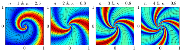
Figure 2: The exact solutions found by Guillod & Wittwer (2015b) with zero flux are parametrized by a discrete parameter $n$ and a real parameter $\kappa$.

Finally, we discuss the supercritical case, that is to say the two-dimensional Navier-Stokes equations for a nonzero net force $\boldsymbol{F}\neq\boldsymbol{0}$. By assuming that the decay of the solution is homogeneous, the previous power counting argument shows that the solution cannot decay faster than $\left|\boldsymbol{x}\right|^{-1/2}$. By assuming that the velocity field has an homogeneous decay like $\left|\boldsymbol{x}\right|^{-1/2}$, we obtain that this leading term has to be a solution of the Euler equations. Such a solution of the Euler equations generating a nonzero net force $\boldsymbol{F}$ exists. However this cannot be the asymptotic behavior of the Navier-Stokes equations at least for small data, because the solution will have a big flux $\Phi\leq-3\pi$. This analysis is shown in asy-euler.

The idea to determine the correct asymptotic behavior is to make an ansatz such that at large distances, parts of the linear and nonlinear terms of the equation remain both dominant unlike for the previous attempt where only the nonlinear part had dominant terms. More precisely, Guillod & Wittwer (2015a) consider an inhomogeneous ansatz, whose decay and inhomogeneity are fixed by the requirement that parts of the linearity and nonlinearity remain at large distances and that net force is nonzero. The analysis in Guillod & Wittwer (2015a) was done in Cartesian coordinates which are not very adapted to this problem. In asy-wake, we use a conformal change of coordinates to introduce the inhomogeneity which makes the analysis much simpler and intuitive. This leads to a solution $\left({\boldsymbol{U}\!}_{\boldsymbol{F}},P_{\boldsymbol{F}}\right)$ of the Navier-Stokes equations in $\mathbb{R}^{2}$ with some $\boldsymbol{f}=\left(O(\left|\boldsymbol{x}\right|^{-7/3}),O(\left|\boldsymbol{x}\right|^{-8/3})\right)$ at infinity. This solution generates a net force $\boldsymbol{F}$ and is a candidate for the general asymptotic behavior in the case $\boldsymbol{F}\neq\boldsymbol{0}$. In polar coordinates, the velocity field has the following decay at infinity,

$${\boldsymbol{U}\!}_{\boldsymbol{F}}=\frac{2a^{2}}{3r^{1/3}}\operatorname{sech}^{2}\left(a\sin\left(\frac{\theta-\theta_{0}}{3}\right)r^{1/3}\right)\frac{\boldsymbol{F}}{\left|\boldsymbol{F}\right|}+O(r^{-2/3})\,,$$ (6)

where

$$\theta_{0} =\arg(-F_{1}-\mathrm{i}F_{2})\,, a =\left(\frac{9\left|\boldsymbol{F}\right|}{16}\right)^{1/3}\,.$$

This solution is represented in intro-ansatz and has a wake behavior: inside the wake characterized by $\left|\theta-\theta_{0}\right|r^{1/3}\leq 1$, the velocity decays like $\left|\boldsymbol{x}\right|^{-1/3}$ and outside the wake like $\left|\boldsymbol{x}\right|^{-2/3}$. This time, the asymptotic expansion does not have a flux, and moreover numerical simulations (see intro-wake) indicate that this is most probably the correct asymptotic behavior if $\boldsymbol{F}\neq\boldsymbol{0}$. In the last part of wake-sim, we will perform systematic numerical simulations based on the analysis of the Stokes equations and the results of strong-compatibility,link-Stokes-NS. More precisely, when the net force is nonzero, the asymptotic behavior is given by ${\boldsymbol{U}\!}_{\boldsymbol{F}}$, however when the net force is vanishing the asymptotic behavior seems to be much less universal. In some regime, the asymptote is given by a double wake ${\boldsymbol{U}\!}_{\boldsymbol{F}}+{\boldsymbol{U}\!}_{-\boldsymbol{F}}$ so that the net force is effectively zero (see intro-wake-double), in some other regime by the harmonic solution $\mu\boldsymbol{e}_{\theta}/r$ , and finally can also be the exact scale -invariant solution up to a rotation discussed in Guillod & Wittwer (2015b). The presence of the double wake is surprising, because intuitively on would expect that the solution should behave like the Stokes solution, i.e. like $\left|\boldsymbol{x}\right|^{-1}$ and not like $\left|\boldsymbol{x}\right|^{-1/3}$, since we are in the critical case as in three dimensions where the asymptote is the Landau (1944) solution. Finally, in wake-multiple we also show numerically that three or more wakes can be produced, but only for large data. The decays of the Stokes and Navier-Stokes equations as well as their asymptotes are summarized in summary-decays.

Acknowledgment

The author would like to thank Peter Wittwer for many useful discussions and comments on the subject of this work as well as Matthieu Hillairet for fruitful discussions and for having pointed out the exact solution of the Euler equations given in (LABEL:euler-sol).

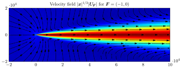
Figure 3: The solution ${\boldsymbol{U}\!}_{\boldsymbol{F}}$ is multiplied by $\left|\boldsymbol{x}\right|^{1/3}$ in order to highlight its decay properties. Inside a wake characterized by $\left|\theta\right|r^{1/3}\leq 1$, ${\boldsymbol{U}\!}_{\boldsymbol{F}}$ decays like $\left|\boldsymbol{x}\right|^{-1/3}$ inside the wake, whereas it decays like $\left|\boldsymbol{x}\right|^{-2/3}$ outside the wake region.

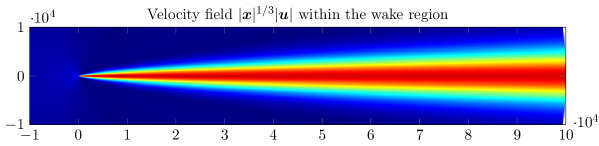
Figure 4: Numerical simulation of the Navier-Stokes equations with $\boldsymbol{F}\neq\boldsymbol{0}$. The velocity field is asymptotic to ${\boldsymbol{U}\!}_{\boldsymbol{F}}$ defined by (LABEL:intro-exact-wake) with very high precision.

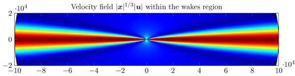
Figure 5: Numerical simulation of the Navier-Stokes equations with $\boldsymbol{F}=\boldsymbol{0}$ for a specific choice of the boundary conditions. The velocity field is only bounded by $\left|\boldsymbol{x}\right|^{-1/3}$.

Table 1: Summary of the different properties of the Stokes and Navier-Stokes equations in $\mathbb{R}^{n}$. In every dimension, the critical decay of the Navier-Stokes equations is given by $\left|\boldsymbol{x}\right|^{-1}$ and is drawn in yellow. The decays that make the equations subcritical are drawn in green and the ones that are supercritical are shown in red. As shown on page 1, the critical decay for having a nonzero net force is $\left|\boldsymbol{x}\right|^{-1/2}$ in two dimensions and $\left|\boldsymbol{x}\right|^{-1}$ in three dimensions. The results of the two-dimensional cases are based on Guillod & Wittwer (2015a, b) and on the results of wake-sim. In three dimensions, the results were proven by Korolev & Šverák (2011).

1 Notations

For the reader’s convenience, we collect here the most frequently used symbols:

$\lesssim$	less than up to a constant: $a\lesssim b$ means $a\leq Cb$ for some $C>0$
$n$	dimension of the underlying space
$\boldsymbol{x}$	position: $\boldsymbol{x}=(x_{1},\dots,x_{n})$
$\boldsymbol{e}_{i}$	unit vector in the direction $i$
$r$	radial polar coordinate: $r=|\boldsymbol{x}|$
$\theta$	angular polar coordinate: $\theta=\arg(x_{1}+\mathrm{i}x_{2})\in(-\pi;\pi]$
$B(\boldsymbol{x},R)$	open ball of radius $R$ centered at $\boldsymbol{x}$
$\Omega$	region of flow
$\partial\Omega$	boundary of the domain $\Omega$
$\boldsymbol{n}$	normal outgoing unit vector to the boundary $\partial\Omega$
$\boldsymbol{v}$	vector: $\boldsymbol{v}=(v_{1},\dots,v_{n})$
$|\boldsymbol{v}|$	Euclidean norm of the vector $\boldsymbol{v}$: $|\boldsymbol{v}|^{2}=\sum_{i=1}^{n}v_{i}^{2}$
$\boldsymbol{v}^{\perp}$	orthogonal of the two-dimensional vector $\boldsymbol{v}=(v_{1},v_{2})$: $\boldsymbol{v}^{\perp}=(-v_{2},v_{1})$
$\boldsymbol{v}_{1}\boldsymbol{\cdot}\boldsymbol{v}_{2}$	scalar product between $\boldsymbol{v}_{1}$ and $\boldsymbol{v}_{2}$
$\boldsymbol{v}_{1}\boldsymbol{\wedge}\boldsymbol{v}_{2}$	cross product between the three-dimensional vectors $\boldsymbol{v}_{1}$ and $\boldsymbol{v}_{2}$
$\mathbf{A}$	second-order tensor field: $\boldsymbol{A}=(A_{ij})_{i,j=1,\dots,n}$
$\mathbf{A}:\mathbf{B}$	contraction of the tensors $\mathbf{A}$ and $\mathbf{B}$: $\mathbf{A}:\mathbf{B}=\sum_{i,j=1}^{n}A_{ij}B_{ij}$
$\varphi$	scalar field: $\varphi(x)$
$\boldsymbol{\varphi}$	vector field: $\left(\varphi_{1}(\boldsymbol{x}),\dots,\varphi_{n}(\boldsymbol{x})\right)$
$\boldsymbol{\nabla}\varphi$	gradient of the scalar field $\varphi$: $\boldsymbol{\nabla}\varphi=(\partial_{1}\varphi,\dots,\partial_{n}\varphi)$
$\boldsymbol{\nabla}\boldsymbol{\cdot}\boldsymbol{\varphi}$	divergence of the vector field $\boldsymbol{\varphi}$: $\boldsymbol{\nabla}\boldsymbol{\cdot}\boldsymbol{\varphi}=\sum_{i=1}^{n}\partial_{i}\varphi_{i}$
$\boldsymbol{\nabla}\boldsymbol{\wedge}\boldsymbol{\varphi}$	curl of the three-dimensional vector field $\boldsymbol{\varphi}$
$\boldsymbol{\nabla}\wedge\varphi$	curl of the scalar field $\varphi$: $\boldsymbol{\nabla}\wedge\varphi=\boldsymbol{\nabla}^{\perp}\varphi=(-\partial_{2}\varphi,\partial_{1}\varphi)$
$\boldsymbol{u}$	velocity field
$p$	pressure field
$\omega$	vorticity field: $\omega=\boldsymbol{\nabla}\boldsymbol{\wedge}\boldsymbol{u}$
$\psi$	stream function: $\boldsymbol{u}=\boldsymbol{\nabla}\wedge\psi$

2 Symmetries of the Navier-Stokes equations

The aim is to determine all the infinitesimal symmetries that leave the homogeneous Navier-Stokes equations in $\mathbb{R}^{n}$ invariant. The symmetries of the time-dependent Navier-Stokes equations were determined by Lloyd (1981). It is not completely obvious that the symmetries of the stationary case are given by the time-independent symmetries of the time-dependent case only. The following proposition establishes that this is actually the case:

Proposition 1.1.

For $n=2,3$, the only infinitesimal symmetries of the type

$$\boldsymbol{x}\mapsto \boldsymbol{x}+\varepsilon\boldsymbol{\xi}(\boldsymbol{u},p,\boldsymbol{x})\,, \left(\boldsymbol{u},p\right) \mapsto\left(\boldsymbol{u},p\right)+\boldsymbol{\eta}(\boldsymbol{u},p,\boldsymbol{x})\,,$$ (7)

i.e. generated by

$$X=\boldsymbol{\xi}\boldsymbol{\cdot}\boldsymbol{\nabla}_{\boldsymbol{x}}+\boldsymbol{\eta}\boldsymbol{\cdot}\boldsymbol{\nabla}_{(\boldsymbol{u},p)}\,,$$

which leave the homogeneous Navier-Stokes equations in $\mathbb{R}^{n}$ invariant are:

1. The translations

   $$\boldsymbol{x}\mapsto\boldsymbol{x}+\boldsymbol{\delta}\,,$$

   where $\boldsymbol{\delta}\in\mathbb{R}^{n}$, whose generator is given by

   $$X=\frac{\boldsymbol{\delta}}{\left|\boldsymbol{\delta}\right|}\boldsymbol{\cdot}\boldsymbol{\nabla}_{\boldsymbol{x}}\,.$$

2. The rotations

   $$\boldsymbol{u}(\boldsymbol{x}) \mapsto\mathbf{R}^{-1}\boldsymbol{u}(\mathbf{R}\boldsymbol{x})\,, p(\boldsymbol{x}) \mapsto p(\mathbf{R}\boldsymbol{x})\,,$$

   for $\mathbf{R}\in\text{SO}(n)$, where the $n(n-1)/2$ generators are given in terms of the lie algebra $\mathfrak{so}(n)$. For example for $n=2$,

   $$X=\boldsymbol{x}^{\perp}\boldsymbol{\cdot}\left(\boldsymbol{\nabla}_{\boldsymbol{x}}+\boldsymbol{\nabla}_{\boldsymbol{u}}\right)\,.$$

3. The scaling symmetry,

   $$\boldsymbol{u}(\boldsymbol{x}) \mapsto\mathrm{e}^{\lambda}\boldsymbol{u}(\mathrm{e}^{\lambda}\boldsymbol{x})\,, p(\boldsymbol{x}) =\mathrm{e}^{2\lambda}p(\mathrm{e}^{\lambda}\boldsymbol{x})\,,$$

   for $\lambda\in\mathbb{R}$, which corresponds to

   $$X=\boldsymbol{x}\boldsymbol{\cdot}\boldsymbol{\nabla}_{\boldsymbol{x}}-\boldsymbol{u}\boldsymbol{\cdot}\boldsymbol{\nabla}_{\boldsymbol{u}}-2p\partial_{p}\,.$$

4. The addition of a constant $c$ to the pressure,

   $$p\mapsto p+c\,,$$

   for $c\in\mathbb{R}$, which corresponds to

   $$X=\partial_{p}\,.$$

Proof.

We use the same method as Lloyd (1981), which is explained in details by Eisenhart (1933). First of all we write the Navier-Stokes equations as $\boldsymbol{L}=\boldsymbol{0}$, where

$$\boldsymbol{L}=\begin{pmatrix}\Delta\boldsymbol{u}-\boldsymbol{\nabla}p-\boldsymbol{u}\boldsymbol{\cdot}\boldsymbol{\nabla}\boldsymbol{u}\\ \boldsymbol{\nabla}\boldsymbol{\cdot}\boldsymbol{u}\end{pmatrix}\,,$$

and define $\boldsymbol{v}=\left(\boldsymbol{u},p\right)$. Since $\boldsymbol{L}$ is a second order differential operator, we have to compute the transformations of the first and second derivatives. We have

$$\partial_{i}\mapsto\partial_{i}-\varepsilon\frac{\mathrm{d}\boldsymbol{\xi}}{\mathrm{d}x_{i}}\boldsymbol{\cdot}\boldsymbol{\nabla}\,,$$

so that

$$D^{\alpha}\boldsymbol{v}\mapsto D^{\alpha}\boldsymbol{v}+\varepsilon\boldsymbol{\eta}^{\alpha}\,,$$

where $\boldsymbol{\eta}^{\alpha}$ is defined by recursion through

$$\boldsymbol{\eta}^{(\alpha,\beta)}=\frac{\mathrm{d}\boldsymbol{\eta}^{\beta}}{\mathrm{d}x_{\alpha}}-\frac{\mathrm{d}\boldsymbol{\xi}}{\mathrm{d}x_{\alpha}}\boldsymbol{\cdot}\boldsymbol{\nabla}D^{\beta}\boldsymbol{v}\,,$$

where $\alpha$ and $\beta$ are multi-indices with $\left|\alpha\right|=1$. We consider the second extension of $X$,

$$X_{2}=\boldsymbol{\xi}\boldsymbol{\cdot}\boldsymbol{\nabla}_{\boldsymbol{x}}+\sum_{\left|\alpha\right|\leq 2}\boldsymbol{\eta}^{\alpha}\boldsymbol{\cdot}\boldsymbol{\nabla}_{D^{\alpha}\boldsymbol{v}}\,.$$

Then the Navier-Stokes system admits the symmetry (LABEL:symmetries-epsilon) if and only if $X_{2}\boldsymbol{L}=\boldsymbol{0}$ whenever $\boldsymbol{L}=\boldsymbol{0}$. The idea of the proof is the following: we solve $\boldsymbol{L}=\boldsymbol{0}$ for $\boldsymbol{\nabla}p$ and $\partial_{1}u_{1}$, and substitute this into $X_{2}\boldsymbol{L}=\boldsymbol{0}$. By grouping similar terms involving $\boldsymbol{v}$ and its derivatives, we can obtain a list of linear partial differential equations for $\boldsymbol{\xi}$ and $\boldsymbol{\eta}$. By using a computer algebra system, we obtain the explicit list of partial differential equations for $\boldsymbol{\xi}$ and $\boldsymbol{\eta}$. For $n=2$, the general solution is given by

$$\boldsymbol{\xi} =\boldsymbol{\delta}+\lambda\boldsymbol{x}+r\boldsymbol{x}^{\perp}\,,$$

$$\left(\eta_{1},\eta_{2}\right) =-\lambda\boldsymbol{u}+r\boldsymbol{x}^{\perp}$$

$$\eta_{3} =-2p\lambda+c\,,$$

where $\boldsymbol{\delta}\in\mathbb{R}^{2}$ and $\lambda,r,c\in\mathbb{R}$. For $n=3$, we have similar results, except that there are three different rotations. ∎

In additions to the four infinitesimal symmetries listed in symmetries, the Navier-Stokes equations are also invariant under discrete symmetries. They are invariant under the central symmetry

$$\boldsymbol{x} \mapsto-\boldsymbol{x}\,, \boldsymbol{u} \mapsto-\boldsymbol{u}\,,$$ (8)

and under the reflections with respect to an axis or a plane. For example, the reflection with respect to the first coordinate $x_{1}$ is given by

$$\boldsymbol{x}=\left(x_{1},\tilde{\boldsymbol{x}}\right) \mapsto\left(-x_{1},\tilde{\boldsymbol{x}}\right)\,, \boldsymbol{u}=\left(u_{1},\tilde{\boldsymbol{u}}\right) \mapsto\left(-u_{1},\tilde{\boldsymbol{u}}\right)\,.$$ (9)

This corresponds to the reflection with respect to the $x_{2}$-axis for $n=2$ and with respect to the $x_{2}x_{3}$-plane for $n=3$.

3 Invariant quantities of the Navier-Stokes equations

We consider the stationary Navier-Stokes equations (LABEL:intro-ns-eq) in a sufficiently smooth bounded domain $\Omega\subset\mathbb{R}^{n}$, $n=2,3$. For clarity, we add a source-term $g$ in the divergence equation, so we consider

$$\Delta\boldsymbol{u}-\boldsymbol{\nabla}p =\boldsymbol{\nabla}\boldsymbol{\cdot}\left(\boldsymbol{u}\otimes\boldsymbol{u}\right)+\boldsymbol{f}\,, \boldsymbol{\nabla}\boldsymbol{\cdot}\boldsymbol{u} =g\,,$$ (10)

which is equal to (LABEL:intro-ns-eq) if $g=0$. The aim is to show that the only invariant quantities in a sense defined below, are the flux, the net force, and the net torque.

Definition 1.2 (invariant quantity).

For two functions $\boldsymbol{\Lambda}\in C^{\infty}(\Omega,\mathbb{R}^{n+1})$ and $\Lambda\in C^{\infty}(\Omega,\mathbb{R})$ we consider the functional

$$I[\boldsymbol{f},g]=\int_{\Omega}\left(\boldsymbol{\Lambda}\boldsymbol{\cdot}\boldsymbol{f}+\Lambda g\right)\,.$$

The functional $I[\boldsymbol{f},g]$ is an invariant quantity if it can be expressed in terms of an integral on $\partial\Omega$, i.e. such that there exists a function $\boldsymbol{\lambda}\in C^{\infty}(\mathbb{R}^{n+1},\mathbb{R}^{n})$ with

$$I[\boldsymbol{f},g]=\int_{\partial\Omega}\boldsymbol{\lambda}[\boldsymbol{u},p]\boldsymbol{\cdot}\boldsymbol{n}\,,$$

for any smooth $\boldsymbol{u}$, $p$, $\boldsymbol{f}$ and $g$ satisfying (LABEL:invariant-ns).

Remark 1.3.

The name invariant comes from the fact that if for example $\boldsymbol{u},p,\boldsymbol{f},g$ satisfy (LABEL:invariant-ns) in $\mathbb{R}^{n}$, with $\boldsymbol{f},g$ having support in a bounded set $B$, then the quantity $I[\boldsymbol{f},g]$ does not depend on the domain of integration $\Omega$ as soon as $B\subset\Omega$, and in particular $\int_{\partial\Omega}\boldsymbol{\lambda}[\boldsymbol{u},p]\boldsymbol{\cdot}\boldsymbol{n}$ is independent of the choice of any smooth closed curve or surface $\partial\Omega$ that encircles $B$.

Proposition 1.4.

The only invariant quantities (that are not linearly related) are the flux $\Phi\in\mathbb{R}$, the net force $\boldsymbol{F}\in\mathbb{R}^{n}$, and the net torque $M\in\mathbb{R}$ if $n=2$ and $\boldsymbol{M}\in\mathbb{R}^{3}$ if $n=3$, which are given by

$$\Phi =\int_{\Omega}g=\int_{\partial\Omega}\boldsymbol{u}\boldsymbol{\cdot}\boldsymbol{n}\,, \boldsymbol{F} =\int_{\Omega}\boldsymbol{f}=\int_{\partial\Omega}\mathbf{T}\boldsymbol{n}\,, M\text{ or }\boldsymbol{M} =\int_{\Omega}\boldsymbol{x}\boldsymbol{\wedge}\boldsymbol{f}=\int_{\partial\Omega}\boldsymbol{x}\boldsymbol{\wedge}\mathbf{T}\boldsymbol{n}\,,$$

where $\mathbf{T}$ is the stress tensor including the convective part,

$$\mathbf{T}=\boldsymbol{\nabla}\boldsymbol{u}+\left(\boldsymbol{\nabla}\boldsymbol{u}\right)^{T}-p\,\mathbf{1}-\boldsymbol{u}\otimes\boldsymbol{u}\,.$$ (11)

Proof.

The Navier-Stokes equation (LABEL:invariant-ns) can be written as

$$\boldsymbol{\nabla}\boldsymbol{\cdot}\mathbf{T} =\boldsymbol{f}\,, \boldsymbol{\nabla}\boldsymbol{\cdot}\boldsymbol{u} =g\,.$$

For two general functions $\boldsymbol{\Lambda}$ and $\Lambda$, and a solution of the previous equation, we have

$$I[\boldsymbol{f},g] =\int_{\Omega}\left(\boldsymbol{\Lambda}\boldsymbol{\cdot}\boldsymbol{f}+\Lambda g\right)=\int_{\Omega}\boldsymbol{\Lambda}\boldsymbol{\cdot}\boldsymbol{\nabla}\boldsymbol{\cdot}\mathbf{T}+\int_{\Omega}\Lambda\boldsymbol{\nabla}\boldsymbol{\cdot}\boldsymbol{u}$$

$$=\int_{\Omega}\boldsymbol{\nabla}\boldsymbol{\cdot}\left(\mathbf{T}\boldsymbol{\Lambda}\right)-\int_{\Omega}\boldsymbol{\nabla}\boldsymbol{\Lambda}:\mathbf{T}+\int_{\Omega}\boldsymbol{\nabla}\boldsymbol{\cdot}\left(\Lambda\boldsymbol{u}\right)-\int_{\Omega}\boldsymbol{\nabla}\Lambda\boldsymbol{\cdot}\boldsymbol{u}$$

$$=\int_{\partial\Omega}\left(\mathbf{T}\boldsymbol{\Lambda}+\Lambda\boldsymbol{u}\right)\boldsymbol{\cdot}\boldsymbol{n}-\int_{\Omega}\left(\boldsymbol{\nabla}\boldsymbol{\Lambda}:\mathbf{T}+\boldsymbol{\nabla}\Lambda\boldsymbol{\cdot}\boldsymbol{u}\right)\,.$$

Now we determine in which cases the integral over $\Omega$ vanishes,

$$\int_{\Omega}\left(\boldsymbol{\nabla}\boldsymbol{\Lambda}:\mathbf{T}+\boldsymbol{\nabla}\Lambda\boldsymbol{\cdot}\boldsymbol{u}\right)=0$$

for all $\boldsymbol{u},p,\boldsymbol{f},g$ satisfying (LABEL:invariant-ns). Since this integral does not depend on $\boldsymbol{f}$ and $g$, we can choose $\boldsymbol{u}\in C^{\infty}(\Omega,\mathbb{R}^{n})$ and $p\in C^{\infty}(\Omega,\mathbb{R})$ arbitrarily, and therefore the tensor $\mathbf{T}$ is an arbitrary symmetric tensor. Consequently, we obtain the conditions

$$\int_{\Omega}\boldsymbol{\nabla}\boldsymbol{\Lambda}:\mathbf{T} =0\,, \int_{\Omega}\boldsymbol{\nabla}\Lambda\boldsymbol{\cdot}\boldsymbol{u} =0\,,$$

for all $\boldsymbol{u}\in C^{\infty}(\Omega,\mathbb{R}^{n})$ and all symmetric tensors $\mathbf{T}\in C^{\infty}(\Omega,\mathbb{R}^{n}\otimes\mathbb{R}^{n})$. For $n=2$, this implies the equations

$$\partial_{1}\Lambda_{1} =0\,, \partial_{2}\Lambda_{2} =0\,, \partial_{1}\Lambda_{2}+\partial_{2}\Lambda_{1} =0\,,$$

and

$$\partial_{1}\Lambda =0\,, \partial_{2}\Lambda =0\,.$$

The general solution of the system is given by

$$\boldsymbol{\Lambda}(\boldsymbol{x}) =\boldsymbol{A}+B\boldsymbol{x}^{\perp}\,, \Lambda(\boldsymbol{x}) =C\,,$$

where $\boldsymbol{A}\in\mathbb{R}^{n}$, $B,C\in\mathbb{R}$, and therefore the only invariant quantities linearly independent are the net force $\boldsymbol{F}$ and the net torque $M$. For $n=3$, the equations are similar and lead to the same result, except that the net torque has three parameters. ∎

Chapter 2 Existence of weak solutions

In order to prove existence of weak solutions to (LABEL:intro-ns), one has to face two kinds of difficulties: the local behavior and the behavior at large distances. The local behavior corresponds to the differentiability properties of the solutions, which can be deduced from the case where $\Omega$ is bounded. The behavior at large distances is much more complicated but information on it is required to prove that the solutions satisfy (LABEL:intro-ns-limit). In three dimensions, the function spaces used in the definition of weak solutions are sufficient to prove the limiting behavior at large distances, but in two dimensions this is not the case. The behavior of the two-dimensional weak solutions of the Navier-Stokes equations is one of the most important open problem in stationary fluid mechanics. In this chapter, we review the construction of weak solutions in Lipschitz domain in two and three dimensions and analyze their asymptotic behavior.

We denote by $C_{0,\sigma}^{\infty}(\Omega)$ the space of smooth solenoidal functions compactly supported in $\Omega$,

$$C_{0,\sigma}^{\infty}(\Omega)=\left\{\boldsymbol{\varphi}\in C_{0}^{\infty}(\Omega):\,\boldsymbol{\nabla}\boldsymbol{\cdot}\boldsymbol{\varphi}=0\right\}.$$

By multiplying (LABEL:intro-ns-eq) by $\boldsymbol{\varphi}\in C_{0,\sigma}^{\infty}(\Omega)$ and integrating over $\Omega$, we have

$$\int_{\Omega}\Delta\boldsymbol{u}\boldsymbol{\cdot}\boldsymbol{\varphi}-\int_{\Omega}\boldsymbol{\nabla}p\boldsymbol{\cdot}\boldsymbol{\varphi}=\int_{\Omega}\boldsymbol{u}\boldsymbol{\cdot}\boldsymbol{\nabla}\boldsymbol{u}\boldsymbol{\cdot}\boldsymbol{\varphi}+\int_{\Omega}\boldsymbol{f}\boldsymbol{\cdot}\boldsymbol{\varphi}\,,$$

and if we integrate by parts, we obtain

$$\int_{\Omega}\boldsymbol{\nabla}\boldsymbol{u}:\boldsymbol{\nabla}\boldsymbol{\varphi}+\int_{\Omega}\boldsymbol{u}\boldsymbol{\cdot}\boldsymbol{\nabla}\boldsymbol{u}\boldsymbol{\cdot}\boldsymbol{\varphi}+\int_{\Omega}\boldsymbol{f}\boldsymbol{\cdot}\boldsymbol{\varphi}=0\,.$$ (12)

This implies that every regular solution of (LABEL:intro-ns-eq) satisfies (LABEL:weak-solution) for all $\boldsymbol{\varphi}\in C_{0,\sigma}^{\infty}(\Omega)$. However, the converse is true only if $\boldsymbol{u}$ is sufficiently regular. This is the reason why a function $\boldsymbol{u}$ satisfying (LABEL:weak-solution) for all $\boldsymbol{\varphi}\in C_{0,\sigma}^{\infty}(\Omega)$ is called a weak solution. We review the construction of weak solutions by the method of Leray (1933) and analyze the asymptotic behavior of the velocity in the case where the domain is unbounded.

4 Function spaces

We now introduce the function spaces required for the proof of the existence of weak solutions.

Definition 2.1 (Lipschitz domain).

A Lipschitz domain $\Omega$ is a locally Lipschitz domain whose boundary $\partial\Omega$ is compact. In particular a Lipschitz domain is either:

1. a bounded domain;

2. an exterior domain, i.e. the complement in $\mathbb{R}^{n}$ of a compact set $B$ having a nonempty interior;

3. the whole space $\mathbb{R}^{n}$.

If $\Omega$ is a bounded domain, respectively an exterior domain, we can assume without loss of generality that $\boldsymbol{0}\in\Omega$, respectively $\boldsymbol{0}\notin\Omega$.

Definition 2.2 (spaces $W^{1,2}$ and $D^{1,2}$).

The Sobolev space $W^{1,2}(\Omega)$ is the Banach space

$$W^{1,2}(\Omega)=\left\{\boldsymbol{u}\in L^{2}(\Omega):\,\boldsymbol{\nabla}\boldsymbol{u}\in L^{2}(\Omega)\right\},$$

with the norm

$$\left\|\boldsymbol{u}\right\|_{1,2}=\left\|\boldsymbol{u}\right\|_{2}+\left\|\boldsymbol{\nabla}\boldsymbol{u}\right\|_{2}\,.$$

The homogeneous Sobolev space $D^{1,2}(\Omega)$ is defined as the linear space

$$D^{1,2}(\Omega)=\left\{\boldsymbol{u}\in L_{loc}^{1}(\Omega):\,\boldsymbol{\nabla}\boldsymbol{u}\in L^{2}(\Omega)\right\},$$

with the associated semi-norm

$$\left|\boldsymbol{u}\right|_{1,2}=\left\|\boldsymbol{\nabla}\boldsymbol{u}\right\|_{2}\,.$$

This semi-norm on $D^{1,2}(\Omega)$ defines the following equivalent classes on $D^{1,2}(\Omega)$,

$$\left[\boldsymbol{u}\right]_{1}=\left\{\boldsymbol{u}+\boldsymbol{c},\>\boldsymbol{c}\in\mathbb{R}^{n}\right\},$$

so that

$$\left\{\left[\boldsymbol{u}\right]_{1},\>\boldsymbol{u}\in D^{1,2}(\Omega)\right\},$$

is a Hilbert space with the scalar product

$$\left[\left[\boldsymbol{u}\right]_{1},\left[\boldsymbol{v}\right]_{1}\right]=\left(\boldsymbol{\nabla}\boldsymbol{u},\boldsymbol{\nabla}\boldsymbol{v}\right)\,.$$

We now define the completion of $C_{0}^{\infty}(\Omega)$ in the previous norms:

Definition 2.3 (spaces $W_{0}^{1,2}$ and $D_{0}^{1,2}$).

The Banach space $W_{0}^{1,2}(\Omega)$ is defined as the completion of $C_{0}^{\infty}(\Omega)$ with respect to the norm $\left\|\cdot\right\|_{1,2}$. The semi-norm $\left|\cdot\right|_{1,2}$ defines a norm on $C_{0}^{\infty}(\Omega)$, so we introduced the Banach space $D_{0}^{1,2}(\Omega)$ as the completion of $C_{0}^{\infty}(\Omega)$ in the norm $\left|\cdot\right|_{1,2}$.

The following lemmas (see for example Galdi, 2011, Theorems II.6.1 & II.7.6 or Sohr, 2001, Lemma III.1.2.1) prove that $D_{0}^{1,2}(\Omega)$ can be viewed as a space of locally defined functions in case $\macc@depth\char 1\relax\frozen@everymath{\macc@group}\macc@set@skewchar\macc@nested@a 111{}\neq\mathbb{R}^{2}$:

Lemma 2.4.

Let $n\geq 3$ and $\Omega\subset\mathbb{R}^{n}$ be any domain. Then for all $\boldsymbol{u}\in D_{0}^{1,2}(\Omega)$,

$$\left\|\boldsymbol{u}\right\|_{2n/(n-2)}\leq C\left\|\boldsymbol{\nabla}\boldsymbol{u}\right\|_{2}\,,$$

where $C=C(n)$. Moreover, for any $R>0$ big enough and $1<p\leq 2n/(n-2)$,

$$\left\|\boldsymbol{u};L^{p}(\Omega\cap B(\boldsymbol{0},R))\right\|\leq C\left\|\boldsymbol{\nabla}\boldsymbol{u}\right\|_{2}\,,$$

for all $\boldsymbol{u}\in D_{0}^{1,2}(\Omega)$, where $C=C(n,R,p)$.

Proof.

The first inequality is a classical Sobolev embedding (Brezis, 2011, Theorem 9.9), since $p^{*}=\frac{2n}{n-2}$. Then for any $p<p^{*}$ and $R>0$ big enough, by Hölder inequality,

$$\bigl{\|}\boldsymbol{u};L^{p}(\Omega\cap B(\boldsymbol{0},R))\bigr{\|}\leq C(R,p)\bigl{\|}\boldsymbol{u};L^{p^{*}}(\Omega\cap B(\boldsymbol{0},R))\bigr{\|}\,,$$

and the second inequality follows by applying the first one. ∎

Lemma 2.5.

Let $\Omega\subset\mathbb{R}^{2}$ be any domain such that $\macc@depth\char 1\relax\frozen@everymath{\macc@group}\macc@set@skewchar\macc@nested@a 111{}\neq\mathbb{R}^{2}$. Then for any $R>0$ big enough and $p>1$,

$$\left\|\boldsymbol{u};L^{p}(\Omega\cap B(\boldsymbol{0},R))\right\|\leq C\left\|\boldsymbol{\nabla}\boldsymbol{u}\right\|_{2}\,,$$

for all $\boldsymbol{u}\in D_{0}^{1,2}(\Omega)$, where $C=C(\Omega,R,p)$. In particular if $\Omega$ is bounded, then $D_{0}^{1,2}(\Omega)$ is isomorphic to $W_{0}^{1,2}(\Omega)$.

Proof.

It suffices to prove the inequality for all $\boldsymbol{u}\in C_{0}^{\infty}(\Omega)$. By the Sobolev embedding (Brezis, 2011, Corollary 9.11), for $p>2$,

$$\bigl{\|}\boldsymbol{u};L^{p}(\Omega\cap B(\boldsymbol{0},R))\bigr{\|}\leq C(R,q)\left(\bigl{\|}\boldsymbol{u};L^{2}(\Omega\cap B(\boldsymbol{0},R))\bigr{\|}+\bigl{\|}\boldsymbol{\nabla}\boldsymbol{u};L^{2}(\Omega\cap B(\boldsymbol{0},R))\bigr{\|}\right)\,.$$

By the Hölder inequality, for $p<2$,

$$\bigl{\|}\boldsymbol{u};L^{p}(\Omega\cap B(\boldsymbol{0},R))\bigr{\|}\leq C(R,q)\bigl{\|}\boldsymbol{u};L^{2}(\Omega\cap B(\boldsymbol{0},R))\bigr{\|}\,.$$

Therefore it remains to prove the inequality for $p=2$. Since $\macc@depth\char 1\relax\frozen@everymath{\macc@group}\macc@set@skewchar\macc@nested@a 111{}\neq\mathbb{R}^{2}$, there exists $\varepsilon>0$ and $\boldsymbol{x}_{0}\in\mathbb{R}^{2}$ such that $B(\boldsymbol{x}_{0},\varepsilon)\cap\Omega=\emptyset$. By extending each function $\boldsymbol{u}\in C_{0}^{\infty}(\Omega)$ by zero from $\Omega\cap B(\boldsymbol{0},R)$ to $B(\boldsymbol{0},R)\setminus B(\boldsymbol{x}_{0},\varepsilon)$, the Poincaré inequality (Necas, 2012, Theorem 1.5. or Brezis, 2011, Corollary 9.19) implies that

$$\bigl{\|}\boldsymbol{u};L^{2}(\Omega\cap B(\boldsymbol{0},R))\bigr{\|}\leq C(R)\bigl{\|}\boldsymbol{\nabla}\boldsymbol{u}\bigr{\|}_{2}\,.$$

∎

The following example (Deny & Lions, 1954, Remarque 4.1) shows that the elements of $D_{0}^{1,2}(\mathbb{R}^{2})$ are equivalence classes and cannot be viewed as functions.

Example 2.6.

There exists a sequence $\left(u_{n}\right)\subset C_{0}^{\infty}(\mathbb{R}^{2})$ which converges to $u\in D_{0}^{1,2}(\mathbb{R}^{2})$ in the norm $\left|\cdot\right|_{1,2}$ and a sequence $\left(c_{n}\right)_{n\in\mathbb{N}}\subset\mathbb{R}$ such that for any bounded domain $B$,

$$\bigl{\|}u_{n}-u;L^{4}(B)\bigr{\|}\to\infty\qquad\text{and}\qquad\bigl{\|}u_{n}-c_{n}-u;L^{4}(B)\bigr{\|}\to 0$$

as $n\to\infty$.

Proof.

Let $a\in C^{\infty}(\mathbb{R},[0,1])$ such that $a(r)=0$ if $r\leq 5/2$, $a(r)=1$ if $r\geq 3$. For $n\in\mathbb{N}$, let $a_{n}\in C_{0}^{\infty}(\mathbb{R},[0,1])$ such that $a_{n}(r)=a(r)$ if $r\leq n$ and $a_{n}(x)=0$ if $r\geq n+1$. Then we consider the function $u_{n}\in C_{0}^{\infty}(\mathbb{R}^{2})$ defined by

$$u_{n}(\boldsymbol{x})=-\int_{\left|\boldsymbol{x}\right|}^{\infty}\frac{1}{r\log r}a_{n}(r)\,\mathrm{d}r\,.$$

The function $u_{n}$ is constant on $B(\boldsymbol{0},2)$, and has support inside $B(\boldsymbol{0},n+1)$. We have

$$\boldsymbol{\nabla}u_{n}(\boldsymbol{x})=\frac{1}{\left|\boldsymbol{x}\right|\log\left|\boldsymbol{x}\right|}a_{n}(\left|\boldsymbol{x}\right|)\,e_{r}\,,$$

and

$$\left\|\boldsymbol{\nabla}u_{n}\right\|_{2}^{2}=2\pi\int_{2}^{n+1}\left(\frac{1}{r\log r}a_{n}(r)\right)^{2}r\,\mathrm{d}r\leq 2\pi\int_{2}^{n+1}\frac{1}{r\log^{2}r}\,\mathrm{d}r\leq\frac{2\pi}{\log 2}\,.$$

so the sequence $\left(u_{n}\right)_{n\in\mathbb{N}}$ is bounded in $D_{0}^{1,2}(\mathbb{R}^{2})$. Explicitly, we have

$$\lim_{n\to\infty}\left\|\boldsymbol{\nabla}u_{n}-\boldsymbol{\nabla}u\right\|_{2}=0\,,$$

where $u$ is determined by

$$u(\boldsymbol{x})=\int_{0}^{\left|\boldsymbol{x}\right|}\frac{1}{r\log r}a(r)\,\mathrm{d}r\,.$$

We have

$$u_{n}-u=c_{n}+\int_{0}^{\left|\boldsymbol{x}\right|}\frac{1}{r\log r}\left[a_{n}(r)-a(r)\right]\mathrm{d}r\,,$$

where

$$c_{n}=-\int_{0}^{\infty}\frac{1}{r\log r}a_{n}(r)\,\mathrm{d}r\,.$$

Therefore, $u_{n}-c_{n}-u$ vanishes on $B(\boldsymbol{0},n)$, the sequence $\left(u_{n}-c_{n}\right)_{n\in\mathbb{N}}$ converges to $u$ in $L^{4}(B)$ for all bounded domain $B$, but $\left(u_{n}\right)_{n\in\mathbb{N}}$ doesn’t converge in $L^{4}(B)$.∎

Definition 2.7 (spaces of divergence-free vector fields).

We denote by $D_{\sigma}^{1,2}(\Omega)$ the subspace of divergence-free vector fields of $D^{1,2}(\Omega)$,

$$D_{\sigma}^{1,2}(\Omega)=\left\{\boldsymbol{u}\in D^{1,2}(\Omega):\,\boldsymbol{\nabla}\boldsymbol{\cdot}\boldsymbol{u}=0\right\}.$$

We denote by $D_{0,\sigma}^{1,2}(\Omega)$ the subspace of $D_{0}^{1,2}(\Omega)$ defined as the completion of $C_{0,\sigma}^{\infty}(\Omega)$ in the semi-norm $\left|\cdot\right|_{1,2}$.

Finally, we recall the following standard compactness result of Rellich (1930)–Kondrachov (1945):

Lemma 2.8 (Brezis, 2011, Theorem 9.16).

If $\Omega$ is a bounded Lipschitz domain, the embedding $W^{1,2}(\Omega)\subset L^{p}(\Omega)$ is compact for $p\geq 1$ if $n=2$ and for $1\leq p<6$ if $n=3$.

5 Existence of an extension

This section is devoted to the construction of an extension $\boldsymbol{a}$ of the boundary condition $\boldsymbol{u}^{*}\in W^{1/2,2}(\partial\Omega)$ that satisfies the so called extension condition, i.e. such that

$$\left|\left(\boldsymbol{v}\boldsymbol{\cdot}\boldsymbol{\nabla}\boldsymbol{a},\boldsymbol{v}\right)\right|\leq\varepsilon\left\|\boldsymbol{\nabla}\boldsymbol{v}\right\|_{2}^{2}\,,$$

for some $\varepsilon>0$ small enough. The proofs of the following two lemmas are inspired by Galdi (2011, Lemma III.6.2, Lemma IX.4.1, Lemma IX.4.2, Lemma X.4.1,) and by Russo (2009) for the two-dimensional unbounded case. We first define admissible domains and boundary conditions which will be required for the existence of an extension satisfying the extension condition.

Definition 2.9 (admissible domain).

An admissible domain is a Lipschitz domain $\Omega\subset\mathbb{R}^{n}$, $n=2,3$ such that $\mathbb{R}^{n}\setminus\Omega$ is composed of a finite number $k\in\mathbb{N}$ of bounded simply connected components (single points are not allowed), denoted by $B_{i}$, $i=0\dots k$ and possibly one unbounded component. The main possibilities are drawn in admissible-domains.

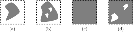
Figure 6: Admissible domains for the existence of weak solutions: (a) a simply connected bounded domain; (b) a bounded domain with holes; (c) the whole plane; (d) an exterior domain.

Definition 2.10 (admissible boundary condition).

If $\Omega$ is an admissible domain, an admissible boundary condition is a field $\boldsymbol{u}^{*}\in W^{1/2,2}(\partial\Omega)$, defined on the boundary such that if $\Omega$ is bounded, the total flux is zero,

$$\int_{\partial\Omega}\boldsymbol{u}^{*}\boldsymbol{\cdot}\boldsymbol{n}=0\,.$$

We define the flux through each bounded component $B_{i}$ by

$$\Phi_{i}=\int_{\partial B_{i}}\boldsymbol{u}^{*}\boldsymbol{\cdot}\boldsymbol{n}\,,$$

and we denote the sum of the magnitude of the fluxes by $\Phi$,

$$\Phi=\sum_{i=1}^{k}\left|\Phi_{i}\right|\,.$$

Lemma 2.11.

If $\Omega$ is an admissible domain and $\boldsymbol{u}^{*}\in W^{1/2,2}(\partial\Omega)$ an admissible boundary condition, then there exists an extension $\boldsymbol{a}\in D_{\sigma}^{1,2}(\Omega)\cap L^{4}(\Omega)$ such that $\boldsymbol{u}^{*}=\boldsymbol{a}$ in the trace sense on $\partial\Omega$, and moreover, there exists a constant $C>0$ depending on the domain and on $\boldsymbol{u}^{*}$ such that

$$\bigl{|}\bigl{(}\boldsymbol{v}\boldsymbol{\cdot}\boldsymbol{\nabla}\boldsymbol{a},\boldsymbol{v}\bigr{)}\bigr{|}\leq\left(\frac{1}{4}+C\Phi\right)\left\|\boldsymbol{\nabla}\boldsymbol{v}\right\|_{2}^{2}$$

for all $\boldsymbol{v}\in D_{0,\sigma}^{1,2}(\Omega)$.

Proof.

For each $i=1,\dots,k$, there exists $\boldsymbol{x}_{i}\in B_{i}$. We consider the field $\boldsymbol{a}_{\Phi}\in C_{\sigma}^{\infty}(\macc@depth\char 1\relax\frozen@everymath{\macc@group}\macc@set@skewchar\macc@nested@a 111{})$ defined by

$$\boldsymbol{a}_{\Phi}(\boldsymbol{x})=\frac{1}{2\pi\left(n-1\right)}\sum_{i=1}^{k}\Phi_{i}\frac{\boldsymbol{x}-\boldsymbol{x}_{i}}{\left|\boldsymbol{x}-\boldsymbol{x}_{i}\right|^{n}}\,.$$

By construction, the boundary field $\boldsymbol{u}^{*}-\boldsymbol{a}_{\Phi}$ has zero flux through each connected component of $\partial\Omega$. Since the connected components of the boundary $\partial\Omega$ are separated, by using extension-basic, there exists $\delta>0$ and an extension $\boldsymbol{a}_{\delta}\in W_{\sigma}^{1,2}(\Omega)\cap L^{4}(\Omega)$ of $\boldsymbol{u}^{*}-\boldsymbol{a}_{\Phi}$ such that

$$\bigl{|}\bigl{(}\boldsymbol{v}\boldsymbol{\cdot}\boldsymbol{\nabla}\boldsymbol{a}_{\delta},\boldsymbol{v}\bigr{)}\bigr{|}\leq\frac{1}{4}\left\|\boldsymbol{\nabla}\boldsymbol{v}\right\|_{2}^{2}\,.$$

By integrating by parts and using that $\boldsymbol{v}$ is divergence free, we have

$$\bigl{(}\boldsymbol{v}\boldsymbol{\cdot}\boldsymbol{\nabla}\boldsymbol{a}_{\Phi},\boldsymbol{v}\bigr{)}=-\bigl{(}\boldsymbol{v}\boldsymbol{\cdot}\boldsymbol{\nabla}\boldsymbol{v},\boldsymbol{a}_{\Phi}\bigr{)}=\int_{\Omega}\boldsymbol{\nabla}\boldsymbol{\cdot}\left(\boldsymbol{v}\boldsymbol{\cdot}\boldsymbol{\nabla}\boldsymbol{v}\right)A_{\Phi}\,,$$

where $A_{\Phi}$ is the potential of $\boldsymbol{a}_{\Phi}$, i.e. $\boldsymbol{a}_{\Phi}=\boldsymbol{\nabla}A_{\Phi}$. We note that in case $\Omega$ is bounded, we could easily conclude the proof now, but not in the unbounded case. For $n=3$, we have

$$\left|\int_{\Omega}\boldsymbol{\nabla}\boldsymbol{\cdot}\left(\boldsymbol{v}\boldsymbol{\cdot}\boldsymbol{\nabla}\boldsymbol{v}\right)A_{\Phi}\right|\leq\int_{\Omega}\left|\boldsymbol{\nabla}\boldsymbol{v}\right|^{2}\left|A_{\Phi}\right|\leq\frac{1}{4\pi}\sum_{i=1}^{k}\left|\Phi_{i}\right|\sup_{x\in\Omega}\frac{1}{\left|\boldsymbol{x}-\boldsymbol{x}_{i}\right|}\left\|\boldsymbol{\nabla}\boldsymbol{v}\right\|_{2}^{2}\leq C\sum_{i=1}^{k}\left|\Phi_{i}\right|\left\|\boldsymbol{\nabla}\boldsymbol{v}\right\|_{2}^{2}\,,$$

where $C>0$ is a constant depending on the domain. For $n=2$, by using Coifman et al. (1993, Theorem II.1), $\boldsymbol{\nabla}\boldsymbol{\cdot}\left(\boldsymbol{v}\boldsymbol{\cdot}\boldsymbol{\nabla}\boldsymbol{v}\right)=\boldsymbol{\nabla}\boldsymbol{v}:\left(\boldsymbol{\nabla}\boldsymbol{v}\right)^{T}$ is in the Hardy space $\mathcal{H}^{1}$ and by using Taylor (2011, Proposition 12.11), we obtain that the form $\left(\boldsymbol{\nabla}\boldsymbol{\cdot}\left(\boldsymbol{v}\boldsymbol{\cdot}\boldsymbol{\nabla}\boldsymbol{v}\right),A_{\Phi}\right)$ is bilinear and continuous for $\boldsymbol{v}\in D_{\sigma}^{1,2}$, so there exists a constant $C>0$ depending on the domain such that

$$\left|\int_{\Omega}\boldsymbol{\nabla}\boldsymbol{\cdot}\left(\boldsymbol{v}\boldsymbol{\cdot}\boldsymbol{\nabla}\boldsymbol{v}\right)A_{\Phi}\right|\leq C\sum_{i=1}^{k}\left|\Phi_{i}\right|\left\|\boldsymbol{\nabla}\boldsymbol{v}\right\|_{2}^{2}\,.$$

Therefore, by choosing $\delta$ small enough, $\boldsymbol{a}=\boldsymbol{a}_{\Phi}+\boldsymbol{a}_{\delta}$ satisfies the statement of the lemma.∎

Lemma 2.12.

Let $B$ be a bounded and simply connected domain with smooth boundary. Let $\Omega$ be either $B$ or its complement $\mathbb{R}^{2}\setminus\macc@depth\char 1\relax\frozen@everymath{\macc@group}\macc@set@skewchar\macc@nested@a 111{B}$. If $\boldsymbol{u}^{*}\in W^{1/2,2}(\partial\Omega)$ is an admissible boundary condition with $\Phi=0$, then for all $\delta>0$, there exists an extension $\boldsymbol{a}_{\delta}\in W_{\sigma}^{1,2}(\Omega)\cap L^{4}(\Omega)$ of $\boldsymbol{u}^{*}$ having support in a tube of weight $\delta$ around the boundary, i.e. in $\left\{\boldsymbol{x}\in\Omega\,:\,\operatorname{dist}(\boldsymbol{x},\partial\Omega)\leq 2\delta\right\}$, and such that

$$\left|\left(\boldsymbol{v}\boldsymbol{\cdot}\boldsymbol{\nabla}\boldsymbol{a}_{\delta},\boldsymbol{v}\right)\right|\leq\frac{C}{\left|\log\delta\right|}\left\|\boldsymbol{\nabla}\boldsymbol{v}\right\|_{2}^{2}$$

for all $\boldsymbol{v}\in D_{0,\sigma}^{1,2}(\Omega)$ where $C>0$ is a constant depending on the domain and on $\boldsymbol{u}^{*}$.

Proof.

We will construct an extension having support near the boundary of $\Omega$. If $\Omega$ is unbounded, we can truncate the domain to some large enough ball and therefore, without lost of generality, we consider that $\Omega$ is bounded. Since $\boldsymbol{u}^{*}\in W^{1/2,2}(\partial\Omega)$ has zero flux, there exists $\boldsymbol{\psi}\in W^{2,2}(\Omega)$ such that $\boldsymbol{u}^{*}=\boldsymbol{\nabla}\boldsymbol{\wedge}\boldsymbol{\psi}$ on $\partial\Omega$ in the trace sense (Galdi, 1991). By Stein (1970, Chapter VI, Theorem 2), there exists a function $\rho\in C^{\infty}(\Omega)$ and $\kappa>0$, such that

$$\frac{1}{\kappa}\rho(\boldsymbol{x}) \leq\operatorname{dist}(\boldsymbol{x},\partial\Omega)\leq\rho(\boldsymbol{x})\,, \left|\boldsymbol{\nabla}\rho(\boldsymbol{x})\right| \leq\kappa\,.$$

We define

$$\Omega_{\delta}=\left\{\boldsymbol{x}\in\Omega\,:\,\operatorname{dist}(\boldsymbol{x},\partial\Omega)\leq\delta\right\}.$$

Let $\chi_{\delta}\in C_{0}^{\infty}(\mathbb{R},[0,1])$ be a smooth function such that $\chi_{\delta}(r)=1$ if $r\leq\delta^{2}/2$ and $\chi_{\delta}(r)=0$ if $r\geq 2\delta$, and moreover $\left|\chi_{\delta}^{\prime}(r)\right|\leq r^{-1}\left|\log(\delta)\right|^{-1}$. We define $\xi_{\delta}=\chi_{\delta}\circ\rho$ so that $\xi_{\delta}\in C_{0}^{\infty}(\macc@depth\char 1\relax\frozen@everymath{\macc@group}\macc@set@skewchar\macc@nested@a 111{})$, $\psi_{\delta}(\boldsymbol{x})=1$ $\operatorname{dist}(\boldsymbol{x},\partial\Omega)\leq\frac{\delta^{2}}{2\kappa}$, and $\xi_{\delta}(\boldsymbol{x})=0$ if $\operatorname{dist}(\boldsymbol{x},\partial\Omega)\geq 2\delta$. Moreover,

$$\left|\boldsymbol{\nabla}\xi_{\delta}(\boldsymbol{x})\right|=\left|\chi_{\delta}^{\prime}(\rho(\boldsymbol{x}))\left|\boldsymbol{\nabla}\rho(\boldsymbol{x})\right|\right|\leq\frac{\kappa}{\rho(\boldsymbol{x})\left|\log(\delta)\right|}\,.$$

By setting $\boldsymbol{\psi}_{\delta}=\xi_{\delta}\boldsymbol{\psi}$, $\boldsymbol{a}_{\delta}=\boldsymbol{\nabla}\boldsymbol{\wedge}\boldsymbol{\psi}_{\delta}$ is an extension of $\boldsymbol{u}^{*}$, which has support in $\Omega_{\delta}=\left\{\boldsymbol{x}\in\Omega\,:\,\operatorname{dist}(\boldsymbol{x},\partial\Omega)\leq 2\delta\right\}$.

Since

$$\boldsymbol{a}_{\delta}=\xi_{\delta}\boldsymbol{\nabla}\boldsymbol{\wedge}\boldsymbol{\psi}+\boldsymbol{\nabla}\xi_{\delta}\boldsymbol{\wedge}\boldsymbol{\psi}\,,$$

we have

$$\left\|\left|\boldsymbol{v}\right|\left|\boldsymbol{a}_{\delta}\right|\right\|_{2} \leq\left\|\left|\boldsymbol{v}\right|\left|\xi_{\delta}\right|\left|\boldsymbol{\nabla}\boldsymbol{\psi}\right|\right\|_{2}+\left\|\left|\boldsymbol{v}\right|\left|\boldsymbol{\nabla}\xi_{\delta}\right|\left|\boldsymbol{\psi}\right|\right\|_{2}$$

$$\leq\bigl{\|}\boldsymbol{v};L^{4}(\Omega_{\delta})\bigr{\|}\left\|\boldsymbol{\nabla}\boldsymbol{\psi}\right\|_{4}+\frac{\kappa}{\left|\log\delta\right|}\left\|\left|\boldsymbol{v}/\rho\right|\left|\boldsymbol{\psi}\right|\right\|_{2}\,.$$

By using the Hölder inequality and Sobolev embeddings, we have

$$\bigl{\|}\boldsymbol{v};L^{4}(\Omega_{\delta})\bigr{\|}\left\|\boldsymbol{\nabla}\boldsymbol{\psi}\right\|_{4} \leq C_{1}\bigl{\|}1;L^{12}(\Omega_{\delta})\bigr{\|}\bigl{\|}\boldsymbol{v};L^{6}(\Omega_{\delta})\bigr{\|}\bigl{\|}\boldsymbol{\psi};W^{2,2}(\Omega)\bigr{\|}$$

$$\leq\frac{C_{2}}{\left|\log\delta\right|}\bigl{\|}\boldsymbol{\nabla}\boldsymbol{v}\bigr{\|}_{2}\bigl{\|}\boldsymbol{\psi};W^{2,2}(\Omega)\bigr{\|}\,,$$

and by Hardy inequality,

$$\left\|\left|\boldsymbol{v}/\rho\right|\left|\boldsymbol{\psi}\right|\right\|_{2}\leq C_{3}\left\|\boldsymbol{\nabla}\boldsymbol{v}\right\|_{2}\left\|\boldsymbol{\psi}\right\|_{\infty}\leq C_{4}\left\|\boldsymbol{\nabla}\boldsymbol{v}\right\|_{2}\bigl{\|}\boldsymbol{\psi};W^{2,2}(\Omega)\bigr{\|}\,,$$

where $C_{i}$ are constants depending only on the domain $\Omega$. Therefore, there exists a constant $C>0$ depending on the domain $\Omega$ such that

$$\left\|\left|\boldsymbol{v}\right||\boldsymbol{a}_{\delta}|\right\|_{2}\leq\frac{C}{\left|\log\delta\right|}\left\|\boldsymbol{\nabla}\boldsymbol{v}\right\|_{2}\bigl{\|}\boldsymbol{\psi};W^{2,2}(\Omega)\bigr{\|}\,,$$

and finally by integrating by parts, we obtain the claimed bound

$$\bigl{|}\bigl{(}\boldsymbol{v}\boldsymbol{\cdot}\boldsymbol{\nabla}\boldsymbol{a}_{\delta},\boldsymbol{v}\bigr{)}\bigr{|}\leq\bigl{|}\bigl{(}\boldsymbol{v}\boldsymbol{\cdot}\boldsymbol{\nabla}\boldsymbol{v},\boldsymbol{a}_{\delta}\bigr{)}\bigr{|}\leq\left\|\boldsymbol{\nabla}\boldsymbol{v}\right\|_{2}\left\|\left|\boldsymbol{v}\right||\boldsymbol{a}_{\delta}|\right\|_{2}\leq\frac{C\bigl{\|}\boldsymbol{\psi};W^{2,2}(\Omega)\bigr{\|}}{\left|\log\delta\right|}\left\|\boldsymbol{\nabla}\boldsymbol{v}\right\|_{2}^{2}\,.$$

∎

6 Existence of weak solutions

Definition 2.13.

A vector field $\boldsymbol{u}:\Omega\to\mathbb{R}^{n}$ is called a weak solution to (LABEL:intro-ns) if

1. $\boldsymbol{u}\in D_{\sigma}^{1,2}(\Omega)$;

2. $\left.\boldsymbol{u}\right|_{\partial\Omega}=\boldsymbol{u}^{*}$ in the trace sense;

3. $\boldsymbol{u}$ satisfies

   $$\bigl{(}\boldsymbol{\nabla}\boldsymbol{u},\boldsymbol{\nabla}\boldsymbol{\varphi}\bigr{)}+\bigl{(}\boldsymbol{u}\boldsymbol{\cdot}\boldsymbol{\nabla}\boldsymbol{u},\boldsymbol{\varphi}\bigr{)}+\bigl{(}\boldsymbol{f},\boldsymbol{\varphi}\bigr{)}=0$$ (13)

   for all $\boldsymbol{\varphi}\in C_{0,\sigma}^{\infty}(\Omega)$.

Remark 2.14.

We note that in this definition, there is no mention of the limit of $\boldsymbol{u}$ at infinity in case $\Omega$ is unbounded. The limit of $\boldsymbol{u}$ at infinity will be discussed in weal-solution-limit.

If the total $\Phi$ is small enough, there exists a weak solution as stated by:

Theorem 2.15.

If $\Omega\neq\mathbb{R}^{2}$ is an admissible domain, $\boldsymbol{u}^{*}\in W^{1/2,2}(\partial\Omega)$ an admissible boundary condition with $\Phi$ small enough, there exists a weak solution to (LABEL:intro-ns), provided $\left(\boldsymbol{f},\boldsymbol{\varphi}\right)$ defines a linear functional on $\boldsymbol{\varphi}\in D_{0,\sigma}^{1,2}(\Omega)$.

Remark 2.16.

In symmetric unbounded domains, Korobkov et al. (2014a, b) showed the existence of a weak solution for arbitrary large $\Phi$. This was recently improved by Korobkov et al. (2015) that showed the existence of weak solutions in two-dimensional bounded domains without any symmetry and smallness assumptions.

Remark 2.17.

Ladyzhenskaya (1969, pp. 36–37) listed some conditions on $\boldsymbol{f}$, so that $\left(\boldsymbol{f},\boldsymbol{\varphi}\right)$ defines a linear functional on $\boldsymbol{\varphi}\in D_{0,\sigma}^{1,2}(\Omega)$.

Proof.

We treat the case where $\Omega$ is bounded and unbounded in parallel. In case $\Omega$ is bounded, we set $\boldsymbol{u}_{\infty}=\boldsymbol{0}$ by convenience in what follows. By using Riesz’ theorem, there exists $\boldsymbol{F}\in D_{0,\sigma}^{1,2}(\Omega)$, such that

$$\bigl{[}\boldsymbol{F},\boldsymbol{\varphi}\bigr{]}=\bigl{(}\boldsymbol{f},\boldsymbol{\varphi}\bigr{)}\,,$$

where $\left[\cdot,\cdot\right]$ denotes the scalar product in $D_{0,\sigma}^{1,2}(\Omega)$. We look for a solution of the form $\boldsymbol{u}=\boldsymbol{u}_{\infty}+\boldsymbol{a}+\boldsymbol{v}$, where $\boldsymbol{a}$ is the extension of $\boldsymbol{u}^{*}-\boldsymbol{u}_{\infty}$ given by extention, so that $\boldsymbol{v}$ vanishes at the boundary and with the hope that $\boldsymbol{v}$ will converges to zero for large $\boldsymbol{x}$ in case $\Omega$ is unbounded.

1. We first treat the case where $\Omega$ is bounded, so that $D_{0,\sigma}^{1,2}(\Omega)=W_{0,\sigma}^{1,2}(\Omega)$, and $D_{0,\sigma}^{1,2}(\Omega)$ is compactly embedded in $L^{4}(\Omega)$. First of all, by integrating by parts we have since $\boldsymbol{u}$ is divergence-free,

   $$\bigl{(}\boldsymbol{u}\boldsymbol{\cdot}\boldsymbol{\nabla}\boldsymbol{u},\boldsymbol{\varphi}\bigr{)}+\bigl{(}\boldsymbol{u}\boldsymbol{\cdot}\boldsymbol{\nabla}\boldsymbol{\varphi},\boldsymbol{u}\bigr{)}=\int_{\Omega}\boldsymbol{\nabla}\boldsymbol{\cdot}\left(\boldsymbol{u}\boldsymbol{\cdot}\boldsymbol{\varphi}\,\boldsymbol{u}\right)=\int_{\partial\Omega}\boldsymbol{u}\boldsymbol{\cdot}\boldsymbol{\varphi}\,\boldsymbol{u}\boldsymbol{\cdot}\boldsymbol{n}=0\,.$$

   By the Riesz’ theorem there exists $\boldsymbol{B}\in D_{0,\sigma}^{1,2}(\Omega)$ such that

   $$\bigl{[}\boldsymbol{B},\boldsymbol{\varphi}\bigr{]}=\bigl{(}\boldsymbol{\nabla}\boldsymbol{a},\boldsymbol{\nabla}\boldsymbol{\varphi}\bigr{)}+\bigl{(}\boldsymbol{a}\boldsymbol{\cdot}\boldsymbol{\nabla}\boldsymbol{a},\boldsymbol{\varphi}\bigr{)}\,,$$

   because

   $$\bigl{|}\bigl{[}\boldsymbol{B},\boldsymbol{\varphi}\bigr{]}\bigr{|}\leq\bigl{|}\bigl{(}\boldsymbol{\nabla}\boldsymbol{a},\boldsymbol{\nabla}\boldsymbol{\varphi}\bigr{)}\bigr{|}+\bigl{|}\bigl{(}\boldsymbol{a}\boldsymbol{\cdot}\boldsymbol{\nabla}\boldsymbol{\varphi},\boldsymbol{a}\bigr{)}\bigr{|}\leq\left\|\boldsymbol{\nabla}\boldsymbol{a}\right\|_{2}\left\|\boldsymbol{\nabla}\boldsymbol{\varphi}\right\|_{2}+\left\|\boldsymbol{a}\right\|_{4}^{2}\left\|\boldsymbol{\nabla}\boldsymbol{\varphi}\right\|_{2}\,.$$

   In the same way, there exists a map $A:D_{0,\sigma}^{1,2}(\Omega)\to D_{0,\sigma}^{1,2}(\Omega)$ such that

   $$\bigl{[}A\boldsymbol{v},\boldsymbol{\varphi}\bigr{]}=\bigl{(}\boldsymbol{a}\boldsymbol{\cdot}\boldsymbol{\nabla}\boldsymbol{v},\boldsymbol{\varphi}\bigr{)}+\bigl{(}\boldsymbol{v}\boldsymbol{\cdot}\boldsymbol{\nabla}\boldsymbol{a},\boldsymbol{\varphi}\bigr{)}+\bigl{(}\boldsymbol{v}\boldsymbol{\cdot}\boldsymbol{\nabla}\boldsymbol{v},\boldsymbol{\varphi}\bigr{)}\,,$$

   because

   $$\bigl{|}\bigl{[}A\boldsymbol{v},\boldsymbol{\varphi}\bigr{]}\bigr{|}\leq\bigl{|}\bigl{(}\boldsymbol{a}\boldsymbol{\cdot}\boldsymbol{\nabla}\boldsymbol{\varphi},\boldsymbol{v}\bigr{)}\bigr{|}+\bigl{|}\bigl{(}\boldsymbol{v}\boldsymbol{\cdot}\boldsymbol{\nabla}\boldsymbol{\varphi},\boldsymbol{a}\bigr{)}\bigr{|}+\bigl{|}\bigl{(}\boldsymbol{v}\boldsymbol{\cdot}\boldsymbol{\nabla}\boldsymbol{\varphi},\boldsymbol{v}\bigr{)}\bigr{|}\leq\left(2\left\|\boldsymbol{a}\right\|_{4}+\left\|\boldsymbol{v}\right\|_{4}\right)\left\|\boldsymbol{\nabla}\boldsymbol{\varphi}\right\|_{2}\left\|\boldsymbol{v}\right\|_{4}$$

   Since $D_{0,\sigma}^{1,2}(\Omega)$ is compactly embedded in $L^{4}(\Omega)$, the map $A$ is continuous on $D_{0,\sigma}^{1,2}(\Omega)$ when equipped with the $L^{4}$-norm and therefore is completely continuous on $D_{0,\sigma}^{1,2}(\Omega)$ when equipped with its underlying norm.

   The condition (LABEL:weak-solution-short) is equivalent to

   $$\bigl{[}\boldsymbol{v}+A\boldsymbol{v}+\boldsymbol{B}+\boldsymbol{F},\boldsymbol{\varphi}\bigr{]}=0\,,$$

   which corresponds to solving the nonlinear equation

   $$\boldsymbol{v}+A\boldsymbol{v}+\boldsymbol{B}+\boldsymbol{F}=0$$ (14)

   in $D_{0,\sigma}^{1,2}(\Omega)$. From the Leray-Schauder fixed point theorem (see for example Gilbarg & Trudinger, 1998, Theorem 11.6) to prove the existence of a solution to (LABEL:ns-functional) it is sufficient to prove that the set of solutions $\boldsymbol{v}$ of the equation

   $$\boldsymbol{v}+\lambda\left(A\boldsymbol{v}+\boldsymbol{B}+\boldsymbol{F}\right)=0$$ (15)

   is uniformly bounded in $\lambda\in\left[0,1\right]$. To this end, we take the scalar product of (LABEL:ns-functional-lambda) with $\boldsymbol{v}$,

   $$\bigl{(}\boldsymbol{\nabla}\boldsymbol{v},\boldsymbol{\nabla}\boldsymbol{v}\bigr{)}+\lambda\bigl{(}\boldsymbol{v}\boldsymbol{\cdot}\boldsymbol{\nabla}\boldsymbol{a},\boldsymbol{v}\bigr{)}+\lambda\bigl{(}\boldsymbol{u}\boldsymbol{\cdot}\boldsymbol{\nabla}\boldsymbol{v},\boldsymbol{v}\bigr{)}+\lambda\bigl{(}\boldsymbol{\nabla}\boldsymbol{a},\boldsymbol{\nabla}\boldsymbol{v}\bigr{)}+\lambda\bigl{(}\boldsymbol{a}\boldsymbol{\cdot}\boldsymbol{\nabla}\boldsymbol{a},\boldsymbol{v}\bigr{)}+\lambda\bigl{(}\boldsymbol{f},\boldsymbol{v}\bigr{)}=0\,.$$

   where $\boldsymbol{u}=\boldsymbol{a}+\boldsymbol{v}$. We have

   $$\bigl{(}\boldsymbol{u}\boldsymbol{\cdot}\boldsymbol{\nabla}\boldsymbol{v},\boldsymbol{v}\bigr{)}=\frac{1}{2}\int_{\Omega}\boldsymbol{\nabla}\boldsymbol{\cdot}\left(\boldsymbol{v}\boldsymbol{\cdot}\boldsymbol{v}\,\boldsymbol{u}\right)=\frac{1}{2}\int_{\partial\Omega}\left(\boldsymbol{v}\boldsymbol{\cdot}\boldsymbol{v}\,\boldsymbol{u}\boldsymbol{\cdot}\boldsymbol{n}\right)=0\,,$$

   and by extention, if $\Phi$ is small enough,

   $$\bigl{|}\bigl{(}\boldsymbol{v}\boldsymbol{\cdot}\boldsymbol{\nabla}\boldsymbol{a},\boldsymbol{v}\bigr{)}\bigr{|}\leq\frac{1}{2}\left\|\boldsymbol{\nabla}\boldsymbol{v}\right\|_{2}^{2}\,,$$

   so by Hölder inequality, we obtain

   $$\left\|\boldsymbol{\nabla}\boldsymbol{v}\right\|_{2}^{2} \leq\frac{1}{2}\left\|\boldsymbol{\nabla}\boldsymbol{v}\right\|_{2}^{2}+\left\|\boldsymbol{\nabla}\boldsymbol{a}\right\|_{2}\left\|\boldsymbol{\nabla}\boldsymbol{v}\right\|_{2}+\left\|\boldsymbol{a}\right\|_{4}^{2}\left\|\boldsymbol{\nabla}\boldsymbol{v}\right\|_{2}+\left\|\boldsymbol{\nabla}\boldsymbol{F}\right\|_{2}\left\|\boldsymbol{\nabla}\boldsymbol{v}\right\|_{2}$$

   $$\leq\frac{1}{2}\left\|\boldsymbol{\nabla}\boldsymbol{v}\right\|_{2}^{2}+\left(\left\|\boldsymbol{\nabla}\boldsymbol{a}\right\|_{2}+\left\|\boldsymbol{a}\right\|_{4}^{2}\right)\left\|\boldsymbol{\nabla}\boldsymbol{v}\right\|_{2}+\left\|\boldsymbol{\nabla}\boldsymbol{F}\right\|_{2}\left\|\boldsymbol{\nabla}\boldsymbol{v}\right\|_{2}\,.$$

   Consequently, we have

   $$\left\|\boldsymbol{\nabla}\boldsymbol{v}\right\|_{2}\leq\frac{\left\|\boldsymbol{\nabla}\boldsymbol{a}\right\|_{2}+\left\|\boldsymbol{a}\right\|_{4}^{2}+\left\|\boldsymbol{\nabla}\boldsymbol{F}\right\|_{2}}{2}\,.$$

2. We now consider the case where $\Omega$ is unbounded. There exists $R>0$ such that $\mathbb{R}^{n}\setminus\Omega$ is contained in $B(\boldsymbol{0},R)$. For $n\in\mathbb{N}$, we consider the domains $\Omega_{n}=\Omega\cap B(\boldsymbol{0},R+n)$. By the existence result for the bounded case, there exists for each $n\in\mathbb{N}$ a weak solution $\boldsymbol{u}_{n}=\boldsymbol{u}_{\infty}+\boldsymbol{a}+\boldsymbol{v}_{n}$, where $\boldsymbol{v}_{n}\in D_{0,\sigma}^{1,2}(\Omega_{n})$ to (LABEL:intro-ns-eq) in $\Omega_{n}$, with $\boldsymbol{u}^{*}=\boldsymbol{u}_{\infty}+\boldsymbol{a}$ on $\partial\Omega_{n}$. By extending $\boldsymbol{v}_{n}$ to $\Omega$ by setting $\boldsymbol{v}_{n}=\boldsymbol{0}$ on $\Omega\setminus\Omega_{n}$, then $\boldsymbol{v}_{n}\in D_{0,\sigma}^{1,2}(\Omega)$ and the sequence $\left(\boldsymbol{v}_{n}\right)_{n\in\mathbb{N}}$ is bounded in $D_{0,\sigma}^{1,2}(\Omega)$. Therefore, there exists a subsequence, denoted also by $\left(\boldsymbol{v}_{n}\right)_{n\in\mathbb{N}}$, which converges weakly to some $\boldsymbol{v}$ in $D_{0,\sigma}^{1,2}(\Omega)$. We now show that $\boldsymbol{u}=\boldsymbol{u}_{\infty}+\boldsymbol{a}+\boldsymbol{v}$ is a weak solution to (LABEL:intro-ns) in $\Omega$. Given $\boldsymbol{\varphi}\in C_{0,\sigma}^{\infty}(\Omega)$, there exists $m\in\mathbb{N}$ such that the support of $\boldsymbol{\varphi}$ is contained in $\Omega_{m}$. Therefore, for any $n\geq m$, we have

   $$\bigl{(}\boldsymbol{\nabla}\boldsymbol{u}_{n},\boldsymbol{\nabla}\boldsymbol{\varphi}\bigr{)}+\bigl{(}\boldsymbol{u}_{n}\boldsymbol{\cdot}\boldsymbol{\nabla}\boldsymbol{u}_{n},\boldsymbol{\varphi}\bigr{)}+\bigl{(}\boldsymbol{f},\varphi\bigr{)}=0\,,$$

   and it only remains to show that the equation is valid in the limit $n\to\infty$. By definition of the weak convergence,

   $$\lim_{n\to\infty}\bigl{(}\boldsymbol{\nabla}\boldsymbol{v}_{n},\boldsymbol{\nabla}\boldsymbol{\varphi}\bigr{)}=\bigl{(}\boldsymbol{\nabla}\boldsymbol{v},\boldsymbol{\nabla}\boldsymbol{\varphi}\bigr{)}\,,$$

   and since $\boldsymbol{\varphi}$ has compact support in $\Omega_{m}$,

   $$\bigl{|}\bigl{(}\boldsymbol{u}_{n}\boldsymbol{\cdot}\boldsymbol{\nabla}\boldsymbol{u}_{n}-\boldsymbol{u}\boldsymbol{\cdot}\boldsymbol{\nabla}\boldsymbol{u},\boldsymbol{\varphi}\bigr{)}\bigr{|} \leq\bigl{|}\left(\left(\boldsymbol{u}_{n}-\boldsymbol{u}\right)\boldsymbol{\cdot}\boldsymbol{\nabla}\boldsymbol{u}_{n},\boldsymbol{\varphi}\right)\bigr{|}+\bigl{|}\left(\boldsymbol{u}\boldsymbol{\cdot}\left(\boldsymbol{\nabla}\boldsymbol{u}_{n}-\boldsymbol{\nabla}\boldsymbol{u}\right),\boldsymbol{\varphi}\right)\bigr{|}$$

   $$\leq\bigl{|}\left(\left(\boldsymbol{u}_{n}-\boldsymbol{u}\right)\boldsymbol{\cdot}\boldsymbol{\nabla}\boldsymbol{u}_{n},\boldsymbol{\varphi}\right)\bigr{|}+\bigl{|}\left(\boldsymbol{u}\boldsymbol{\cdot}\boldsymbol{\nabla}\boldsymbol{\varphi},\boldsymbol{v}_{n}-\boldsymbol{v}\right)\bigr{|}$$

   $$\leq\bigl{|}\left(\left(\boldsymbol{v}_{n}-\boldsymbol{v}\right)\boldsymbol{\cdot}\boldsymbol{\nabla}\boldsymbol{u}_{n},\boldsymbol{\varphi}\right)\bigr{|}+\bigl{|}\left(\boldsymbol{u}\boldsymbol{\cdot}\boldsymbol{\nabla}\boldsymbol{\varphi},\boldsymbol{v}_{n}-\boldsymbol{v}\right)\bigr{|}$$

   $$\leq\left(\left\|\boldsymbol{\nabla}\boldsymbol{u}_{n}\right\|_{2}\left\|\boldsymbol{\varphi}\right\|_{4}+\bigl{\|}\boldsymbol{u};L^{4}(\Omega_{m})\bigr{\|}\left\|\boldsymbol{\nabla}\boldsymbol{\varphi}\right\|_{2}\right)\bigl{\|}\boldsymbol{v}_{n}-\boldsymbol{v};L^{4}(\Omega_{m})\bigr{\|}\,.$$

   By local-D0, the sequence $\left(\boldsymbol{v}_{n}\right)_{n\in\mathbb{N}}$ is bounded in $W^{1,2}(\Omega_{m})$ and by compact-embedding, there exists a subsequence also denoted by $\left(\boldsymbol{v}_{n}\right)_{n\in\mathbb{N}}$ which converges strongly to $\boldsymbol{v}$ in $L^{4}(\Omega_{m})$. Therefore,

   $$\lim_{n\to\infty}\bigl{(}\boldsymbol{u}_{n}\boldsymbol{\cdot}\boldsymbol{\nabla}\boldsymbol{u}_{n},\boldsymbol{\varphi}\bigr{)}=\bigl{(}\boldsymbol{u}\boldsymbol{\cdot}\boldsymbol{\nabla}\boldsymbol{u},\boldsymbol{\varphi}\bigr{)}\,.$$

   and $\boldsymbol{u}$ satisfies (LABEL:weak-solution-short).

∎

7 Regularity of weak solutions

A weak solution is a vector field $\boldsymbol{u}\in D_{\sigma}^{1,2}(\Omega)$ that satisfies the Navier-Stokes equations in a variational way and therefore a weak solution is defined even for low regularity on the data $\boldsymbol{u}^{*}$ and $\boldsymbol{f}$ and does not necessarily satisfies the equations in a classical way. By assuming more regularity on the data, any weak solution becomes more regular and satisfies the Navier-Stokes equations in the classical way. The following theorem states this fact:

Theorem 2.18 (Galdi, 2011, Theorems IX.5.1, IX.5.2 and X.1.1).

Let $\boldsymbol{u}$ be a weak solution according to weak-solution. The following properties hold:

1. For $m\geq 1$ if $\boldsymbol{f}\in W_{loc}^{m,2}(\Omega)$, then $\boldsymbol{u}\in W_{loc}^{m+2,2}(\Omega)$ and $p\in W_{loc}^{m+1,2}(\Omega)$.

2. If $\Omega$ is a smooth domain, $\boldsymbol{u}^{*}\in C^{\infty}(\partial\Omega)$ and $\boldsymbol{f}\in C^{\infty}(\macc@depth\char 1\relax\frozen@everymath{\macc@group}\macc@set@skewchar\macc@nested@a 111{})$, then $\boldsymbol{u},p\in C^{\infty}(\macc@depth\char 1\relax\frozen@everymath{\macc@group}\macc@set@skewchar\macc@nested@a 111{})$.

8 Limit of the velocity at large distances

We start with two lemmas (Ladyzhenskaya, 1969, §1.4) on the behavior at infinity of functions in $D_{0}^{1,2}(\Omega)$, with $\Omega$ unbounded. Due to the presence of a logarithm if $n=2$, the discussion of the validity of

$$\lim_{\left|\boldsymbol{x}\right|\to\infty}\boldsymbol{u}=\boldsymbol{u}_{\infty}\,,$$ (16)

for a weak solution depends drastically on the dimension.

Lemma 2.19 (Galdi, 2011, Theorem II.6.1).

For $n\geq 3$, if $\Omega\subset\mathbb{R}^{n}$ is an unbounded Lipschitz domain, then for all $\boldsymbol{u}\in D_{0}^{1,2}(\Omega)$,

$$\left\|\frac{\boldsymbol{u}}{\left|\boldsymbol{x}\right|}\right\|_{2}\leq\frac{2}{n-2}\left\|\boldsymbol{\nabla}\boldsymbol{u}\right\|_{2}\,.$$

Proof.

It suffices to prove the inequality for a scalar field $u\in C_{0}^{\infty}(\mathbb{R}^{n})$. Since

$$\boldsymbol{\nabla}\boldsymbol{\cdot}\left(\frac{\boldsymbol{x}}{\left|\boldsymbol{x}\right|^{2}}\right)=\frac{n-2}{\left|\boldsymbol{x}\right|^{2}}\,,$$

we have by integrating by parts,

$$\int_{\mathbb{R}^{n}}\frac{u^{2}}{\left|\boldsymbol{x}\right|^{2}}=-\frac{1}{n-2}\int_{\mathbb{R}^{n}}\frac{\boldsymbol{x}}{\left|\boldsymbol{x}\right|^{2}}\boldsymbol{\cdot}\boldsymbol{\nabla}\left(u^{2}\right)=-\frac{2}{n-2}\int_{\mathbb{R}^{n}}\frac{\boldsymbol{x}}{\left|\boldsymbol{x}\right|^{2}}\boldsymbol{\cdot}\boldsymbol{\nabla}u\,u\,.$$

Then by Schwarz inequality, we obtain

$$\left\|\frac{u}{\left|\boldsymbol{x}\right|}\right\|_{2}^{2}\leq\frac{2}{n-2}\left\|\frac{\boldsymbol{x}}{\left|\boldsymbol{x}\right|^{2}}u\right\|_{2}\left\|\boldsymbol{\nabla}u\right\|_{2}\leq\frac{2}{n-2}\left\|\frac{u}{\left|\boldsymbol{x}\right|}\right\|_{2}\left\|\boldsymbol{\nabla}u\right\|_{2}\,,$$

and the inequality is proved.∎

Lemma 2.20 (Galdi, 2011, Theorem II.6.1).

If $\Omega\subset\mathbb{R}^{2}$ is an exterior Lipschitz domain such that $B(\boldsymbol{0},\varepsilon)\subset\mathbb{R}^{2}\setminus\Omega$ for some $\varepsilon>0$, then for all $\boldsymbol{u}\in D_{0}^{1,2}(\Omega)$,

$$\left\|\frac{\boldsymbol{u}}{\left|\boldsymbol{x}\right|\log(\left|\boldsymbol{x}\right|/\varepsilon)}\right\|_{2}\leq 2\left\|\boldsymbol{\nabla}\boldsymbol{u}\right\|_{2}\,.$$

Proof.

Again, it is sufficient to prove the inequality for the scalar field $u\in C_{0}^{\infty}(\mathbb{R}^{2}\setminus\macc@depth\char 1\relax\frozen@everymath{\macc@group}\macc@set@skewchar\macc@nested@a 111{B}(\boldsymbol{0},\varepsilon))$. Since

$$\boldsymbol{\nabla}\boldsymbol{\cdot}\left(\frac{\boldsymbol{x}}{\left|\boldsymbol{x}\right|^{2}\log(\left|\boldsymbol{x}\right|/\varepsilon)}\right)=-\frac{1}{\left|\boldsymbol{x}\right|^{2}\log^{2}(\left|\boldsymbol{x}\right|/\varepsilon)}\,,$$

by integrating by parts,

$$\int_{\mathbb{R}^{2}}\frac{u^{2}}{\left|\boldsymbol{x}\right|^{2}\log^{2}(\left|\boldsymbol{x}\right|/\varepsilon)}=\int_{\mathbb{R}^{2}}\frac{\boldsymbol{x}}{\left|\boldsymbol{x}\right|^{2}\log(\left|\boldsymbol{x}\right|/\varepsilon)}\boldsymbol{\cdot}\boldsymbol{\nabla}\left(u^{2}\right)=\int_{\mathbb{R}^{2}}\frac{\boldsymbol{x}}{\left|\boldsymbol{x}\right|^{2}\log(\left|\boldsymbol{x}\right|/\varepsilon)}\boldsymbol{\cdot}\boldsymbol{\nabla}u\,u\,.$$

Then the lemma is proven by using the Schwartz inequality,

$$\left\|\frac{u}{\left|\boldsymbol{x}\right|\log(\left|\boldsymbol{x}\right|/\varepsilon)}\right\|_{2}^{2}\leq 2\left\|\frac{\boldsymbol{x}}{\left|\boldsymbol{x}\right|^{2}\log(\left|\boldsymbol{x}\right|/\varepsilon)}u\right\|_{2}\left\|\boldsymbol{\nabla}u\right\|_{2}\leq 2\left\|\frac{u}{\left|\boldsymbol{x}\right|\log(\left|\boldsymbol{x}\right|/\varepsilon)}\right\|_{2}\left\|\boldsymbol{\nabla}u\right\|_{2}\,.$$

∎

8.1 Three dimensions

By using hardy-3d, we can now prove that a function in $D_{0}^{1,2}(\Omega)$ tends to zero at infinity. In what follows, we set $B_{r}=B(\boldsymbol{0},r)$.

Lemma 2.21.

For $n=3$, if $\boldsymbol{u}\in D_{0}^{1,2}(\Omega)$, then

$$\int_{S^{2}}\left|\boldsymbol{u}\right|^{2}=O(\left|\boldsymbol{x}\right|^{-1})\,,$$

where $S^{2}\subset\mathbb{R}^{3}$ is the sphere of unit radius, or more precisely

$$\frac{1}{\left|\partial B_{r}\right|}\int_{\partial B_{r}}\left|\boldsymbol{u}\right|^{2}=O(r^{-1})\,.$$

Proof.

There exists $R>0$ such that $\mathbb{R}^{3}\setminus\Omega\subset B_{R}$. For $r\geq 1$. By the trace theorem in $B_{R}$, there exists $C>0$ such that for all $\boldsymbol{u}\in W^{1,2}(B_{R})$,

$$\bigl{\|}\boldsymbol{u};L^{2}(\partial B_{R})\bigr{\|}^{2}\leq C\left(\bigl{\|}\boldsymbol{u};L^{2}(B_{R})\bigr{\|}^{2}+\bigl{\|}\boldsymbol{\nabla}\boldsymbol{u};L^{2}(B_{R})\bigr{\|}^{2}\right)\,.$$

By a scaling argument, we have, for all $r\geq R$,

$$\frac{R^{2}}{r^{2}}\bigl{\|}\boldsymbol{u};L^{2}(\partial B_{r})\bigr{\|}^{2} \leq\frac{CR^{3}}{r^{3}}\bigl{\|}\boldsymbol{u};L^{2}(B_{r})\bigr{\|}^{2}+\frac{CR}{r}\bigl{\|}\boldsymbol{\nabla}\boldsymbol{u};L^{2}(B_{r})\bigr{\|}^{2}$$

$$\leq\frac{CR\left(1+R^{2}\right)}{r}\left[\bigl{\|}\boldsymbol{u}/\left|\boldsymbol{x}\right|;L^{2}(B_{r})\bigr{\|}^{2}+\bigl{\|}\boldsymbol{\nabla}\boldsymbol{u};L^{2}(B_{r})\bigr{\|}^{2}\right]\,.$$

By using hardy-3d, we have for some $C>0$ independent of $r$,

$$\frac{1}{r^{2}}\bigl{\|}\boldsymbol{u};L^{2}(\partial B_{r})\bigr{\|}^{2}\leq\frac{C}{r}\bigl{\|}\boldsymbol{\nabla}\boldsymbol{u};L^{2}(\Omega)\bigr{\|}^{2}\,.$$

Since $\left|\partial B_{r}\right|=4\pi r^{2}$, this completes the proof. ∎

By applying this lemma to the weak solution constructed in existence-weak, we obtain its behavior at infinity:

Proposition 2.22.

Let the hypothesis of existence-weak-solutions be satisfied, so that there exists a weak solution $\boldsymbol{u}\in D_{0,\sigma}^{1,2}$. In case $\Omega\subset\mathbb{R}^{3}$ is unbounded, we have (LABEL:weak-limit) in the following sense

$$\int_{S^{2}}\left|\boldsymbol{u}-\boldsymbol{u}_{\infty}\right|^{2}=O(\left|\boldsymbol{x}\right|^{-1})\,.$$

Proof.

The weak solution has the form $\boldsymbol{u}-\boldsymbol{u}_{\infty}=\boldsymbol{a}+\boldsymbol{v}$. By construction, $\boldsymbol{a}$ has one part of compact support, and one part carrying the fluxes decaying like $\left|\boldsymbol{x}\right|^{-2}$, so $\boldsymbol{a}=O(\left|\boldsymbol{x}\right|^{-2})$. By applying limit-3d to $\boldsymbol{v}\in D_{\sigma,0}^{1,2}(\Omega)$, we obtain the claimed result. ∎

8.2 Two dimensions

In two dimensions, the information contained in the space $D_{0}^{1,2}(\Omega)$ is not sufficient to determine the limit of the velocity at infinity, mainly due to the failure of hardy-3d for $n=2$. In fact a function in $D_{\sigma,0}^{1,2}(\Omega)$ can even grow at infinity, as shown by the following example. Therefore, the choice of $\boldsymbol{u}_{\infty}$ is apparently completely lost during the construction of weak solutions.

Example 2.23.

Let $\Omega\subset\mathbb{R}^{2}$ be an unbounded Lipschitz domain. For $R>0$ such that $\mathbb{R}^{2}\setminus\Omega\subset B(\boldsymbol{0},R)$, let $\chi$ be a cut-off function such that $\chi(\boldsymbol{x})=0$ for $\left|\boldsymbol{x}\right|\leq R$, and $\chi(\boldsymbol{x})=1$ for $\left|\boldsymbol{x}\right|\geq 2R$. For $\nu\in\bigl{[}\frac{-1}{2};\frac{1}{2}\bigr{)}$, the function $\boldsymbol{u}=\boldsymbol{\nabla}\boldsymbol{\wedge}\left(\chi\psi\right)$, where

$$\psi=-x_{2}\,\log^{\nu}\left|\boldsymbol{x}\right|\,,$$

satisfies $\boldsymbol{u}\in D_{0,\sigma}^{1,2}(\Omega)$, $\boldsymbol{u}/\left|\boldsymbol{x}\right|\notin L^{2}(\Omega)$ and $\boldsymbol{u}=O(\log^{\nu}\left|\boldsymbol{x}\right|)$ at infinity.

Proof.

By construction, $\boldsymbol{u}(\boldsymbol{x})=\boldsymbol{0}$ for $\left|\boldsymbol{x}\right|\leq R$, so in particular on $\partial\Omega$. For $\left|\boldsymbol{x}\right|\geq 2R$, we have

$$\boldsymbol{u}=\log^{\nu}\left|\boldsymbol{x}\right|\left(1+\nu\frac{x_{2}^{2}}{\left|\boldsymbol{x}\right|^{2}}\frac{1}{\log\left|\boldsymbol{x}\right|},-\nu\frac{x_{1}x_{2}}{\left|\boldsymbol{x}\right|^{2}}\frac{1}{\log\left|\boldsymbol{x}\right|}\right)\,,$$

and

$$\boldsymbol{\nabla}\boldsymbol{u}=O\left(\frac{\log^{\nu}\left|\boldsymbol{x}\right|}{\left|\boldsymbol{x}\right|\log\left|\boldsymbol{x}\right|}\right)\,.$$

Since

$$\frac{1}{s\log^{\alpha}s}\in L^{1}([2,\infty))\quad\Longleftrightarrow\quad\alpha>1\,,$$

we obtain that

$$\boldsymbol{u}/\left|\boldsymbol{x}\right|\in L^{2}(\Omega)\quad \Longleftrightarrow\quad\nu<\frac{-1}{2}\,,$$

$$\boldsymbol{\nabla}\boldsymbol{u}\in L^{2}(\Omega)\quad \Longleftrightarrow\quad\nu<\frac{1}{2}\,,$$

and therefore, we obtained the desired behavior for $\nu\in\bigl{[}\frac{-1}{2};\frac{1}{2}\bigr{)}$. ∎

In two dimensions, the best known result concerning the behavior at infinity is due to Gilbarg & Weinberger (1974, 1978):

Theorem 2.24 (Galdi, 2004, Theorem 3.3).

Let $(\boldsymbol{u},p)$ be a weak solution in an exterior domain $\Omega$ that contains an open ball. Let $L\in[0,\infty]$ be defined by

$$L=\lim_{r\to\infty}\sup_{\theta\in[0,2\pi]}\left|\boldsymbol{u}(r,\theta)\right|\,.$$

If $L<\infty$, there exists $\boldsymbol{\xi}\in\mathbb{R}^{2}$ such that $\lim_{\left|\boldsymbol{x}\right|\to\infty}\boldsymbol{u}=\boldsymbol{\xi}$ in the following sense,

$$\lim_{r\to\infty}\int_{0}^{2\pi}\left|\boldsymbol{u}(r,\theta)-\boldsymbol{\xi}\right|^{2}\mathrm{d}\theta=0\,,$$

and if $L=\infty$, then

$$\lim_{r\to\infty}\int_{0}^{2\pi}\left|\boldsymbol{u}(r,\theta)\right|^{2}\mathrm{d}\theta=\infty\,.$$

Moreover, if $\boldsymbol{u}^{*}=\boldsymbol{f}=\boldsymbol{0}$, then $L<\infty$.

However, the question of the finiteness of $L$ and of the coincidence of $\boldsymbol{\xi}$ with the prescribed value $\boldsymbol{u}_{\infty}$ is still open. Unfortunately, the proof of the pointwise limit of $\boldsymbol{u}$ obtained in Galdi (2004, Theorem 3.4) is not correct due to a gap in the proof between (3.54) and (3.55) when integrating over $\theta$.

In case the data are invariant under the central symmetry (LABEL:central-symmetry), we can prove that the velocity satisfies (LABEL:weak-limit) with $\boldsymbol{u}_{\infty}=\boldsymbol{0}$. We first improve hardy-2d-log by removing the logarithm. The following lemma improves the results of Galdi (2004, Lemma 3.2) which requires, in addition to the central symmetry, a reflection symmetry, i.e. the symmetry (LABEL:symmetry-galdi).

Lemma 2.25.

Let $\Omega\subset\mathbb{R}^{2}$ by an exterior Lipschitz domain that is centrally symmetric and such that there exists $\varepsilon>0$ with $B(\boldsymbol{0},\varepsilon)\subset B$. Then for any $\boldsymbol{u}\in D^{1,2}(\Omega)$ that is centrally symmetric (LABEL:central-symmetry), we have

$$\left\|\frac{\boldsymbol{u}}{\left|\boldsymbol{x}\right|}\right\|_{2}\leq\frac{C}{\varepsilon}\left\|\boldsymbol{\nabla}\boldsymbol{u}\right\|_{2}\,,$$

where $C=C(\Omega)$.

Proof.

First of all, since $\boldsymbol{u}$ is centrally symmetric, we have

$$\int_{\gamma}\boldsymbol{u}=0\,,$$

for $\gamma$ any centrally symmetric smooth curve and the average of $\boldsymbol{u}$ vanishes on any centrally symmetric bounded domain. Let $B=\mathbb{R}^{2}\setminus\Omega$, so there exists $R>0$ such that $B\subset B(\boldsymbol{0},R)$. We denote by $B_{n}$ the ball $B_{n}=B(\boldsymbol{0},nR)$ and by $S_{n}$ the shell

$$S_{0} =B_{1}\setminus B\,, S_{n} =B_{2n}\setminus B_{n}\,,\quad\text{for}\quad n\geq 1\,.$$

By Poincaré inequality in $S_{n}$, there exists a constant $C_{n}>0$ such that

$$\bigl{\|}\boldsymbol{u};L^{2}(S_{n})\bigr{\|}\leq C_{n}\bigl{\|}\boldsymbol{\nabla}\boldsymbol{u};L^{2}(S_{n})\bigr{\|}\,,$$

for all $\boldsymbol{u}\in W^{1,2}(\Omega)$ that are centrally symmetric, because $\bar{\boldsymbol{u}}_{S_{n}}=\boldsymbol{0}$. Since $\left|\boldsymbol{x}\right|\geq\varepsilon$ by hypothesis, we obtain

$$\bigl{\|}\boldsymbol{u}/\left|\boldsymbol{x}\right|;L^{2}(S_{n})\bigr{\|}\leq\frac{C_{n}}{\varepsilon}\bigl{\|}\boldsymbol{\nabla}\boldsymbol{u};L^{2}(S_{n})\bigr{\|}\,.$$

But the domains $S_{n}$ are scaled versions of $S_{1}$, i.e. $S_{n}=nS_{1}$ for $n\geq 1$ and therefore, since the two norms in the previous inequality are scale invariant, we obtain that $C_{n}=C_{1}$, for $n\geq 1$. Now we have for $N\geq 1$,

$$\bigl{\|}\boldsymbol{u}/\left|\boldsymbol{x}\right|;L^{2}(B_{2N}\setminus B)\bigr{\|} =\sum_{n=0}^{N}\bigl{\|}\boldsymbol{u}/\left|\boldsymbol{x}\right|;L^{2}(S_{n})\bigr{\|}\leq\frac{1}{\varepsilon}\sum_{n=0}^{N}C_{n}\bigl{\|}\boldsymbol{\nabla}\boldsymbol{u};L^{2}(S_{n})\bigr{\|}$$

$$\leq\frac{C_{0}+C_{1}}{\varepsilon}\sum_{n=0}^{N}\bigl{\|}\boldsymbol{\nabla}\boldsymbol{u};L^{2}(S_{n})\bigr{\|}\leq\frac{C_{0}+C_{1}}{\varepsilon}\bigl{\|}\boldsymbol{\nabla}\boldsymbol{u};L^{2}(B_{2N}\setminus B)\bigr{\|}\,.$$

Finally, by taking the limit $N\to\infty$, we have

$$\bigl{\|}\boldsymbol{u}/\left|\boldsymbol{x}\right|\bigr{\|}_{2}\leq\frac{C}{\varepsilon}\bigl{\|}\boldsymbol{\nabla}\boldsymbol{u}\bigr{\|}_{2}\,,$$

for all $\boldsymbol{u}\in D^{1,2}(\Omega)$ where $C=C_{0}+C_{1}$ depends on $R$ only. ∎

Now, we can obtain the limit of a function $\boldsymbol{u}\in D^{1,2}(\Omega)$ under the central symmetry.

Lemma 2.26.

If the hypothesis of hardy-inequality-central-symmetry are satisfied, we have $\lim_{\left|\boldsymbol{x}\right|\to\infty}\boldsymbol{u}=\boldsymbol{0}$ in the following sense

$$\lim_{r\to\infty}\int_{0}^{2\pi}\left|\boldsymbol{u}(r,\theta)\right|^{2}\mathrm{d}\theta=0\,,$$

for all $\boldsymbol{u}\in D^{1,2}(\Omega)$ that are invariant under the central symmetry.

Proof.

For $r>0$, we denote by $B_{r}$ the ball $B(\boldsymbol{0},r)$ and by $S_{r}$ the shell $B_{2r}\setminus B_{r}$. Again, we define $R>0$ such that $\mathbb{R}^{2}\setminus\Omega\subset B_{R}$. By the trace theorem in $S_{R}$, there exists a constant $C>0$ such that

$$\bigl{\|}\boldsymbol{u};L^{2}(\partial B_{R})\bigr{\|}^{2}\leq\bigl{\|}\boldsymbol{u};L^{2}(\partial S_{R})\bigr{\|}^{2}\leq C\bigl{\|}\boldsymbol{u};L^{2}(S_{R})\bigr{\|}^{2}+C\bigl{\|}\boldsymbol{\nabla}\boldsymbol{u};L^{2}(S_{R})\bigr{\|}^{2},$$

for any $\boldsymbol{u}\in W^{1,2}(S_{R})$. By a rescaling argument, we obtain that for $r\geq R$,

$$\frac{R}{r}\bigl{\|}\boldsymbol{u};L^{2}(\partial B_{r})\bigr{\|}^{2} \leq\frac{CR^{2}}{r^{2}}\bigl{\|}\boldsymbol{u};L^{2}(S_{r})\bigr{\|}^{2}+C\bigl{\|}\boldsymbol{\nabla}\boldsymbol{u};L^{2}(S_{r})\bigr{\|}^{2}$$

$$\leq 4CR^{2}\bigl{\|}\boldsymbol{u}/\boldsymbol{x};L^{2}(S_{r})\bigr{\|}^{2}+C\bigl{\|}\boldsymbol{\nabla}\boldsymbol{u};L^{2}(S_{r})\bigr{\|}^{2},$$

for any $\boldsymbol{u}\in W^{1,2}(S_{r})$. Now if $\boldsymbol{u}$ is in addition centrally symmetric, by applying hardy-inequality-central-symmetry, we obtain that there exists $C>0$ depending on $\Omega$ such that

$$\frac{1}{r}\bigl{\|}\boldsymbol{u};L^{2}(\partial B_{r})\bigr{\|}\leq C\bigl{\|}\boldsymbol{\nabla}\boldsymbol{u};L^{2}(S_{r})\bigr{\|},$$

for all centrally symmetric $\boldsymbol{u}\in W^{1,2}(S_{r})$. For $\boldsymbol{u}\in D^{1,2}(\Omega)$, we have

$$\bigl{\|}\boldsymbol{\nabla}\boldsymbol{u};L^{2}(S_{r})\bigr{\|}^{2}=\bigl{\|}\boldsymbol{\nabla}\boldsymbol{u};L^{2}(B_{2r}\setminus B)\bigr{\|}^{2}-\bigl{\|}\boldsymbol{\nabla}\boldsymbol{u};L^{2}(B_{r}\setminus B)\bigr{\|}^{2},$$

and since

$$\lim_{r\to\infty}\bigl{\|}\boldsymbol{\nabla}\boldsymbol{u};L^{2}(B_{2r}\setminus B)\bigr{\|}=\bigl{\|}\boldsymbol{\nabla}\boldsymbol{u};L^{2}(\Omega)\bigr{\|},$$

we obtain

$$\lim_{r\to\infty}\frac{1}{r}\bigl{\|}\boldsymbol{u};L^{2}(\partial B_{r})\bigr{\|}=0\,,$$

which proves the claimed result. ∎

This result shows that a centrally symmetric weak solution goes to zero at infinity. A stronger result showing the uniformly pointwise limit was announced by Russo (2011, Theorem 7), but the correctness of the uniform limit is questionable, since it implicitly relies on Lemma 3.10 of Galdi (2004), whose proof contains a gap.

Theorem 2.27.

Let the hypothesis of existence-weak-solutions be satisfied. If $\Omega$, $\boldsymbol{u}^{*}$ and $\boldsymbol{f}$ are invariant under the central symmetry (LABEL:central-symmetry), there exists a weak solution $\boldsymbol{u}$ such that $\lim_{\left|\boldsymbol{x}\right|\to 0}\boldsymbol{u}=\boldsymbol{0}$ in the following sense

$$\lim_{r\to\infty}\int_{0}^{2\pi}\left|\boldsymbol{u}(r,\theta)\right|^{2}\mathrm{d}\theta=0\,.$$

Proof.

Since the Navier-Stokes equations are invariant under the central symmetry (LABEL:central-symmetry), by applying existence-weak-solutions, we can construct of weak solution $\boldsymbol{u}$ that is centrally symmetric. Then the result follows by applying limit-central-symmetry. ∎

9 Asymptotic behavior of the velocity

The linearization, of the Navier-Stokes equations around $\boldsymbol{u}=\boldsymbol{u}_{\infty}$, leads to the system

$$\Delta\boldsymbol{u}-\boldsymbol{\nabla}p-\boldsymbol{u}_{\infty}\boldsymbol{\cdot}\boldsymbol{\nabla}\boldsymbol{u} =-\boldsymbol{f}\,, \boldsymbol{\nabla}\boldsymbol{\cdot}\boldsymbol{u} =0\,,$$ (17)

which is the Stokes system for $\boldsymbol{u}_{\infty}=\boldsymbol{0}$, and the Oseen system in case $\boldsymbol{u}_{\infty}\neq\boldsymbol{0}$. By bootstrapping the decay of the velocity and of the nonlinearity, the Oseen system is well-posed which furnishes the asymptotic behavior in case $\boldsymbol{u}_{\infty}\neq\boldsymbol{0}$. If $\boldsymbol{u}_{\infty}=\boldsymbol{0}$, the situation is more complicated because the Stokes system is ill-posed.

9.1 In case $\boldsymbol{u}_{\infty}\neq\boldsymbol{0}$

In three dimensions the following result was first obtained by Babenko (1973) by using results of Finn (1965) and later on by Galdi (1992, Theorem 4.1). In two dimensions, Smith (1965, §4) showed that if $\boldsymbol{u}$ is a solution the Navier-Stokes equations such that $\left|\boldsymbol{u}-\boldsymbol{u}_{\infty}\right|=O(\left|\boldsymbol{x}\right|^{-1/4-\varepsilon})$ for some $\varepsilon>0$, the leading term of the asymptotic expansion of $\boldsymbol{u}-\boldsymbol{u}_{\infty}$ is given by the Oseen fundamental solution. This result was further clarified by Galdi (2011, Theorem XII.8.1).

Theorem 2.28 (Galdi 2011, Theorems X.8.1 & XII.8.1).

Let $\boldsymbol{u}$ be a weak solution in an exterior domain $\Omega\subset\mathbb{R}^{n}$, $n=2,3$ of class $C^{2}$. If $\boldsymbol{u}_{\infty}\neq\boldsymbol{0}$, $\boldsymbol{f}\in L^{q}(\Omega)$ has compact support, and $\boldsymbol{u}^{*}\in W^{2-1/q_{0},1/q_{0}}(\partial\Omega)$ for some $q_{0}>n$ and all $q\in(1,q_{0}]$. In case $n=2$, we assume moreover that

$$\lim_{\left|\boldsymbol{x}\right|\to\infty}\boldsymbol{u}=\boldsymbol{u}_{\infty}\,.$$ (18)

Then

$$\boldsymbol{u}-\boldsymbol{u}_{\infty}=\mathbf{E}\boldsymbol{\cdot}\boldsymbol{Z}+O(\left|\boldsymbol{x}\right|^{-n/2+\varepsilon})\quad\text{for any}\quad\varepsilon>0$$

where $\mathbf{E}$ is the Oseen tensor which satisfies as $\left|\boldsymbol{x}\right|\to\infty$,

$$\left|\mathbf{E}\right|=\begin{cases}O\left(\dfrac{1}{\left|\boldsymbol{x}\right|}+\dfrac{\mathrm{e}^{-s}}{\sqrt{\left|\boldsymbol{x}\right|}}\right)\,,&n=2\,,\vspace{2mm}\\ O\left(\dfrac{1}{\left|\boldsymbol{x}\right|}\dfrac{1-\mathrm{e}^{-s}}{s}\right)\,,&n=3\,,\end{cases}\quad\text{with}\quad s=\frac{\left|\boldsymbol{u}_{\infty}\right|\left|\boldsymbol{x}\right|-\boldsymbol{u}_{\infty}\boldsymbol{\cdot}\boldsymbol{x}}{2}\,,$$

and $\boldsymbol{Z}$ is a modification of the net force $\boldsymbol{F}$ by the flux $\Phi$,

$$\boldsymbol{Z}=\boldsymbol{F}+\boldsymbol{u}_{\infty}\Phi\,,$$

where

$$\boldsymbol{F}=\int_{\Omega}\boldsymbol{f}+\int_{\partial B}\mathbf{T}\boldsymbol{n}\quad\text{with}\quad\mathbf{T}=\boldsymbol{\nabla}\boldsymbol{u}+\left(\boldsymbol{\nabla}\boldsymbol{u}\right)^{T}-p\,\boldsymbol{1}-\boldsymbol{u}\otimes\boldsymbol{u}\,,$$

and

$$\Phi=\int_{\partial B}\boldsymbol{u}\boldsymbol{\cdot}\boldsymbol{n}\,.$$

Remark 2.29.

In two dimensions, the validity of (LABEL:weak-asymptotic-limit) for a weak solution constructed by existence-weak-solutions is still an open problem.

9.2 In case $\boldsymbol{u}_{\infty}=\boldsymbol{0}$

If $\boldsymbol{u}_{\infty}=\boldsymbol{0}$, the situation is more complicated and we have to distinguish the two-dimensional and three-dimensional cases. For $n=3$, the fundamental solution $\mathbf{U}$ of the Stokes system (LABEL:weak-stokes-oseen) decay like $\left|\boldsymbol{x}\right|^{-1}$, which by power counting implies that the nonlinearity $\boldsymbol{u}\boldsymbol{\cdot}\boldsymbol{\nabla}\boldsymbol{u}$ decays like $\left|\boldsymbol{x}\right|^{-3}$. But as shown on failure-asymptotic for the two-dimensional case, the inversion of the Stokes operator on a source term that decays like $\left|\boldsymbol{x}\right|^{-3}$, leads to a solution that decays like $\log\left|\boldsymbol{x}\right|/\left|\boldsymbol{x}\right|$. Therefore, the Stokes system is ill-posed in this setting, and the leading term at infinity cannot be the Stokes fundamental solution. This fact was precisely formulated and proved by Deuring & Galdi (2000, Theorem 3.1). Therefore, the term in $\left|\boldsymbol{x}\right|^{-1}$ of the asymptotic expansion has to be solution of a nonlinear equation. Nazarov & Pileckas (2000, Theorem 3.2) have shown that there exists a function $\boldsymbol{V}$ on the sphere $S^{2}$ such that

$$\boldsymbol{u}=\frac{\boldsymbol{V}\left(\hat{\boldsymbol{x}}\right)}{\left|\boldsymbol{x}\right|}+O(\left|\boldsymbol{x}\right|^{-2+\varepsilon})\,,$$

for all $\varepsilon>0$ provided the data are small enough. Šverák (2011) proved that the only nontrivial scale-invariant solution of the Navier-Stokes equation in $\mathbb{R}^{3}\setminus\left\{\boldsymbol{0}\right\}$ is the Landau (1944) solution. The proof that the leading asymptotic term is given by the Landau solution was simplified by Korolev & Šverák (2011). They proved the following result:

Theorem 2.30 (Korolev & Šverák, 2011, Theorem 1).

Let $\left(\boldsymbol{u},p\right)$ be a solution of the Navier-Stokes equation in $\mathbb{R}^{3}\setminus\macc@depth\char 1\relax\frozen@everymath{\macc@group}\macc@set@skewchar\macc@nested@a 111{B}(\boldsymbol{0},1)$. For each $\varepsilon>0$, there exists $\nu>0$, such that if

$$\left|\boldsymbol{u}(\boldsymbol{x})\right|\leq\frac{\nu}{1+\left|\boldsymbol{x}\right|}\,,$$

then

$$\boldsymbol{u}={\boldsymbol{U}\!}_{\boldsymbol{F}}(\boldsymbol{x})+O(\left|\boldsymbol{x}\right|^{-2+\varepsilon})\,,$$

where ${\boldsymbol{U}\!}_{\boldsymbol{F}}(\boldsymbol{x})$ is the Landau solution with net force $\boldsymbol{F}$.

Remark 2.31.

In particular, the asymptotic results of weak-asy-oseen,weak-asy-landau show that in three dimensions,

$$\sup_{\left|\boldsymbol{x}\right|=r}\left|\boldsymbol{u}-\boldsymbol{u}_{\infty}\right|=O(r^{-1})\,,$$

and therefore the limit (LABEL:weak-limit) is uniformly pointwise.

In two dimensions, even if we take (LABEL:weak-asymptotic-limit) as an hypothesis, the asymptotic behavior of such a hypothetical solution is not known. The aim of the following chapters is to determine the asymptotic behavior of the solutions under compatibility conditions or under symmetries (strong-compatibility), to study the link between the asymptotic behavior of the Stokes and Navier-Stokes equations equations (link-Stokes-NS), to perform a formal asymptotic expansion in case the net force is non zero and to provide some ideas of the possible asymptotic behavior that can emerge (wake-sim).

Chapter 3 Strong solutions with compatibility conditions

We construct strong solution to the stationary and incompressible Navier-Stokes equations in the plane, under compatibility conditions on the source force. In particular these compatibility conditions are fulfilled if the source force is invariant under four axes of symmetry passing through the origin and separated by an angle of $\pi/4$. Under this symmetry, the existence of a solution that is bounded by $\left|\boldsymbol{x}\right|^{-1}$ was shown by Yamazaki (2011). Here we improve this result by showing the existence of a solution decaying like $\left|\boldsymbol{x}\right|^{-3+\varepsilon}$ for all $\varepsilon>0$. We also discuss how an explicit solution can be used to lift the compatibility condition and actually lift the compatibility condition corresponding to the net torque.

10 Introduction

The stationary Navier-Stokes equations in two-dimensional unbounded domains are not mathematically understood in a proper way, especially the existence of solutions such that the velocity converges to zero at large distances is an open problem (see Galdi, 2011, 2004). Leray (1933) constructed weak solutions to the Navier-Stokes equations in exterior domains in two and three dimensions, with one major restriction: the domain cannot be $\mathbb{R}^{2}$ in his construction. Due to the properties of the function spaces in two dimensions, Leray (1933) was not able to characterize the behavior at infinity of the weak solutions, i.e. more precisely the validity of

$$\lim_{\left|\boldsymbol{x}\right|\to\infty}=\boldsymbol{u}_{\infty}\,,$$ (19)

where $\boldsymbol{u}_{\infty}\in\mathbb{R}^{2}$ is a prescribed vector. This was remained open until Gilbarg & Weinberger (1974, 1978) partially answer this question, by showing that either there exists $\boldsymbol{u}_{0}\in\mathbb{R}^{2}$ such that

$$\lim_{\left|\boldsymbol{x}\right|\to\infty}\int_{S^{1}}\left|\boldsymbol{u}-\boldsymbol{u}_{0}\right|^{2}=0\,,$$

or either

$$\lim_{\left|\boldsymbol{x}\right|\to\infty}\int_{S^{1}}\left|\boldsymbol{u}\right|^{2}=\infty\,.$$

However, they cannot show that $\boldsymbol{u}_{0}$ can be chosen arbitrarily, that is to say that $\boldsymbol{u}_{0}=\boldsymbol{u}_{\infty}$ holds. Under some restriction, this result was improved by Amick (1988) who shows that $\boldsymbol{u}$ is bounded. In case $\boldsymbol{u}_{\infty}\neq\boldsymbol{0}$, the linearization of the Navier-Stokes equations around $\boldsymbol{u}=\boldsymbol{u}_{\infty}$ is the Oseen equations and by a fixed point argument Finn & Smith (1967) showed the existence of solutions satisfying (LABEL:compatibility-limit-uinfty) provided the data are small enough. However, the existence of solutions satisfying (LABEL:compatibility-limit-uinfty) with $\boldsymbol{u}_{\infty}=\boldsymbol{0}$ is still an open problem in its generality, even for small data. Moreover, if the domain is the whole plane, even the existence of weak solutions is unknown in general. The only results, which will be described in details later on, are under suitable symmetries (Galdi, 2004; Yamazaki, 2009, 2011; Pileckas & Russo, 2012) or specific boundary conditions (Hillairet & Wittwer, 2013).

We consider the incompressible Navier-Stokes equations in $\mathbb{R}^{2}$,

$$\Delta\boldsymbol{u}-\boldsymbol{\nabla}p =\boldsymbol{u}\boldsymbol{\cdot}\boldsymbol{\nabla}\boldsymbol{u}+\boldsymbol{f}\,, \boldsymbol{\nabla}\boldsymbol{\cdot}\boldsymbol{u} =0\,, \lim_{|\boldsymbol{x}|\to\infty}\boldsymbol{u} =\boldsymbol{0}\,,$$ (20)

where $\boldsymbol{f}$ is the source force. Under compatibility conditions on the source term $\boldsymbol{f}$ or suitable symmetries that fulfill these compatibility conditions, we will show the existence of solutions satisfying (LABEL:compatibility-ns-force) and provide their asymptotic expansions.

If an exterior domain and the data are symmetric with respect to two orthogonal axes, then Galdi (2004, §3.3) showed the existence of solutions satisfying the limit at infinity in the following sense

$$\lim_{|\boldsymbol{x}|\to\infty}\int_{S^{1}}\left|\boldsymbol{u}\right|^{2}=0\,.$$

This result was improved by Russo (2011, Theorem 7) by only requiring that the domain and the data are invariant under the central symmetry $\boldsymbol{x}\mapsto-\boldsymbol{x}$, and by Pileckas & Russo (2012) by allowing a flux through the boundary. However, all these results rely only on the properties on the subset of symmetric functions of the function space in which weak solutions are constructed, and therefore the decay of the velocity at infinity is unknown. If the force force $\boldsymbol{f}$ is symmetric with respect to four axes with an angle of $\pi/4$ between them, Yamazaki (2009) proved the existence of solutions in $\mathbb{R}^{2}$ such that the velocity decays like $\left|\boldsymbol{x}\right|^{-1}$ at infinity. Moreover, Nakatsuka (2015) proved the uniqueness of the solution in this symmetry class. Later on, Yamazaki (2011) showed the existence and uniqueness of the solutions in an exterior domain always under the same four symmetries. In fact under these symmetries, we will show that the solution decays like $\left|\boldsymbol{x}\right|^{-3+\varepsilon}$ for all $\varepsilon>0$. In the exterior of a disk, Hillairet & Wittwer (2013) proved the existence of solutions that also decay like $\left|\boldsymbol{x}\right|^{-1}$ at infinity provided that the boundary condition on the disk is close to $\mu\boldsymbol{e}_{r}$ for $\left|\mu\right|>\sqrt{48}$. To our knowledge, these results are the only ones showing the existence of solutions in two-dimensional unbounded domains with a known decay rate at infinity.

The linearization of Navier-Stokes equations (LABEL:compatibility-ns-force) around $\boldsymbol{u}=\boldsymbol{0}$ is the Stokes system

$$\Delta\boldsymbol{u}-\boldsymbol{\nabla}p =\boldsymbol{f}\,, \boldsymbol{\nabla}\boldsymbol{\cdot}\boldsymbol{u} =0\,.$$ (21)

First of all, we will perform the general asymptotic expansion up to any order of the solution of the Stokes system (compatibility-asymptotic) and then explain the implications of some symmetries on this asymptotic behavior (compatibility-symmetries). By defining the net force as

$$\boldsymbol{F}=\int_{\mathbb{R}^{2}}\boldsymbol{f}\,,$$

we will in particular recover the Stokes paradox: if $\boldsymbol{F}\neq\boldsymbol{0}$ the Stokes equation (LABEL:compatibility-stokes) has no solution satisfying

$$\lim_{|\boldsymbol{x}|\to\infty}\boldsymbol{u}=\boldsymbol{0}\,.$$

Even in the case where $\boldsymbol{F}=\boldsymbol{0}$, so that the solution of the Stokes equation decay like $\left|\boldsymbol{x}\right|^{-1}$, one can show that the inversion of the Stokes operator on the nonlinearity $\boldsymbol{u}\boldsymbol{\cdot}\boldsymbol{\nabla}\boldsymbol{u}$ leads to an ill-defined problem (failure-asymptotic). This ill-possessedness of the Stokes system in a space of function decaying like $\left|\boldsymbol{x}\right|^{-1}$ is also present in three dimensions (Deuring & Galdi, 2000, Theorem 3.1).

If one restricts oneself to the case where $\boldsymbol{F}=\boldsymbol{0}$, then the Stokes system has three compatibility conditions in order that its solution decays better than $\left|\boldsymbol{x}\right|^{-1}$ and only one of them is an invariant quantity: the net torque (see lin-stokes-asy-explicit). As shown by compatibility-strong-mu, the compatibility condition corresponding to the net torque $M$ can be lifted by the exact solution $M\boldsymbol{e}_{\theta}/r$. We remark that another way of lifting this compatibility condition might be given by the small exact solutions found by Guillod & Wittwer (2015b). The other two compatibility conditions are not invariant quantities and therefore much more difficult to lift (see also wake-sim).

11 Stokes fundamental solution

The fundamental solution of the Stokes equation is given by

$$\mathbf{E} =\frac{1}{4\pi}\left[\log\left|\boldsymbol{x}\right|\,\mathbf{1}-\frac{\boldsymbol{x}\otimes\boldsymbol{x}}{\left|\boldsymbol{x}\right|^{2}}\right]\,, \boldsymbol{e} =\frac{-1}{2\pi}\frac{\boldsymbol{x}}{\left|\boldsymbol{x}\right|^{2}}\,,$$

so that the solution of the Stokes equation

$$\Delta\boldsymbol{u}-\boldsymbol{\nabla}p =\boldsymbol{f}\,, \boldsymbol{\nabla}\boldsymbol{\cdot}\boldsymbol{u} =0\,,$$

in $\mathbb{R}^{2}$ is given by

$$\boldsymbol{u} =\mathbf{E}*\boldsymbol{f}\,, p =\boldsymbol{e}*\boldsymbol{f}\,.$$

We can rewrite the Stokes tensor so that it becomes explicitly divergence free,

$$\mathbf{E}=\boldsymbol{\nabla}\boldsymbol{\wedge}\boldsymbol{\Psi}\,,$$

where

$$\boldsymbol{\Psi}=\frac{\boldsymbol{x}^{\perp}}{4\pi}\left(\log\left|\boldsymbol{x}\right|-1\right)\,.$$

This notation is to be understood as the $i$th line of $\mathbf{E}$ is the curl (or rotated gradient) of the $i$th element of the vector field $\boldsymbol{\Psi}$.

12 Asymptotic expansion of the Stokes solutions

We first define weighted $L^{\infty}$-spaces:

Definition 3.1 (function spaces).

For $q\geq 0$, we define the weight

$$w_{q}(\boldsymbol{x})=\begin{cases}1+\left|\boldsymbol{x}\right|^{q}\,,&q>0\,,\\ \left[\log\left(2+\left|\boldsymbol{x}\right|\right)\right]^{-1}\,,&q=0\,,\end{cases}$$

and the associated Banach space for $k\in\mathbb{N}$,

$$\mathcal{B}_{k,q}=\left\{f\in C^{k}(\mathbb{R}^{n})\,:\>w_{q+\left|\alpha\right|}D^{\alpha}f\in L^{\infty}(\mathbb{R}^{n})\>\forall\left|\alpha\right|\leq k\right\}\,,$$

with the norm

$$\bigl{\|}f;\mathcal{B}_{k,q}\bigr{\|}=\max_{\left|\alpha\right|\leq k}\sup_{\boldsymbol{x}\in\mathbb{R}^{n}}w_{q+\left|\sigma\right|}\left|D^{\alpha}f\right|\,.$$

The asymptotic expansion of a solution of the Stokes equation is given by:

Lemma 3.2.

For $q>0$ and $q\notin\mathbb{N}$, if $\boldsymbol{f}\in\mathcal{B}_{0,2+q}$, then the solution of

$$\Delta\boldsymbol{u}-\boldsymbol{\nabla}p =\boldsymbol{f}\,, \boldsymbol{\nabla}\boldsymbol{\cdot}\boldsymbol{u} =0\,,$$

satisfies

$$\boldsymbol{u} =\sum_{n=0}^{\left\lfloor q\right\rfloor}\boldsymbol{S}_{n}+\boldsymbol{R}\,, p =\sum_{n=0}^{\left\lfloor q\right\rfloor}s_{n}+r\,,$$

where $\boldsymbol{S}_{n}\in\mathcal{B}_{1,n}$, $\boldsymbol{R}\in\mathcal{B}_{1,q}$, $s_{n}\in\mathcal{B}_{0,n+1}$ and $r\in\mathcal{B}_{0,q+1}$. The asymptotic terms are given by

$$\boldsymbol{S}_{n} =\boldsymbol{\nabla}\boldsymbol{\wedge}\left[\sum_{\left|\alpha\right|=n}\frac{\chi}{\alpha!}\left(\int_{\mathbb{R}^{2}}\left(-\boldsymbol{x}\right)^{\alpha}\boldsymbol{f}(\boldsymbol{x})\mathrm{d}^{2}\boldsymbol{x}\right)\boldsymbol{\cdot}\left(D^{\alpha}\boldsymbol{\Psi}\right)\right]\,,$$

$$s_{n} =\sum_{\left|\alpha\right|=n}\frac{\chi}{\alpha!}\left(\int_{\mathbb{R}^{2}}\left(-\boldsymbol{x}\right)^{\alpha}\boldsymbol{f}(\boldsymbol{x})\mathrm{d}^{2}\boldsymbol{x}\right)\boldsymbol{\cdot}\left(D^{\alpha}\boldsymbol{e}\right)\,.$$

Proof.

The solution is given by

$$\boldsymbol{u} =\mathbf{E}*\boldsymbol{f}\,, \boldsymbol{\nabla}\boldsymbol{u} =\boldsymbol{\nabla}\mathbf{E}*\boldsymbol{f}\,, p =\boldsymbol{e}*\boldsymbol{f}\,.$$

The Stokes tensor $\mathbf{E}$ diverges like $\log\left|\boldsymbol{x}\right|$ at the origin and $\boldsymbol{\nabla}\mathbf{E}$ as well as $\boldsymbol{e}$ like $\left|\boldsymbol{x}\right|^{-1}$, but the integrals defining $\boldsymbol{u}$, $\boldsymbol{\nabla}\boldsymbol{u}$ and $p$ converge and are continuous (Folland, 1999, Proposition 8.8), so $\boldsymbol{u}\in C^{1}(\mathbb{R}^{2})$. Therefore, it remains only to prove the decay of $\boldsymbol{R}$, $\boldsymbol{\nabla}\boldsymbol{R}$ and $r$. By definition, we have the estimate

$$\left|\boldsymbol{R}\right|\leq\int_{\mathbb{R}^{2}}\biggl{|}\mathbf{E}(\boldsymbol{x}-\boldsymbol{y})-\boldsymbol{\nabla}\boldsymbol{\wedge}\biggl{[}\chi(\left|\boldsymbol{x}\right|)\sum_{\left|\alpha\right|\leq\left\lfloor q\right\rfloor}\frac{\left(-\boldsymbol{y}\right)^{\alpha}}{\alpha!}D^{\alpha}\boldsymbol{\Psi}(\boldsymbol{x})\biggr{]}\biggr{|}\left|\boldsymbol{f}(\boldsymbol{y})\right|\mathrm{d}^{2}\boldsymbol{y}\,.$$

We first define the cut-off of the Stokes tensor,

$$\mathbf{E}_{\chi}(\boldsymbol{x})=\chi(\left|\boldsymbol{x}\right|)\mathbf{E}(\boldsymbol{x})\,,$$

and split the bound in three parts,

$$\left|\boldsymbol{R}\right|\lesssim I+J+K\,,$$

where

$$I =\int_{\mathbb{R}^{2}}\left|\mathbf{E}(\boldsymbol{x}-\boldsymbol{y})-\mathbf{E}_{\chi}(\boldsymbol{x}-\boldsymbol{y})\right|\frac{1}{1+\left|\boldsymbol{y}\right|^{q+2}}\mathrm{d}^{2}\boldsymbol{y}\,,$$

$$J =\int_{\mathbb{R}^{2}}\biggl{|}\mathbf{E}_{\chi}(\boldsymbol{x}-\boldsymbol{y})-\sum_{\left|\alpha\right|\leq\left\lfloor q\right\rfloor}\frac{\left(-\boldsymbol{y}\right)^{\alpha}}{\alpha!}D^{\alpha}\mathbf{E}_{\chi}(\boldsymbol{x})\biggr{|}\frac{1}{1+\left|\boldsymbol{y}\right|^{q+2}}\mathrm{d}^{2}\boldsymbol{y}\,,$$

$$K =\int_{\mathbb{R}^{2}}\sum_{\left|\alpha\right|\leq\left\lfloor q\right\rfloor}\left|\frac{\left(-\boldsymbol{y}\right)^{\alpha}}{\alpha!}\left[D^{\alpha}\mathbf{E}_{\chi}(\boldsymbol{x})-\boldsymbol{\nabla}\boldsymbol{\wedge}\left(\chi(\left|\boldsymbol{x}\right|)D^{\alpha}\boldsymbol{\Psi}(\boldsymbol{x})\right)\right]\right|\frac{1}{1+\left|\boldsymbol{y}\right|^{q+2}}\mathrm{d}^{2}\boldsymbol{y}\,.$$

The first integral is easy to estimate, since it has support only in the region where $\left|\boldsymbol{x}-\boldsymbol{y}\right|\leq 2$,

$$I\lesssim\int_{\mathbb{R}^{2}}\left(1-\chi\left(\left|\boldsymbol{x}-\boldsymbol{y}\right|\right)\right)\left|\mathbf{E}(\boldsymbol{x}-\boldsymbol{y})\right|\frac{1}{1+\left|\boldsymbol{y}\right|^{q+2}}\mathrm{d}^{2}\boldsymbol{y}\lesssim\frac{1}{1+\left|\boldsymbol{x}\right|^{q+2}}\,.$$

For the third integral, we have

$$K\lesssim\bigl{|}D^{\alpha}\mathbf{E}_{\chi}(\boldsymbol{x})-\boldsymbol{\nabla}\boldsymbol{\wedge}\left(\chi(\left|\boldsymbol{x}\right|)D^{\alpha}\boldsymbol{\Psi}(\boldsymbol{x})\right)\bigr{|}\int_{\mathbb{R}^{2}}\frac{1}{1+\left|\boldsymbol{y}\right|^{q-\left\lfloor q\right\rfloor+2}}\mathrm{d}^{2}\boldsymbol{y}\lesssim\left(1-\chi(\left|\boldsymbol{x}\right|)\right)\,,$$

since the integral vanishes for $\left|\boldsymbol{x}\right|\geq 2$. We now estimate the second integral which requires more calculations. Since $\mathbf{E}_{\chi}$ is a smooth function on $\mathbb{R}^{2}$, by using Taylor theorem, we have

$$\mathbf{E}_{\chi}(\boldsymbol{x}-\boldsymbol{y})=\sum_{\left|\alpha\right|\leq k}\frac{\left(-\boldsymbol{y}\right)^{\alpha}}{\alpha!}D^{\alpha}\mathbf{E}_{\chi}(\boldsymbol{x})+\mathbf{H}_{k}(\boldsymbol{x},\boldsymbol{y})\,,$$

where

$$\mathbf{H}_{k}(\boldsymbol{x},\boldsymbol{y})=\left(k+1\right)\sum_{\left|\alpha\right|=k+1}\frac{\left(-\boldsymbol{y}\right)^{\alpha}}{\alpha!}\int_{0}^{1}\left(1-\lambda\right)^{k}D^{\alpha}\mathbf{E}_{\chi}(\boldsymbol{x}-\lambda\boldsymbol{y})\,\mathrm{d}\lambda\,.$$

Since $D^{\alpha}\mathbf{E}_{\chi}\in\mathcal{B}_{0,\left|\alpha\right|}$, we have

$$\left|\mathbf{H}_{k}(\boldsymbol{x},\boldsymbol{y})\right|\lesssim\left|\boldsymbol{y}\right|^{k+1}\int_{0}^{1}\frac{\left(1-\lambda\right)^{k}}{1+\left|\boldsymbol{x}-\lambda\boldsymbol{y}\right|^{k+1}}\mathrm{d}\lambda\,.$$

In order to estimate $J$, we divide the integration into two parts $J=J_{1}+J_{2}$, with

$$D_{1} =\left\{\boldsymbol{y}\in\mathbb{R}^{2}\,:\>\left|\boldsymbol{y}\right|\leq\left|\boldsymbol{x}\right|/2\right\}\,, D_{2} =\left\{\boldsymbol{y}\in\mathbb{R}^{2}\,:\>\left|\boldsymbol{y}\right|\geq\left|\boldsymbol{x}\right|/2\right\}\,.$$

If $\boldsymbol{y}\in D_{1}$, we have

$$\bigl{|}\mathbf{H}_{\left\lfloor q\right\rfloor}(\boldsymbol{x},\boldsymbol{y})\bigr{|}\lesssim\frac{\left|\boldsymbol{y}\right|^{\left\lfloor q\right\rfloor+1}}{1+\left|\boldsymbol{x}\right|^{\left\lfloor q\right\rfloor+1}}\,,$$

and therefore

$$\left|J_{1}\right|=\int_{D_{1}}\bigl{|}\mathbf{H}_{\left\lfloor q\right\rfloor}(\boldsymbol{x},\boldsymbol{y})\bigr{|}\frac{1}{1+\left|\boldsymbol{y}\right|^{q+2}}\mathrm{d}^{2}\boldsymbol{y}\lesssim\frac{1}{1+\left|\boldsymbol{x}\right|^{\left\lfloor q\right\rfloor+1}}\int_{D_{1}}\frac{1}{\left|\boldsymbol{y}\right|^{q-\left\lfloor q\right\rfloor+1}}\mathrm{d}^{2}\boldsymbol{y}\lesssim\frac{1}{1+\left|\boldsymbol{x}\right|^{q}}\,.$$

If $\boldsymbol{y}\in D_{2}$, we use that

$$\bigl{|}\mathbf{H}_{\left\lfloor q\right\rfloor}(\boldsymbol{x},\boldsymbol{y})\bigr{|}\lesssim\bigl{|}\mathbf{H}_{0}(\boldsymbol{x},\boldsymbol{y})\bigr{|}+\sum_{k=1}^{\left\lfloor q\right\rfloor}\frac{\left|\boldsymbol{y}\right|^{k}}{1+\left|\boldsymbol{x}\right|^{k}}\lesssim\int_{0}^{1}\frac{\left|\boldsymbol{y}\right|}{1+\left|\boldsymbol{x}-\lambda\boldsymbol{y}\right|}\mathrm{d}\lambda+\sum_{k=1}^{\left\lfloor q\right\rfloor}\frac{\left|\boldsymbol{y}\right|^{k}}{1+\left|\boldsymbol{x}\right|^{k}}\,,$$

so

$$\left|J_{2}\right| =\int_{D_{2}}\bigl{|}\mathbf{H}_{\left\lfloor q\right\rfloor}(\boldsymbol{x},\boldsymbol{y})\bigr{|}\frac{1}{1+\left|\boldsymbol{y}\right|^{q+2}}\mathrm{d}^{2}\boldsymbol{y}$$

$$\lesssim\int_{D_{2}}\int_{0}^{1}\frac{1}{1+\left|\boldsymbol{x}-\lambda\boldsymbol{y}\right|}\frac{1}{1+\left|\boldsymbol{y}\right|^{q+1}}\mathrm{d}\lambda\,\mathrm{d}^{2}\boldsymbol{y}+\sum_{k=1}^{\left\lfloor q\right\rfloor}\frac{1}{1+\left|\boldsymbol{x}\right|^{k}}\int_{D_{2}}\frac{1}{1+\left|\boldsymbol{y}\right|^{q-k+2}}\mathrm{d}^{2}\boldsymbol{y}$$

$$\lesssim\frac{1}{1+\left|\boldsymbol{x}\right|^{\left\lfloor q\right\rfloor}}\left(\int_{D_{2}}\int_{0}^{1}\frac{1}{1+\left|\boldsymbol{x}-\lambda\boldsymbol{y}\right|}\frac{1}{1+\left|\boldsymbol{y}\right|^{q-\left\lfloor q\right\rfloor+1}}\mathrm{d}\lambda\,\mathrm{d}^{2}\boldsymbol{y}+\int_{D_{2}}\frac{1}{1+\left|\boldsymbol{y}\right|^{q-\left\lfloor q\right\rfloor+2}}\mathrm{d}^{2}\boldsymbol{y}\right)$$

$$\lesssim\frac{1}{1+\left|\boldsymbol{x}\right|^{\left\lfloor q\right\rfloor}}\left(\int_{0}^{1}\lambda^{q-\left\lfloor q\right\rfloor-1}\mathrm{d}\lambda\int_{\mathbb{R}^{2}}\frac{1}{1+\left|\boldsymbol{x}-\boldsymbol{z}\right|}\frac{1}{\left|\boldsymbol{z}\right|^{q-\left\lfloor q\right\rfloor+1}}\mathrm{d}^{2}\boldsymbol{z}+\frac{1}{1+\left|\boldsymbol{x}\right|^{q-\left\lfloor q\right\rfloor}}\right)$$

$$\lesssim\frac{1}{1+\left|\boldsymbol{x}\right|^{q}}\,.$$

Consequently, we have proven that $\boldsymbol{R}\in\mathcal{B}_{0,q}$.

We now estimate the pressure remainder, also by splitting the bound into three parts,

$$\left|r\right|\leq\int_{\mathbb{R}^{2}}\biggl{|}\boldsymbol{e}(\boldsymbol{x}-\boldsymbol{y})-\sum_{\left|\alpha\right|\leq\left\lfloor q\right\rfloor}\frac{\left(-\boldsymbol{y}\right)^{\alpha}}{\alpha!}\chi(\left|\boldsymbol{x}\right|)D^{\alpha}\boldsymbol{e}(\boldsymbol{x})\biggr{|}\left|\boldsymbol{f}(\boldsymbol{y})\right|\mathrm{d}^{2}\boldsymbol{y}\lesssim I+J+K\,,$$

where

$$I =\int_{\mathbb{R}^{2}}\biggl{|}\boldsymbol{e}(\boldsymbol{x}-\boldsymbol{y})-\boldsymbol{e}_{\chi}(\boldsymbol{x}-\boldsymbol{y})\biggr{|}\frac{1}{1+\left|\boldsymbol{y}\right|^{q+2}}\mathrm{d}^{2}\boldsymbol{y}\,,$$

$$J =\int_{\mathbb{R}^{2}}\biggl{|}\boldsymbol{e}_{\chi}(\boldsymbol{x}-\boldsymbol{y})-\sum_{\left|\alpha\right|\leq\left\lfloor q\right\rfloor}\frac{\left(-\boldsymbol{y}\right)^{\alpha}}{\alpha!}D^{\alpha}\boldsymbol{e}_{\chi}(\boldsymbol{x})\biggr{|}\frac{1}{1+\left|\boldsymbol{y}\right|^{q+2}}\mathrm{d}^{2}\boldsymbol{y}\,,$$

$$K =\int_{\mathbb{R}^{2}}\sum_{\left|\alpha\right|\leq\left\lfloor q\right\rfloor}\biggl{|}\frac{\left(-\boldsymbol{y}\right)^{\alpha}}{\alpha!}\left[D^{\alpha}\boldsymbol{e}_{\chi}(\boldsymbol{x})-\chi(\left|\boldsymbol{x}\right|)D^{\alpha}\boldsymbol{e}(\boldsymbol{x})\right]\biggr{|}\frac{1}{1+\left|\boldsymbol{y}\right|^{q+2}}\mathrm{d}^{2}\boldsymbol{y}\,.,$$

and where we also consider the cut-off of the fundamental solution for the pressure,

$$\boldsymbol{e}_{\chi}(\boldsymbol{x})=\chi(\left|\boldsymbol{x}\right|)\boldsymbol{e}(\boldsymbol{x})\,.$$

The first integral is easy to estimate, since it has support only in the region where $\left|\boldsymbol{x}-\boldsymbol{y}\right|\leq 2$,

$$I\lesssim\int_{\mathbb{R}^{2}}\left(1-\chi\left(\left|\boldsymbol{x}-\boldsymbol{y}\right|\right)\right)\left|\boldsymbol{e}(\boldsymbol{x}-\boldsymbol{y})\right|\frac{1}{1+\left|\boldsymbol{y}\right|^{q+2}}\mathrm{d}^{2}\boldsymbol{y}\lesssim\frac{1}{1+\left|\boldsymbol{x}\right|^{q+2}}\,.$$

The third integral converges and has compact support. For the second integral, by using Taylor theorem, we have

$$\boldsymbol{e}_{\chi}(\boldsymbol{x}-\boldsymbol{y})=\sum_{\left|\alpha\right|\leq\left\lfloor q\right\rfloor}\frac{\left(-\boldsymbol{y}\right)^{\alpha}}{\alpha!}D^{\alpha}\boldsymbol{e}_{\chi}(\boldsymbol{x})+\boldsymbol{h}(\boldsymbol{x},\boldsymbol{y})\,,$$

where

$$\boldsymbol{h}(\boldsymbol{x},\boldsymbol{y})=\left(\left\lfloor q\right\rfloor+1\right)\sum_{\left|\alpha\right|=\left\lfloor q\right\rfloor+1}\frac{\left(-\boldsymbol{y}\right)^{\alpha}}{\alpha!}\int_{0}^{1}\left(1-\lambda\right)^{\left\lfloor q\right\rfloor}D^{\alpha}\boldsymbol{e}_{\chi}(\boldsymbol{x}-\lambda\boldsymbol{y})\,\mathrm{d}\lambda\,.$$

Since $D^{\alpha}\boldsymbol{e}_{\chi}\in\mathcal{B}_{0,\left|\alpha\right|+1}$, we have

$$\left|\boldsymbol{h}(\boldsymbol{x},\boldsymbol{y})\right|\lesssim\left|\boldsymbol{y}\right|^{\left\lfloor q\right\rfloor+1}\int_{0}^{1}\frac{\left(1-\lambda\right)^{\left\lfloor q\right\rfloor}}{1+\left|\boldsymbol{x}-\lambda\boldsymbol{y}\right|^{\left\lfloor q\right\rfloor+2}}\mathrm{d}\lambda\,.$$

In order to estimate $J$, we divide the integration into two parts $J=J_{1}+J_{2}$, with

$$D_{1} =\left\{\boldsymbol{y}\in\mathbb{R}^{2}\,:\>\left|\boldsymbol{y}\right|\leq\left|\boldsymbol{x}\right|/2\right\}\,, D_{2} =\left\{\boldsymbol{y}\in\mathbb{R}^{2}\,:\>\left|\boldsymbol{y}\right|\geq\left|\boldsymbol{x}\right|/2\right\}\,.$$

If $\boldsymbol{y}\in D_{1}$, we have

$$\left|\boldsymbol{h}(\boldsymbol{x},\boldsymbol{y})\right|\lesssim\frac{\left|\boldsymbol{y}\right|^{\left\lfloor q\right\rfloor+1}}{1+\left|\boldsymbol{x}\right|^{\left\lfloor q\right\rfloor+2}}\,,$$

and therefore

$$\left|J_{1}\right|=\int_{D_{1}}\left|\boldsymbol{h}(\boldsymbol{x},\boldsymbol{y})\right|\frac{1}{1+\left|\boldsymbol{y}\right|^{q+2}}\mathrm{d}^{2}\boldsymbol{y}\lesssim\frac{1}{1+\left|\boldsymbol{x}\right|^{\left\lfloor q\right\rfloor+2}}\int_{D_{1}}\frac{1}{\left|\boldsymbol{y}\right|^{q-\left\lfloor q\right\rfloor+1}}\mathrm{d}^{2}\boldsymbol{y}\lesssim\frac{1}{1+\left|\boldsymbol{x}\right|^{q+1}}\,.$$

If $\boldsymbol{y}\in D_{2}$, we bound each term separately,

$$\left|\boldsymbol{h}(\boldsymbol{x},\boldsymbol{y})\right|\lesssim\frac{1}{1+\left|\boldsymbol{x}-\boldsymbol{y}\right|}+\frac{1}{1+\left|\boldsymbol{x}\right|}\sum_{k=0}^{\left\lfloor q\right\rfloor}\frac{\left|\boldsymbol{y}\right|^{k}}{1+\left|\boldsymbol{x}\right|^{k}}\,,$$

so we have

$$\left|J_{2}\right| =\int_{D_{2}}\left|\boldsymbol{h}(\boldsymbol{x},\boldsymbol{y})\right|\frac{1}{1+\left|\boldsymbol{y}\right|^{q+2}}\mathrm{d}^{2}\boldsymbol{y}$$

$$\lesssim\int_{D_{2}}\frac{1}{1+\left|\boldsymbol{x}-\boldsymbol{y}\right|}\frac{1}{1+\left|\boldsymbol{y}\right|^{q+2}}\mathrm{d}^{2}\boldsymbol{y}+\sum_{k=0}^{\left\lfloor q\right\rfloor}\frac{1}{1+\left|\boldsymbol{x}\right|^{k+1}}\int_{D_{2}}\frac{1}{1+\left|\boldsymbol{y}\right|^{q-k+2}}\mathrm{d}^{2}\boldsymbol{y}$$

$$\lesssim\frac{1}{1+\left|\boldsymbol{x}\right|^{\left\lfloor q\right\rfloor+1}}\left(\int_{D_{2}}\frac{1}{1+\left|\boldsymbol{x}-\boldsymbol{y}\right|}\frac{1}{1+\left|\boldsymbol{y}\right|^{q-\left\lfloor q\right\rfloor+1}}\mathrm{d}^{2}\boldsymbol{y}+\int_{D_{2}}\frac{1}{1+\left|\boldsymbol{y}\right|^{q-\left\lfloor q\right\rfloor+2}}\mathrm{d}^{2}\boldsymbol{y}\right)$$

$$\lesssim\frac{1}{1+\left|\boldsymbol{x}\right|^{q+1}}\,.$$

Consequently, we have proven that $r\in\mathcal{B}_{0,q+1}$. The proof of $\boldsymbol{\nabla}\boldsymbol{R}\in\mathcal{B}_{0,q+1}$ works the same way as the previous bounds, so only the main differences are pointed out below. For $\sigma$ a multi-index with $\left|\sigma\right|=1$, we split the integrals $\left|D^{\sigma}\boldsymbol{R}\right|$ into three parts, $I^{\sigma}$, $J^{\sigma}$ and $K^{\sigma}$. The parts $I^{\sigma}$ and $K^{\sigma}$ are as before. The second part is given by

$$\left|J^{\sigma}\right|\leq\int_{\mathbb{R}^{2}}\left|\mathbf{H}^{\sigma}(\boldsymbol{x},\boldsymbol{y})\right|\left|\boldsymbol{f}(\boldsymbol{y})\right|\mathrm{d}^{2}\boldsymbol{y}\,,$$

where $\mathbf{H}^{\sigma}$ is defined through

$$D^{\sigma}\mathbf{E}_{\chi}(\boldsymbol{x}-\boldsymbol{y})=\sum_{\left|\alpha\right|\leq\left\lfloor q\right\rfloor}\frac{\left(-\boldsymbol{y}\right)^{\alpha}}{\alpha!}D^{\alpha+\sigma}\mathbf{E}_{\chi}(\boldsymbol{x})+\mathbf{H}^{\sigma}(\boldsymbol{x},\boldsymbol{y})\,.$$

In the region $D_{1}$, we use the Taylor theorem to obtain

$$\left|\mathbf{H}^{\sigma}(\boldsymbol{x},\boldsymbol{y})\right|\lesssim\left|\boldsymbol{y}\right|^{\left\lfloor q\right\rfloor+1}\int_{0}^{1}\frac{\left(1-\lambda\right)^{\left\lfloor q\right\rfloor}}{1+\left|\boldsymbol{x}-\lambda\boldsymbol{y}\right|^{\left\lfloor q\right\rfloor+2}}\mathrm{d}\lambda\lesssim\frac{\left|\boldsymbol{y}\right|^{\left\lfloor q\right\rfloor+1}}{1+\left|\boldsymbol{x}\right|^{\left\lfloor q\right\rfloor+2}}\,,$$

and in the region $D_{2}$, we bound each terms separately,

$$\left|\mathbf{H}^{\sigma}(\boldsymbol{x},\boldsymbol{y})\right|\lesssim\frac{1}{1+\left|\boldsymbol{x}-\boldsymbol{y}\right|}+\frac{1}{1+\left|\boldsymbol{x}\right|}\sum_{k=0}^{\left\lfloor q\right\rfloor}\left(\frac{\left|\boldsymbol{y}\right|}{1+\left|\boldsymbol{x}\right|}\right)^{k}\,.$$

∎

The first three orders of the asymptotic expansion are computed explicitly in the following lemma:

Lemma 3.3.

Each term of the asymptotic expansion of the Stokes system can be written as

$$\boldsymbol{S}_{i} =\boldsymbol{C}_{i}[\boldsymbol{f}]\boldsymbol{\cdot}\mathbf{E}_{i}\,, s_{i} =\boldsymbol{C}_{i}[\boldsymbol{f}]\boldsymbol{\cdot}\boldsymbol{e}_{i}\,,$$

where

$$\mathbf{E}_{i}=\boldsymbol{\nabla}\boldsymbol{\wedge}\left(\chi\boldsymbol{\Psi}_{i}\right)\,,$$

and $\boldsymbol{C}_{i}[\boldsymbol{f}]$ is a constant vector whose length depends on $i$. The zeroth order is given by

$$\boldsymbol{\Psi}_{0} =\frac{r}{4\pi}\left(\log r-1\right)\bigl{(}-\sin\theta,\>\cos\theta\bigr{)}\,,$$

$$\boldsymbol{e}_{0} =\frac{-\chi}{2\pi r}\boldsymbol{e}_{r}\,,$$

$$\boldsymbol{C}_{0}[\boldsymbol{f}] =\int_{\mathbb{R}^{2}}\boldsymbol{f}\,.$$

The first order is given by

$$\boldsymbol{\Psi}_{1} =\frac{1}{8\pi}\bigl{(}\sin(2\theta),\>-\cos(2\theta),\>1-2\log r\bigr{)}\,,$$

$$\boldsymbol{e}_{1} =\frac{-\chi}{2\pi r^{2}}\bigl{(}\cos(2\theta),\>\sin(2\theta),\>0\bigr{)}\,,$$

$$\boldsymbol{C}_{1}[\boldsymbol{f}] =\int_{\mathbb{R}^{2}}\bigl{(}x_{1}f_{1}-x_{2}f_{2},\>x_{1}f_{2}+x_{2}f_{1},\>x_{1}f_{2}-x_{2}f_{1}\bigr{)}\,,$$

and explicitly for $\left|\boldsymbol{x}\right|\geq 2$,

$$\mathbf{E}_{1}=\frac{-1}{4\pi r}\bigl{(}\cos(2\theta)\boldsymbol{e}_{r},\>\sin(2\theta)\boldsymbol{e}_{r},\>\boldsymbol{e}_{\theta}\bigr{)}\,.$$

Finally, for the second order, we have

$$\boldsymbol{\Psi}_{2} =\frac{1}{8\pi r}\bigl{(}\sin(3\theta),\>\cos(3\theta),\>\sin(\theta),\>\cos(\theta)\bigr{)}\,,$$

$$\boldsymbol{e}_{2} =\frac{-\chi}{2\pi r^{2}}\bigl{(}\cos(3\theta),\>\sin(3\theta),0,0\bigr{)}\,,$$

$$\boldsymbol{C}_{2}[\boldsymbol{f}] =\int_{\mathbb{R}^{2}}\Big{(}(x_{1}^{2}-x_{2}^{2})f_{1}-2x_{1}x_{2}f_{2},\>(x_{2}^{2}-x_{1}^{2})f_{2}-2x_{1}x_{2}f_{1},\>$$

$$\phantom{=\int_{\mathbb{R}^{2}}\Big{(}\Big{(}}2x_{1}x_{2}f_{2}-3x_{2}^{2}f_{1}-x_{1}^{2}f_{1},\>3x_{1}^{2}f_{2}+x_{2}^{2}f_{2}-2x_{1}x_{2}f_{1}\Big{)}\,,$$

and for $\left|\boldsymbol{x}\right|\geq 2$ we have explicitly

$$\boldsymbol{S}_{2} =\frac{A_{1}}{4\pi r^{2}}\bigl{(}\cos(2\theta),\>\sin(2\theta)\bigr{)}+\frac{A_{2}}{4\pi r^{2}}\bigl{(}\sin(2\theta),\>-\cos(2\theta)\bigr{)}$$

$$\phantom{==}+\frac{A_{3}}{4\pi r^{2}}\bigl{(}\cos(2\theta)+\cos(4\theta),\>\sin(4\theta)\bigr{)}+\frac{A_{4}}{4\pi r^{2}}\bigl{(}\sin(2\theta)+\sin(4\theta),\>-\cos(4\theta)\bigr{)}\,,$$

where $\boldsymbol{A}\in\mathbb{R}^{4}$ is related to the second moments $\boldsymbol{C}_{2}[\boldsymbol{f}]$.

Proof.

The zeroth order follows directly by applying lin-stokes-asy. By definition, the first order is

$$\boldsymbol{S}_{1} =-\boldsymbol{\nabla}\boldsymbol{\wedge}\biggl{[}\chi\left(\int_{\mathbb{R}^{2}}x_{1}\boldsymbol{f}(\boldsymbol{x})\,\mathrm{d}^{2}\boldsymbol{x}\right)\boldsymbol{\cdot}\left(\partial_{1}\boldsymbol{\Psi}\right)+\chi\left(\int_{\mathbb{R}^{2}}x_{2}\boldsymbol{f}(\boldsymbol{x})\,\mathrm{d}^{2}\boldsymbol{x}\right)\boldsymbol{\cdot}\left(\partial_{2}\boldsymbol{\Psi}\right)\biggr{]}\,,$$

$$=\boldsymbol{\nabla}\boldsymbol{\wedge}\biggl{[}\frac{\chi}{8\pi}\biggl{[}\sin(2\theta)\left(\int_{\mathbb{R}^{2}}x_{1}f_{1}-x_{2}f_{2}\right)-\cos(2\theta)\left(\int_{\mathbb{R}^{2}}x_{1}f_{2}+x_{2}f_{1}\right)$$

$$\phantom{=\boldsymbol{\nabla}\boldsymbol{\wedge}\biggl{[}\frac{\chi}{8\pi}\biggl{[}}+\left(1-2\log r\right)\left(\int_{\mathbb{R}^{2}}x_{1}f_{2}-x_{2}f_{1}\right)\biggr{]}\biggr{]}$$

$$=\boldsymbol{\nabla}\boldsymbol{\wedge}\left[\chi\boldsymbol{C}_{1}[\boldsymbol{f}]\boldsymbol{\cdot}\boldsymbol{\Psi}_{1}\right]=\boldsymbol{C}_{1}[\boldsymbol{f}]\boldsymbol{\cdot}\mathbf{E}_{1}\,,$$

where $\boldsymbol{C}_{1}[\boldsymbol{f}]$, $\boldsymbol{\Psi}_{1}$ and $\mathbf{E}_{1}$ are defined in the wording of the Lemma. In the same way, we obtain the pressure,

$$s_{1} =-\chi\left(\int_{\mathbb{R}^{2}}x_{1}\boldsymbol{f}\right)\boldsymbol{\cdot}\left(\partial_{1}\boldsymbol{e}\right)-\chi\left(\int_{\mathbb{R}^{2}}x_{1}\boldsymbol{f}\right)\boldsymbol{\cdot}\left(\partial_{2}\boldsymbol{e}\right)$$

$$=\frac{-\chi}{2\pi r^{2}}\biggl{[}\cos(2\theta)\left(\int_{\mathbb{R}^{2}}x_{1}f_{1}-x_{2}f_{2}\right)+\sin(2\theta)\left(\int_{\mathbb{R}^{2}}x_{1}f_{2}+x_{2}f_{1}\right)\biggr{]}$$

$$=\boldsymbol{C}_{1}[\boldsymbol{f}]\boldsymbol{\cdot}\boldsymbol{e}_{1}\,.$$

By explicitly taking the curl, for $\left|\boldsymbol{x}\right|\geq 2$, we have

$$\mathbf{E}_{1}=\frac{-1}{4\pi r}\bigl{(}\cos(2\theta)\boldsymbol{e}_{r},\sin(2\theta)\boldsymbol{e}_{r},\boldsymbol{e}_{\theta}\bigr{)}\,.$$

For the second order, we have

$$\boldsymbol{S}_{2} =\boldsymbol{\nabla}\boldsymbol{\wedge}\biggl{[}\frac{\chi}{8\pi r}\biggl{[}\sin(3\theta)\left(\int_{\mathbb{R}^{2}}(x_{1}^{2}-x_{2}^{2})f_{1}-2x_{1}x_{2}f_{2}\right)+\cos(3\theta)\left(\int_{\mathbb{R}^{2}}(x_{2}^{2}-x_{1}^{2})f_{2}-2x_{1}x_{2}f_{1}\right)$$

$$\phantom{=\boldsymbol{\nabla}\boldsymbol{\wedge}\biggl{[}}+\sin(\theta)\left(\int_{\mathbb{R}^{2}}2x_{1}x_{2}f_{2}-3x_{2}^{2}f_{1}-x_{1}^{2}f_{1}\right)+\cos(\theta)\left(\int_{\mathbb{R}^{2}}3x_{1}^{2}f_{2}+x_{2}^{2}f_{2}-2x_{1}x_{2}f_{1}\right)\biggr{]}$$

$$=\boldsymbol{\nabla}\boldsymbol{\wedge}\left[\chi\boldsymbol{C}_{2}[\boldsymbol{f}]\boldsymbol{\cdot}\boldsymbol{\Psi}_{2}\right]=\boldsymbol{C}_{2}[\boldsymbol{f}]\boldsymbol{\cdot}\mathbf{E}_{2}\,,$$

and

$$s_{2} =\frac{-\chi}{\pi r^{3}}\biggl{[}\cos(3\theta)\left(\int_{\mathbb{R}^{2}}(x_{1}^{2}-x_{2}^{2})f_{1}-2x_{1}x_{2}f_{2}\right)+\sin(3\theta)\left(\int_{\mathbb{R}^{2}}(x_{1}^{2}-x_{2}^{2})f_{2}+2x_{1}x_{2}f_{1}\right)\biggr{]}$$

$$=\boldsymbol{C}_{2}[\boldsymbol{f}]\boldsymbol{\cdot}\boldsymbol{e}_{2}\,.$$

Moreover, for $\left|\boldsymbol{x}\right|\geq 2$ we have explicitly

$$\boldsymbol{S}_{2} =\frac{A_{1}}{4\pi r^{2}}\bigl{(}\cos(2\theta),\>\sin(2\theta)\bigr{)}+\frac{A_{2}}{4\pi r^{2}}\bigl{(}\sin(2\theta),\>-\cos(2\theta)\bigr{)}$$

$$\phantom{==}+\frac{A_{3}}{4\pi r^{2}}\bigl{(}\cos(2\theta)+\cos(4\theta),\>\sin(4\theta)\bigr{)}+\frac{A_{4}}{4\pi r^{2}}\bigl{(}\sin(2\theta)+\sin(4\theta),\>-\cos(4\theta)\bigr{)}\,,$$

where $\boldsymbol{A}\in\mathbb{R}^{4}$ is given in terms of the second momenta by

$$A_{1} =\frac{C_{21}-C_{23}}{2}\,, A_{2} =\frac{C_{24}-C_{22}}{2}\,, A_{3} =-C_{11}\,, A_{4} =C_{22}\,.$$

∎

Remark 3.4.

The zeroth order $\boldsymbol{S}_{0}$ grows like $\log r$ at infinity, which is the well-known Stokes paradox.

13 Symmetries and compatibility conditions

We consider the discrete symmetries represented on symmetries and in particular their implications on the asymptotic terms of the solution of the Stokes system:

1. The central symmetry,

   $$\boldsymbol{f}(\boldsymbol{x})=-\boldsymbol{f}(-\boldsymbol{x})$$ (22)

   cancels the zeroth order of the asymptotic expansion, because

   $$\boldsymbol{C}_{0}[\boldsymbol{f}]=\int_{\mathbb{R}^{2}}\boldsymbol{f}=\boldsymbol{0}\,.$$

2. The symmetry with respect to the $x_{2}$-axis,

   $$f_{1}(x_{1},x_{2}) =-f_{1}(-x_{1},x_{2})\,,$$ (23)

   $$f_{2}(x_{1},x_{2}) =f_{2}(-x_{1},x_{2})\,,$$

   implies that

   $$\int_{\mathbb{R}^{2}}\left(x_{1}f_{2}+x_{2}f_{1}\right) =0\,, \int_{\mathbb{R}^{2}}\left(x_{1}f_{2}-x_{2}f_{1}\right) =0\,,$$

   so that the last two components of $\boldsymbol{C}_{1}[\boldsymbol{f}]$ vanish.

3. By considering the symmetry with respect to the $x_{1}$-axis rotated by $\frac{\pi}{2}$,

   $$f_{1}(x_{1},x_{2}) =f_{2}(x_{2},x_{1})\,,$$ (24)

   $$f_{2}(x_{1},x_{2}) =f_{1}(x_{2},x_{1})\,,$$

   we have

   $$\int_{\mathbb{R}^{2}}\left(x_{1}f_{1}-x_{2}f_{2}\right) =0\,, \int_{\mathbb{R}^{2}}\left(x_{1}f_{2}-x_{2}f_{1}\right) =0\,,$$

   so that only the second component of $\boldsymbol{C}_{1}[\boldsymbol{f}]$ is non zero.

4. By combining the central symmetry (LABEL:symmetry-central-second), and the symmetry with respect to the $x_{2}$-axis (LABEL:symmetry-x1), we obtain two axes of symmetry coinciding with the coordinate axes,

   $$f_{1}(x_{1},x_{2}) =f_{1}(x_{1},-x_{2})=-f_{1}(-x_{1},x_{2})\,,$$ (25)

   $$f_{2}(x_{1},x_{2}) =-f_{2}(x_{1},-x_{2})=f_{2}(-x_{1},x_{2})\,.$$

5. By combining the symmetry with respect to the rotated $x_{1}$-axis (LABEL:symmetry-x1-rotated) together with the central symmetry (LABEL:symmetry-central-second), we obtain,

   $$f_{1}(x_{1},x_{2}) =f_{2}(x_{2},x_{1})=-f_{2}(-x_{2},-x_{1})\,,$$ (26)

   $$f_{2}(x_{1},x_{2}) =f_{1}(x_{2},x_{1})=-f_{1}(-x_{2},-x_{1})\,.$$

6. Finally, by combining the symmetries (LABEL:symmetry-galdi) and (LABEL:symmetry-yamazaki), which is equivalent to combining (LABEL:symmetry-x1) and (LABEL:symmetry-x1-rotated), we obtain that the first two asymptotic terms vanish,

   $$\boldsymbol{C}_{0}[\boldsymbol{f}] =\boldsymbol{0}\,, \boldsymbol{C}_{1}[\boldsymbol{f}] =\boldsymbol{0}\,.$$

For the second order, the situation somewhat astonishing: the central symmetry directly imply that $\boldsymbol{C}_{2}[\boldsymbol{f}]=\boldsymbol{0}$ because $\boldsymbol{C}_{2}[\boldsymbol{f}]$ consists of moments of order two. We summarize the implications of the symmetries on the asymptotic terms in the following table:

Symmetries	$\boldsymbol{C}_{0}[\boldsymbol{f}]$				$\boldsymbol{C}_{1}[\boldsymbol{f}]$				$\boldsymbol{C}_{2}[\boldsymbol{f}]$
(a)		$0$	$0$		$*$	$*$	$*$		$0$	$0$	$0$	$0$
(b)		$*$	$*$		$*$	$0$	$0$		$0$	$*$	$0$	$*$
(c)		$*$	$*$		$0$	$*$	$0$		$*$	$*$	$*$	$*$
$\text{(d)}=\text{(a)}+\text{(b)}$		$0$	$0$		$*$	$0$	$0$		$0$	$0$	$0$	$0$
$\text{(e)}=\text{(a)}+\text{(c)}$		$0$	$0$		$0$	$*$	$0$		$0$	$0$	$0$	$0$
$\text{(f)}=\text{(d)}+\text{(e)}=\text{(b)}+\text{(c)}$		$0$	$0$		$0$	$0$	$0$		$0$	$0$	$0$	$0$

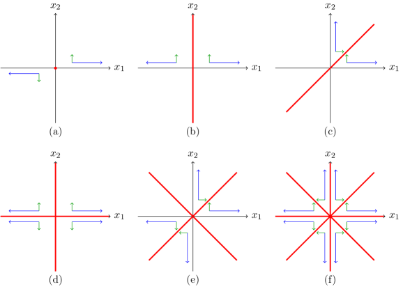
Figure 7: Sketch of the discrete symmetries (a)-(f) respectively given by (LABEL:symmetry-central-second)-(LABEL:symmetry-yamazaki). The axes of symmetry are drawn in red, the first component of $\boldsymbol{f}$ in blue and the second in green.

14 Failure of standard asymptotic expansion

The aim of this paragraph is to show that even in the case the source force $\boldsymbol{f}\in C_{0}^{\infty}(\mathbb{R}^{2})$ has zero mean, inverting the Stokes operator on the nonlinearity in an attempt to solve (LABEL:intro-ns) for $\Omega=\mathbb{R}^{2}$ leads to fundamental problems concerning the behavior at infinity. We consider a source force $\boldsymbol{f}\in C_{0}^{\infty}(\mathbb{R}^{2})$ with zero net force,

$$\int_{\mathbb{R}^{2}}\boldsymbol{f}=\boldsymbol{0}\,.$$

By iteratively inverting the Stokes operator the aim is to generate an expansion in term of $\nu$ of the solution $\boldsymbol{u}$ of (LABEL:intro-ns) with the source term $\boldsymbol{f}$ multiplied by $\nu$,

$$\Delta\boldsymbol{u}-\boldsymbol{\nabla}p =\boldsymbol{u}\boldsymbol{\cdot}\boldsymbol{\nabla}\boldsymbol{u}+\nu\boldsymbol{f}\,, \boldsymbol{\nabla}\boldsymbol{\cdot}\boldsymbol{u} =0\,,$$

in the form

$$\boldsymbol{u}\approx\sum_{n=1}^{\infty}\nu^{n}\boldsymbol{u}_{n}\qquad\text{as}\qquad\nu\approx 0\,.$$

The following result shows that the successive iterates $\boldsymbol{u}_{n}$ decay in general less and less at infinity, so the question of the convergence of the previous series is highly nontrivial.

Proposition 3.5.

The first order has the following asymptotic expansion,

$$\boldsymbol{u}_{1} =\frac{-1}{4\pi r}\left[A\cos(2\theta)\boldsymbol{e}_{r}+B\sin(2\theta)\boldsymbol{e}_{r}+M\boldsymbol{e}_{\theta}\right]+O(r^{-2+\varepsilon})\,,$$

$$p_{1} =\frac{1}{2\pi r^{2}}\left(A\cos(2\theta)+B\sin(2\theta)\right)+O(r^{-3+\varepsilon})\,,$$

for any $\varepsilon>0$, the second order satisfies

$$\boldsymbol{u}_{2} =\frac{M\log r}{2(4\pi)^{2}r}\left(A\sin(2\theta)-B\cos(2\theta)\right)\boldsymbol{e}_{r}+O(r^{-1})\,,$$

$$p_{2} =\frac{M\log r}{(4\pi)^{2}r^{2}}\left(A\sin(2\theta)-B\cos(2\theta)\right)+O(r^{-2})\,,$$

and finally, the expansion of the third order is given by

$$\boldsymbol{u}_{3} =\frac{M^{2}\log^{2}r}{(8\pi)^{3}r}\left(A\cos(2\theta)+B\sin(2\theta)\right)\boldsymbol{e}_{r}+O(r^{-1}\log r)\,,$$

$$p_{3} =\frac{2M^{2}\log^{2}r}{(8\pi)^{3}r^{2}}\left(A\cos(2\theta)+B\sin(2\theta)\right)+O(r^{-1}\log r)\,,$$

for $M\neq 0$ and by

$$\boldsymbol{u}_{3} =-\frac{\left(A^{2}+B^{2}\right)\log r}{12(8\pi)^{3}r}\left(A\cos(2\theta)+B\sin(2\theta)\right)\boldsymbol{e}_{r}+O(r^{-1})\,,$$

$$p_{3} =-\frac{\left(A^{2}+B^{2}\right)\log r}{12(8\pi)^{3}r^{2}}\left(A\cos(2\theta)+B\sin(2\theta)\right)+O(r^{-1})\,,$$

for $M=0$. The constants $A,B,M\in\mathbb{R}$ are given by

$$A =\int_{\mathbb{R}^{2}}\left(x_{1}f_{1}-x_{2}f_{2}\right)\,, B =\int_{\mathbb{R}^{2}}\left(x_{1}f_{2}+x_{2}f_{1}\right)\,, M =\int_{\mathbb{R}^{2}}\left(x_{1}f_{2}-x_{2}f_{1}\right)\,.$$

Therefore, unless $A=B=0$, the third order does not decay like $r^{-1}$ and therefore decays less than the Stokes solution $\boldsymbol{u}_{1}$.

Proof.

The first order is given by the solution of the Stokes equation,

$$\Delta\boldsymbol{u}_{1}-\boldsymbol{\nabla}p_{1} =\boldsymbol{f}\,, \boldsymbol{\nabla}\boldsymbol{\cdot}\boldsymbol{u}_{1} =0\,.$$

By using the asymptotic expansion of the solution of the Stokes equation obtained in lin-stokes-asy,lin-stokes-asy-explicit, we have

$$\boldsymbol{u}_{1} =\boldsymbol{S}_{1}+\boldsymbol{R}_{1}\,,$$

$$p_{1} =s_{1}+r_{1}\,,$$

where $\boldsymbol{S}_{1}\in\mathcal{B}_{1,1}$, $\boldsymbol{R}_{1}\in\mathcal{B}_{1,2}$, $s_{1}\in\mathcal{B}_{0,2}$ and $r_{1}\in\mathcal{B}_{0,3}$. Explicitly, we have

$$\boldsymbol{S}_{1} =\boldsymbol{C}_{1}\boldsymbol{\cdot}\mathbf{E}_{1}\,, s_{1} =\boldsymbol{C}_{1}\boldsymbol{\cdot}\boldsymbol{e}_{1}\,,$$

where $\boldsymbol{C}_{1}=\left(A,B,M\right)\in\mathbb{R}^{3}$ and

$$\mathbf{E}_{1} =\boldsymbol{\nabla}\boldsymbol{\wedge}\left(\chi\boldsymbol{\Psi}_{1}\right)\,, \boldsymbol{\Psi}_{1} =\frac{1}{8\pi}\bigl{(}\sin(2\theta),\>-\cos(2\theta),\>1-2\log r\bigr{)}\,,$$

$$\boldsymbol{e}_{1}=\frac{\chi}{2\pi r^{2}}\bigl{(}\cos(2\theta),\>\sin(2\theta),\>0\bigr{)}\,.$$

The second order has to satisfy the equation

$$\Delta\boldsymbol{u}_{2}-\boldsymbol{\nabla}p_{2}=\boldsymbol{u}_{1}\boldsymbol{\cdot}\boldsymbol{\nabla}\boldsymbol{u}_{1}\,.$$ (27)

However, since $\boldsymbol{S}_{1}\boldsymbol{\cdot}\boldsymbol{\nabla}\boldsymbol{S}_{1}\in\mathcal{B}_{0,3}$, we cannot apply lin-stokes-asy in order to obtain the asymptotic expansion of $\boldsymbol{u}_{2}$. We make an ansatz that explicitly cancels this term for $r>2$. We make the following ansatz for the stream function,

$$\psi_{2}=f_{2}(\theta)+g_{2}(\theta)\log r\,,$$

and consider the equation for the vorticity

$$\Delta^{2}\psi_{2}=\boldsymbol{\nabla}\boldsymbol{\wedge}\left(\boldsymbol{S}_{1}\boldsymbol{\cdot}\boldsymbol{\nabla}\boldsymbol{S}_{1}\right)\,,$$

for $r>2$. We obtain the following ordinary differential equations,

$$g_{2}^{(4)}+4g_{2}^{(2)} =0\,,$$

$$f_{2}^{(4)}+4f_{2}^{(2)}-4g_{2}^{(2)} =\frac{1}{4\pi^{2}}\left(M-A\sin(2\theta)+B\cos(2\theta)\right)\left(A\cos(2\theta)+B\sin(2\theta)\right)\,.$$

The periodic solutions for $g_{2}$ are

$$g_{2}(\theta)=\lambda_{A}\cos(2\theta)+\lambda_{B}\sin(2\theta)\,.$$

Periodic solutions for $f_{2}$ exist if and only if

$$\lambda_{A} =\frac{AM}{(8\pi)^{2}}\,, \lambda_{B}=\frac{BM}{(8\pi)^{2}}\,,$$

and a particular solution is given by

$$f_{2}(\theta)=\frac{1}{6(16\pi)^{2}}\left(\left(B^{2}-A^{2}\right)\sin(4\theta)+2AB\cos(4\theta)\right)\,.$$

Therefore, by defining

$$\boldsymbol{A}_{2} =\boldsymbol{\nabla}\boldsymbol{\wedge}\left(\chi\psi_{2}\right)\,,$$

$$a_{2} =\frac{\chi}{r^{2}}\left[\left(1-2\log r\right)g_{1}^{\prime}(\theta)-2f_{1}^{\prime}(\theta)-\frac{A^{2}+B^{2}+2M^{2}}{(8\pi)^{2}}\right]\,,$$

we obtain

$$\Delta\boldsymbol{A}_{2}-\boldsymbol{\nabla}a_{2}=\boldsymbol{S}_{1}\boldsymbol{\cdot}\boldsymbol{\nabla}\boldsymbol{S}_{1}+\boldsymbol{\delta}_{2}\,,$$

where $\boldsymbol{\delta}_{2}\in C_{0}^{\infty}(\mathbb{R}^{2})$ has compact support. Now by applying lin-stokes-asy-explicit to (LABEL:nonlinear-Stokes-order2), we obtain

$$\boldsymbol{u}_{2} =\boldsymbol{A}_{2}+\boldsymbol{S}_{2}+\boldsymbol{R}_{2}\,, p_{2} =a_{2}+s_{2}+r_{2}\,,$$

where $\boldsymbol{S}_{2}\in\mathcal{B}_{1,1}$, $\boldsymbol{R}_{2}\in\mathcal{B}_{1,2-\varepsilon}$, $s_{2}\in\mathcal{B}_{0,2}$, and $r_{2}\in\mathcal{B}_{0,3-\varepsilon}$ for all $\varepsilon>0$. Again, we have $\boldsymbol{S}_{2}=\boldsymbol{C}_{2}\boldsymbol{\cdot}\mathbf{E}_{1}$ and $s_{2}=\boldsymbol{C}_{2}\boldsymbol{\cdot}\boldsymbol{e}_{1}$ where $\boldsymbol{C}_{2}\in\mathbb{R}^{3}$. The terms $\boldsymbol{A}_{2}$ and $a_{2}$ contain explicit logarithms when $M\neq 0$ and $A^{2}+B^{2}\neq 0$,

$$\boldsymbol{u}_{2} =\frac{M\log r}{2(4\pi)^{2}r}\left(A\sin(2\theta)-B\cos(2\theta)\right)\boldsymbol{e}_{r}+O(r^{-1})\,,$$

$$p_{2} =\frac{M\log r}{(4\pi)^{2}r^{2}}\left(A\sin(2\theta)-B\cos(2\theta)\right)+O(r^{-2})\,.$$

In case where $M=0$, the second order has no logarithm, i.e. $\boldsymbol{u}_{2}\in\mathcal{B}_{1,1}$ and $p_{2}\in\mathcal{B}_{0,2}$. However, we will see that the third order has logarithms as soon as $A^{2}+B^{2}\neq 0$. The third order has to satisfy

$$\Delta\boldsymbol{u}_{3}-\boldsymbol{\nabla}p_{3}=\boldsymbol{u}_{1}\boldsymbol{\cdot}\boldsymbol{\nabla}\boldsymbol{u}_{2}+\boldsymbol{u}_{2}\boldsymbol{\cdot}\boldsymbol{\nabla}\boldsymbol{u}_{1}\,.$$

In the same spirit as before, we make an ansatz in order to explicitly cancel the terms of the right-hand-side that are not $o(r^{-3})$. We make the following ansatz for the approximated stream function at third order,

$$\psi_{3}=f_{3}(\theta)+g_{3}(\theta)\log r+h_{3}(\theta)\log^{2}r\,.$$

The periodic solutions are given by

$$h_{3}(\theta) =\frac{M}{32\pi}g_{2}^{\prime}(\theta)\,,$$

$$g_{3}(\theta) =\frac{M}{16\pi}f_{2}^{\prime}(\theta)+\frac{A^{2}+B^{2}-6M^{2}}{3(16\pi)^{3}}\left(A\sin(2\theta)-B\cos(2\theta)\right)$$

$$\phantom{=}+\frac{M}{2(4\pi)^{2}}\left(C_{21}\cos(2\theta)+C_{22}\sin(2\theta)\right)\,,$$

$$f_{3}(\theta) =\frac{1}{9(32\pi)^{3}}\left(B\left(B^{2}-3A^{2}\right)\cos(6\theta)+A\left(A^{2}-3B^{2}\right)\sin(6\theta)\right)$$

$$\phantom{=}+\frac{1}{6(8\pi)^{2}}\left(\left(AC_{22}+BC_{21}\right)\cos(4\theta)+\left(BC_{22}-AC_{21}\right)\sin(4\theta\right)\,.$$

Therefore, by defining $\boldsymbol{A}_{3}=\boldsymbol{\nabla}\boldsymbol{\wedge}\left(\chi\psi_{3}\right)$ and $a_{3}$ as a suitable pressure that we do not write here explicitly, we obtain that

$$\Delta\boldsymbol{A}_{3}-\boldsymbol{\nabla}a_{3}=\boldsymbol{S}_{1}\boldsymbol{\cdot}\boldsymbol{\nabla}\left(\boldsymbol{A}_{2}+\boldsymbol{S}_{2}\right)+\left(\boldsymbol{A}_{2}+\boldsymbol{S}_{2}\right)\boldsymbol{\cdot}\boldsymbol{\nabla}\boldsymbol{S}_{1}+\boldsymbol{\delta}_{3}\,,$$

where $\boldsymbol{\delta}_{3}\in C_{0}^{\infty}(\mathbb{R}^{2})$. We then obtain the following asymptotic expansion for $\boldsymbol{u}_{3}$,

$$\boldsymbol{u}_{3} =\boldsymbol{A}_{3}+\boldsymbol{C}_{3}\boldsymbol{\cdot}\mathbf{E}_{1}+\boldsymbol{R}_{3}\,, p_{3} =a_{3}+\boldsymbol{C}_{3}\boldsymbol{\cdot}\boldsymbol{e}_{1}+r_{2}\,,$$

where $\boldsymbol{C}_{3}\in\mathbb{R}^{3}$ and $\boldsymbol{R}_{3}\in\mathcal{B}_{1,2-2\varepsilon}$, $r_{3}\in\mathcal{B}_{0,3-2\varepsilon}$ for all $\varepsilon>0$. By explicit calculations, the asymptotic expansion of the third order is proven. ∎

15 Navier-Stokes equations with compatibility conditions

We look at strong solutions to the stationary Navier-Stokes equations in $\mathbb{R}^{2}$,

$$\Delta\boldsymbol{u}-\boldsymbol{\nabla}p -\boldsymbol{u}\boldsymbol{\cdot}\boldsymbol{\nabla}\boldsymbol{u}=\boldsymbol{f}\,, \boldsymbol{\nabla}\boldsymbol{\cdot}\boldsymbol{u} =0\,, \lim_{|\boldsymbol{x}|\to\infty}\boldsymbol{u} =\boldsymbol{0}\,,$$ (28)

and show that for source-terms $\boldsymbol{f}$ with zero mean and in a space of co-dimension three, the Navier-Stokes equations admit a solution decaying like $\left|\boldsymbol{x}\right|^{-2}$:

Theorem 3.6.

For all $\varepsilon\in\left(0,1\right)$, there exists $\nu>0$ such that for any $\boldsymbol{k}\in\mathcal{B}_{0,4+\varepsilon}$ satisfying

$$\left\|\boldsymbol{k};\mathcal{B}_{0,4+\varepsilon}\right\| \leq\nu\,, \int_{\mathbb{R}^{2}}\boldsymbol{k} =\boldsymbol{0}\,,$$

there exists $\boldsymbol{a}\in\mathbb{R}^{3}$ such that there exists $\boldsymbol{u}$ and $p$ satisfying (LABEL:ns-force) with

$$\boldsymbol{f}=\boldsymbol{k}+\frac{\mathrm{e}^{-\left|\boldsymbol{x}\right|{}^{2}}}{\pi}\left[a_{1}\left(x_{1},-x_{2}\right)+a_{2}\left(x_{2},x_{1}\right)+a_{3}\left(-x_{2},x_{1}\right)\right]\,.$$

Moreover, there exists $\boldsymbol{A}\in\mathbb{R}^{4}$ such that

$$\boldsymbol{u} =\frac{A_{1}}{4\pi r^{2}}\bigl{(}\cos(2\theta),\>\sin(2\theta)\bigr{)}+\frac{A_{2}}{4\pi r^{2}}\bigl{(}\sin(2\theta),\>-\cos(2\theta)\bigr{)}$$

$$\phantom{=}+\frac{A_{3}}{4\pi r^{2}}\bigl{(}\cos(2\theta)+\cos(4\theta),\>\sin(4\theta)\bigr{)}+\frac{A_{4}}{4\pi r^{2}}\bigl{(}\sin(2\theta)+\sin(4\theta),\>-\cos(4\theta)\bigr{)}+O(r^{-2-\varepsilon})\,.$$

Proof.

We perform a fixed point argument on $\boldsymbol{u}$ in the space $\mathcal{B}_{1,2}$. We have

$$\Delta\boldsymbol{u}-\boldsymbol{\nabla}p =\boldsymbol{N}\,, \boldsymbol{\nabla}\boldsymbol{\cdot}\boldsymbol{u} =0\,,$$ (29)

with

$$\boldsymbol{N}=\boldsymbol{f}+\boldsymbol{\nabla}\boldsymbol{\cdot}\left(\boldsymbol{u}\otimes\boldsymbol{u}\right)\,.$$

By using lin-stokes-asy-explicit, the compatibility conditions for the solution $\boldsymbol{u}$ of the Stokes system (LABEL:compatibility-stokes-N) to decay faster than $r^{-1}$ are $\boldsymbol{C}_{0}[\boldsymbol{N}]=\boldsymbol{0}$ and $\boldsymbol{C}_{1}[\boldsymbol{N}]=\boldsymbol{0}$. By using the explicit form of $\boldsymbol{N}$, we have

$$\boldsymbol{C}_{0}[\boldsymbol{N}] =\boldsymbol{0}\,, \boldsymbol{C}_{1}[\boldsymbol{N}] =\boldsymbol{a}+\Lambda(\boldsymbol{u})\,,$$

where

$$\Lambda(\boldsymbol{u})=\int_{\mathbb{R}^{2}}\bigl{(}x_{1}k_{1}-x_{2}k_{2}-u_{1}u_{1}+u_{2}u_{2},\,x_{1}k_{2}+x_{2}k_{1}-2u_{1}u_{2},\,x_{1}k_{2}-x_{2}k_{1}\bigr{)}\,.$$

By defining $\boldsymbol{a}=-\Lambda(\boldsymbol{u})$, the compatibility conditions of the Stokes system are satisfied, and since $\boldsymbol{N}\in\mathcal{B}_{0,4+\varepsilon}$, then lin-stokes-asy proves that $\boldsymbol{u}\in\mathcal{B}_{1,2}$.

Since,

$$\left|\Lambda(\boldsymbol{u})\right| \leq 6\left\|\boldsymbol{k};\mathcal{B}_{0,4+\varepsilon}\right\|\int_{\mathbb{R}^{2}}\frac{1}{1+\left|\boldsymbol{x}\right|^{3+\varepsilon}}\mathrm{d}^{2}\boldsymbol{x}+3\left\|\boldsymbol{u};\mathcal{B}_{0,2}\right\|^{2}\int_{\mathbb{R}^{2}}\frac{1}{1+\left|\boldsymbol{x}\right|^{4}}\mathrm{d}^{2}\boldsymbol{x}$$

$$\leq 8\left\|\boldsymbol{k};\mathcal{B}_{0,4+\varepsilon}\right\|+3\left\|\boldsymbol{u};\mathcal{B}_{0,2}\right\|^{2},$$

we have

$$\left\|\boldsymbol{N};\mathcal{B}_{0,4+\varepsilon}\right\| \leq\left\|\boldsymbol{k};\mathcal{B}_{0,4+\varepsilon}\right\|+\left\|\boldsymbol{u};\mathcal{B}_{1,2}\right\|^{2}+\left|\Lambda(\boldsymbol{u})\right|$$

$$\leq 9\left\|\boldsymbol{k};\mathcal{B}_{0,4+\varepsilon}\right\|+4\left\|\boldsymbol{u};\mathcal{B}_{1,2}\right\|^{2}.$$

By hypothesis $\left\|\boldsymbol{k};\mathcal{B}_{0,4+\varepsilon}\right\|\leq\nu$, so by taking $\varepsilon>0$ small enough, we can perform a fixed point argument which shows that the Navier-Stokes system admits a solution $\boldsymbol{u}\in\mathcal{B}_{1,2}$.

Moreover, by using lin-stokes-asy and the explicit form shown in lin-stokes-asy-explicit, the asymptotic behavior is proven. ∎

Under symmetry (LABEL:symmetry-yamazaki) sketched on symmetriesf, the compatibility conditions $\boldsymbol{C}_{0}[\boldsymbol{N}]=\boldsymbol{0}$ and $\boldsymbol{C}_{1}[\boldsymbol{N}]=\boldsymbol{0}$ are satisfied for $a_{1}=a_{2}=a_{3}=0$, so the previous theorem shows that $\boldsymbol{u}$ decays faster than $r^{-2}$:

Corollary 3.7.

For all $\varepsilon\in\left(0,1\right)$, there exists $\nu>0$ such that for any $\boldsymbol{f}\in\mathcal{B}_{0,4+\varepsilon}$ satisfying

$$\left\|\boldsymbol{f};\mathcal{B}_{0,4+\varepsilon}\right\| \leq\nu\,, \int_{\mathbb{R}^{2}}\boldsymbol{f} =\boldsymbol{0}\,,$$

and the symmetry conditions (LABEL:symmetry-galdi) and (LABEL:symmetry-yamazaki), there exists $\boldsymbol{u}$ and $p$ satisfying (LABEL:ns-force), and moreover $\boldsymbol{u}=O(r^{-2-\varepsilon})$ and $p=O(r^{-3-\varepsilon})$.

Proof.

Since $\boldsymbol{f}$ satisfies the symmetry conditions (LABEL:symmetry-galdi) and (LABEL:symmetry-yamazaki), due to the invariance of the Navier-Stokes equation under axial symmetries (LABEL:axial-symmetry), $\boldsymbol{u}$ satisfies the same symmetry conditions, as well as the nonlinearity $\boldsymbol{u}\boldsymbol{\cdot}\boldsymbol{\nabla}\boldsymbol{u}$. Therefore, we can apply strong-under-compatibility with $\boldsymbol{f}=\boldsymbol{k}$ and $\boldsymbol{a}=\boldsymbol{0}$ i.e. $\Lambda(\boldsymbol{u})=\boldsymbol{0}$. ∎

The exact solution $\frac{-M}{4\pi r}\boldsymbol{e}_{\theta}$ of the Navier-Stokes equations generates a net torque and therefore can be used to lift the third component of $\boldsymbol{C}_{1}[\boldsymbol{N}]$ corresponding to the net torque. More precisely, we can enlarge the class of source terms $\boldsymbol{f}$ to a subspace of co-dimension two:

Theorem 3.8.

For all $\varepsilon\in\left(0,1\right)$, there exists $\nu>0$, such that for any $\boldsymbol{k}\in\mathcal{B}_{0,3+\varepsilon}$ satisfying

$$\left\|\boldsymbol{k};\mathcal{B}_{0,3+\varepsilon}\right\| \leq\nu\,, \int_{\mathbb{R}^{2}}\boldsymbol{k} =\boldsymbol{0}\,,$$

there exists $\boldsymbol{a}\in\mathbb{R}^{2}$ such that there exists $\boldsymbol{u}$ and $p$ satisfying (LABEL:ns-force) with

$$\boldsymbol{f}=\boldsymbol{k}+\frac{\mathrm{e}^{-\left|\boldsymbol{x}\right|{}^{2}}}{\pi}\left[a_{1}\left(x_{1},-x_{2}\right)+a_{2}\left(x_{2},x_{1}\right)\right].$$

Moreover,

$$\boldsymbol{u}=-\frac{M}{4\pi r}\boldsymbol{e}_{\theta}+O(r^{-1-\varepsilon})\,,$$

where

$$M=\int_{\mathbb{R}^{2}}\boldsymbol{x}\boldsymbol{\wedge}\boldsymbol{k}=\int_{\mathbb{R}^{2}}\boldsymbol{x}\boldsymbol{\wedge}\boldsymbol{f}\,.$$

Proof.

In order to lift the compatibility condition corresponding to the net torque, we consider the solution

$$\boldsymbol{u}_{0} =-\frac{M}{4\pi}\boldsymbol{\nabla}\boldsymbol{\wedge}\left(\chi(r)\log(r)\right)\,, p_{0} =\frac{-1}{2}\left(\frac{M\chi(r)}{4\pi r}\right)^{2},$$

which is an exact solution of the Stokes and Navier-Stokes equations for $r\geq 2$. So we have

$$\Delta\boldsymbol{u}_{0}-\boldsymbol{\nabla}p_{0}-\boldsymbol{u}_{0}\boldsymbol{\cdot}\boldsymbol{\nabla}\boldsymbol{u}_{0}=\boldsymbol{f}_{\!0}\,,$$

where $\boldsymbol{f}_{\!0}$ is a source force of compact support. Since $\boldsymbol{u}_{0}$ and $p_{0}$ are invariant under rotations, $\boldsymbol{C}_{0}[\boldsymbol{f}_{\!0}]=\boldsymbol{0}$ and $\boldsymbol{C}_{1}[\boldsymbol{f}_{\!0}]=\left(0,0,*\right)$. To determine the last unknown, we integrate

$$\int_{\mathbb{R}^{2}}\boldsymbol{x}\boldsymbol{\wedge}\boldsymbol{f}_{\!0}=-\frac{M}{2}\int_{0}^{\infty}\left[r\log r\,\chi^{(3)}(r)+\left(\log r+3\right)\chi^{\prime\prime}(r)-\frac{\log r+1}{r}\chi^{\prime}(r)\right]\mathrm{d}r=M\,.$$

Therefore, we have

$$\boldsymbol{C}_{0}[\boldsymbol{f}_{\!0}] =\boldsymbol{0}\,, \boldsymbol{C}_{1}[\boldsymbol{f}_{\!0}] =\left(0,0,-M\right)\,.$$

By writing $\boldsymbol{u}$ and $p$ as $\boldsymbol{u}=\boldsymbol{u}_{0}+\boldsymbol{u}_{1}$, $p=p_{0}+p_{1}$, the Navier-Stokes equations become

$$\Delta\boldsymbol{u}_{1}-\boldsymbol{\nabla}p_{1} =\boldsymbol{N}\,, \boldsymbol{\nabla}\boldsymbol{\cdot}\boldsymbol{u}_{1} =0\,,$$

with

$$\boldsymbol{N}=\boldsymbol{f}+\boldsymbol{\nabla}\boldsymbol{\cdot}\left(\boldsymbol{u}_{0}\otimes\boldsymbol{u}_{1}+\boldsymbol{u}_{1}\otimes\boldsymbol{u}_{0}+\boldsymbol{u}_{1}\otimes\boldsymbol{u}_{1}\right)-\boldsymbol{f}_{\!0}\,.$$

The aim is to perform a fixed point on $\boldsymbol{u}_{1}$ in the space $\mathcal{B}_{1,1+\varepsilon}$. Since $\boldsymbol{f}$ has zero mean by hypothesis, $\boldsymbol{C}_{0}[\boldsymbol{N}]=\boldsymbol{0}$. By defining $M=\int_{\mathbb{R}^{2}}\boldsymbol{x}\boldsymbol{\wedge}\boldsymbol{f}$ and by using invariants, the third component of $\boldsymbol{C}_{1}[\boldsymbol{N}]$, which is the net torque, is given by

$$\int_{\mathbb{R}^{2}}\boldsymbol{x}\boldsymbol{\wedge}\boldsymbol{N} =\int_{\mathbb{R}^{2}}\boldsymbol{\nabla}\boldsymbol{\cdot}\left[\left(\boldsymbol{u}_{0}\otimes\boldsymbol{u}_{1}+\boldsymbol{u}_{1}\otimes\boldsymbol{u}_{0}+\boldsymbol{u}_{1}\otimes\boldsymbol{u}_{1}\right)\boldsymbol{\cdot}\boldsymbol{x}^{\perp}\right]$$

$$=\lim_{R\to\infty}\int_{\partial B(\boldsymbol{0},R)}\boldsymbol{x}^{\perp}\boldsymbol{\cdot}\left(\boldsymbol{u}_{0}\otimes\boldsymbol{u}_{1}+\boldsymbol{u}_{1}\otimes\boldsymbol{u}_{0}+\boldsymbol{u}_{1}\otimes\boldsymbol{u}_{1}\right)\boldsymbol{\cdot}\boldsymbol{n}\,.$$

Since $\boldsymbol{u}_{0}\in\mathcal{B}_{0,1}$ and $\boldsymbol{u}_{1}\in\mathcal{B}_{0,1+\varepsilon}$ , we obtain

$$\left|\int_{\mathbb{R}^{2}}\boldsymbol{x}\boldsymbol{\wedge}\boldsymbol{N}\right|\leq\left\|\boldsymbol{u}_{1};\mathcal{B}_{0,1+\varepsilon}\right\|\left(\left\|\boldsymbol{u}_{0};\mathcal{B}_{0,1}\right\|+\left\|\boldsymbol{u}_{1};\mathcal{B}_{0,1+\varepsilon}\right\|\right)\lim_{R\to\infty}R^{-\varepsilon}=0\,,$$

so the compatibility condition for the net torque is automatically fulfilled. In the same way as in the proof of strong-under-compatibility, we have

$$\boldsymbol{C}_{0}[\boldsymbol{N}] =\boldsymbol{0}\,, \boldsymbol{C}_{1}[\boldsymbol{N}] =\bigl{(}\boldsymbol{a}+\Lambda(\boldsymbol{u}_{1}),0\bigr{)}\,,$$

where

$$\Lambda(\boldsymbol{u}_{1})=\int_{\mathbb{R}^{2}}\bigl{(}x_{1}k_{1}-x_{2}k_{2}-u_{1}u_{1}+u_{2}u_{2},\,x_{1}k_{2}+x_{2}k_{1}-2u_{1}u_{2}\bigr{)}\,.$$

By defining $\boldsymbol{a}=-\Lambda(\boldsymbol{u})$, the compatibility conditions of the Stokes system to decay faster than $r^{-1}$ are satisfied. Therefore, it remains to bound $\boldsymbol{N}$ is order to apply a fixed point argument. We have

$$\left\|\boldsymbol{u}_{0};\mathcal{B}_{1,1}\right\|\lesssim\left|M\right|\lesssim\left\|\boldsymbol{k};\mathcal{B}_{0,3+\varepsilon}\right\|\leq\nu\,,$$

and

$$\left|\Lambda(\boldsymbol{u})\right| \lesssim\left\|\boldsymbol{k};\mathcal{B}_{0,3+\varepsilon}\right\|+\left\|\boldsymbol{u}_{1};\mathcal{B}_{0,1+\varepsilon}\right\|\left(\left\|\boldsymbol{u}_{0};\mathcal{B}_{0,1}\right\|+\left\|\boldsymbol{u}_{1};\mathcal{B}_{0,1+\varepsilon}\right\|\right)$$

$$\lesssim\nu+\nu\left\|\boldsymbol{u}_{1};\mathcal{B}_{0,1+\varepsilon}\right\|+\left\|\boldsymbol{u}_{1};\mathcal{B}_{0,1+\varepsilon}\right\|^{2},$$

so

$$\left\|\boldsymbol{N};\mathcal{B}_{0,4+\nu}\right\| \leq\left\|\boldsymbol{k};\mathcal{B}_{0,3+\varepsilon}\right\|+\left\|\boldsymbol{u}_{1};\mathcal{B}_{1,1+\varepsilon}\right\|\left(\left\|\boldsymbol{u}_{0};\mathcal{B}_{1,1}\right\|+\left\|\boldsymbol{u}_{1};\mathcal{B}_{1,1+\varepsilon}\right\|\right)+\left|\Lambda(\boldsymbol{u})\right|$$

$$\lesssim\nu+\nu\left\|\boldsymbol{u}_{1};\mathcal{B}_{1,1+\varepsilon}\right\|+\left\|\boldsymbol{u}_{1};\mathcal{B}_{1,1+\varepsilon}\right\|^{2}.$$

Consequently, by applying lin-stokes-asy, we can perform a fixed point argument on $\boldsymbol{u}_{1}\in\mathcal{B}_{1,1+\varepsilon}$ which proves the existence of a solution $\boldsymbol{u}=\boldsymbol{u}_{0}+\boldsymbol{u}_{1}$ of the Navier-Stokes system together with the claimed asymptotic behavior, since $\boldsymbol{u}_{0}=\frac{-M}{4\pi r}\boldsymbol{e}_{\theta}$ for $r\geq 2$.∎

Remark 3.9.

This theorem shows that the knowledge of one suitable explicit solution of the Navier-Stokes equations can be used to lift one compatibility condition and enlarge the space of source forces $\boldsymbol{f}$ for which we can solve the problem. The compatibility condition we lifted is the one related to net torque, which is an invariant quantity, so we do not need to adjust $M$ inside the fixed point, i.e. $M$ depends only on $\boldsymbol{f}$ not on $\boldsymbol{u}_{1}$. In the case where we try to lift a compatibility condition that is not a conserved quantity, we would have to adjust the parameter of the explicit solution at each iteration of the fixed point argument.

Remark 3.10.

The method used in this theorem cannot be applied to the case where $\boldsymbol{f}$ has nonzero mean for the following reason. In order to treat the nonlinearity by inverting the Stokes operator on it, the explicit solution $\boldsymbol{u}_{0}$ that lifts the compatibility condition has to be in the space $\mathcal{B}_{1,1}$ and the perturbation $\boldsymbol{u}_{1}$ in $\mathcal{B}_{1,1+\varepsilon}$ for some $\varepsilon>0$, otherwise the inversion of the Stokes operator on the nonlinearity leads to logarithms, and the fixed point argument cannot be closed. But we cannot lift the mean value of the force $\boldsymbol{F}$ with an explicit solution $\boldsymbol{u}_{0}\in\mathcal{B}_{1,1}$: if $\boldsymbol{u}_{0}\in\mathcal{B}_{1,1}$ and $p_{0}\in\mathcal{B}_{0,2}$, we have

$$\mathbf{T}_{0}=\boldsymbol{\nabla}\boldsymbol{u}_{0}+\left(\boldsymbol{\nabla}\boldsymbol{u}_{0}\right)^{T}-p_{0}\mathbf{1}-\boldsymbol{u}_{0}\otimes\boldsymbol{u}_{0}\in\mathcal{B}_{0,2}\,,$$

so by using invariants,

$$\left|\boldsymbol{F}_{0}\right|=\left|\int_{\mathbb{R}^{2}}\boldsymbol{f}_{0}\right|=\lim_{R\to\infty}\biggl{|}\int_{B(\boldsymbol{0},R)}\!\mathbf{T}_{0}\boldsymbol{n}\biggr{|}\leq\left\|\mathbf{T}_{0};\mathcal{B}_{0,2}\right\|\lim_{R\to\infty}R^{-1}=0\,.$$

Chapter 4 On the asymptotes of the Stokes and Navier-Stokes equations

We consider the Navier-Stokes equations in the exterior domain $\Omega=\mathbb{R}^{2}\setminus B$ where $B$ is a compact and simply connected set with smooth boundary,

$$\Delta\boldsymbol{u}-\boldsymbol{\nabla}p =\nu\boldsymbol{u}\boldsymbol{\cdot}\boldsymbol{\nabla}\boldsymbol{u}+\boldsymbol{f}\,, \boldsymbol{\nabla}\boldsymbol{\cdot}\boldsymbol{u} =0\,,$$ (30)

$$\left.\boldsymbol{u}\right|_{\partial B} =\boldsymbol{u}^{*}\,, \lim_{|\boldsymbol{x}|\to\infty}\boldsymbol{u} =\boldsymbol{0}\,,$$

where $\nu\in\mathbb{R}$ is a parameter, $\boldsymbol{u}^{*}$ is a boundary condition and $\boldsymbol{f}$ a source force. These equations admit four invariant quantities (see invariants): the flux $\Phi$, the net force $\boldsymbol{F}$, and the net torque $M$,

$$\Phi= \int_{\partial B}\boldsymbol{u}\boldsymbol{\cdot}\boldsymbol{n}\,, \boldsymbol{F} =\int_{\Omega}\boldsymbol{f}+\int_{\partial B}\mathbf{T}\boldsymbol{n}\,, M =\int_{\Omega}\boldsymbol{x}\boldsymbol{\wedge}\boldsymbol{f}+\int_{\partial B}\boldsymbol{x}\boldsymbol{\wedge}\mathbf{T}\boldsymbol{n}\,,$$

where $\mathbf{T}$ is the stress tensor including the convective part,

$$\mathbf{T}=\boldsymbol{\nabla}\boldsymbol{u}+\left(\boldsymbol{\nabla}\boldsymbol{u}\right)^{T}-p\,\boldsymbol{1}-\nu\boldsymbol{u}\otimes\boldsymbol{u}\,.$$

For $\nu=0$, the system (LABEL:link-ns) is linear and is called the Stokes equations, whereas if $\nu\neq 0$, the equations are the Navier-Stokes equations. Deuring & Galdi (2000) proved that in three dimensions, the solution of the Navier-Stokes equations cannot be asymptotic to the Stokes fundamental solution. The aim of this chapter is to prove an analog result in two dimensions. In contrast to the three-dimensional case, the requirement that the velocity vanishes at infinity imposes that the net force vanishes for the Stokes equations. The asymptotic expansion of the Stokes equations up to order $r^{-1}$ has four real parameters. Moreover, the velocity of the Navier-Stokes equations can be asymptotic only to two of the four terms in $r^{-1}$ of the Stokes asymptote. The existence of such a solution was proven in compatibility-strong-mu. These two terms are the two harmonic functions decaying like $r^{-1}$ and therefore the asymptotic expansion of the pressure up to order $r^{-2}$ cannot coincide since the pressure term of an harmonic function is given by $\frac{\nu}{2}\left|\boldsymbol{u}\right|^{2}$.

The following theorem provides the main result of this chapter:

Theorem 4.1.

Let $\varepsilon\in\left(0,1\right)$, $\nu\in\mathbb{R}$, $\boldsymbol{f}\in C^{0}(\Omega)$ such that $\left(1+\left|\boldsymbol{x}\right|^{3+\varepsilon}\right)\boldsymbol{f}\in L^{\infty}(\Omega)$ and let $\left(\boldsymbol{u},p\right)\in C^{2}(\Omega)\times C^{1}(\Omega)$ be a solution of the Navier-Stokes equations (LABEL:link-ns).

1. If $\nu=0$, then there exists $\boldsymbol{A}=(A_{0},A_{1},A_{2},A_{3})\in\mathbb{R}^{4}$ such that

   $$\boldsymbol{u} =\boldsymbol{u}_{1}+O(r^{-1-\varepsilon})\,, \boldsymbol{\nabla}\boldsymbol{u} =\boldsymbol{\nabla}\boldsymbol{u}_{1}+O(r^{-1-\varepsilon})\,, p =p_{1}+O(r^{-2-\varepsilon})\,,$$

   where

   $$\boldsymbol{u}_{1} =\frac{1}{4\pi r}\left[2A_{0}\boldsymbol{e}_{r}-A_{1}\cos(2\theta)\boldsymbol{e}_{r}-A_{2}\sin(2\theta)\boldsymbol{e}_{r}-A_{3}\boldsymbol{e}_{\theta}\right],$$

   $$p_{1} =\frac{-1}{4\pi r^{2}}\left[A_{1}\cos(2\theta)+A_{2}\sin(2\theta)\right].$$

   Moreover, the net force vanishes, $\boldsymbol{F}=\boldsymbol{0}$, the parameters of the vector $\boldsymbol{A}$ can be expressed in terms of integrals involving $\boldsymbol{u}$ and $\boldsymbol{f}$, and in particular

   $$A_{0} =\Phi\,, A_{3}= M\,.$$

2. If $\nu\neq 0$ and $\boldsymbol{u}$ satisfies

   $$\boldsymbol{u}=\boldsymbol{u}_{1}+O(r^{-1-\varepsilon})\,,$$

   for some $\boldsymbol{A}=(A_{0},A_{1},A_{2},A_{3})\in\mathbb{R}^{4}$, then $A_{1}=A_{2}=0$ and $A_{0}=\Phi$. If in addition $p$ satisfies

   $$p=p_{1}+O(r^{-2-\varepsilon})\,,$$

   then $\Phi=M=0$, so $\boldsymbol{A}=\boldsymbol{0}$ and $\boldsymbol{u}=O(r^{-1-\varepsilon})$. Moreover if

   $$\boldsymbol{\nabla}\boldsymbol{u}=\boldsymbol{\nabla}\boldsymbol{u}_{1}+O(r^{-1-\varepsilon})\,,$$

   then the net force vanishes $\boldsymbol{F}=\boldsymbol{0}$ and the net torque is $M=A_{3}$.

16 Truncation procedure

The aim of this section is to show that by using a cut-off procedure we can get rid of the body and consider modified equations in $\mathbb{R}^{2}$.

Since $B$ is compact, there exits $R>1$ such that $B\subset B(\boldsymbol{0},R)$, where $B(\boldsymbol{0},R)$ is the ball of radius $R$ centered at the origin. We denote by $\chi$ a smooth cut-off function such that $\chi(r)=0$ for $0\leq r\leq R$ and $\chi(r)=1$ if $r\geq 2R$. The flux is defined by

$$\Phi=\int_{\partial B}\boldsymbol{u}\boldsymbol{\cdot}\boldsymbol{n}\,.$$

To deal with the flux in $\mathbb{R}^{2}$, we define the following smooth flux carrier,

$$\boldsymbol{\Sigma} =\frac{\chi(r)}{2\pi r}\boldsymbol{e}_{r}\,, \sigma =\frac{\chi^{\prime}(r)}{2\pi r}\,,$$

which is smooth in $\mathbb{R}^{2}$ and an exact solution of (LABEL:link-ns) for $\nu=0$ in $\mathbb{R}^{2}\setminus B(\boldsymbol{0},2R)$ with $\boldsymbol{f}=\boldsymbol{0}$ and $\boldsymbol{u}^{*}=\frac{\boldsymbol{e}_{r}}{2\pi r}$.

Proposition 4.2.

Let $\left(\boldsymbol{u},p\right)\in C^{2}(\Omega)\times C^{1}(\Omega)$ be a solution of (LABEL:link-ns). Then there exists a solution $\left(\bar{\boldsymbol{u}},\bar{p}\right)\in C^{2}(\mathbb{R}^{2})\times C^{1}(\mathbb{R}^{2})$ of

$$\Delta\bar{\boldsymbol{u}}-\boldsymbol{\nabla}\bar{p} =\nu\bar{\boldsymbol{u}}\boldsymbol{\cdot}\boldsymbol{\nabla}\bar{\boldsymbol{u}}+\bar{\boldsymbol{f}}\,, \boldsymbol{\nabla}\boldsymbol{\cdot}\bar{\boldsymbol{u}} =\Phi\boldsymbol{\nabla}\boldsymbol{\cdot}\boldsymbol{\Sigma}\,, \lim_{\left|\boldsymbol{x}\right|\to\infty} \boldsymbol{u}=\boldsymbol{0}\,,$$ (31)

in $\mathbb{R}^{2}$ such that $\boldsymbol{u}=\bar{\boldsymbol{u}}$, $p=\bar{p}$, and $\boldsymbol{f}=\bar{\boldsymbol{f}}$ in $\mathbb{R}^{2}\setminus B(\boldsymbol{0},2R)$.

Proof.

First of all let $\boldsymbol{v}=\boldsymbol{u}-\Phi\boldsymbol{\Sigma}$ and $q=p-\Phi\sigma$ so that $\boldsymbol{v}$ has zero flux,

$$\int_{\partial B(\boldsymbol{0},R)}\boldsymbol{v}\boldsymbol{\cdot}\boldsymbol{n}=\int_{\partial B}\boldsymbol{u}\boldsymbol{\cdot}\boldsymbol{n}-\Phi\int_{\partial B(\boldsymbol{0},R)}\boldsymbol{\Sigma}\boldsymbol{\cdot}\boldsymbol{n}=0\,,$$

and therefore the function

$$\psi(\boldsymbol{x})=\int_{\gamma(\boldsymbol{x})}\boldsymbol{v}^{\perp}\boldsymbol{\cdot}\mathrm{d}\boldsymbol{x}\,,$$

where $\gamma(\boldsymbol{x})$ is any smooth curve connecting $\left(R,0\right)$ to $\boldsymbol{x}$ is a stream function for $\boldsymbol{v}$, i.e. $\boldsymbol{v}=\boldsymbol{\nabla}\boldsymbol{\wedge}\psi$ in $\mathbb{R}^{2}\setminus B(\boldsymbol{0},R)$. Since $\psi\in C^{2}(\mathbb{R}^{2}\setminus B(\boldsymbol{0},R))$, by defining

$$\bar{\boldsymbol{u}} =\Phi\boldsymbol{\Sigma}+\bar{\boldsymbol{v}}\,, \bar{\boldsymbol{v}} =\boldsymbol{\nabla}\boldsymbol{\wedge}\left(\chi\psi\right)\,, \bar{p} =\Phi\sigma+\chi q\,,$$

we have $\left(\bar{\boldsymbol{u}},\bar{p}\right)\in C^{2}(\mathbb{R}^{2})\times C^{1}(\mathbb{R}^{2})$, $\bar{\boldsymbol{u}}=\boldsymbol{u}$ and $\bar{p}=p$ for $r\geq 2R$. By plugging $\left(\bar{\boldsymbol{u}},\bar{p}\right)$ into (LABEL:ns-plane), we obtain

$$\Delta\bar{\boldsymbol{u}}-\boldsymbol{\nabla}\bar{p}-\nu\bar{\boldsymbol{u}}\boldsymbol{\cdot}\boldsymbol{\nabla}\bar{\boldsymbol{u}} =\chi\boldsymbol{f}+\boldsymbol{\delta}\,, \boldsymbol{\nabla}\boldsymbol{\cdot}\bar{\boldsymbol{u}} =\Phi\boldsymbol{\nabla}\boldsymbol{\cdot}\boldsymbol{\Sigma}\,,$$

where $\boldsymbol{\delta}\in C_{0}^{1}(\mathbb{R}^{2})$ and $\boldsymbol{\nabla}\boldsymbol{\cdot}\boldsymbol{\Sigma}\in C_{0}^{\infty}(\mathbb{R}^{2})$ have support only on $B(\boldsymbol{0},2R)$. The proposition is proved by taking $\bar{\boldsymbol{f}}=\chi\boldsymbol{f}+\boldsymbol{\delta}$. ∎

17 Stokes equations

In this section, we prove the first part of the theorem concerning the linear case: $\nu=0$. We first define weighted $L^{\infty}$-spaces:

Definition 4.3 (function spaces).

For $q\geq 0$, we define the weight

$$w_{q}(\boldsymbol{x})=\begin{cases}1+\left|\boldsymbol{x}\right|^{q}\,,&q>0\,,\\ \left[\log\left(2+\left|\boldsymbol{x}\right|\right)\right]^{-1}\,,&q=0\,,\end{cases}$$

and the associated Banach space for $k\in\mathbb{N}$,

$$\mathcal{B}_{k,q}=\left\{f\in C^{k}(\mathbb{R}^{n})\,:\>w_{q+\left|\alpha\right|}D^{\alpha}f\in L^{\infty}(\mathbb{R}^{n})\>\forall\left|\alpha\right|\leq k\right\},$$

with the norm

$$\bigl{\|}f;\mathcal{B}_{k,q}\bigr{\|}=\max_{\left|\alpha\right|\leq k}\sup_{\boldsymbol{x}\in\mathbb{R}^{n}}w_{q+\left|\sigma\right|}\left|D^{\alpha}f\right|\,.$$

Proposition 4.4.

If $\bar{\boldsymbol{f}}\in\mathcal{B}_{0,3+\varepsilon}$ for $\varepsilon\in\left(0,1\right)$, the solution of (LABEL:ns-plane) with $\nu=0$ satisfies

$$\bar{\boldsymbol{u}} =\bar{\boldsymbol{u}}_{1}+\tilde{\boldsymbol{u}}\,, \bar{p} =\bar{p}_{1}+\tilde{p}\,,$$

where $\tilde{\boldsymbol{u}}\in\mathcal{B}_{1,1+\varepsilon}$, $\tilde{p}\in\mathcal{B}_{0,2+\varepsilon}$, and

$$\bar{\boldsymbol{u}}_{1} =\boldsymbol{A}\boldsymbol{\cdot}\left(\boldsymbol{\Sigma},\mathbf{E}_{1}\right)\,, \bar{p}_{1} =\boldsymbol{A}\boldsymbol{\cdot}\left(\sigma,\boldsymbol{e}_{1}\right)\,,$$

for some $\boldsymbol{A}\in\mathbb{R}^{4}$, with $A_{0}=\Phi$. The first order of the asymptotic expansion $\mathbf{E}_{1}$ (which is a tensor of type $\left(2,3\right)$) and $\boldsymbol{e}_{1}$ are defined in lin-stokes-asy-explicit.

Proof.

By plugging $\bar{\boldsymbol{u}}=\Phi\boldsymbol{\Sigma}+\bar{\boldsymbol{v}}$ and $\bar{p}=\Phi\sigma+\bar{q}$ in (LABEL:ns-plane), we obtain

$$\Delta\bar{\boldsymbol{v}}-\boldsymbol{\nabla}\bar{q} =\bar{\boldsymbol{f}}\,, \boldsymbol{\nabla}\boldsymbol{\cdot}\bar{\boldsymbol{v}} =\boldsymbol{0}\,.$$

By lin-stokes-asy, we have

$$\bar{\boldsymbol{v}} =\boldsymbol{S}_{0}+\boldsymbol{S}_{1}+\tilde{\boldsymbol{u}}\,, \bar{q} =s_{0}+s_{1}+\tilde{p}\,,$$

where $\boldsymbol{S}_{i}\in\mathcal{B}_{1,i}$, $\tilde{\boldsymbol{u}}\in\mathcal{B}_{1,1+\varepsilon}$, $s_{i}\in\mathcal{B}_{0,i+1}$ and $\tilde{p}\in\mathcal{B}_{0,2+\varepsilon}$. In particular, by using lin-stokes-asy-explicit, the terms are given by

$$\boldsymbol{S}_{0} =\boldsymbol{C}_{0}\boldsymbol{\cdot}\mathbf{E}_{0}\,, s_{0} =\boldsymbol{C}_{0}\boldsymbol{\cdot}\boldsymbol{e}_{0}\,,$$

$$\boldsymbol{S}_{1} =\boldsymbol{C}_{1}\boldsymbol{\cdot}\mathbf{E}_{1}\,, s_{1} =\boldsymbol{C}_{1}\boldsymbol{\cdot}\boldsymbol{e}_{1}\,,$$

where $\boldsymbol{C}_{0},\boldsymbol{C}_{1}\in\mathbb{R}^{3}$ are given by integrals of $\bar{\boldsymbol{f}}$. The term $\mathbf{E}_{0}$ grows at infinity like $\log r$ and since the velocity has to be zero at infinity, the term $\boldsymbol{S}_{0}$ has to vanish, so $\boldsymbol{C}_{0}=\boldsymbol{0}$. ∎

18 Navier-Stokes equations

In this section we prove the second part of the theorem concerning the case where $\nu\neq 0$. The term $\bar{\boldsymbol{u}}_{1}\in\mathcal{B}_{1,1}$ generates a nonlinear term $\nu\bar{\boldsymbol{u}}_{1}\boldsymbol{\cdot}\boldsymbol{\nabla}\bar{\boldsymbol{u}}_{1}\in\mathcal{B}_{0,3}$, so we cannot apply stokes to solve the following Stokes system,

$$\Delta\bar{\boldsymbol{u}}_{2}-\boldsymbol{\nabla}\bar{p}_{2} =\nu\bar{\boldsymbol{u}}_{1}\boldsymbol{\cdot}\boldsymbol{\nabla}\bar{\boldsymbol{u}}_{1}\,, \boldsymbol{\nabla}\boldsymbol{\cdot}\bar{\boldsymbol{u}}_{2} =0\,.$$

In the following key lemma, we explicitly construct a solution to this system up to a compactly supported function and determine its asymptotic behavior.

Lemma 4.5.

There exists a smooth solution $\left(\bar{\boldsymbol{u}}_{2},\bar{p}_{2}\right)$ of the equations

$$\Delta\bar{\boldsymbol{u}}_{2}-\boldsymbol{\nabla}\bar{p}_{2} =\nu\bar{\boldsymbol{u}}_{1}\boldsymbol{\cdot}\boldsymbol{\nabla}\bar{\boldsymbol{u}}_{1}+\boldsymbol{\delta}_{2}\,, \boldsymbol{\nabla}\boldsymbol{\cdot}\bar{\boldsymbol{u}}_{2} =0\,,$$

in $\mathbb{R}^{2}$ where $\boldsymbol{\delta}_{2}\in C_{0}^{1}(\mathbb{R}^{2})$ has compact support, such that for $r\geq 2R$,

$$\bar{\boldsymbol{u}}_{2} =\frac{\nu\mathcal{A}_{1}\mathcal{A}_{2}}{(8\pi)^{2}r}\left[\log r\,\sin\left(2\theta+\theta_{1}\right)\boldsymbol{e}_{r}+\cos\left(2\theta+\theta_{1}\right)\boldsymbol{e}_{\theta}\right]+\frac{\nu\mathcal{A}_{1}^{2}}{6(8\pi)^{2}r}\sin(4\theta+\theta_{2})\boldsymbol{e}_{r}$$ (32)

$$\bar{p}_{2} =\frac{\nu\mathcal{A}_{1}\mathcal{A}_{2}}{32\pi^{2}r^{2}}\left(2\log r-1\right)\sin\left(2\theta+\theta_{1}\right)+\frac{\nu\mathcal{A}_{1}^{2}}{3(8\pi)^{2}r^{2}}\sin(4\theta+\theta_{2})-\frac{\nu\left(\mathcal{A}_{1}^{2}+\mathcal{A}_{2}^{2}\right)}{(8\pi)^{2}r^{2}}\,,$$

where

$$\mathcal{A}_{1} =\sqrt{A_{1}^{2}+A_{2}^{2}}\,, \mathcal{A}_{2} =\sqrt{4A_{0}^{2}+A_{3}}\,,$$

and $\theta_{1}$, $\theta_{2}$ are angles related to $A_{1}$ and $A_{2}$.

Proof.

We make an ansatz that explicitly cancel this term for $r>2R$. We make the following ansatz for the stream function,

$$\psi_{2}=f_{2}(\theta)+g_{2}(\theta)\log r\,,$$

and consider the equation of the vorticity

$$\Delta^{2}\psi_{2}=\boldsymbol{\nabla}\boldsymbol{\wedge}\left(\nu\bar{\boldsymbol{u}}_{1}\boldsymbol{\cdot}\boldsymbol{\nabla}\bar{\boldsymbol{u}}_{1}\right)\,,$$

for $r>2R$. We obtain the following ordinary differential equations,

$$g_{2}^{(4)}+4g_{2}^{(2)} =0\,,$$

$$f_{2}^{(4)}+4f_{2}^{(2)}-4g_{2}^{(2)} =\frac{\nu\mathcal{A}_{1}}{8\pi^{2}}\left[2\mathcal{A}_{2}\cos(2\theta+\theta_{1})+\mathcal{A}_{1}\cos(4\theta+\theta_{2})\right],$$

where $\theta_{2}$ and $\theta_{4}$ are angles expressed in terms of $A$ and $B$. The periodic solutions for $g_{2}$ are

$$g_{2}(\theta)=\lambda\cos(2\theta+\theta_{0})\,.$$

Periodic solutions for $f_{2}$ exist if and only if

$$\lambda =\frac{\nu\mathcal{A}_{1}\mathcal{A}_{2}}{(8\pi)^{2}}\,, \theta_{0}=\theta_{2}\,,$$

and a particular solution is given by

$$f_{2}(\theta)=\frac{\nu\mathcal{A}_{1}^{2}}{6(16\pi)^{2}}\left(\cos(4\theta+\theta_{2})\right).$$

Therefore, by defining

$$\bar{\boldsymbol{u}}_{2} =\boldsymbol{\nabla}\boldsymbol{\wedge}\left(\chi\psi_{2}\right),$$

$$\bar{p}_{2} =\frac{\nu\chi}{r^{2}}\left[\left(1-2\log r\right)g_{1}^{\prime}(\theta)-2f_{1}^{\prime}(\theta)-\frac{\mathcal{A}_{1}^{2}+2\mathcal{A}_{2}^{2}}{(8\pi)^{2}}\right],$$

the lemma is proven. ∎

By applying this lemma we obtain:

Proposition 4.6.

Let $\varepsilon\in(0,1)$, $\bar{\boldsymbol{f}}\in\mathcal{B}_{0,3+\varepsilon}$ and $\left(\bar{\boldsymbol{u}},\bar{p}\right)\in C^{2}(\Omega)\times C^{1}(\Omega)$ be a solution of (LABEL:ns-plane) for $\nu\neq 0$. If $\bar{\boldsymbol{u}}$ is asymptotic to the solution of the Stokes equations, i.e.

$$\bar{\boldsymbol{u}}=\boldsymbol{A}\boldsymbol{\cdot}\left(\boldsymbol{\Sigma},\mathbf{E}_{1}\right)+\tilde{\boldsymbol{u}}\,,$$

for some $\boldsymbol{A}=\left(A_{0},A_{1},A_{2},A_{3}\right)\in\mathbb{R}^{4}$ and $\tilde{\boldsymbol{u}}\in\mathcal{B}_{0,1+\varepsilon}$ then $A_{0}=\Phi$ and $A_{1}=A_{2}=0$. Moreover if $\bar{p}$ is asymptotic to the solution of the stokes equations, i.e.

$$\bar{p}=\boldsymbol{A}\boldsymbol{\cdot}\left(\boldsymbol{\Sigma},\mathbf{E}_{1}\right)+\tilde{p}$$

for some $\tilde{p}\in\mathcal{B}_{0,2+\varepsilon}$, then $\boldsymbol{A}=\boldsymbol{0}$.

Proof.

We write the solution as

$$\bar{\boldsymbol{u}} =\bar{\boldsymbol{u}}_{1}+\tilde{\boldsymbol{u}}\,, \bar{p} =\bar{p}_{1}+\tilde{p}\,,$$

where

$$\bar{\boldsymbol{u}}_{1} =A_{0}\boldsymbol{\Sigma}+\left(A_{1},A_{2},A_{3}\right)\boldsymbol{\cdot}\mathbf{E}_{1}\,,$$

$$\bar{p}_{1} =A_{0}\sigma+\left(A_{1},A_{2},A_{3}\right)\boldsymbol{\cdot}\boldsymbol{e}_{1}\,.$$

Since $\boldsymbol{\nabla}\boldsymbol{\cdot}\bar{\boldsymbol{u}}_{1}=A_{0}\boldsymbol{\nabla}\boldsymbol{\cdot}\boldsymbol{\Sigma}$, the system (LABEL:ns-plane) becomes explicitly

$$\Delta\tilde{\boldsymbol{u}}-\boldsymbol{\nabla}\tilde{p} =\bar{\boldsymbol{u}}\boldsymbol{\cdot}\boldsymbol{\nabla}\bar{\boldsymbol{u}}+\bar{\boldsymbol{f}}\,, \boldsymbol{\nabla}\boldsymbol{\cdot}\tilde{\boldsymbol{u}} =\left(\Phi-A_{0}\right)\boldsymbol{\nabla}\boldsymbol{\cdot}\boldsymbol{\Sigma}\,.$$ (33)

For any $n\geq 2R$, we have

$$\int_{B(\boldsymbol{0},n)}\boldsymbol{\nabla}\boldsymbol{\cdot}\boldsymbol{\Sigma}=\int_{\partial B(\boldsymbol{0},n)}\boldsymbol{\Sigma}\boldsymbol{\cdot}\boldsymbol{n}=1\,,$$

and therefore by using (LABEL:ns-bar), we obtain

$$\left(\Phi-A_{0}\right)=\int_{B(\boldsymbol{0},n)}\boldsymbol{\nabla}\boldsymbol{\cdot}\tilde{\boldsymbol{u}}=\int_{\partial B(\boldsymbol{0},n)}\tilde{\boldsymbol{u}}\,.$$

By hypothesis $\tilde{\boldsymbol{u}}\in\mathcal{B}_{0,1+\varepsilon}$ and we have

$$\left|\Phi-A_{0}\right|\leq\int_{\partial B(\boldsymbol{0},n)}\left|\tilde{\boldsymbol{u}}\right|\leq\left\|\tilde{\boldsymbol{u}};\mathcal{B}_{0,1+\varepsilon}\right\|\int_{\partial B(\boldsymbol{0},n)}\frac{1}{\left|\boldsymbol{x}\right|^{1+\varepsilon}}\leq 2\pi\left\|\tilde{\boldsymbol{u}};\mathcal{B}_{0,1+\varepsilon}\right\|n^{-\varepsilon}\,,$$

so by taking the limit $n\to\infty$, we obtain that $A_{0}=\Phi$. By explicit-sol-u2, $\left(\bar{\boldsymbol{u}}_{2},\bar{p}_{2}\right)$ satisfies

$$\Delta\bar{\boldsymbol{u}}_{2}-\boldsymbol{\nabla}\bar{p}_{2} =\nu\bar{\boldsymbol{u}}_{1}\boldsymbol{\cdot}\boldsymbol{\nabla}\bar{\boldsymbol{u}}_{1}+\boldsymbol{\delta}_{2}\,, \boldsymbol{\nabla}\boldsymbol{\cdot}\bar{\boldsymbol{u}}_{2} =0\,,$$

where $\boldsymbol{\delta}_{2}\in C_{0}^{1}(\mathbb{R}^{2})$. By defining $\tilde{\boldsymbol{u}}=\bar{\boldsymbol{u}}_{2}+\bar{\boldsymbol{u}}_{3}$ and $\tilde{p}=\bar{p}_{2}+\bar{p}_{3}$, the system (LABEL:ns-bar) is equivalent to

$$\Delta\bar{\boldsymbol{u}}_{3}-\boldsymbol{\nabla}\bar{p}_{3} =\bar{\boldsymbol{f}}-\boldsymbol{\delta}_{2}+\boldsymbol{\nabla}\boldsymbol{\cdot}\mathbf{N}\,, \boldsymbol{\nabla}\boldsymbol{\cdot}\bar{\boldsymbol{u}}_{3} =\boldsymbol{0}\,,$$

where

$$\boldsymbol{N}=\nu\bar{\boldsymbol{u}}_{1}\otimes\bar{\boldsymbol{v}}+\nu\bar{\boldsymbol{v}}\otimes\bar{\boldsymbol{u}}_{1}+\nu\bar{\boldsymbol{v}}\otimes\bar{\boldsymbol{v}}\in\mathcal{B}_{0,2+\varepsilon}\,.$$

The solution of this system can be represented after an integration by parts by

$$\bar{\boldsymbol{u}}_{3} =\mathbf{E}*\left(\bar{\boldsymbol{f}}-\boldsymbol{\delta}_{2}\right)+\boldsymbol{\nabla}\mathbf{E}*\mathbf{N}\,,$$

$$\bar{p}_{3} =\boldsymbol{e}*\left(\bar{\boldsymbol{f}}-\boldsymbol{\delta}_{2}\right)+\boldsymbol{\nabla}\boldsymbol{e}*\mathbf{N}\,.$$

The asymptotic expansion of the first term of the right-hand-side was already given in stokes. The asymptote of the second term of the right-hand-side was already computed in lin-stokes-asy in the estimate of the derivatives of the velocity and of the pressure. Therefore, we obtain that there there exists $\boldsymbol{C}\in\mathbb{R}^{3}$ such that

$$\bar{\boldsymbol{u}}_{3} =\boldsymbol{C}_{0}\boldsymbol{\cdot}\mathbf{E}_{0}+\boldsymbol{C}_{1}\boldsymbol{\cdot}\mathbf{E}_{1}+O(r^{-1-\varepsilon})\,,$$

$$\bar{p}_{3} =\boldsymbol{C}_{0}\boldsymbol{\cdot}\mathbf{E}_{0}+\boldsymbol{C}_{1}\boldsymbol{\cdot}\boldsymbol{e}_{1}+O(r^{-2-\varepsilon})\,.$$

Since by hypothesis $\tilde{\boldsymbol{u}}=\bar{\boldsymbol{u}}_{2}+\bar{\boldsymbol{u}}_{3}\in\mathcal{B}_{0,1+\varepsilon}$, we deduce that $\boldsymbol{C}_{0}=\boldsymbol{0}$, otherwise the solution grows at infinity. Then in view of (LABEL:asy-v2-q2), we obtain that $\mathcal{A}_{1}=0$ so $A_{1}=A_{2}=0$, and finally we deduce that $\boldsymbol{C}_{1}=\boldsymbol{0}$. Finally if moreover we assume that $\tilde{p}\in\mathcal{B}_{0,2+\varepsilon}$, then in view of (LABEL:asy-v2-q2) we obtain that $A_{0}=A_{3}=0$, so $\boldsymbol{A}=\boldsymbol{0}$. ∎

Proof of link-asy-S-NS.

By truncation, we can transform the original equations in $\Omega$ to (LABEL:ns-plane) in $\mathbb{R}^{2}$. Then stokes,navier-stokes prove respectively the first part and the second part of the theorem. These propositions also show that $A_{0}=\Phi$. The determination of the net force and of the component $A_{3}$ of $\boldsymbol{A}$ are now deduced by using the asymptotic behavior of $\boldsymbol{u}$ and $\boldsymbol{\nabla}\boldsymbol{u}$. First of all, by the same argument as used in Since the net force $\boldsymbol{F}$ is an invariant quantity, we find in the truncated domain $\Omega_{n}=\Omega\cap B(\boldsymbol{0},n)$ that

$$\int_{\Omega_{n}}\boldsymbol{f}=\int_{\partial B(\boldsymbol{0},n)}\mathbf{T}\boldsymbol{n}-\int_{\partial B}\mathbf{T}\boldsymbol{n}\,,$$

for all $n\geq R$, and therefore

$$\boldsymbol{F}=\int_{\Omega}\boldsymbol{f}+\int_{\partial B}\mathbf{T}\boldsymbol{n}=\lim_{n\to\infty}\int_{\partial B(\boldsymbol{0},n)}\mathbf{T}\boldsymbol{n}\,.$$

Therefore, if $\tilde{\boldsymbol{u}}\in\mathcal{B}_{1,1+\varepsilon}$, then $\boldsymbol{u}\in\mathcal{B}_{1,1}$ and $\mathbf{T}=O(\left|\boldsymbol{x}\right|^{-2})$ so by taking the limit $n\to\infty$, we deduce that $\boldsymbol{F}=\boldsymbol{0}$. By using the same procedure for the net torque, we obtain,

$$M=\int_{\Omega}\boldsymbol{x}\boldsymbol{\wedge}\boldsymbol{f}+\int_{\partial B}\boldsymbol{x}\boldsymbol{\wedge}\mathbf{T}\boldsymbol{n}=\lim_{n\to\infty}\int_{\partial B(\boldsymbol{0},n)}\boldsymbol{x}\boldsymbol{\wedge}\mathbf{T}\boldsymbol{n}\,.$$

and since $\mathbf{T}=\boldsymbol{\nabla}\boldsymbol{u}_{1}+\left(\boldsymbol{\nabla}\boldsymbol{u}_{1}\right)^{T}-p_{1}\,\boldsymbol{1}-\nu\boldsymbol{u}_{1}\otimes\boldsymbol{u}_{1}+O(\left|\boldsymbol{x}\right|^{-2})$ we obtain by an explicit calculation that $M=A_{3}$. ∎

Chapter 5 On the general asymptote with vanishing velocity at infinity

In this chapter, we analyze the existence of solutions for the two-dimensional Navier-Stokes equations converging to zero at infinity. A crucial point towards showing the existence of such solutions is to determine the asymptotic decay and behavior of the solution. The aim is to determine the two-dimensional analog of the Landau (1944) solution which plays a crucial role in three-dimensions (Korolev & Šverák, 2011). In the supercritical regime, i.e. when the net force is nonzero, we provide an asymptotic solution ${\boldsymbol{U}\!}_{\boldsymbol{F}}$ with a wake structure and decaying like $|\boldsymbol{x}|^{-1/3}$ and conjecture that all solutions with a nonzero net force $\boldsymbol{F}$ will behaves at infinity like ${\boldsymbol{U}\!}_{\boldsymbol{F}}$ at least for small data. The asymptotic behavior ${\boldsymbol{U}\!}_{\boldsymbol{F}}$ was found by Guillod & Wittwer (2015a) in Cartesian coordinates and here we use a conformal change of coordinates, which simplifies and provides a better understanding of the asymptote. Finally, we perform numerical simulations to analyze the validity of the conjecture and to determine the possible asymptotic behaviors when the net force vanishes. In this later case, the general asymptotic behavior seems to be very far from trivial.

19 Introduction

As already said in the introduction, the Navier-Stokes equations in three dimensions are critical if $\boldsymbol{F}\neq\boldsymbol{0}$ and the velocity decays like $\left|\boldsymbol{x}\right|^{-1}$ and is asymptotic to the Landau (1944) solution. If $\boldsymbol{F}=\boldsymbol{0}$, the three-dimensional equations are subcritical: the velocity decays like $\left|\boldsymbol{x}\right|^{-2}$ and is asymptotic to the Stokes solution. In two dimensions, the velocity field has to decay less than $\left|\boldsymbol{x}\right|^{-1/2}$ in order to generate a not zero net force, so the equations are supercritical if $\boldsymbol{F}\neq\boldsymbol{0}$. If $\boldsymbol{F}=\boldsymbol{0}$, the two-dimensional Navier-Stokes equations are critical as the three-dimensional ones for $\boldsymbol{F}\neq\boldsymbol{0}$, however, there are crucial differences that make the two-dimensional problem much more difficult.

We now review the results on the three-dimensional case. The Stokes fundamental solution decays like $\left|\boldsymbol{x}\right|^{-1}$ and in case $\boldsymbol{F}=\boldsymbol{0}$ like $\left|\boldsymbol{x}\right|^{-2}$. Therefore, in case $\boldsymbol{F}=\boldsymbol{0}$, the Navier-Stokes equations (LABEL:compatibility-ns-force) in $\mathbb{R}^{3}$ can be solved for small $\boldsymbol{f}$ by a fixed point argument in a space of function decay faster than $\left|\boldsymbol{x}\right|^{-1}$ in which the Stokes operator is well-posed. In case $\boldsymbol{F}\neq\boldsymbol{0}$, one needs a two-parameters family of explicit solutions that lifts the compatibility condition $\boldsymbol{F}=\boldsymbol{0}$ and makes the Stokes operator well-posed. This family of explicit solution was found by Landau (1944). For any $\boldsymbol{F}\in\mathbb{R}^{2}$, the Landau solution $\left({\boldsymbol{U}\!}_{\boldsymbol{F}},P_{\boldsymbol{F}}\right)$ is an exact and explicit solution of (LABEL:compatibility-ns-force) in $\mathbb{R}^{3}$ with $\boldsymbol{f}(\boldsymbol{x})=\boldsymbol{F}\delta^{3}(\boldsymbol{x})$, so having a net force $\boldsymbol{F}$. By defining $\boldsymbol{u}={\boldsymbol{U}\!}_{\boldsymbol{F}}+\boldsymbol{v}$ and $p=P_{\boldsymbol{F}}+q$ the Landau solution lifts the compatibility condition: the Navier-Stokes equations (LABEL:compatibility-ns-force) become

$$\Delta\boldsymbol{v}-\boldsymbol{\nabla}q =\boldsymbol{g}\,, \boldsymbol{\nabla}\boldsymbol{\cdot}\boldsymbol{u} =0\,, \lim_{|\boldsymbol{x}|\to\infty}\boldsymbol{u} =\boldsymbol{0}\,,$$ (34)

where now the source term

$$\boldsymbol{g}={\boldsymbol{U}\!}_{\boldsymbol{F}}\boldsymbol{\cdot}\boldsymbol{\nabla}\boldsymbol{v}+\boldsymbol{v}\boldsymbol{\cdot}\boldsymbol{\nabla}{\boldsymbol{U}\!}_{\boldsymbol{F}}+\boldsymbol{v}\boldsymbol{\cdot}\boldsymbol{\nabla}\boldsymbol{v}+\boldsymbol{f}-\boldsymbol{F}\delta^{3}\,,$$

has zero mean. Since ${\boldsymbol{U}\!}_{\boldsymbol{F}}$ is bounded by $\left|\boldsymbol{x}\right|^{-1}$, if $\boldsymbol{v}$ is bounded by $\left|\boldsymbol{x}\right|^{-2+\varepsilon}$, for some $\varepsilon>0$, then by power counting, $\boldsymbol{g}$ decays like $\left|\boldsymbol{x}\right|^{-4+\varepsilon}$, so that the solution $\boldsymbol{v}$ of this Stokes system is bounded by $\left|\boldsymbol{x}\right|^{-2+\varepsilon}$. This formal argument indicates that we can perform a fixed point argument to show the existence of solutions satisfying

$$\boldsymbol{u} ={\boldsymbol{U}\!}_{\boldsymbol{F}}+O(\left|\boldsymbol{x}\right|^{-2+\varepsilon})\,, p =P_{F}+O(\left|\boldsymbol{x}\right|^{-3+\varepsilon})\,.$$

provided $\boldsymbol{f}$ to be small enough. These formal considerations were made rigorous by Korolev & Šverák (2011). There are two crucial points that make this idea to work. First the Landau solutions decay like $\left|\boldsymbol{x}\right|^{-1}$, so that the term ${\boldsymbol{U}\!}_{\boldsymbol{F}}\boldsymbol{\cdot}\boldsymbol{\nabla}\boldsymbol{v}+\boldsymbol{v}\boldsymbol{\cdot}\boldsymbol{\nabla}{\boldsymbol{U}\!}_{\boldsymbol{F}}$ can be put with the nonlinearity. Second, the compatibility condition which is the mean of $\boldsymbol{g}$ does not depend on $\boldsymbol{v}$, so that the lift parameter $\boldsymbol{F}$ can be taken as the mean value of $\boldsymbol{f}$ from the beginning and does not require an adaptation at each fixed point iteration. The second property comes from the fact that the compatibility condition is the net force which is an invariant quantity (see invariants), so

$$\boldsymbol{F}=\int_{\mathbb{R}^{2}}\boldsymbol{f}=\lim_{R\to\infty}\int_{\partial B(\boldsymbol{0},R)}\mathbf{T}\boldsymbol{n}\,,$$

where $\mathbf{T}$ is the stress tensor with the convective term (LABEL:stress-tensor). Therefore, the net force $\boldsymbol{F}$ depends only on the asymptotic behavior of the solution, i.e. on the Landau solution and not on $\boldsymbol{v}$.

The aim of this chapter is to determine an approximate solution of the Navier-Stokes equations in two dimensions, which becomes more and more accurate at large distances and might describe the general asymptotic behavior of a solution of the two-dimensional Navier-Stokes equations; in other words, the two-dimensional analog of the Landau solution.

20 Homogeneous asymptotic behavior for a nonzero net force

If $\boldsymbol{F}\neq\boldsymbol{0}$, the two-dimensional equations are, as already said, in a supercritical regime, and the aim is to determine the asymptotic behavior carrying the net force, as the Landau (1944) solution does in three dimensions. By the previous power counting argument, the net force cannot be generated by solutions decaying faster than $\left|\boldsymbol{x}\right|^{-1/2}$. However, if we make an ansatz such that the velocity decays like $\left|\boldsymbol{x}\right|^{-1/2}$ in all directions, then $\boldsymbol{u}$ has to be asymptotically a solution of the stationary Euler equations

$$\boldsymbol{u}\boldsymbol{\cdot}\boldsymbol{\nabla}\boldsymbol{u}+\boldsymbol{\nabla}p+\boldsymbol{f} =\boldsymbol{0}\,, \boldsymbol{\nabla}\boldsymbol{\cdot}\boldsymbol{u} =0\,,$$ (35)

at large distances. Explicitly, if one takes the following ansatz for the stream function,

$$\psi_{0}(r,\theta)=r^{1/2}\varphi_{0}(\theta)\,,$$

then

$$\boldsymbol{u}_{0} =\frac{1}{2r^{1/2}}\left[-2\varphi_{0}^{\prime}(\theta)\,\boldsymbol{e}_{r}+\varphi_{0}(\theta)\boldsymbol{e}_{\theta}\right]\,, p_{0} =\frac{-A^{2}}{4r}\,,$$ (36)

is an exact solution of the Euler equation (LABEL:intro-euler) in $\mathbb{R}^{2}\setminus\left\{\boldsymbol{0}\right\}$ provided $\varphi_{0}$ is a $2\pi$-periodic solution of the ordinary differential equation

$$2\varphi_{0}\varphi_{0}^{\prime\prime}+2\left(\varphi_{0}^{\prime}\right)^{2}+\varphi_{0}^{2}=A^{2}\,,$$

for some $A\in\mathbb{R}$. The $2\pi$-periodic solutions of this equation are given by

$$\varphi_{0}(\theta)=A\sqrt{1-\lambda\cos(\theta-\theta_{0})}\,,$$

with $A\in\mathbb{R}$, $\left|\lambda\right|<1$, and $\theta_{0}\in\mathbb{R}$. Moreover, this is an exact solution of (LABEL:intro-euler) in $\mathbb{R}^{2}$ in the sense of distributions with $\boldsymbol{f}(\boldsymbol{x})=\boldsymbol{F}\delta^{2}(\boldsymbol{x})$, where

$$\boldsymbol{F}=\pi^{2}A^{2}\frac{1-\sqrt{1-\lambda^{2}}}{\lambda}\left(\cos\theta_{0},\sin\theta_{0}\right)\,.$$

This exact solution therefore seems to be a very good candidate for the asymptotic behavior of the two-dimensional Navier-Stokes equations with a nonzero net force. However, this exact solution of the Euler equations is very far from the asymptote that we observed in numerical simulations, as shown later on. A mathematical explanation why this cannot be the asymptotic behavior of the Navier-Stokes equations at least for small data comes from the next order of the asymptotic expansion.

To analyze the possibility that the exact solution (LABEL:euler-sol) is the asymptote at large distances of a solution of the Navier-Stokes equations (LABEL:intro-ns-eq), the idea is to determine a formal asymptotic expansion for large values of $r$ which starts with the leading term $\boldsymbol{u}_{0}$. The idea of the asymptotic expansion is to look at the solution in the form

$${\boldsymbol{U}\!}_{\boldsymbol{F}} =\sum_{i=0}^{n}\boldsymbol{u}_{i}\,, P_{\boldsymbol{F}} =\sum_{i=0}^{n}p_{i}\,,$$ (37)

with $\boldsymbol{u}_{i}=O(r^{-(i+1)/2})$ and $p_{i}=O(r^{-(i+2)/2})$ such that (LABEL:euler-exp-u) is a solution of the Navier-Stokes equations with a remainder $\boldsymbol{f}=O(r^{-(5+i)/2})$ for some $n\geq 0$. The case $n=0$ is trivial because if $\boldsymbol{f}=\Delta\boldsymbol{u}_{0}=O(r^{-5/2})$, $\left(\boldsymbol{u}_{0},p_{0}\right)$ is a solution of (LABEL:intro-ns-eq). We now consider the next order, i.e. $n=1$, and we choose the following Ansatz,

$$\boldsymbol{u}_{1}(r,\theta) =\frac{1}{r}\left[-\varphi_{1}(\theta)\,\boldsymbol{e}_{r}+\mu\boldsymbol{e}_{\theta}\right]\,, p_{1} =\frac{\varrho_{1}(\theta)}{r^{3/2}}\,,$$

where $\varphi_{1}$ and $\varrho_{1}$ are $2\pi$-periodic functions we have to determine. By explicit calculations, we obtain that $\left(\boldsymbol{u}_{0}+\boldsymbol{u}_{1},p_{0}+p_{1}\right)$ is a solution of (LABEL:intro-ns-eq) with some $\boldsymbol{f}=O(r^{-3})$ only if $\varphi_{1}$ satisfies the following differential equation

$$\frac{4}{3}\left(\varphi_{0}^{4}\varphi_{1}^{\prime}\right)^{\prime}+\left(\varphi_{0}+4\varphi_{0}^{\prime\prime}\right)\varphi_{0}^{3}\varphi_{1}=R\,,$$ (38)

where

$$R=\frac{\varphi_{0}^{3}}{6}\left[16\varphi_{0}^{(4)}-16\mu\varphi_{0}^{(3)}+40\varphi_{0}^{\prime\prime}-4\mu\varphi_{0}^{\prime}+9\varphi_{0}\right]\,.$$

By an explicit calculation, we find

$$\left(\varphi+4\varphi^{\prime\prime}\right)\varphi^{3}=A^{4}\left(1-\lambda^{2}\right)\,,$$

so by integrating (LABEL:euler-ode2) over a period, we obtain

$$\int_{0}^{2\pi}\varphi_{1}(\theta)\mathrm{d}\theta=\frac{1}{A^{4}\left(1-\lambda^{2}\right)}\int_{0}^{2\pi}R(\theta)\mathrm{d}\theta=\frac{3\pi}{\sqrt{1-\lambda^{2}}}\,,$$

where in the last step we used the explicit form of $\varphi$ to integrate $R$. Therefore, the net flux carried by ${\boldsymbol{U}\!}_{\boldsymbol{F}}=\boldsymbol{u}_{0}+\boldsymbol{u}_{1}$ is

$$\Phi=\int_{S^{1}}{\boldsymbol{U}\!}_{\boldsymbol{F}}\boldsymbol{\cdot}\boldsymbol{n}=-\int_{0}^{2\pi}\left(\varphi_{0}^{\prime}(\theta)+\varphi_{1}(\theta)\right)\mathrm{d}\theta=\frac{-3\pi}{\sqrt{1-\lambda^{2}}}\,,$$

Since $\Phi\leq-3\pi$ independently of $A$, we conclude that $\left({\boldsymbol{U}\!}_{\boldsymbol{F}},P_{\boldsymbol{F}}\right)$ constructed in (LABEL:euler-exp-u) cannot be the asymptotic behavior of a solution of the Navier-Stokes equations at least for small data. We remark, that for $\lambda=0$, then $\Phi=-3\pi$ and ${\boldsymbol{U}\!}_{\boldsymbol{F}}=\boldsymbol{u}_{0}+\boldsymbol{u}_{1}$ is an exact solution of the Navier-Stokes equations in $\mathbb{R}^{2}\setminus\left\{\boldsymbol{0}\right\}$ with $\boldsymbol{f}=\boldsymbol{0}$ which was found by Hamel (1917, §11),

$${\boldsymbol{U}\!}_{\boldsymbol{F}}=\frac{-3}{2r}\boldsymbol{e}_{r}+\left(\frac{A}{2r^{1/2}}+\frac{\mu}{r}\right)\boldsymbol{e}_{\theta}\,.$$

Another interpretation of this solution in terms of symmetries has been given by Guillod & Wittwer (2015b, §3).

21 Inhomogeneous asymptotic behavior for a nonzero net force

In order to determine the asymptotic behavior of the solutions of the Navier-Stokes equations for small data and $\boldsymbol{F}\neq\boldsymbol{0}$, the idea is to modify the homogeneous power counting introduced in (LABEL:decay) by introducing a preferred direction so that the equations become almost critical at larges distances in a sense explained later. We consider $D\subset\mathbb{C}$ defined by

$$D=\left\{\left(r\cos\theta,r\sin\theta\right)\,,r>0\text{ and }\theta\in(-\pi,\pi)\right\}\,,$$

and the following change of coordinates $D\to D^{p}$, $z\mapsto\bar{z}=z^{p}$ for $0<p<1$, represented in conformal-map. Explicitly, the change of coordinates is given by

$$\bar{x}_{1} =r^{p}\cos(p\theta)\,, \bar{x}_{2} =r^{p}\sin(p\theta)\,,$$

and the scale factors are

$$h_{1}=h_{2}=\frac{r^{1-p}}{p}=\frac{\left|\bar{\boldsymbol{x}}\right|^{1/p-1}}{p}\,.$$

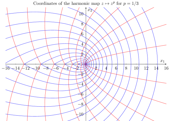
Figure 8: Change of coordinates induced by the conformal map $z\mapsto z^{p}$ for $p=1/3$. The red lines corresponds to constant values of $\bar{x}_{2}$ for $\bar{x}_{1}>\cot(p\pi)\left|\bar{x}_{2}\right|$ and the blue lines to constant values of $\bar{x}_{1}$ for $\left|\bar{x}_{2}\right|<\tan(p\pi)\bar{x}_{1}$.

The idea is now to look at large values of $\bar{x}_{1}$ with $\bar{x}_{2}$ fixed, so the scaling is as follows

$$\frac{\partial}{\partial\bar{x}_{1}} \sim\bar{x}_{1}^{-1}\,, \frac{\partial}{\partial\bar{x}_{2}} \sim 1\,,$$

and therefore if the stream function grows like $\bar{x}_{1}^{1/p-\alpha-1}$ at fixed $\bar{x}_{2}$ for some $\alpha\geq 0$, we have

$$\boldsymbol{u} \sim\begin{pmatrix}\bar{x}_{1}^{-\alpha}&\bar{x}_{1}^{-\alpha-1}\end{pmatrix}\,, \boldsymbol{\nabla}\boldsymbol{u} \sim\begin{pmatrix}\bar{x}_{1}^{-\alpha-1/p}&\bar{x}_{1}^{-\alpha-1/p-1}\\ \bar{x}_{1}^{-\alpha-1/p+1}&\bar{x}_{1}^{-\alpha-1/p}\end{pmatrix}\,,$$

in the new basis $\left\{\bar{\boldsymbol{e}}_{1},\bar{\boldsymbol{e}}_{2}\right\}$. The laplacian is

$$\Delta\boldsymbol{u}\sim\begin{pmatrix}\bar{x}_{1}^{-\alpha-2/p+2}&\bar{x}_{1}^{-\alpha-2/p+1}\end{pmatrix}\,,$$

and

$$\boldsymbol{u}\boldsymbol{\cdot}\boldsymbol{\nabla}\boldsymbol{u}\sim\begin{pmatrix}\bar{x}_{1}^{-2\alpha-1/p}&\bar{x}_{1}^{-2\alpha-1/p-1}\end{pmatrix}\,,$$

so with respect to this scaling the Navier-Stokes equations are critical for $\alpha=1/p-2$. Moreover, the decay of the pressure that is compatible is given by $p\sim\bar{x}_{1}^{-2\alpha-2}$. In these coordinates, the net force is given by

$$\boldsymbol{F}=\lim_{\bar{x}_{1}\to\infty}\int_{-\tan(p\pi)\bar{x}_{1}}^{+\tan(p\pi)\bar{x}_{1}}\mathbf{T}\boldsymbol{\cdot}\bar{\boldsymbol{e}}_{1}h\mathrm{d}\bar{x}_{2}\,.$$

The stress tensor (LABEL:stress-tensor) behaves like $\mathbf{T}\sim\bar{x}_{1}^{-2\alpha}$, so by assuming that $\mathbf{T}$ decays fast enough in $\bar{x}_{2}$, we obtain that $\boldsymbol{F}=\boldsymbol{0}$ if $\alpha>\frac{1}{2}-\frac{1}{2p}$. Therefore, the critical decay to obtain a nonzero net force is $\alpha=\frac{1}{2}-\frac{1}{2p}$ and if moreover we impose that the Navier-Stokes equations are critical, i.e. $\alpha=1/p-2$, we obtain the following result

$$\alpha =1\,, p =\frac{1}{3}\,.$$

As in the case of the homogeneous decay, we consider the following ansatz for the stream function,

$$\psi_{0}(\bar{x}_{1},\bar{x}_{2})=\bar{x}_{1}\varphi_{0}(\bar{x}_{2})\,,$$ (39)

so we have

$$\boldsymbol{u}_{0} =\frac{1}{3\left|\bar{\boldsymbol{x}}\right|^{2}}\left[-\bar{x}_{1}\varphi_{0}^{\prime}(\bar{x}_{2})\,\bar{\boldsymbol{e}}_{1}+\varphi_{0}(\bar{x}_{2})\bar{\boldsymbol{e}}_{2}\right]\,, p_{0} =\frac{\rho_{0}(\bar{x}_{2})}{\bar{x}_{1}^{4}}\,.$$ (40)

By plugging (LABEL:wake-ansatz) into the Navier-Stokes equations (LABEL:intro-ns-eq), we obtain

$$\boldsymbol{f}\boldsymbol{\cdot}\bar{\boldsymbol{e}}_{1} =\frac{1}{27\bar{x}_{1}^{5}}\left(-\varphi_{0}^{(3)}(\bar{x}_{2})+\varphi_{0}(\bar{x}_{2})\varphi_{0}^{\prime\prime}(\bar{x}_{2})+\varphi_{0}^{\prime}(\bar{x}_{2})^{2}+O(\bar{x}_{1}^{-1})\right)\,,$$

$$\boldsymbol{f}\boldsymbol{\cdot}\bar{\boldsymbol{e}}_{2} =\frac{1}{27\bar{x}_{1}^{6}}\left(-3\varphi_{0}^{\prime\prime}(\bar{x}_{2})+2\bar{x}_{2}\varphi_{0}^{\prime}(\bar{x}_{2})^{2}-\varphi_{0}(\bar{x}_{2})\varphi_{0}^{\prime}(\bar{x}_{2})-9\rho_{0}^{\prime}(\bar{x}_{2})+O(\bar{x}_{1}^{-1})\right)\,,$$

and by setting

$$\varphi_{0}(\bar{x}_{2}) =-2a\tanh(a\bar{x}_{2})\,,$$

$$\rho_{0}(\bar{x}_{2}) =\frac{4a^{2}}{27}\Big{[}4a\bar{x}_{2}\tanh(a\bar{x}_{2})-4\log\left(2\cosh(a\bar{x}_{2})\right)$$

$$\phantom{=\frac{4a^{2}}{27}\Big{[}}+\left(2a\bar{x}_{2}\tanh(a\bar{x}_{2})+7\text{sech}^{2}(a\bar{x}_{2})\right)\text{sech}(a\bar{x}_{2})\Big{]}\,,$$

where $a>0$, we obtain that (LABEL:wake-ansatz) is an exact solution of the Navier-Stokes equations in $D$ with some $\boldsymbol{f}=O(\bar{x}_{1}^{-6})\bar{\boldsymbol{e}}_{1}+O(\bar{x}_{1}^{-7})\bar{\boldsymbol{e}}_{2}=\left(O(r^{-6/3}),O(r^{-7/3})\right)$. By an explicit calculation, the stress tensor including the convective term is

$$\mathbf{T}_{0}=\frac{-\varphi_{0}^{\prime}(\bar{x}_{2})^{2}}{9\bar{x}_{1}^{2}}\bar{\boldsymbol{e}}_{1}\otimes\bar{\boldsymbol{e}}_{1}+O(\bar{x}_{1}^{-3})\,,$$

so the net force is then given by

$$\boldsymbol{F}=\lim_{\bar{x}_{1}\to\infty}\int_{-\tan(p\pi)\bar{x}_{1}}^{+\tan(p\pi)\bar{x}_{1}}\mathbf{T}\boldsymbol{\cdot}\bar{\boldsymbol{e}}_{1}h\mathrm{d}\bar{x}_{2}=\int_{-\infty}^{+\infty}\left(\frac{-1}{3}\varphi_{0}^{\prime}(\bar{x}_{2})^{2},0\right)=\left(-\frac{16a^{3}}{9},0\right)\,.$$

However, the stream function (LABEL:wake-psi0) when expressed back in the coordinates $(x_{1},x_{2})$ is not continuous along the line $\left\{(x_{1},0)\,,x_{1}<0\right\}$, there is a jump of order $O(\left|x_{1}\right|^{1/3})$. This jump will be removed at the next order.

The role of the next order is to improve the decay of the remainder $\boldsymbol{f}$, so we make the Ansatz,

$$\psi_{1}(\bar{x}_{1},\bar{x}_{2})=\varphi_{1}(\bar{x}_{2})\,,$$

in order to cancel the term decaying like $O(\bar{x}_{1}^{-6})\bar{\boldsymbol{e}}_{1}+O(\bar{x}_{1}^{-7})\bar{\boldsymbol{e}}_{2}$ in the remainder of the previous order. We have

$$\boldsymbol{u}_{1} =\frac{-1}{3\left|\bar{\boldsymbol{x}}\right|^{2}}\varphi_{1}^{\prime}(\bar{x}_{2})\,\bar{\boldsymbol{e}}_{1}\,, p_{1} =\frac{\rho_{1}(\bar{x}_{2})}{\bar{x}_{1}^{5}}\,.$$

By plugging $\boldsymbol{u}=\boldsymbol{u}_{0}+\boldsymbol{u}_{1}$ and $p=p_{0}+p_{1}$ into the Navier-Stokes equations (LABEL:intro-ns-eq), we obtain

$$\boldsymbol{f}\boldsymbol{\cdot}\bar{\boldsymbol{e}}_{1} =\frac{1}{27\bar{x}_{1}^{6}}\left(-\varphi_{1}^{(3)}(\bar{x}_{2})+\varphi_{0}(\bar{x}_{2})\varphi_{1}^{\prime\prime}(\bar{x}_{2})+3\varphi_{0}^{\prime}(\bar{x}_{2})\varphi_{1}^{\prime}(\bar{x}_{2})+O(\bar{x}_{1}^{-1})\right)\,,$$

$$\boldsymbol{f}\boldsymbol{\cdot}\bar{\boldsymbol{e}}_{2} =\frac{1}{27\bar{x}_{1}^{6}}\left(-4\varphi_{1}^{\prime\prime}(\bar{x}_{2})+4\bar{x}_{2}\varphi_{0}^{\prime}(\bar{x}_{2})\varphi_{1}^{\prime}(\bar{x}_{2})-9\rho_{1}^{\prime}(\bar{x}_{2})+O(\bar{x}_{1}^{-1})\right)\,.$$

So by setting

$$\varphi_{1}(\bar{x}_{2}) =\sqrt{3}\left(\frac{2a\bar{x}_{2}}{3}-\tanh(a\bar{x}_{2})-a\bar{x}_{2}\operatorname{sech}^{2}(a\bar{x}_{2})\right)\,,$$

$$\rho_{1}(\bar{x}_{2}) =\frac{2\sqrt{3}a}{27}\operatorname{sech}^{4}(a\bar{x}_{2})\left(6a^{2}\bar{x}_{2}^{2}-4az\sinh(2a\bar{x}_{2})+7\cosh(2a\bar{x}_{2})+7\right)\,,$$

we obtain that $\boldsymbol{u}=\boldsymbol{u}_{0}+\boldsymbol{u}_{1}$ and $p=p_{0}+p_{1}$ is an exact solution of the Navier-Stokes equations (LABEL:intro-ns) in $D$ with some $\boldsymbol{f}=O(\bar{x}_{1}^{-7})\bar{\boldsymbol{e}}_{1}+O(\bar{x}_{1}^{-8})\bar{\boldsymbol{e}}_{2}=\left(O(r^{-7/3}),O(r^{-8/3})\right)$. Moreover, the jump in the stream function $\psi=\psi_{0}+\psi_{1}$ on the line $\left\{(x_{1},0)\,,x_{1}<0\right\}$ is now uniformly bounded.

Therefore, we obtained the following result:

Proposition 5.1.

For any $\boldsymbol{F}\neq 0$, there exists a solution $({\boldsymbol{U}\!}_{\boldsymbol{F}},P_{\boldsymbol{F}})\in C^{\infty}(\mathbb{R}^{2})$ with some $\boldsymbol{f}\in C^{\infty}(\mathbb{R}^{2})$ of the Navier-Stokes equations in $\mathbb{R}^{2}$ with ${\boldsymbol{U}\!}_{\boldsymbol{F}}=O(\left|\boldsymbol{x}\right|^{-1/3})$, $P_{\boldsymbol{F}}=O(\left|\boldsymbol{x}\right|^{-2/3})$ and $\boldsymbol{f}=\left(O(\left|\boldsymbol{x}\right|^{-7/3}),O(\left|\boldsymbol{x}\right|^{-8/3})\right)$.

Proof.

By adding the term $\frac{3\sqrt{3}}{\pi}\arg(\bar{x}_{1}+\mathrm{i}\bar{x}_{2})$ to the stream function $\psi_{0}+\psi_{1}$ and also terms decaying faster at infinity, we can construct a smooth stream function $\psi$ which generates a solution $({\boldsymbol{U}\!}_{\boldsymbol{F}},P_{\boldsymbol{F}})\in C^{\infty}(\mathbb{R}^{2})$ of Navier-Stokes equations (LABEL:intro-ns) in $\mathbb{R}^{2}$ with ${\boldsymbol{U}\!}_{\boldsymbol{F}}=O(\left|\boldsymbol{x}\right|^{-1/3})$, $P_{\boldsymbol{F}}=O(\left|\boldsymbol{x}\right|^{-2/3})$ and some $\boldsymbol{f}=\left(O(r^{-7/3}),O(r^{-8/3})\right)$ such that $\boldsymbol{F}=\left(-\frac{16a^{3}}{9},0\right)$. Since the equations are rotational invariant, we can rotate this solution to obtain any $\boldsymbol{F}\neq\boldsymbol{0}$. ∎

The solution $({\boldsymbol{U}\!}_{\boldsymbol{F}},P_{\boldsymbol{F}})$ is represented in wake-ansatz for $\boldsymbol{F}=(-F,0)$ with some $F>0$. Within a wake the velocity field decays like $\left|\boldsymbol{x}\right|^{-1/3}$ whereas outside the wake it decays like $\left|\boldsymbol{x}\right|^{-2/3}$. The width of the wake is decreasing as the net force is increasing. Moreover, we believe that this solution describes the general asymptote of any solutions with small enough $\boldsymbol{f}$ or $\boldsymbol{u}^{*}$ having a nonzero net force $\boldsymbol{F}\neq\boldsymbol{0}$:

Conjecture 5.2.

For a large class of boundary conditions $\boldsymbol{u}^{*}$ and source terms $\boldsymbol{f}$ with a nonzero net force $\boldsymbol{F}$, there exists a solution to (LABEL:intro-ns) with $\boldsymbol{u}_{\infty}=\boldsymbol{0}$ which satisfies

$$\boldsymbol{u} ={\boldsymbol{U}\!}_{\boldsymbol{F}}+O(r^{-1})\,, p =P_{\boldsymbol{F}}+O(r^{-2})\,,$$

where $\left({\boldsymbol{U}\!}_{\boldsymbol{F}},P_{\boldsymbol{F}}\right)$ is the solution constructed in wake-UF-PF.

Once the asymptotic behavior is determined, the idea to prove its validity is to lift the compatibility conditions by using the asymptotic behavior, as the Landau solution does in three dimensions. However, due to the decay in $\left|\boldsymbol{x}\right|^{-1/3}$ of the asymptote, instead of (LABEL:compatibility-ns-landau), we have to consider the linear problem

$$\Delta\boldsymbol{v}-\boldsymbol{\nabla}q-{\boldsymbol{U}\!}_{\boldsymbol{F}}\boldsymbol{\cdot}\boldsymbol{\nabla}\boldsymbol{v}-\boldsymbol{v}\boldsymbol{\cdot}\boldsymbol{\nabla}{\boldsymbol{U}\!}_{\boldsymbol{F}} =\boldsymbol{g}\,, \boldsymbol{\nabla}\boldsymbol{\cdot} \boldsymbol{u}=0\,,$$

where $\boldsymbol{g}$ is a given source term. To our knowledge, this linear problem is not solvable with the mathematical methods developed so far. The reason is the following: in view of the regularity, one has to inverse the whole Laplacian $\Delta$, which is the operator of highest degree, otherwise we loose regularity and in view of the decay at infinity, one has to inverse

$$\left(\boldsymbol{F}\boldsymbol{\cdot}\boldsymbol{\nabla}\right)^{2}\boldsymbol{v}-{\boldsymbol{U}\!}_{\boldsymbol{F}}\boldsymbol{\cdot}\boldsymbol{\nabla}\boldsymbol{v}-\left(\boldsymbol{v}\boldsymbol{\cdot}\boldsymbol{F}\right)\,\boldsymbol{F}\boldsymbol{\cdot}\boldsymbol{\nabla}{\boldsymbol{U}\!}_{\boldsymbol{F}}\,,$$

which leads to regularity lost in the direction $\boldsymbol{F}^{\perp}$. Therefore, in order to solve this linear problem, one has to face with these two opposing principles. This will be part of further investigations. However, the validity of the conjecture as well as the other asymptotic regimes for the case of a vanishing net force will be investigated numerically in the next sections.

Figure 9: Velocity field ${\boldsymbol{U}\!}_{\boldsymbol{F}}$ of wake-UF-PF for $\boldsymbol{F}=(-F,0)$ with different values of $F>0$. The color represent the magnitude of $\left|\boldsymbol{x}\right|^{1/3}{\boldsymbol{U}\!}_{\boldsymbol{F}}$ in order to highlight, the fact the ${\boldsymbol{U}\!}_{\boldsymbol{F}}$ decays like $\left|\boldsymbol{x}\right|^{-1/3}$ inside a wake and like $\left|\boldsymbol{x}\right|^{-2/3}$ outside.

22 Numerical simulations with Stokes solutions as boundary conditions

In an attempt to determine the general asymptotic behavior numerically, we consider the Navier-Stokes equations (LABEL:intro-ns) in the domain $\Omega=\mathbb{R}^{2}\setminus\macc@depth\char 1\relax\frozen@everymath{\macc@group}\macc@set@skewchar\macc@nested@a 111{B}$ where $B=B(\boldsymbol{0},1)$. In view of failure-asymptotic and strong-under-compatibility, we have seen that the problematic solutions of the Stokes equations in order to construct a solutions of the Navier-Stokes equations are the asymptotic term $\boldsymbol{S}_{0}$ and $\boldsymbol{S}_{1}$ given in lin-stokes-asy. Therefore, the idea is to take for the boundary condition on $\partial B$, the evaluation of the problematic asymptotic terms,

$$\boldsymbol{u}^{*}=\left.\boldsymbol{S}_{0}+\boldsymbol{S}_{1}\right|_{\partial B}=\boldsymbol{C}_{0}\boldsymbol{\cdot}\mathbf{E}_{0}+\boldsymbol{C}_{1}\boldsymbol{\cdot}\mathbf{E}_{1}\,,$$

where $\boldsymbol{C}_{0}\in\mathbb{R}^{2}$ and $\boldsymbol{C}_{1}\in\mathbb{R}^{3}$ are parameters. Explicitly, by using lin-stokes-asy, we have

$$\boldsymbol{u}^{*}=\frac{-1}{4\pi}\left[\boldsymbol{C}_{0}\boldsymbol{\cdot}\left(\cos\theta,\sin\theta\right)\,\boldsymbol{e}_{r}+\boldsymbol{C}_{1}\boldsymbol{\cdot}\left(\cos(2\theta)\boldsymbol{e}_{r},\sin(2\theta)\boldsymbol{e}_{r},\boldsymbol{e}_{\theta}\right)\right]\,.$$ (41)

The different boundary conditions are represented in plot-bc. Trivially the solution of the Stokes equations (LABEL:compatibility-stokes) satisfying this boundary condition grows at infinity like $\log\left|\boldsymbol{x}\right|$ unless $\boldsymbol{C}_{0}=\boldsymbol{0}$. We will see numerically that the solution of the Navier-Stokes equations subject to the same boundary condition will decay like $\left|\boldsymbol{x}\right|^{-1/3}$ or faster. In order to simulate this problem, we truncate the domain $\Omega$ to a ball $B(\boldsymbol{0},R)$ of radius $R=10^{5}$, and put open boundary conditions on the artificial boundary $\partial B(\boldsymbol{0},R)$. We make simulations for various choices of the parameters $\boldsymbol{C}_{0}$ and $\boldsymbol{C}_{1}$. In order to systematically analyze the solutions, we determine numerically for each value of the parameters, the functions

$$d(r) =\max_{\theta\in[-\pi,\pi]}\left|\boldsymbol{u}(r,\theta)\right|\,, a(r) =\operatorname*{arg\,max}_{\theta\in[-\pi,\pi]}\left|\boldsymbol{u}(r,\theta)\right|\,.$$ (42)

In view of the symmetry of the boundary condition a nonzero net force can be generated only if $\boldsymbol{C}_{0}\neq\boldsymbol{0}$.

Figure 10: Representation of the vector field $\boldsymbol{u}^{*}$ given by (LABEL:plot-bc) with $\boldsymbol{C}_{1}=\boldsymbol{0}$ for the first line and $\boldsymbol{C}_{0}=\boldsymbol{0}$ for the second one.

22.1 Nonzero net force

First, we consider the case $\boldsymbol{C}_{0}\neq\boldsymbol{0}$ which might generate a nonzero net force. Without lost of generality, we can perform a rotation such that $\boldsymbol{C}_{0}=\left(-\mathcal{F},0\right)$ with $\mathcal{F}>0$. In order to keep only two free parameters, we choose $\boldsymbol{C}_{1}=\left(0,0,-\mathcal{M}\right)$ with $\mathcal{M}>0$. We perform simulations for $\mathcal{F}\in\left\{0,0.08,0.16,\dots,18\right\}\pi$ and $\mathcal{M}\in\left\{0,0.08,0.16,\dots,36\right\}\pi$. Since the problem is highly nonlinear, we used a parametric solver in order to follow the evolution of the solution starting from $\mathcal{F}=\mathcal{M}=0$. Even with this parametric solver, the nonlinear solver fails to converge for $\mathcal{F}\geq 8\pi$ and $\mathcal{M}\leq 28\pi$ approximately; more precisely on the blank region of plot-Fmu.

The velocity magnitude is represented in sim-Fmu-5,sim-Fmu-20 respectively on the line $\mathcal{F}=2\pi$ and $\mathcal{F}=8\pi$ for varying values of $\mathcal{A}$. At $\mathcal{A}=0$, the velocity field presents a wake behavior with a decay like $r^{-1/3}$ along the first axis. The opening of the wake depends on $\mathcal{F}$. As $\mathcal{A}$ is increasing, the orientation of the wake in varying and when $\mathcal{A}$ is big enough, the wake behavior becomes blurred and the solution has an homogeneous decay like $r^{-1}$. It is an interesting result, that we observe a kind of phase transition between a decay like $r^{-1/3}$ and a decay like $r^{-1}$. This is expected, since for $\mathcal{M}>16\sqrt{3}\pi$ and $\mathcal{F}$ small enough, Hillairet & Wittwer (2013) proved that the asymptote is given by $\mu\boldsymbol{e}_{\theta}/r$ for some $\mu>0$.

We then make a more systematic analysis. In the region characterized by $3\times 10^{2}\leq r\leq 3\times 10^{4}$, the function $d$ seems to be already in the asymptotic regime and not influenced by the artificial boundary condition. We use this region to determine the power of decay of the function $d$, which is represented in plot-Fmua in terms of $\mathcal{F}$ and $\mathcal{M}$. We then analyze the function $a$, by showing in plot-Fmub its mean value over $3\times 10^{2}\leq r\leq 3\times 10^{4}$. In order to determine if this mean value is accurate or not, we compute the standard deviation of $a$ and represent large standard deviations as more transparent colors. At fixed value of $\mathcal{F}$ the angle is increasing with $\mathcal{M}$ until the power of decay becomes almost $r^{-1}$. We compute the net force and net torque acting on the body,

$$\boldsymbol{F} =\int_{\partial B}\mathbf{T}\boldsymbol{n}\,, M =\int_{\partial B}\boldsymbol{x}\boldsymbol{\wedge}\mathbf{T}\boldsymbol{n}\,.$$

The magnitude of the net force $\boldsymbol{F}$ is shown in plot-Fmuc and its angle in plot-Fmud. If the net force is too small, the angle is ill-defined, so we add more transparency to smallest net forces. As expected the net force is zero in the region where the power of decay is $r^{-1}$ and is increasing with $\mathcal{F}$ in the other region. In plot-Fmue, we represent the net torque $M$ which increases almost linearly as a function of $\mathcal{M}$ and is independent of $\mathcal{F}$. Finally, in plot-Fmuf, we represent the difference between the angle of the net force and the angle corresponding to the slowest decay. The two angles almost coincide in the region where the angles are well-defined, i.e. when the net force is not too small and when the power of decay is $r^{-1/3}$.

Moreover, one can show (see Guillod & Wittwer, 2015a) that the numerical solutions verify wake-conj, i.e. its asymptotic behavior is given by ${\boldsymbol{U}\!}_{\boldsymbol{F}}$.

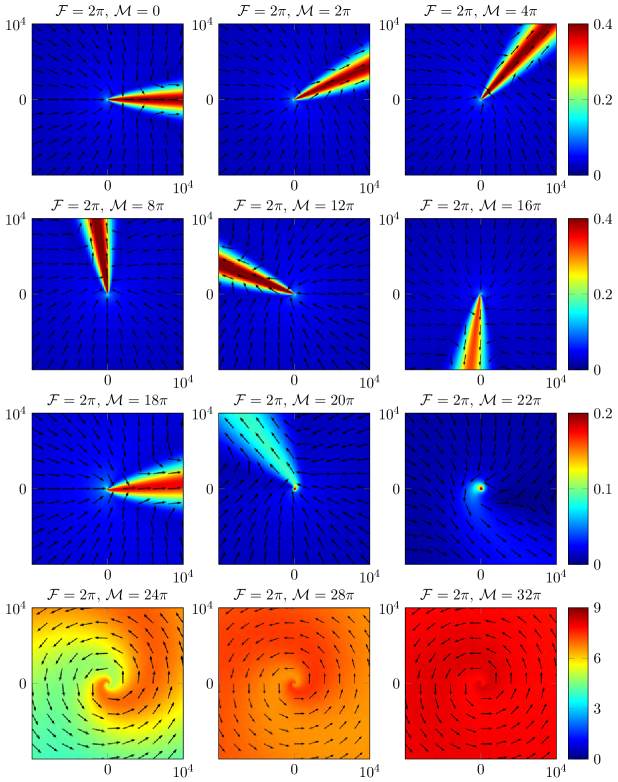
Figure 11: Numerical simulations on the line $\mathcal{F}=2\pi$ of the velocity magnitude multiplied by $r^{1/3}$ for the first three lines and by $r$ for the last one.

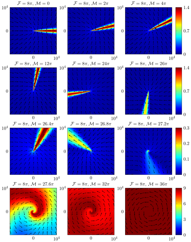
Figure 12: Numerical simulations on the line $\mathcal{F}=8\pi$ of the velocity magnitude multiplied by $r^{1/3}$ for the first three lines and by $r$ for the last one.

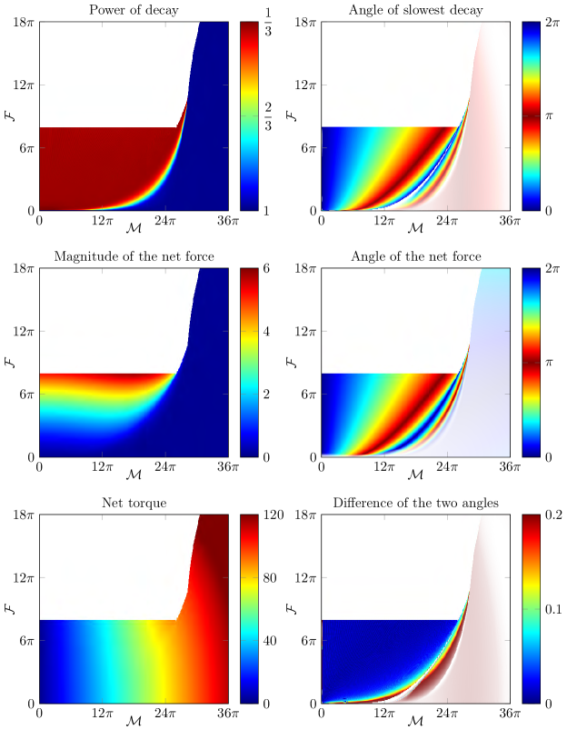
Figure 13: Main characteristics of the solution for varying $\mathcal{F}$ and $\mathcal{M}$: (a) the power of decay of the function $d$; (b) the mean of the function $a$ with its standard deviation shown with transparency; (c) the magnitude of the net force acting on the body $B$; (d) the angle of the net force with the magnitude of the net force in transparency; (e) the net torque acting on the body; (f) the difference between the angle drawn on (b) and (d).

22.2 Zero net force

Second, we consider the case where $\boldsymbol{C}_{0}=\boldsymbol{0}$, for which we know by symmetry that the net force is zero. By a rotation and a reflection, we can without generality assume that $\boldsymbol{C}_{1}=\left(-\mathcal{A},0,-\mathcal{M}\right)$, with $\mathcal{A},\mathcal{M}\geq 0$. We perform numerical simulations for $\mathcal{A}\in\left\{0,0.4,0.8,\dots,36\right\}\pi$ and $\mathcal{M}\in\left\{0,0.4,0.8,\dots,36\right\}\pi$. Again, for values far from $\mathcal{A}=\mathcal{F}=0$, the nonlinear solver has difficulties do converge, so we use a parametric solver to follow the solution. At fixed value of $\mathcal{M}$, we perform a parametric continuation from $\mathcal{F}=0$ to $\mathcal{F}=36\pi$, as shown in plot-parametrica, or we do the converse as shown in plot-parametricb and surprisingly the results are not the same.

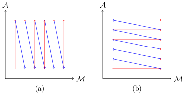
Figure 14: In order to study the dependence of the solution on two parameters $\mathcal{A}$ and $\mathcal{F}$, we have two choices: (a) at fixed value of $\mathcal{M}$ we perform a parametric continuation on $\mathcal{A}$ or (b) at fixed value of $\mathcal{F}$ we use a parametric solver in $\mathcal{M}$.

The magnitude of the velocity $\boldsymbol{u}$ on the line $\mathcal{A}=8\pi$ for varying $\mathcal{M}$ is shown in sim-Amu-20. For such small values of $\mathcal{A}$, we are at small Reynolds number, so this is not clear if the computational domain is big enough for seeing the real asymptotic behavior and not only the Stokes one. Therefore, we cannot conclude that the velocity decays like $r^{-1}$ or like $r^{-1/3}$. On the line $\mathcal{A}=18\pi$ (sim-Amu-45), the velocity decay like $r^{-1/3}$ for small values of $\mathcal{M}$ and like $r^{-1}$ for large ones, so the first two lines of the figure, the velocity magnitude is multiplied by $r^{1/3}$ and on the last two by $r$. At $\mathcal{M}=0$, we have a double wake characterized by ${\boldsymbol{U}\!}_{\boldsymbol{F}}+{\boldsymbol{U}\!}_{-\boldsymbol{F}}$ for some $\boldsymbol{F}=(-F,0)$ depending on $\mathcal{A}$ and this double wake is rotated by an increasing angle in term of $\mathcal{M}$. Around $\mathcal{M}=8.8\pi$, the wake behavior disappears and the solution is asymptotic to the harmonic solution $\mu\boldsymbol{e}_{\theta}/r$ for some $\mu\in\mathbb{R}$. On the last line of sim-Amu-45 we represent the norm $r\left|\boldsymbol{u}-\mu\boldsymbol{e}_{\theta}/r\right|$ for the best $\mu\in\mathbb{R}$. The same analysis is done in sim-Amu-90 for $\mathcal{A}=36\pi$. Near $\mathcal{A}=\mathcal{F}=16\pi$, the solution depends on the way we approach it: either the velocity decays like $r^{-1/3}$ either like $r^{-1}$. We note that sim-Amu-45f is similar to the spiral solutions found in Guillod & Wittwer (2015b) with $n=2$.

In the same way, we also analyze the functions (LABEL:functions-d-a). The power of decay in both cases are respectively shown in plot-Amua and plot-Amuc. In this situation the slowest decay is given by two angles separated by $\pi$, so we take the mean of the function $a$ modulo $\pi$, as shown in plot-Amub and plot-Amud. Surprisingly, the two ways we used the parametric solver do not produce the same results in a small triangle near $\mathcal{A}=\mathcal{F}=16\pi$. Especially the power of decay seems to be $r^{-1/3}$ when the value of $\mathcal{A}$ is increasing and like $r^{-1}$ when the value of $\mathcal{M}$ is increasing. This strange behavior may either mean that the solution is not unique or that the precision of the numerical solver in not good enough to discard one of the two solutions.

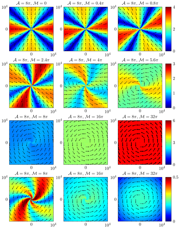
Figure 15: Numerical simulations on the line $\mathcal{A}=8\pi$ of the velocity magnitude multiplied by $r$ for the first three lines. Since $\mathcal{A}$ is small, for small values of $\mathcal{M}$ the velocity behaves like the solution of the Stokes equations except that the velocity is bigger in the outflow regions than in the inflow regions. For $\mathcal{M}$ larger than approximately $8\pi$, the velocity is close to the harmonic solution $\mu\boldsymbol{e}_{\theta}/r$ for some $\mu\in\mathbb{R}$. In the last line we represent the magnitude $\left|r\boldsymbol{u}-\mu\boldsymbol{e}_{\theta}\right|$ of the optimal $\mu$ that minimize the remainder.

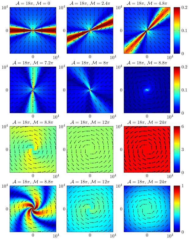
Figure 16: Numerical simulations for $\mathcal{A}=18\pi$. The first two lines represent $r^{1/3}\left|\boldsymbol{u}\right|$, the third one $r\left|\boldsymbol{u}\right|$ and the last one $\left|r\boldsymbol{u}-\mu\boldsymbol{e}_{\theta}\right|$ for the best $\mu$. For small $\mathcal{M}$, the velocity is well-modeled by the solution ${\boldsymbol{U}\!}_{\boldsymbol{F}}$ of wake-UF-PF. As $\mathcal{M}$ increases, the double wake rotates, its magnitude decreases and disappears around $\mathcal{M}=8.8\pi$. From this value the the velocity is close to the exact solution $\mu\boldsymbol{e}_{\theta}/r$ for some $\mu\in\mathbb{R}$.

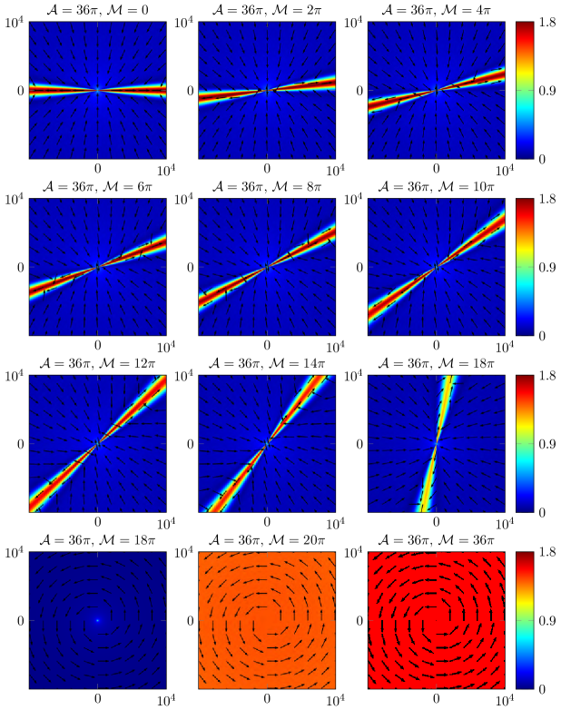
Figure 17: Numerical simulations for $\mathcal{A}=36\pi$. The first three lines represent $r^{1/3}\left|\boldsymbol{u}\right|$ and the last one $r\left|\boldsymbol{u}\right|$. As $\mathcal{A}$ is bigger than in sim-Amu-45, the opening of the double wake is more narrow, so it corresponds to ${\boldsymbol{U}\!}_{\boldsymbol{F}}+{\boldsymbol{U}\!}_{-\boldsymbol{F}}$ with a bigger value of $\left|\boldsymbol{F}\right|$. As $\mathcal{M}$ increases, the magnitude of the double wake is reduced and finally the velocity decays like $r^{-1}$ for large values of $\mathcal{M}$.

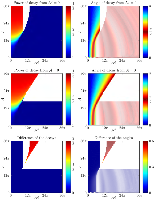
Figure 18: Main characteristics of the numerical solution for varying $\mathcal{A}$ and $\mathcal{M}$. The power of decay of the function $d$ when the parametric solver is used at fixed value of $\mathcal{M}$ or $\mathcal{A}$ is drawn in (a) and (c) respectively, its difference is (e). The angle of the slowest decay which is the mean of the function $a$ with its standard deviation shown with transparency is represented on (b) and (d) respectively for the parametric solver used at fixed value of $\mathcal{M}$ or $\mathcal{A}$ and the difference is (f).

23 Numerical simulations with multiple wakes

Figure 19: Representation of the force (LABEL:delta-n-f), which is $n$ approximations of the delta-function uniformly distributed on the circle on radius five.

Finally, we examine the possibility of generating more than one or two wakes. The idea is to take $\boldsymbol{f}$ having $n$ approximations of the delta function distributed on the circle of radius five (see delta-n-forces),

$$\boldsymbol{f}(\boldsymbol{x})=-\mathcal{A}\sum_{i=0}^{n-1}\delta_{\varepsilon}(\boldsymbol{x}-5\mathbf{R}_{2\pi i/n}\boldsymbol{e}_{1})\mathbf{R}_{2\pi i/n}\boldsymbol{e}_{1}\,,$$ (43)

where $\mathcal{A}\in\mathbb{R}$ is an amplitude, $\mathbf{R}_{\vartheta}\in\mathrm{SO}(2)$ is the rotation matrix of angle $\vartheta$, and $\delta_{\varepsilon}$ is the following approximation of the $\delta$-function,

$$\delta_{\varepsilon}(\boldsymbol{x})=\frac{1}{\pi\varepsilon}\mathrm{e}^{-\left|\boldsymbol{x}\right|^{2}/\varepsilon}\,.$$

We perform numerical simulations in a disk $B(\boldsymbol{0},R)$ of radius $R=10^{4}$ with open boundary conditions on $\partial B(\boldsymbol{0},R)$ and $\varepsilon=0.1$, which leads to the results drawn in branches-u. For $n=1$, we recover the straight simple wake studied in details in asy-wake. For $n=2$, we obtain two wakes which are in opposite directions so that the net is effectively zero. For small values of $\mathcal{A}$, the solution is very close to the solution of the Stokes equations on a huge domain, so the magnitude of velocity is quasi similar along the first and second axes, and decay like $r^{-1}$ on the computational domain. As $\mathcal{A}$ increases, this property is more and more destroyed with the emergence of the two wakes that decay like $r^{-1/3}$. For $n=3$, the situation is similar. For $n=4$, for small values of $\mathcal{A}$, the velocity decays almost like $r^{-2}$, but as $\mathcal{A}$ increases this situation becomes unstable, and around $\mathcal{A}=96$, two wakes with an angle of $\frac{\pi}{4}$ and $\frac{5\pi}{4}$ are created. By symmetry, the same solution rotated by $\frac{\pi}{2}$ is also a solution, so the choice between the two possibilities comes from the symmetry breaking due to the meshing of the domain. As $\mathcal{A}$ increases even more, the two wakes separate to become four distinct wakes.

Finally, we determine in branches-decay the power of decay of $\left|\boldsymbol{u}\right|$ inside the wake on the region $10^{2}\leq r\leq 8\times 10^{3}$ in which the magnitude of the velocity seems to have a constant power of decay not influenced by the artificial boundary conditions. For $n=1$, the power of decay is essentially $r^{-1/3}$ as shown in wake-sim, except for small values of $\mathcal{A}$ for which the computational domain is too small. For $n=2$, almost the same situation appears: for small value of $\mathcal{A}$ the solution is close to the Stokes solution which decays like $r^{-1}$ in a large domain, so for small value of $\mathcal{A}$ the apparent decay of the numerical solution is almost $r^{-1}$. For larger $\mathcal{A}$, the two wakes decay like $r^{-1/3}$ and the velocity fields are almost fitted by ${\boldsymbol{U}\!}_{\boldsymbol{F}}+{\boldsymbol{U}\!}_{-\boldsymbol{F}}$ where $\boldsymbol{F}$ depends on $\mathcal{A}$. For $n=3$, the solution of the Stokes equations decay like $r^{-2}$ and therefore, for small values of $\mathcal{A}$ the power of decay inside the computational domain is near $r^{-2}$. As $\mathcal{A}$ increases, the three wakes described by some ${\boldsymbol{U}\!}_{\boldsymbol{F}}$ emerge and decay almost like $r^{-1/3}$. For $n=4$, there is a regime with two wakes that break the symmetry before splitting into four wakes. The power of decay in branches-u seems to indicate that at small Reynolds numbers, only one or two wakes can exist and that an higher number of wakes is present only at large Reynolds numbers.

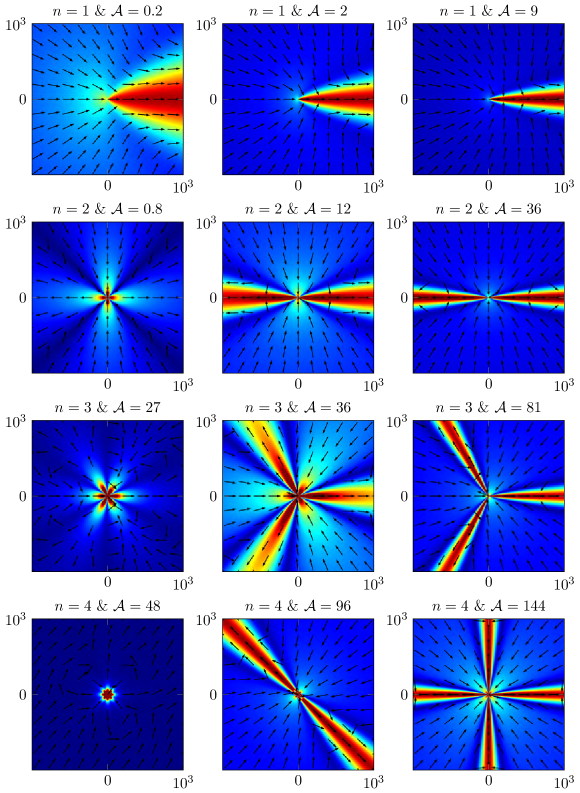
Figure 20: Magnitude for the velocity field $r^{1/3}\left|\boldsymbol{u}\right|$ obtained by numerical simulations with $n$ approximations of the delta function for the source force (LABEL:delta-n-f). For small value of the amplitude $\mathcal{A}$, the solution is close to the solution of the Stokes equations on a large domain, but for large data, we obtain $n$ wakes. For $n=4$ and $\mathcal{A}=96$, the numerically found solution breaks the symmetry of the source force.

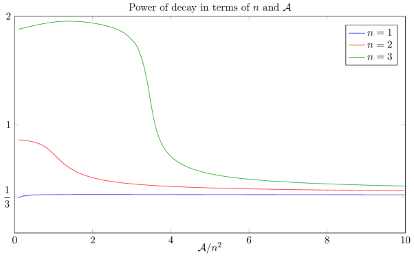
Figure 21: Power of decay of the numerical solutions fitted in the region $10^{2}\leq r\leq 8\times 10^{3}$. For small values of $\mathcal{A}$, the velocity decays like the solution of the Stokes equations in a large region which explains the behavior of the power of decay near $\mathcal{M}=0$. For large values of $\mathcal{M}$ the velocity behaves like $r^{-1/3}$.

24 Conclusions

If the net force is nonzero, we have a physically motivated conjecture for the asymptotic behavior of the solution, which is verified numerically. In this case, the asymptote is given by ${\boldsymbol{U}\!}_{\boldsymbol{F}}$ which is decaying like $|\boldsymbol{x}|^{-1/3}$ inside a wake in the direction of $\boldsymbol{F}$ and like $|\boldsymbol{x}|^{-2/3}$ outside. If the net force vanishes, the velocity can be asymptotic to the double wake ${\boldsymbol{U}\!}_{\boldsymbol{F}}+{\boldsymbol{U}\!}_{-\boldsymbol{F}}$ for some $\boldsymbol{F}\in\mathbb{R}^{2}$ which also have a supercritical decay like $|\boldsymbol{x}|^{-1/3}$ . In another regime, the solution is asymptotic to the exact harmonic solution $\mu\boldsymbol{e}_{\theta}/r$, where $\mu$ is a parameter. The previous section seems to indicate that at small Reynolds number, three wakes or more are not possible. We remark that these two regimes are clearly not the only ones. By choosing particular boundary conditions on the disk, we can easily construct an exact solution that is equal at large distances to spiral solutions found in Guillod & Wittwer (2015b) for $n=2$ and arbitrary small $\kappa$. The results concerning the decay of the solutions of the Navier-Stokes equations and their asymptotic behavior are summarized is the following table:

In particular, we see that the nonlinearity of the Navier-Stokes equations seems to allow the existence of solutions decaying to zero at infinity even if the net force is nonzero, which removes the Stokes paradox that is present at the linear level.

Index

• Admissible boundary condition Definition 2.10
• Admissible domain Definition 2.9
• Asymptotic behavior
  • Navier-Stokes solutions
    • under compatibility conditions Theorem 3.6
    • under symmetries Corollary 3.7
    • weak solutions §9
  • Stokes solutions Lemma 3.2
• Asymptotic expansion
  • Navier-Stokes solutions
    • for $\boldsymbol{F}=\boldsymbol{0}$ §24
    • for $\boldsymbol{F}\neq\boldsymbol{0}$ §21
    • summary §24
  • Stokes equations Lemma 3.2, Lemma 3.3
• Axial symmetry item (b)
• Boundary condition 3
  • admissible Definition 2.10
• Central symmetry item (a)
• Compatibility conditions
  • lift by using an exact solution §15
  • Navier-Stokes equations Theorem 3.6
  • Stokes equations Lemma 3.3
• Criticality of the Navier-Stokes equations Chapter 1
• Delta-function approximation §23
• Domain
  • admissible Definition 2.9
  • exterior item 2
  • type Chapter 1
• Exact solutions
  • Euler equations §20
  • harmonic Chapter 4
  • Landau Chapter 1
  • scale-invariant solution up to a rotation Chapter 1
• Existence
  • extension §5
  • strong solutions
    • under compatibility conditions Theorem 3.6
    • under symmetries Corollary 3.7
  • weak solutions Theorem 2.15
• Extension
  • condition §5
  • existence §5
• Exterior domain item 2
• Flux Proposition 1.4
• Flux carrier §16
• Fundamental solution
  • Stokes equations §11
• Hardy inequality
  • in three dimensions Lemma 2.19
  • in two dimensions Lemma 2.20
• Inequality
  • Hardy
    • in three dimensions Lemma 2.19
    • in two dimensions Lemma 2.20
  • Poincaré Lemma 2.4
• Infinitesimal symmetry Proposition 1.1
• Invariant quantity Definition 1.2
  • net flux Proposition 1.4
  • net force Proposition 1.4
  • net torque Proposition 1.4
• Landau solutions Chapter 1
• Lift of compatibility conditions §15
• Limit of the velocity §8.1, §8.2
• Lipschitz domain Definition 2.1
• Navier-Stokes equations Chapter 1
  • asymptotic behavior
    • for $\boldsymbol{u}_{\infty}=\boldsymbol{0}$ Theorem 3.6, Corollary 3.7
  • asymptotic expansion
    • for $\boldsymbol{F}=\boldsymbol{0}$ §24
    • for $\boldsymbol{F}\neq\boldsymbol{0}$ §21
    • summary §24
  • criticality Chapter 1
  • existence of strong solutions
    • under compatibility conditions Theorem 3.6
    • under symmetries Corollary 3.7
  • limit of the velocity §8.1, §8.2
  • regularity §7
  • weak solutions Definition 2.13, Theorem 2.15
• Net flux Proposition 1.4
• Net force Proposition 1.4
  • implications on the asymptotic behavior Chapter 1
• Net torque Proposition 1.4
• Notations §1
• Numerical simulations
  • double straight wake §22
  • multiple wakes §23
  • with Stokes boundary conditions §22
• Oseen equations Chapter 1
• Paradox of Stokes Chapter 1
• Poincaré inequality Lemma 2.4
• Power counting Chapter 1
• Pressure field Chapter 1
• Regularity of weak solutions §7
• Rotational symmetry item 2
• Scale-invariant solutions Chapter 1
• Scaling
  • Navier-Stokes equations Chapter 1
  • symmetry Chapter 1, item 3
• Sobolev space Definition 2.2
• Space
  • $\mathcal{B}_{k,q}$ Definition 3.1
  • $C_{0,\sigma}^{\infty}$ Chapter 2
  • $D^{1,2}$ Definition 2.2
  • $D_{0}^{1,2}$ Definition 2.3
  • $D_{0,\sigma}^{1,2}$ Definition 2.7
  • $W^{1,2}$ Definition 2.2
  • $W_{0}^{1,2}$ Definition 2.3
• Stokes equations Chapter 1, §10
  • asymptotic behavior Lemma 3.2
  • fundamental solution §11
• Stokes paradox Chapter 1
• Stress tensor Chapter 1
• Strong solutions
  • under compatibility conditions Theorem 3.6
  • under symmetries Corollary 3.7
• Symmetry
  • axial item (b)
  • central item (a)
  • compatibility conditions §13
  • Navier-Stokes equations §2
  • rotations item 2
  • scaling Chapter 1, item 3
  • translations item 1
• Torque Proposition 1.4
• Translational symmetry item 1
• Truncation procedure §16
• Velocity field Chapter 1
• Weak solutions
  • asymptotic behavior §9
  • definition Definition 2.13
  • existence Theorem 2.15
  • limit of the velocity §8.1, §8.2
  • regularity §7

References

- Amick (1988) Amick, C. 1988, On Leray’s problem of steady Navier-Stokes flow past a body in the plane. Acta Mathematica 161, 71–130
- Babenko (1973) Babenko, K. I. 1973, On stationary solutions of the problem of flow past a body by a viscous incompressible fluid. Mathematics of the USSR-Sbornik 20, 1–25
- Brezis (2011) Brezis, H. 2011, Functional Analysis, Sobolev Spaces and Partial Differential Equations. Springer
- Coifman et al. (1993) Coifman, R., Lions, P. L., Meyer, Y., & Semmes, S. 1993, Compensated compactness and Hardy spaces. Journal de Mathématiques Pures et Appliquées 9 (72), 247–286
- Deny & Lions (1954) Deny, J. & Lions, J.-L. 1954, Les espaces du type de Beppo Levi. Annales de l’institut Fourier 5, 305–370
- Deuring & Galdi (2000) Deuring, P. & Galdi, G. P. 2000, On the asymptotic behavior of physically reasonable solutions to the stationary Navier-Stokes system in three-dimensional exterior domains with zero velocity at infinity. Journal of Mathematical Fluid Mechanics 2, 353–364
- Eisenhart (1933) Eisenhart, L. P. 1933, Continuous Groups of Transformations. Princeton University Press
- Finn (1959) Finn, R. 1959, On steady-state solutions of the Navier-Stokes partial differential equations. Archive for Rational Mechanics and Analysis 3-3 (1), 381–396
- Finn (1961) Finn, R. 1961, On the steady-state solutions of the Navier-Stokes equations, iii. Acta Mathematica 105, 197–244
- Finn (1965) Finn, R. 1965, On the exterior stationary problem for the Navier-Stokes equations, and associated perturbation problems. Archive for Rational Mechanics and Analysis 19, 363–406
- Finn & Smith (1967) Finn, R. & Smith, D. R. 1967, On the stationary solutions of the Navier-Stokes equations in two dimensions. Archive for Rational Mechanics and Analysis 25, 26–39
- Folland (1999) Folland, G. B. 1999, Real Analysis : Modern Techniques and Their Applications. Pure and applied mathematics, second edition edn., John Wiley & Sons, Ltd, New York
- Galdi (1991) Galdi, G. P. 1991, On the existence of steady motions of a viscous flow with non-homogeneous boundary conditions. Le Matematiche 46 (1), 503–524
- Galdi (1992) Galdi, G. P. 1992, On the asymptotic structure of -solutions to steady Navier-Stokes equations in exterior domains. In Mathematical problems relating to the Navier-Stokes equation (edited by G. P. Galdi), vol. 11 of Series on Advances in Mathematics for Applied Sciences, 81–105, World Scientific
- Galdi (2004) Galdi, G. P. 2004, Stationary Navier-Stokes problem in a two-dimensional exterior domain. In Stationary Partial Differential Equations (edited by M. Chipot & P. Quittner), vol. I of Handbook of Differential Equations, 71–155, Elsevier, Amsterdam
- Galdi (2011) Galdi, G. P. 2011, An Introduction to the Mathematical Theory of the Navier-Stokes Equations. Steady-State Problems. Springer Monographs in Mathematics, 2nd edn., Springer Verlag, New York
- Gilbarg & Trudinger (1998) Gilbarg, D. & Trudinger, N. S. 1998, Elliptic Partial Differential Equations of Second Order. Springer
- Gilbarg & Weinberger (1974) Gilbarg, D. & Weinberger, H. F. 1974, Asymptotic properties of Leray’s solution of the stationary two-dimensional Navier-Stokes equations. Russian Mathematical Surveys 29 (2), 109–123
- Gilbarg & Weinberger (1978) Gilbarg, D. & Weinberger, H. F. 1978, Asymptotic properties of steady plane solutions of the Navier-Stokes equations with bounded Dirichlet integral. Annali della Scuola Normale Superiore di Pisa 5 (2), 381–404
- Guillod & Wittwer (2015a) Guillod, J. & Wittwer, P. 2015a, Asymptotic behaviour of solutions to the stationary Navier-Stokes equations in two-dimensional exterior domains with zero velocity at infinity. Mathematical Models and Methods in Applied Sciences 25 (2), 229–253
- Guillod & Wittwer (2015b) Guillod, J. & Wittwer, P. 2015b, Generalized scale-invariant solutions to the two-dimensional stationary Navier-Stokes equations. SIAM Journal on Mathematical Analysis 47 (1), 955–968
- Guillod & Wittwer (2015c) Guillod, J. & Wittwer, P. 2015c, On the stationary Navier-Stokes equations in the half-plane, arXiv:1506.05657
- Hamel (1917) Hamel, G. 1917, Spiralförmige Bewegungen zäher Flüssigkeiten. Jahresbericht der Deutschen Mathematiker-Vereinigung 25, 34–60
- Hillairet & Wittwer (2013) Hillairet, M. & Wittwer, P. 2013, On the existence of solutions to the planar exterior Navier Stokes system. Journal of Differential Equations 255 (10), 2996–3019
- Kondrachov (1945) Kondrachov, V. 1945, On certain properties of functions in the space . Doklady Akademii Nauk SSSR 48, 563–566
- Korobkov et al. (2014a) Korobkov, M., Pileckas, K., & Russo, R. 2014a, The existence of a solution with finite dirichlet integral for the steady Navier-Stokes equations in a plane exterior symmetric domain. Journal de Mathématiques Pures et Appliquées 101 (3), 257–274
- Korobkov et al. (2014b) Korobkov, M., Pileckas, K., & Russo, R. 2014b, The existence theorem for the steady Navier-Stokes problem in exterior axially symmetric 3d domains, arXiv:1403.6921
- Korobkov et al. (2015) Korobkov, M., Pileckas, K., & Russo, R. 2015, Solution of Leray’s problem for stationary Navier-Stokes equations in plane and axially symmetric spatial domains. Annals of Mathematics 769–807
- Korolev & Šverák (2011) Korolev, A. & Šverák, V. 2011, On the large-distance asymptotics of steady state solutions of the Navier-Stokes equations in 3D exterior domains. Annales de l’Institut Henri Poincaré - Analyse non linéaire 28 (2), 303–313
- Ladyzhenskaya (1959) Ladyzhenskaya, O. A. 1959, Investigation of the navier-stokes equation for stationary motion of an incompressible fluid. Uspekhi Matematicheskikh Nauk 14 (3), 75–97
- Ladyzhenskaya (1969) Ladyzhenskaya, O. A. 1969, The Mathematical Theory of Viscous Incompressible Flow. 2nd edn., Gordon and Breach Science Publishers, New York, translated from the Russian by Richard A. Silverman
- Landau (1944) Landau, L. D. 1944, A new exact solution of the Navier-Stokes equations. Doklady Akademii Nauk SSSR 43, 286–288
- Leray (1933) Leray, J. 1933, Étude de diverses équations intégrales non linéaires et de quelques problèmes de l’hydrodynamique. Journal de Mathématiques Pures et Appliquées 12, 1–82
- Lloyd (1981) Lloyd, S. 1981, The infinitesimal group of the Navier-Stokes equations. Acta Mechanica 38 (1-2), 85–98
- Nakatsuka (2015) Nakatsuka, T. 2015, On uniqueness of symmetric Navier-Stokes flows around a body in the plane. Advances in Differential Equations 20 (3/4), 193–212
- Navier (1827) Navier, C. L. M. H. 1827, Mémoire sur les lois d’écoulement des fluides. Mémoires de l’Académie des Sciences de l’Institut de France 6 (2), 389–440
- Nazarov & Pileckas (2000) Nazarov, S. A. & Pileckas, K. 2000, On steady Stokes and Navier-Stokes problems with zero velocity at infinity in a three-dimensional exterior domain. Journal of Mathematics of Kyoto University 40, 475–492
- Necas (2012) Necas, J. 2012, Direct Methods in the Theory of Elliptic Equations. Springer Monographs in Mathematics, Springer Ver
- Pileckas & Russo (2012) Pileckas, K. & Russo, R. 2012, On the existence of vanishing at infinity symmetric solutions to the plane stationary exterior Navier-Stokes problem. Mathematische Annalen 352 (3), 643–658
- Rellich (1930) Rellich, F. 1930, Ein satz über mittlere konvergenz. Nachrichten von der Gesellschaft der Wissenschaften zu Göttingen
- Russo (2009) Russo, A. 2009, A note on the exterior two-dimensional steady-state Navier-Stokes problem. Journal of Mathematical Fluid Mechanics 11 (3), 407–414
- Russo (2011) Russo, A. 2011, On the existence of -solutions of the steady-state Navier-Stokes equations in plane exterior domains, arXiv:1101.1243
- Smith (1965) Smith, D. R. 1965, Estimates at infinity for stationary solutions of the navier-stokes equations in two dimensions. Archive for Rational Mechanics and Analysis 20 (5), 341–372
- Sohr (2001) Sohr, H. 2001, The Navier-Stokes equations. An elementary functional analytic approach. Birkhäuser Advanced Texts, Birkhäuser, Basel
- Stein (1970) Stein, E. M. 1970, Singular integrals and differentiability properties of functions. Princeton Mathematical series, No. 30, Princeton University Press, Princeton, N.J.
- Stokes (1845) Stokes, G. 1845, On the theories of the internal friction of fluids in motion, and of the equilibrium and motion of elastic solids. Transactions of the Cambridge Philosophical Society 8, 287–319
- Taylor (2011) Taylor, M. E. 2011, Partial Differential Equations III, vol. 117 of Applied Mathematical Sciences. Springer New York
- Šverák (2011) Šverák, V. 2011, On Landau’s solutions of the Navier-Stokes equations. Journal of Mathematical Sciences 179 (1), 208–228, translated from Problems in Mathematical Analysis 61, (2011) 175–190
- Yamazaki (2009) Yamazaki, M. 2009, The stationary Navier-Stokes equation on the whole plane with external force with antisymmetry. Annali dell’Universita di Ferrara 55, 407–423
- Yamazaki (2011) Yamazaki, M. 2011, Unique existence of stationary solutions to the two-dimensional Navier-Stokes equations on exterior domains. In Mathematical Analysis on the Navier-Stokes equations and related topics, past and future (edited by T. Adachi, Y. Giga, T. Hishida, Y. Kahei, H. Kozono, & T. Ogawa), vol. 35 of GAKUTO International Series, Mathematical Sciences and Applications, Gakkotosho Co.
Index