Loop formation in polymers in crowded environment

Abstract

We analyze the probability of a single loop formation in a long flexible polymer chain in disordered environment in $d$ dimensions. The structural defects are considered to be correlated on large distances $r$ according to a power law $\sim r^{-a}$. Working within the frames of continuous chain model and applying the direct polymer renormalization scheme, we obtain the values of critical exponents governing the scaling of probabilities of loop formation with various positions along the chain as function of loops length. Our results quantitatively reveal that the presence of structural defects in environment decreases the probability of loop formation in polymer macromolecules.

I Introduction

The process when two monomers separated by a large distance along the polymer chain come close enough to start interacting with each other is called looping. The loop formation in macromolecules plays an important role in a number of biochemical processes, such as stabilization of globular proteins Perry84 ; Wells86 ; Pace88 ; Nagi97 , transcriptional regularization of genes Schlief88 ; Rippe95 ; Towles09 , DNA compactification in the nucleus Fraser06 ; Simonis06 ; Dorier09 as well as in number of other processes that involve both synthetic and biological polymers.

Statistics of long flexible polymer chains is known to be governed by a set of universal properties, independent on any details of microscopic chemical structure of macromolecules deGennes ; desCloiseaux . In particular, the averaged end-to-end distance $\langle R_{N}^{2}\rangle$ of linear polymer chain obeys the scaling law:

$$\langle R_{N}^{2}\rangle\sim N^{2\nu},$$ (1)

here $\langle\ldots\rangle$ means averaging over an ensemble of possible conformations of macromolecule, $N$ is a number of monomers and $\nu$ is the universal critical exponent. In the simplest case of idealized Gaussian chain without any interactions between monomers $\nu_{{\rm Gauss}}=1/2$, whereas in presence of excluded volume interaction this exponent is depending on the space dimension $d$ only: $\nu(d{=}2){=}3/4$ Nienhuis82 , $\nu(d{=}3){=}0.5882\pm 0.0011$ Guida98 , $\nu(d{\geq}4){=}1/2$. Moreover, a distance between any two monomers $i$ and $j$ along a polymer chain ($i,j{=}1,\ldots,N$), which are not connected by a chemical bond, scales according to:

$$\langle R_{ij}^{2}\rangle\sim|i-j|^{2\nu}$$ (2)

with the same exponent $\nu$.

Let us consider the distribution function $F(R_{ij})$ of the distance $R_{ij}$ between any pair of monomers $i$ and $j$ along a polymer chain. In a simplified case of Gaussian polymer, $F(R_{ij})$ adopts a Gaussian form:

$$F(R_{ij})=\left(\frac{d}{2\pi\langle R_{ij}^{2}\rangle}\right)^{d/2}{\rm e}^{-\frac{dR_{ij}^{2}}{2\langle R_{ij}^{2}\rangle}},$$ (3)

with $\langle R_{ij}^{2}\rangle\sim|i-j|^{2\nu_{{\rm Gauss}}}.$ The loop in polymer chain corresponds to “contact” between two monomers $i$ and $j$, such that $R_{ij}=0$. For the probability to find a loop of size $|i-j|$ (cyclization probability) in a Gaussian chain we immediately restore the result of Jacobson and Stockmayer Jacobson50 :

$$P_{{\rm loop}}^{{\rm Gauss}}\equiv F(R_{ij}=0)\sim|i-j|^{-\lambda_{{\rm Gauss}}},$$ (4)

with $\lambda_{{\rm Gauss}}=-d/2$.

The situation changes drastically when one considers a chain with excluded volume interactions. The form of $F(R_{ij})$ in this case is much more complicated and depends, in particular, on positions of monomers $i$ and $j$ along the chain Chan88 . The probability to find a loop of size $|i-j|$ in a polymer chain with excluded volume interactions scales as Redner80 :

$$P_{{\rm loop}}^{ab}\sim|i-j|^{-\lambda_{ab}},\,\,\,\lambda_{ab}=\nu(d+\theta_{ab})$$ (5)

with $a,b=1,2$. Here, $\lambda_{11}$ refers to the case when both $i$ and $j$ are end monomers, $\lambda_{12}$ – when $i$ is an end monomer and $j$ is inner one (or vice versa), $\lambda_{22}$ – when both $i$ and $j$ are inner monomers (see Fig. 1); and $\theta_{ab}$ are directly connected with the spectrum of vertex exponents $\sigma$ Duplantier89 :

$$\theta_{ab}=\sigma_{a}+\sigma_{b}-\sigma_{ab}.$$ (6)

In was found, that end monomers of a chain have a higher probability of contact then inner ones Hsu04 ; Rubio93 ; Duplantier89 . In particular, in $d{=}3$ the results of numerical simulations Hsu04 give: $\theta_{12}{=}0.463$, $\theta_{22}{=}0.815$, $\theta_{11}{=}0.268.$ and thus:

$$\lambda_{11}=1.920,\,\,\,\lambda_{12}=2.035,\,\,\,\lambda_{22}=2.242.$$ (7)

The refined analytical studies based on renormalization group approach give up to the first order of $\varepsilon{=}4{-}d$ expansion Duplantier89 :

$$\lambda_{11}=2-\varepsilon/8,\,\,\,\lambda_{12}=2,\,\,\,\lambda_{22}=2+\varepsilon/4.$$ (8)

Note, that in the case of idealized Gaussian polymer one restores the result of Jacobson and Stockmayer (4): $\lambda_{11}=\lambda_{12}=\lambda_{22}=\lambda_{{\rm Gauss}}$.

The question of great importance in polymer physics is how the conformational properties of macromolecules are modified in presence of structural obstacles (impurities). One encounters such situations when considering polymers in gels or colloidal solutions Pusey86 or in the crowded environment of biological cells Kumarrev ; Minton01 . It was shown analytically Kim83 and confirmed in numerical simulations Kremer ; Lee88 ; Woo91 , that structural disorder in the form of randomly distributed point-like defects does not alter the universality class of polymer macromolecules, unless the the concentration of impurities reaches the percolation threshold Kremer ; Grassberger93 ; Ordemann02 ; Janssen07 . The density fluctuations of defects may lead to creation of complex fractal structures Dullen79 . These peculiarities are captured within the model of so-called long-range correlated disorder. Here, the defects are assumed to be correlated on large distances $r$ according to a power law with a pair correlation function Weinrib83 :

$$g(r)\sim r^{-a}.$$ (9)

For $a<d$, such a correlation function describes complex (fractal) defects extended in space. The studies Blavatska01 ; Blavatska10 ; Haydukivska14 quantitatively reveal an extent of the effective size and anisotropy of both linear and closed ring macromolecules in presence of such a type of disorder.

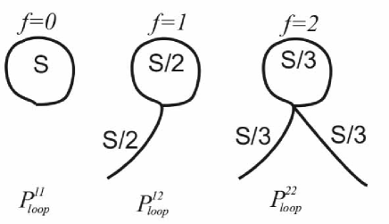
Figure 1: Schematic presentation of loops with different positions along the polymer chain.

In this concern, it is worthwhile to study a probability of loop formation in the environment with long range correlated disorder, which has not been considered so far. In the present paper, we analyze this problem analytically within the frames of continuous chain model, applying the direct polymer renormalization scheme. The layout of the paper is as follows. In the next Section, we introduce the model. The direct polymer renormalization scheme is shortly described in Section III. We present the results obtained for critical exponents in Section IV and end up with giving conclusions in Section V.

II The Model

We start with considering a flexible polymer chain in solution in presence of long-range correlated disorder. Within the Edwards continuous chain model Edwards , the chain is presented as a continuous path of length $S$, parametrized by $\vec{r}(s)$, where $s$ changes from $0$ to $S$. To describe the presence of loop with certain position along the chain (see Fig. 1), we consider the system of ring polymer connected with $f$ linear chains (with $f=0,1,2$), so that $f=0$ corresponds to a loop formed by two end monomers of the chains, $f=1$ – a loop formed by inner monomer and end one, $f=2$ – an inner loop. Thus, our problem can be considered as a particular case of so-called rosette polymer structures, studied recently in Ref. Metzler15 .

The partition function of the system can thus be presented as:

$${\cal Z}_{1;f}(S)=\frac{{\displaystyle{\int}}\!{\cal{D}}\vec{r}\,\,\delta(\vec{r}_{1}(S)-\vec{r}_{1}(0)){\displaystyle{\prod\limits_{i=1}^{1+f_{2}}}}\delta(\vec{r}_{i}(0)){\rm e}^{-H}}{{\displaystyle{\int}}\!{\cal{D}}\vec{r}\,\,{\displaystyle{\prod\limits_{i=1}^{1+f}}}\delta(\vec{r}_{i}(0)){\rm e}^{-H}}.$$ (10)

Here, $\int\!{\cal D}{\vec{r}}$ denotes functional path integrations over $1+f$ trajectories, the $\delta$-functions describe the fact that one trajectory is closed and that the starting point of all $1+f$ trajectories is fixed, and $H$ is a Hamiltonian of the system:

$$H=\sum_{i=1}^{1+f}\frac{1}{2}\int^{\frac{S}{1+f}}_{0}{\rm d}s\,\left(\frac{{\rm d}\vec{r}_{i}(s)}{ds}\right)^{2}+$$

$$+\frac{u_{0}}{2}\sum_{i,j=1}^{1+f}\int^{\frac{S}{1+f}}_{0}{\rm d}s^{\prime}\int^{s^{\prime}}_{0}{\rm d}s^{\prime\prime}\delta(\vec{r}_{i}(s^{\prime})-\vec{r}_{j}(s^{\prime\prime}))-$$

$$-\sum_{i=1}^{1+f}\int^{\frac{S}{1+f}}_{0}{\rm d}s\,V(\vec{r}_{i}(s)),$$ (11)

where the first term describes connectivity of trajectories, the second term describes short-range repulsion between monomers due to excluded volume effect governed by coupling constant $u_{0}$ and the last one arises due to the presence of disorder in the system and contains a random potential $V(\vec{r}(s))$. Let us denote by ${\overline{(\ldots)}}$ the average over different realizations of disorder and assume Weinrib83 :

$${\overline{V(\vec{r}_{i}(s^{\prime}))V(\vec{r}_{j}(s^{\prime\prime}))}}=w_{0}|\vec{r}_{i}(s^{\prime})-\vec{r}_{j}(s^{\prime\prime})|^{-a},$$ (12)

where $w_{0}$ is a corresponding coupling constant. Performing the averaging of the partition function (10) over different realizations of disorder, taking into account up to the second moment of cumulant expansion and recalling (12) we obtain ${\overline{{\cal Z}_{1;f}(S)}}$ with an effective Hamiltonian:

$$H_{eff}=\frac{1}{2}\sum_{i=1}^{1+f}\int_{0}^{\frac{S}{1+f}}{\rm d}s\!\left(\frac{{\rm d}{\vec{r}}_{i}(s)}{{\rm d}s}\right)^{2}+$$ (13)

$$+\frac{u_{0}}{2}\sum_{i,j=1}^{1+f}\int^{\frac{S}{1+f}}_{0}ds^{\prime}\int^{s^{\prime}}_{0}ds^{\prime\prime}\delta(\vec{r}_{i}(s^{\prime})-\vec{r}_{j}(s^{\prime\prime}))\,ds-$$

$$-\frac{w_{0}}{2}\sum_{i,j=1}^{1+f}\int_{0}^{\frac{S}{1+f}}{\rm d}s^{\prime}\int_{0}^{S}{\rm d}s{{}^{\prime\prime}}\,|\vec{r}_{i}(s^{\prime\prime})-\vec{r}_{j}(s^{\prime})|^{-a}.$$

The probabilities of loop formations (5) can be thus calculated as:

$$P_{{\rm loop}}^{11}=\frac{{\overline{{\cal Z}_{1;0}(S)}}}{{\overline{{\cal Z}(S)}}}\sim S^{\lambda_{11}},$$

$$P_{{\rm loop}}^{12}=\frac{{\overline{{\cal Z}_{1;1}(S)}}}{{\overline{{\cal Z}(S)}}}\sim\left(\frac{S}{2}\right)^{\lambda_{12}},$$

$$P_{{\rm loop}}^{22}=\frac{{\overline{{\cal Z}_{1;2}(S)}}}{{\overline{{\cal Z}(S)}}}\sim\left(\frac{S}{3}\right)^{\lambda_{22}},$$ (14)

where ${{\overline{{\cal Z}(S)}}}$ is the total partition function of linear chain of length $S$ given by:

$${\overline{{\cal Z}(S)}}=\displaystyle{\int}\!{\cal{D}}\vec{r}\,\exp\left[\frac{1}{2}\int_{0}^{S}{\rm d}s\!\left(\frac{{\rm d}{\vec{r}}(s)}{{\rm d}s}\right)^{2}+\right.$$

$$+\frac{u_{0}}{2}\int^{S}_{0}{\rm d}s^{\prime}\int^{s^{\prime}}_{0}{\rm d}s^{\prime\prime}\delta(\vec{r}(s^{\prime})-\vec{r}(s^{\prime\prime}))\,ds-$$

$$-\left.\frac{w_{0}}{2}\int_{0}^{S}{\rm d}s^{\prime}\int_{0}^{S}{\rm d}s{{}^{\prime\prime}}\,|\vec{r}(s^{\prime\prime})-\vec{r}(s^{\prime})|^{-a}\right].$$ (15)

III The Method

We apply the direct renormalization method developed by des Cloizeaux desCloiseaux . The main idea of this technique is to eliminate various divergences, observed in the asymptotic limit of an infinitely long polymer chain (corresponding to an infinite number of configurations) by introducing corresponding renormalization factors directly associated with physical quantities. In particular, the renormalization factor $\chi_{1}(\{z_{0}\})$ (with $\{z_{0}\}$ being the set of bare coupling constants) is introduced via:

$$\frac{{\cal Z}(S)}{{\cal Z}^{{\rm Gauss}}(S)}=\chi_{1}(\{z_{0}\}).$$ (16)

Here, ${\cal Z}(S)$ is the partition function of single polymer chain and ${\cal Z}^{{\rm Gauss}}(S)$ is the partition function of an idealized Gaussian model. It is established that the number of all possible conformations of polymer chain scales with the weight of a macromolecule parametrised by $S$ as:

$${\cal Z}(S)\sim\mu^{S}S^{\gamma-1},$$ (17)

where $\gamma$ is the universal critical exponent depending only on the space dimension $d$ and $\mu$ is a non-universal fugacity. From the scaling assumption (17) one finds an estimate for an effective critical exponent $\gamma(\{z_{0}\})$ governing the scaling behavior of the number of possible configurations as:

$$\gamma(\{z_{0}\})-1=S\frac{\partial\ln\chi_{1}(\{z_{0}\})}{\partial S}.$$ (18)

In a similar way, in our problem we may introduce the factors $\chi_{ab}(\{z_{0}\})$ via:

$$\frac{P_{{\rm loop}}^{ab}}{P_{{\rm loop}}^{{\rm Gauss}}}=\chi_{ab}(\{z_{0}\})$$ (19)

with $a,b=1,2$. Recalling the scaling of loop probabilities (14) and remembering the fact that in Gaussian approximation $P_{{\rm loop}}^{{\rm Gauss}}\sim S^{-d/2}$, one finds an estimate for the effective critical exponents $\lambda_{ab}(\{z_{0}\})$:

$$\lambda_{ab}(\{z_{0}\})-d/2=-S\frac{\partial\ln\chi_{ab}(\{z_{0}\})}{\partial S}\,.$$ (20)

The critical exponents presented in the form of series expansions in the coupling constants are divergent in the asymptotic limit of large $S$. To eliminate these divergences, the renormalization of the coupling constants is performed. The critical exponents attain finite values when evaluated at a stable fixed point of the renormalization group transformation. The flows of the renormalized coupling constants are governed by functions $\beta_{z_{\mathrm{R}}}$:

$$\beta_{z_{\mathrm{R}}}=2S\frac{\partial z_{\mathrm{R}}(\{z_{0}\})}{\partial S}\,.$$ (21)

Reexpressing $\{z_{0}\}$ in terms of renormalized couplings $z_{\mathrm{R}}$, the fixed points of renormalization group transformations are given by common zeros of the $\beta$-functions. Stable fixed points govern the asymptotical scaling properties of macromolecules and gives reliable asymptotical values of the critical exponents (20) .

IV Results

We start with evaluating the partition function ${\cal Z}_{1;f}(S)$ in the simplified Gauusian case, which is then given by:

$${\cal Z}_{1;f}(S)=\frac{{\displaystyle{\int}}\!{\cal{D}}\vec{r}\,\,\delta(\vec{r}_{1}(S)-\vec{r}_{1}(0)){\displaystyle{\prod\limits_{i=1}^{1+f_{2}}}}\delta(\vec{r}_{i}(0)){\rm e}^{-H_{0}}}{{\displaystyle{\int}}\!{\cal{D}}\vec{r}\,\,{\displaystyle{\prod\limits_{i=1}^{1+f}}}\delta(\vec{r}_{i}(0)){\rm e}^{-H_{0}}}.$$ (22)

where $H_{0}=\frac{1}{2}\sum\limits_{i=1}^{1+f}\int\limits_{0}^{S/(1+f)}{\rm d}s\,\left(\frac{{\rm d}{\vec{r}}_{i}(s)}{{\rm d}s}\right)^{2}$. Using the Fourier-transform of the $\delta$-functions

$$\delta(\vec{r}_{1}(S)-\vec{r}_{1}(0))=(2\pi)^{-d}\int{\rm d}\vec{q}_{1}\,{\rm e}^{-i\vec{q}_{1}(\vec{r}_{1}(S)-\vec{r}_{1}(0))}\,,$$ (23)

we receive

$${\cal Z}_{1;f}(S)=(2\pi)^{-d}\int{\rm d}\vec{q}_{1}\,{\rm e}^{-\frac{q_{1}^{2}S}{2}}=(2\pi S)^{-d/2}.$$ (24)

In Gaussian approximation the value of partition function does not depend on $f$, and thus the looping probability is independent on the loop position along the chain according to Ref. Jacobson50 .

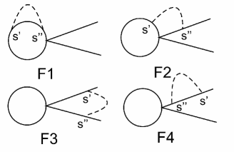
Figure 2: Diagrammatic presentation of contributions into the partition function $Z_{1;2}$ up to the first order in the coupling constants.

Taking into account the excluded volume effect and presence of disorder, we present the partition function as perturbation theory series in dimensionless coupling constants $z_{u}{=}u_{0}(2\pi)^{-d/2}S^{2-d/2}$ and $z_{w}{=}w_{0}(2\pi)^{-a/2}S^{2-a/2}$:

$${\cal Z}_{1;f}(S)=(2\pi S)^{-d/2}-z_{u}Z^{u}_{1;f}+z_{w}Z^{w}_{1;f}+\ldots$$ (25)

It is convenient to present the contributions into $Z^{u}_{1;f}$ and $Z^{w}_{1;f}$ using the diagrammatic technique (Fig. 2). Here, dotted lines denote possible interactions between points $s^{\prime}$ and $s^{\prime\prime}$ governed by couplings $z_{u}$ and $z_{w}$, and integrations are to be performed over all positions of the segment end points. Note that contributions into $Z_{1;0}$ are given by only the first diagram and correspond to the partition function of the ring polymer Haydukivska14 . On the other hand, contributions into partition function $Z_{1;1}$ are given by all diagrams except $F_{3}$. The analytical expressions corresponding to contributions of diagrams $F_{1}$-$F_{4}$ into $Z^{u}_{1;f}$ read:

$${F_{1}}^{u}_{f}=z_{u}\int_{0}^{S/(1+f)}{\rm d}s^{\prime}\int^{s^{\prime}}_{0}{\rm d}s^{\prime\prime}(2\pi)^{-2d}\times$$

$$\times\int{\rm d}\vec{q}\,{\rm d}\vec{r}\,\exp\left(-\frac{\vec{q}^{2}}{2}S_{f}-\frac{\vec{p}^{2}}{2}(s^{\prime}-s^{\prime\prime})-\vec{q}\vec{p}(s^{\prime}-s^{\prime\prime})\right),$$

$${F_{2}}^{u}_{f}=z_{u}\int_{0}^{S/(1+f)}\,{\rm d}s^{\prime}\int^{S_{f}}_{0}\,{\rm d}s^{\prime\prime}(2\pi)^{-2d}\times$$

$$\times\int\,{\rm d}\vec{q}\,{\rm d}\vec{r}\,\exp\left(-\frac{\vec{q}^{2}}{2}S_{f}-\frac{\vec{p}^{2}}{2}(S_{f}-s^{\prime\prime}+s^{\prime})-\vec{q}\vec{p}s^{\prime}\right),$$

$${F_{3}}^{u}_{f}=z_{u}\int_{0}^{S/(1+f)}\,{\rm d}s^{\prime}\int^{S_{f}}_{0}\,{\rm d}s^{\prime\prime}(2\pi)^{-2d}\times$$

$$\times\int\,{\rm d}\vec{q}\,{\rm d}\vec{r}\,\exp\left(-\frac{\vec{q}^{2}}{2}S_{f}-\frac{\vec{p}^{2}}{2}(s^{\prime}+s^{\prime\prime})\right),$$

$${F_{4}}^{u}_{f}=z_{u}\int_{0}^{S/(1+f)}\,{\rm d}s^{\prime}\int^{s^{\prime}}_{0}\,{\rm d}s^{\prime\prime}(2\pi)^{-2d}\times$$

$$\times\int\,{\rm d}\vec{q}\,{\rm d}\vec{r}\,\exp\left(-\frac{\vec{q}^{2}}{2}S_{f}-\frac{\vec{p}^{2}}{2}(s^{\prime}-s^{\prime\prime})\right).$$

Performing the integrations, we get:

$${F_{1}}^{u}_{f}=z_{u}\left(2\pi\frac{S}{1+f}\right)^{-d/2}B\left(1-\frac{d}{2},2-\frac{d}{2}\right),$$

$${F_{2}}^{u}_{f}=z_{u}\left(2\pi\frac{S}{1+f}\right)^{-d/2}\left[\left(1-\frac{d}{2}\right)^{-1}\times\right.$$

$$\left.\times\left(\frac{5}{4}\right)^{1-d/2}H(1/2;-1+d/2,3/2;1/5)-\right.$$

$$\left.-\left(1-\frac{d}{2}\right)^{-1}B\left(2-\frac{d}{2},2-\frac{d}{2}\right)\right],$$

$${F_{3}}^{u}_{f}=z_{u}\left(2\pi\frac{S}{1+f}\right)^{-d/2}(2^{2-d/2}-2)\times$$

$$\times\left(1-\frac{d}{2}\right)^{-1}\left(2-\frac{d}{2}\right)^{-1},$$

$${F_{4}}^{u}_{f}=z_{u}\left(2\pi\frac{S}{1+f}\right)^{-d/2}\left(1-\frac{d}{2}\right)^{-1}\left(2-\frac{d}{2}\right)^{-1},$$

here, $B$ is Euler Beta-function and $H$ is hypergeometric function.

As a result, we obtain contributions into the partition function in the form:

$$Z^{u}_{1;0}=z_{u}(2\pi S)^{-d/2}B\left(1-\frac{d}{2},2-\frac{d}{2}\right),$$

$$Z^{u}_{1;1}=z_{u}\left(2\pi\frac{S}{2}\right)^{-d/2}\left[B\left(1-\frac{d}{2},2-\frac{d}{2}\right)+\right.$$

$$\left.+\left(1-\frac{d}{2}\right)^{-1}\left(2-\frac{d}{2}\right)^{-1}-\right.$$

$$\left.-\left(1-\frac{d}{2}\right)^{-1}B\left(2-\frac{d}{2},2-\frac{d}{2}\right)+\right.$$

$$\left.+\left(1-\frac{d}{2}\right)^{-1}\left(\frac{5}{4}\right)^{1-d/2}H(1/2;-1+d/2,3/2;1/5)\right],$$

$$Z^{u}_{1;2}=z_{u}\left(2\pi\frac{S}{3}\right)^{-d/2}\left[B\left(1-\frac{d}{2},2-\frac{d}{2}\right)+\right.$$

$$\left.+(2^{2-d/2})\left(1-\frac{d}{2}\right)^{-1}\left(2-\frac{d}{2}\right)^{-1}-\right.$$

$$\left.-2\left(1-\frac{d}{2}\right)^{-1}B\left(2-\frac{d}{2},2-\frac{d}{2}\right)+\right.$$

$$\left.+2\left(1-\frac{d}{2}\right)^{-1}\left(\frac{5}{4}\right)^{1-d/2}H(1/2;-1+d/2,3/2;1/5)\right].$$

Note, that corresponding contributions into $Z^{w}_{1;f}$ are obtained simply by substituting $z_{u}$ by $z_{w}$ and $d$ by $a$ in expressions in square brackets in above relations.

Performing a double expansion over parameters $\varepsilon=4-d$, $\delta=4-a$ we finally receive the expressions for partition functions for the chains with a loop of certain type:

$$\overline{{\cal Z}_{1,0}}(S)=(2\pi S)^{-d/2}\left(1-z_{u}\left(\frac{4}{\varepsilon}-2\right)+\right.$$

$$\left.+z_{w}\left(\frac{4}{\delta}-2\right)\right),$$

$$\overline{{\cal Z}_{1,1}}(S)=\left(2\pi\frac{S}{2}\right)^{-d/2}\left(1-z_{u}\left(\frac{6}{\varepsilon}-1+\right.\right.$$

$$\left.+\frac{2}{\sqrt{5}}(\ln 2-\ln(3+\sqrt{5}))\right)+$$

$$\left.+z_{w}\left(\frac{6}{\delta}-1+\frac{2}{\sqrt{5}}(\ln 2-\ln(3+\sqrt{5}))\right)\right),$$

$$\overline{{\cal Z}_{1,2}}(S)=\left(2\pi\frac{S}{3}\right)^{-d/2}\left(1-z_{u}\left(\frac{10}{\varepsilon}+1-\right.\right.$$

$$\left.-\ln 2+\frac{2}{\sqrt{5}}(\ln 2-\ln(3+\sqrt{5}))\right)+z_{w}\left(\frac{10}{\delta}+\right.$$

$$\left.\left.+1-\ln 2+\frac{2}{\sqrt{5}}(\ln 2-\ln(3+\sqrt{5}))\right)\right).$$ (26)

In addition, the total partition function of linear chain of length $S$ is given by:

$$\overline{{\cal Z}}(S)=1-z_{u}\left(-\frac{2}{\varepsilon}-1\right)+z_{w}\left(-\frac{2}{\delta}-1\right).$$ (27)

Probabilities of loops formations are received using the definition (14) and read:

$$P^{11}_{{\rm loop}}=(2\pi S)^{-d/2}\left(1-z_{u}\left(\frac{6}{\varepsilon}-1\right)+\right.$$

$$\left.+z_{w}\left(\frac{6}{\delta}-1\right)\right),$$

$$P^{12}_{{\rm loop}}=\left(2\pi\frac{S}{2}\right)^{-d/2}\left(1-z_{u}\left(\frac{8}{\varepsilon}+\frac{2}{\sqrt{5}}(\ln 2-\right.\right.$$

$$\left.\left.-\ln(3+\sqrt{5}))\right)+z_{w}\left(\frac{8}{\delta}+\frac{2}{\sqrt{5}}(\ln 2-\right.\right.$$

$$\left.\left.-\ln(3+\sqrt{5}))\right)\right),$$

$$P^{22}_{{\rm loop}}=\left(2\pi\frac{S}{3}\right)^{-d/2}\left(1-z_{u}\left(\frac{12}{\varepsilon}+2-\right.\right.$$

$$\left.-\ln 2+\frac{2}{\sqrt{5}}(\ln 2-\ln(3+\sqrt{5}))\right)+$$

$$\left.+z_{w}\left(\frac{12}{\delta}+2-\ln 2+\right.\right.$$

$$\left.\left.+\frac{2}{\sqrt{5}}(\ln 2-\ln(3+\sqrt{5}))\right)\right).$$ (28)

Recalling that (20) can be presented in the form

$$\lambda_{ab}-d/2=-\frac{\varepsilon}{2}\frac{1}{\chi_{ab}}\frac{\partial\chi_{ab}}{\partial z_{u}}z_{u}-\frac{\delta}{2}\frac{1}{\chi_{ab}}\frac{\partial\chi_{ab}}{\partial z_{w}}z_{w}$$ (29)

we find for the critical exponents governing the scaling of looping probabilities:

$$\lambda_{11}=(4-\varepsilon/2)+\frac{\varepsilon}{2}\left(\frac{6}{\varepsilon}-1\right)z_{u}-\frac{\delta}{2}\left(\frac{6}{\delta}-1\right)z_{w}$$

$$\lambda_{12}=(4-\varepsilon/2)+\frac{\varepsilon}{2}\left(\frac{8}{\varepsilon}+\frac{2}{\sqrt{5}}(\ln 2-\right.$$

$$\left.-\ln(3+\sqrt{5}))\right)z_{u}-$$

$$-\frac{\delta}{2}\left(\frac{8}{\delta}+\frac{2}{\sqrt{5}}(\ln 2-\ln(3+\sqrt{5}))\right)z_{w},$$

$$\lambda_{22}=(4-\varepsilon/2)+\frac{\varepsilon}{2}\left(\frac{12}{\varepsilon}+2-\ln 2+\right.$$

$$\left.+\frac{2}{\sqrt{5}}(\ln 2-\ln(3+\sqrt{5}))\right)z_{u}-$$

$$-\frac{\delta}{2}\left(\frac{12}{\delta}+2-\ln 2+\right.$$

$$+\left.\frac{2}{\sqrt{5}}(\ln 2-\ln(3+\sqrt{5}))\right)z_{w}.$$ (30)

Taking into account that $z_{u}$ and $z_{w}$ in the first order of perturbation theory are proportional to $\varepsilon$, $\delta$, and keeping only contributions up to $\varepsilon$ and $\delta$, the above expressions can be presented as:

$$\lambda_{11}=2-\varepsilon/2+3z_{u}-3z_{w},$$ (31)

$$\lambda_{12}=2-\varepsilon/2+4z_{u}-4z_{w},$$ (32)

$$\lambda_{22}=2-\varepsilon/2+6z_{u}-6z_{w}.$$ (33)

Figure 3: Scaling exponents (37) and (38) as function of $\delta=4-a$ in $d=3$.

We make use of results for fixed point values found previously for the linear polymer chains in long-range correlated disorder Blavatska01 . There are three distinct fixed points governing the properties of macromolecule in various regions of parameters $d$ and $a$:

$${\rm{Gaussian}}:z^{*}_{u_{0}}=0,z^{*}_{w_{0}}=0,$$ (34)

$${\rm{Pure}}:z^{*}_{u_{0}}=\frac{\varepsilon}{8},z^{*}_{w_{0}}=0,$$ (35)

$${\rm{mixedLR}}:z^{*}_{u_{0}}=\frac{\delta^{2}}{4(\varepsilon-\delta)},z^{*}_{w_{0}}=\frac{\delta(\varepsilon-2\delta)}{4(\delta-\varepsilon)}.$$ (36)

Evaluating Eqs. (31) - (33) at Gaussian fixed point, we restore the result of Jacobson and Stockmayer Jacobson50 : $\lambda^{{\rm Gauss}}=d/2$. For polymers with excluded volume effect in pure solutions we restore results of Duplantier Duplantier89 :

$$\lambda^{{\rm pure}}_{0}=2-\varepsilon/8,$$

$$\lambda^{{\rm pure}}_{1}=2,$$

$$\lambda^{{\rm pure}}_{2}=2+\varepsilon/4.$$ (37)

Finally, for the considered case of a polymer chain in disordered environment we received a brand new results:

$$\lambda^{{\rm LR}}_{0}=2-\varepsilon/2+3\delta/4,$$

$$\lambda^{{\rm LR}}_{1}=2-\varepsilon/2+\delta,$$

$$\lambda^{{\rm LR}}_{2}=2-\varepsilon/2+3\delta/2.$$ (38)

To find the quantitative estimate for the exponents (37) and (38) at $d{=}3$, we evaluate the expressions at $\varepsilon{=}1$ and various fixed values of $\delta$ (see Fig. 3). We find, that presence of long-range correlated disorder with any $a{<}d$ leads to an increase of exponents as compared with corresponding pure values, and thus the probabilities of loop formation decreases in presence of crowded environment. From physical point of view, we can interpret this as follows. The presence of complex (fractal) obstacles in the system forces the macromolecule to avoid these extended regions of space, which results in effective elongation of polymer chain and makes the contact of two monomers along the chain less probable.

V Conclusions

In present work we analyzed a probability of loop formation in flexible polymer chains in good solutions, which is known to be governed by scaling laws (5) with scaling exponents $\lambda$ dependent on the position of loop along the macromolecule. We considered the special case, when structural obstacles are present in the environment, which are assumed to be correlated on large distances $r$ according to a power law with a pair correlation function $g(r)\sim r^{-a}$ with $a<d$ Weinrib83 . The previous studies Blavatska01 ; Blavatska10 ; Haydukivska14 reveal the non-trivial impact of such a type of disorder on the universal conformational properties of both linear and closed ring macromolecules.

Working within the frames of continuous chain model and applying the direct polymer renormalization scheme, we obtain the values of critical exponents $\lambda$ up to the first order of perturbation theory in parameters $\varepsilon=4-d$, $\delta=4-a$. Our results quantitatively reveal that presence of long-range correlated disorder with any $a<d$ leads to an increase of exponents as compared with corresponding pure values, and thus the probabilities of loop formation decreases in presence of crowded environment.

References

(1)
L.J. Perry and R. Wetzel, Science 226, 555 (1984).
(2)
J.A. Wells and D.B. Powers, J. Biol. Chem. 261, 6564 (1986).
(3)
C.N. Pace, G.R. Grimsley, J.A. Thomson, and B.J. Barnett, J. Biol. Chem. 263, 11820 (1988).
(4)
A.D. Nagi and L. Regan, Folding Des. 2, 67 (1997).
(5)
R. Schlief, Science 240, 127 (1988).
(6)
K. Rippe, P.H. von Hippel, and J. Langowski, Trends. Biochem. Sci. 20, 500 (1995).
(7)
K. B. Towles, J.F. Beausang, H.G. Garcia, R. Phillips, and P.C. Nelson, Phys. Biol. 6, 025001 (2009).
(8)
P. Fraser, Curr. Opin. Genet. Dev. 16, 490 (2006).
(9)
M. Simonis, P. Klous, E. Splinter, Y. Moshkin, R. Willemsen, E. de Wit, B. van Steensel, and W. de Laat, Nat. Genet. 38, 1348 (2006).
(10)
J. Dorier and A. Stasiak, Nucl. Acids Res. 37, 6316 (2009).
(11) P.G. de Gennes, Scaling Concepts in Polymer Physics (Cornell
University Press, Ithaca, 1979).
(12) J. des Cloizeaux and G. Jannink, Polymers in Solutions: Their
Modelling and Structure (Clarendon Press, Oxford, 1990).
(13)
B. Nienhuis, Phys. Rev. Lett. 49, 1062 (1982).
(14)
R. Guida and J. Zinn-Justin, J. Phys. A 31, 8104 (1998).
(15) H. Jacobsond and W.H. Stockmayer, J. Chem. Phys. 18, 1600 (1950).
(16) H.S. Chan and K.A. Dill, J. Chem. Phys. 90, 492(1989).
(17) S. Redner, J. Phys. A 13, 3525 (1980).
(18) B. Duplantier, J. Stat. Phys. 54, 581 (1989).
(19) H.P. Hsu, W. Nadler, and P. Grassberger, Macromol;ecules 37, 4658 (2004).
(20)
A.M. Rubio, J.J. Freire, M. Bishop, and
J.H.R. Clarke, Macromolecules 26, 4018 (1993).
(21)
P.N. Pusey and W. van Megen, Nature 320, 340 (1986).
(22)
S. Kumar and M.S. Li, Phys. Rep. 486, 1 (2010).
(23)
A. Minton, J. Biol. Chem. 276, 10577 (2001).
(24)
Y. Kim, J. Phys. C 16, 1345 (1983).
(25)
K. Kremer, Z. Phys. B: Condens. Matter 49, 149 (1981).
(26)
S.B. Lee and H. Nakanishi, Phys. Rev. Lett. 61,2022 (1988).
(27)
K.Y. Woo and S.B. Lee,
Phys. Rev. A 44, 999 (1991).
(28)
P. Grassberger, J. Phys. A: Math. Gen. 26, 1023 (1993).
(29)
A. Ordemann, M. Porto, H.E. Roman, S. Havlin, and A. Bunde, Phys. Rev. E 61, 6858 (2000).
(30)
H.-K. Janssen and O. Stenull, Phys. Rev. E 75, 020801R (2007).
(31)
A.L. Dullen, Porous Media: Fluid Transport and Pore Structure (Academic, New York, 1979).
(32)A. Weinrib and B.I. Halperin,
Phys. Rev. B 27, 413 (1983).
(33)
V. Blavats’ka, C. von Ferber, and Yu. Holovatch, J. Mol. Liq. 91
77 (2001); Phys. Rev. E 64 041102 (2001).
(34)
V. Blavatska, C. von Ferber, and Yu. Holovatch, Phys. Lett. A 374, 2861 (2010).
(35)
K. Haydukivska and V. Blavatska, J. Chem. Phys. 141, 094906 (2014).
(36)
S.F. Edwards, Proc. Phys. Soc. Lond. 85, 613 (1965);
Proc. Phys. Soc. Lond. 88, 265 (1965).
(37)
V. Blavatska and R. Metzler, J. Phys. A: Math. Theor. 48, 135001 (2015).