Wireless Powered Cooperative Jamming for Secrecy Multi-AF Relaying Networks

Abstract

This paper studies secrecy transmission with the aid of a group of wireless energy harvesting (WEH)-enabled amplify-and-forward (AF) relays performing cooperative jamming (CJ) and relaying. The source node in the network does simultaneous wireless information and power transfer (SWIPT) with each relay employing a power splitting (PS) receiver in the first phase; each relay further divides its harvested power for forwarding the received signal and generating artificial noise (AN) for jamming the eavesdroppers in the second transmission phase. In the centralized case with global channel state information (CSI), we provide closed-form expressions for the optimal and/or suboptimal AF-relay beamforming vectors to maximize the achievable secrecy rate subject to individual power constraints of the relays, using the technique of semidefinite relaxation (SDR), which is proved to be tight. A fully distributed algorithm utilizing only local CSI at each relay is also proposed as a performance benchmark. Simulation results validate the effectiveness of the proposed multi-AF relaying with CJ over other suboptimal designs.

I Introduction

Wireless powered communication network has arisen as a new system with stable and self-sustainable power supplies in shaping future-generation wireless communications [1, 2]. The enabling technology, known as simultaneous wireless information and power transfer (SWIPT), has particularly drawn an upsurge of interests owing to the far-field electromagnetic power carried by radio-frequency (RF) signals that affluently exist in wireless communications. With the transmit power, waveforms, and dimensions of resources, etc., being all fully controllable, SWIPT promises to prolong the lifetime of wireless devices while delivering the essential communication functionality, as will be important for low-power applications such as RF identification (RFID) and wireless sensor networks (WSNs) (see [3, 4] and the references therein).

On the other hand, privacy and authentication have increasingly become major concerns for wireless communications and physical (PHY)-layer security has emerged as a new layer of defence to realize perfect secrecy transmission in addition to the costly upper-layer techniques such as cryptography. In this regard, relay-assisted secure transmission was proposed [6, 5] and PHY-layer security enhancements by means of cooperative communications have since attracted much attention [7, 8, 9, 10, 11, 12, 13, 15, 16, 17, 18, 19, 20, 14].

In particular, cooperative schemes can be mainly classified into three categories: decode-and-forward (DF), amplify-and-forward (AF), and cooperative jamming (CJ) [7] with CJ being most relevant to PHY-layer security. Specifically, coordinated CJ refers to the scheme of generating a common jamming signal across all single-antenna relay helpers against eavesdropping [7, 12, 13, 10], while uncoordinated CJ considers that each relay helper emits independent artificial noise (AN) to confound the eavesdroppers [15, 16]. It is expected that in the scenarios where the direct link is broken between the transmitter (Tx) and the legitimate receiver (Rx), some of the relays have to take on their conventional role of forwarding the information while others will perform CJ [17, 18]. A recent paradigm that generalizes all the above-mentioned cooperation strategies is cooperative beamforming (CB) mixed with CJ [19, 20], where the available power at each relay is split into two parts: one for forwarding the confidential message and the other for CJ.

However, mixed CB-CJ approaches may be prohibitive in applications with low power devices because idle relays with limited battery supplies would likely prefer saving power for their own traffic to assisting others’ communication. In light of this, SWIPT provides the incentive for potential helpers to perform dedicated CB mixed with CJ at no expense of its own power, but opportunistically earn harvested energy. Motivated by this, our work considers secrecy transmission from a Tx to a legitimate Rx with the aid of a set of single-antenna wireless energy harvesting (WEH)-enabled AF-operated relays in the presence of multiple single-antenna eavesdroppers. As a matter of fact, cooperative schemes that involve WEH-enabled relays was recently investigated in [21]. We consider the use of the dynamic power splitting (DPS) receiver architecture, initially proposed for SWIPT in [22], which divides the received power with an adjustable ratio for energy harvesting (EH) and information receiving (IR). WEH-enabled relays using DPS receivers have also been considered in [23, 24, 25] and [26, 27, 29], without (w/o) and with secrecy consideration, respectively. Note that there is also interest in addressing the threat that WEH receivers may attempt to intercept the confidential messages in SWIPT-enabled networks [29, 28, 30, 31]. Nevertheless, we will focus on exploiting the benefits of WEH-enabled relays when they are trustful.

In particular, motivated by the strong interest in SWIPT and the vast degree-of-freedom (DoF) achievable by cooperative relays, this paper aims to maximize the secrecy rate with the aid of WEH-enabled AF-operated relays, subject to the EH power constraints of individual relays by jointly optimizing the CB of the relays and the CJ covariance matrix. In this paper, we assume that there is no direct link between the source and destination nodes, and perfect global channel state information (CSI) is available for the case of centralized optimization.

It is worth pointing out that although our setting may look similar to [20], their optimal CB-CJ design is not applicable to ours due to the multiplicative nature in beamforming weights incurred by the power splitting (PS) ratios that intrinsically poses more intractability to our optimization problem. Further, our work also differs from [27] where an efficient algorithm was proposed to maximize the secrecy rate for the optimization of the PS ratios and AF relay beamforming. The difference is twofold. First, AN was not considered in the second transmission phase in [27] and in addition, their algorithm only converged to a local optimum, as opposed to our work that gives the global optimal solutions for CB.

The rest of the paper is organized as follows. Section II describes two types of WEH-enabled Rx architecture for the AF relays and defines the secrecy rate region of the relay wiretap channel. Section III then formulates the secrecy rate maximization problems that jointly optimize the AN (or CJ) and the AF-relay CB for the WEH-enabled relays operating with the two types of Rx. The problems are respectively solved by centralized schemes in Section IV and distributed approaches in Section V. Section VI provides simulation results to evaluate the performance of the proposed schemes. Finally, Section VII concludes the paper.

Notations—We use the uppercase boldface letters for matrices and lowercase boldface letters for vectors. The superscripts $(\cdot)^{T}$, $(\cdot)^{{\dagger}}$, $(\cdot)^{H}$ and $(\cdot)^{\ast}$ represent, respectively, the transpose, conjugate, conjugate transpose operations on vectors or matrices, and the optimum. In addition, ${\rm trace}(\cdot)$ stands for the trace of a square matrix. Moreover, $[\cdot]_{i,j}$ denotes the $(i,j)$th entry of a matrix, while $\|\cdot\|$ and $\|\cdot\|.^{2}$ represent the Euclidean norm and the entry-wise absolute value square of a vector, respectively. Also, ${\rm diag}(\cdot)$ denotes a diagonal matrix with its diagonal specified by the given vector and $[\cdot]_{i=1}^{N}$ represents an $N\times 1$ vector with each element indexed by $i$. Furthermore, $\cdot$ and $\circ$ stand for product and Hadamard product, respectively. $\mathbb{C(R)}^{x\times y}$ denotes the field of complex (real) matrices with dimension $x\times y$ and ${\sf E[\cdot]}$ indicates the expectation operation. Finally, $(x)^{+}$ is short for $\max(0,x)$.

II System Model

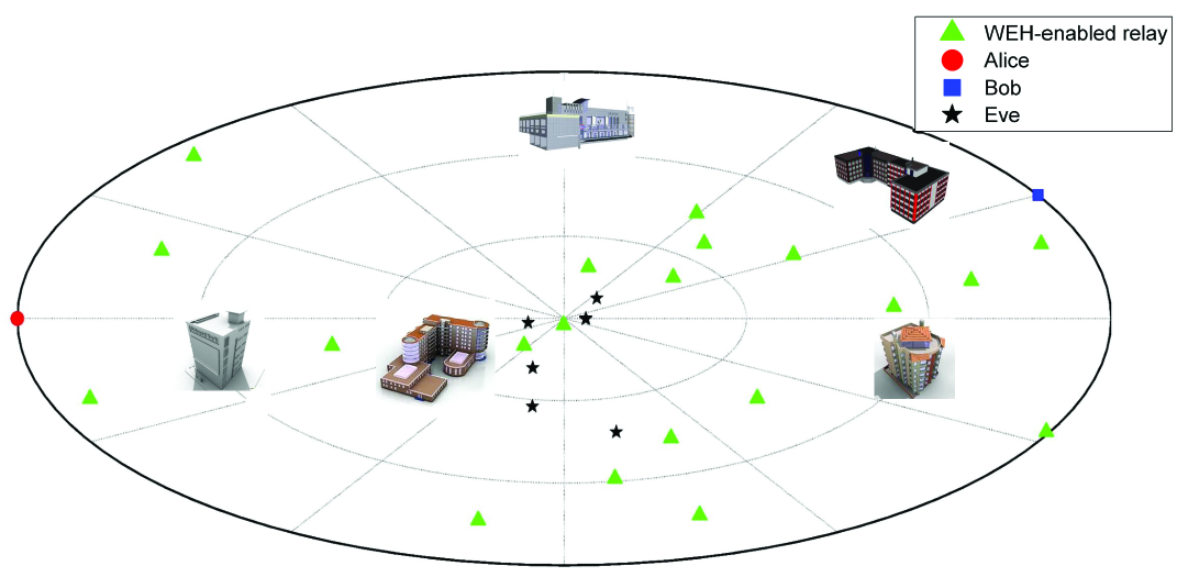
Figure 1: The system model for an AF relay-assisted SWIPT WSN.

In this paper, we consider secrecy transmission in a SWIPT-enabled WSN, where a Tx (Alice) wants to establish confidential communication with the legitimate Rx (Bob) with no direct link but with the aid of $N$ WEH-enabled sensors operating as AF relays, denoted by $\mathcal{N}=\{1,2,\ldots,N\}$, in the presence of multiple eavesdroppers (Eves), denoted by $\mathcal{K}=\{1,2,\ldots,K\}$, all equipped with single antenna. We assume that there is no direct link from the Tx to any of the Eves, due to, for instance, severe path loss or shadowing, as illustrated in Fig. 1.

We consider a two-hop relaying protocol based on two equal time slots and the duration of one transmit-slot is normalized to be one unit so that the terms “energy” and “power” are interchangeable with respect to (w.r.t.) one transmit-slot.

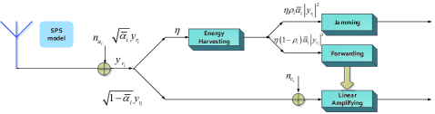
(a) WEH-enabled relay with SPS.

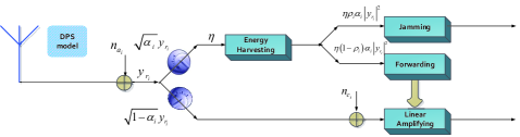
(b) WEH-enabled relay with DPS.

Figure 2: Architectures of the receiver for WEH-enabled relay.

At the receiver of each AF relay, we introduce two types of WEH-enabled receiver architecture, namely, static power splitting (SPS) (Fig. 2(a)) and DPS (Fig. 2(b)), both of which allow the relay to harvest energy and receive information from the same received signal. Specifically, the receiver first splits a portion of $\alpha_{i}$, of the received power for EH and the rest $1-\alpha_{i}$ for IR, $\forall i$. The $\alpha_{i}$ portion of harvested power is further divided into two streams with $\eta\rho_{i}\alpha_{i}|y_{r_{i}}|^{2}$ used for generating the AN to confound Eves and $\eta(1-\rho_{i})\alpha_{i}|y_{r_{i}}|^{2}$ used for amplifying the received signal, where $y_{r_{i}}$ is the $i$th element of the received signal $\boldsymbol{y}_{r}\in\mathbb{C}^{N\times 1}$, and $0\leq\eta<1$ denotes the EH efficiency. Note that DPS with adjustable $\alpha_{i}$’s is presently the most general receiver operation because practical circuits cannot directly decode the information from the stream used for EH [22] and SPS is just a special case of DPS with $\alpha_{i}=\bar{\alpha}_{i}$, $\forall i$, fixed for the whole transmission duration. However, SPS, advocated for its ease of implementation, is introduced separately in the sequel for its simplified relay beamforming design.

In the first transmit-slot, the received signal at each individual relay can be expressed as

$$y_{r_{i}}=h_{sr_{i}}\sqrt{P_{s}}s+n_{a,i},\;\forall i,$$ (1)

where the transmit signal $s$ is a circularly symmetric complex Gaussian (CSCG) random variable with zero mean and unit variance, denoted by $s\sim\mathcal{CN}(0,1)$, $h_{sr_{i}}$ denotes the complex channel from the Tx to the $i$th relay, $P_{s}$ is the transmit power at the Tx, and $n_{a,i}$ is the additive white Gaussian noise (AWGN) introduced by the receiving antenna of the $i$th relay, denoted by $n_{a,i}\sim\mathcal{CN}(0,\sigma_{n_{a}}^{2})$. As such, the linearly amplified baseband equivalent signal at the output of the $i$th relay is given by

$$x_{r_{i}1}=\beta_{i}(\sqrt{1-\alpha_{i}}y_{r_{i}}+n_{c,i}),\;\forall i,$$ (2)

where $\beta_{i}$ denotes the complex AF coefficient, and $n_{c,i}$ denotes the noise due to signal conversion from the RF band to baseband, denoted by $n_{c,i}\sim\mathcal{CN}(0,\sigma_{n_{c}}^{2})$. Since $x_{r_{i}1}$ is constrained by the portion of the harvested power for forwarding, i.e., $\eta(1-\rho_{i})\alpha_{i}|y_{r_{i}}|^{2}$, $\beta_{i}$ is accordingly given by

$$\beta_{i}=\sqrt{\frac{\eta(1-\rho_{i})\alpha_{i}|h_{sr_{i}}|^{2}P_{s}}{(1-\alpha_{i})|h_{sr_{i}}|^{2}P_{s}+(1-\alpha_{i})\sigma_{n_{a}}^{2}+\sigma_{n_{c}}^{2}}}e^{j\measuredangle\beta_{i}},$$ (3)

where $\measuredangle\beta_{i}$ denotes the phase of the AF coefficient for the $i$th relay.

Next, we introduce the CJ scheme. Denote the CJ signal generated from $N$ relays by $\boldsymbol{x}_{r2}=[x_{r_{1}2},\ldots,x_{r_{N}2}]^{T}$ and define its covariance matrix as $\boldsymbol{S}={\sf E}[\boldsymbol{x}_{r2}\boldsymbol{x}_{r2}^{H}]$. Then the coordinated CJ transmission can be uniquely determined by the truncated eigenvalue decomposition (EVD) of $\boldsymbol{S}$ given by $\boldsymbol{S}=\tilde{\boldsymbol{V}}\tilde{\boldsymbol{\Sigma}}\tilde{\boldsymbol{V}}^{H}$, where $\boldsymbol{\Sigma}={\rm diag}([\sigma_{1},\ldots,\sigma_{d}])$ is a diagonal matrix with $\sigma_{j}$’s denoting all the positive eigenvalues of $\boldsymbol{S}$ and $\boldsymbol{V}\in\mathbb{C}^{N\times d}$ is the precoding matrix satisfying $\boldsymbol{V}^{H}\boldsymbol{V}=\boldsymbol{I}$. Note that $d\leq N$ denotes the rank of $S$ which will be designed later. As a result, the CJ signal can be expressed as

$$\boldsymbol{x}_{r2}=\sum_{j=1}^{d}\sqrt{\sigma_{j}}\boldsymbol{v}_{j}s_{j}^{\prime},$$ (4)

where $\boldsymbol{v}_{j}$’s are drawn from the columns of $\boldsymbol{V}$, and $s_{j}^{\prime}$’s are independent and identically distributed (i.i.d.) complex Gaussian variables denoted by $s_{j}^{\prime}\sim\mathcal{CN}(0,1)$, which is known as the optimal distribution for AN [12]. On the other hand, $|x_{r_{i}2}|^{2}\leq\eta\rho_{i}\alpha_{i}|y_{r_{i}}|^{2}$, $\forall i$, denotes the power constraint for jamming at the $i$th relay, which implies that

$${\rm trace}(\boldsymbol{S}\boldsymbol{E}_{i})\leq\eta\rho_{i}\alpha_{i}P_{s}|h_{sr_{i}}|^{2},\;\forall i,$$ (5)

where $\boldsymbol{E}_{i}$ is a diagonal matrix with its diagonal $\boldsymbol{e}_{i}$ (a unit vector with the $i$th entry equal to $1$ and the rest equal to $0$).

Note that the CJ scheme proposed above is of the most general form. For the special case when $d=1$, i.e., $\boldsymbol{x}_{r2}=\sqrt{\sigma_{1}}\boldsymbol{v}_{1}s_{1}^{\prime}$, each relay transmits a common jamming signal $s_{1}^{\prime}$ with their respective weight drawn from $\boldsymbol{v}_{1}$ [7, 13]. This case is desirable in practice since it has the lowest complexity for implementation. In summary, the transmitted signal at the $i$th relay is given by

$$x_{r_{i}}=x_{r_{i}1}+x_{r_{i}2},\;\forall i.$$ (6)

According to (6) together with (1), (2), and (4), the transmit signal from all relays can be expressed in vector form as

$$\boldsymbol{x}_{r}=\boldsymbol{D}_{\beta\alpha}\boldsymbol{h}_{sr}\sqrt{P_{s}}s+\boldsymbol{D}_{\beta\alpha}\boldsymbol{n}_{a}+\boldsymbol{D}_{\beta}\boldsymbol{n}_{c}+\sum_{j=1}^{d}\sqrt{\sigma_{j}}\boldsymbol{v}_{j}s_{j}^{\prime},$$ (7)

where $\boldsymbol{D}_{\beta\alpha}$ and $\boldsymbol{D}_{\beta}$ are, respectively, diagonal matrices with their diagonals composed of $(\beta_{1}\sqrt{1-\alpha_{1}},\ldots,$ $\beta_{N}\sqrt{1-\alpha_{N}})^{T}$ and $(\beta_{1},\ldots,\beta_{N})^{T}$. In addition, $\boldsymbol{h}_{sr}=[h_{sr_{i}}]_{i=1}^{N}$, $\boldsymbol{n}_{a}=[n_{a,i}]_{i=1}^{N}$, and $\boldsymbol{n}_{c}=[n_{c,i}]_{i=1}^{N}$.

$${\rm SINR}_{\rm S,D} =\frac{P_{s}|\boldsymbol{h}_{rd}^{T}\boldsymbol{D}_{\beta\alpha}\boldsymbol{h}_{sr}|^{2}}{{\rm trace}(\boldsymbol{S}\boldsymbol{h}_{rd}^{\dagger}\boldsymbol{h}_{rd}^{T})+\sigma_{n_{a}}^{2}\|\boldsymbol{h}_{rd}^{T}\boldsymbol{D}_{\beta\alpha}\|^{2}+\sigma_{n_{c}}^{2}\|\boldsymbol{h}_{rd}^{T}\boldsymbol{D}_{\beta}\|^{2}+\sigma_{n_{d}}^{2}}$$ (8)

$${\rm SINR}_{\rm S,E,k} =\frac{P_{s}|\boldsymbol{h}_{re,k}^{T}\boldsymbol{D}_{\beta\alpha}\boldsymbol{h}_{sr}|^{2}}{{\rm trace}(\boldsymbol{S}\boldsymbol{h}_{re,k}^{\dagger}\boldsymbol{h}_{re,k}^{T})+\sigma_{n_{a}}^{2}\|\boldsymbol{h}_{re,k}^{T}\boldsymbol{D}_{\beta\alpha}\|^{2}+\sigma_{n_{c}}^{2}\|\boldsymbol{h}_{re,k}^{T}\boldsymbol{D}_{\beta}\|^{2}+\sigma_{n_{e},k}^{2}}$$ (9)

In the second transmit-slot, the received signal at the desired receiver, i.e., Bob, is given by

$$y_{d}=\boldsymbol{h}_{rd}^{T}\boldsymbol{x}_{r}+n_{d},$$ (10)

where $\boldsymbol{h}_{rd}=[h_{r_{i}d}]_{i=1}^{N}$ comprises complex channels from the $i$th relay to the Rx and $n_{d}\sim\mathcal{CN}(0,\sigma_{n_{d}}^{2})$ is the corresponding receiving AWGN. By substituting (7) into (10), $y_{d}$ can be expressed as

$$y_{d}=\boldsymbol{h}_{rd}^{T}\boldsymbol{D}_{\beta\alpha}\boldsymbol{h}_{sr}\sqrt{P_{s}}s+\boldsymbol{h}_{rd}^{T}\boldsymbol{D}_{\beta\alpha}\boldsymbol{n}_{a}+\boldsymbol{h}_{rd}^{T}\boldsymbol{D}_{\beta}\boldsymbol{n}_{c}+\boldsymbol{h}_{rd}^{T}\sum_{j=1}^{d}\sqrt{\sigma_{j}}\boldsymbol{v}_{j}s_{j}^{\prime}+n_{d}.$$ (11)

The received signal at the $k$th Eve, $k\in\mathcal{K}$, is given by

$$y_{e,k}=\boldsymbol{h}_{re,k}^{T}\boldsymbol{D}_{\beta\alpha}\boldsymbol{h}_{sr}\sqrt{P_{s}}s+\boldsymbol{h}_{re,k}^{T}\boldsymbol{D}_{\beta\alpha}\boldsymbol{n}_{a}+\boldsymbol{h}_{re,k}^{T}\boldsymbol{D}_{\beta}\boldsymbol{n}_{c}+\boldsymbol{h}_{re,k}^{T}\sum_{j=1}^{d}\sqrt{\sigma_{j}}\boldsymbol{v}_{j}s_{j}^{\prime}+n_{e,k},$$ (12)

where $\boldsymbol{h}_{re,k}=[h_{r_{i}e,k}]_{i=1}^{N}$ denotes the complex channels from the relays to the $k$th Eve and $n_{e}\sim\mathcal{CN}(0,\sigma_{n_{e}}^{2})$ is the AWGN at the $k$th eavesdropper.

The mutual information for the Rx (Bob) is given by $r_{\rm S,D}=\tfrac{1}{2}\log_{2}(1+{\rm SINR}_{\rm S,D})$, and that for the $k$th Eve is $r_{\rm S,E,k}=\tfrac{1}{2}\log_{2}(1+{\rm SINR}_{\rm S,E,k})$, $\forall k$, where ${\rm SINR}_{\rm S,D}$ and ${\rm SINR}_{\rm S,E,k}$, which denote their respective signal-to-interference-plus-noise ratios (SINRs), are given at the top of next page.

Next, we define the secrecy rate region that consists of all the achievable secrecy rate for the relay wiretap channel given transmit power $P_{s}$, denoted by $\mathcal{R}(\{\measuredangle\beta_{i}\},\{\rho_{i}\},\{\alpha_{i}\},\boldsymbol{S})$, which is given by [32, 7]

$$\mathcal{R}(\{\measuredangle\beta_{i}\}\{\rho_{i}\},\{\alpha_{i}\},\boldsymbol{S})\triangleq\!\!\bigcup_{\{\measuredangle\beta_{i}\},\{\rho_{i}\},\{\alpha_{i}\},\eqref{eq:per-relay jamming constraint}}\!\!\left\{r_{\rm sec}:r_{\rm sec}\leq\left(r_{\rm S,D}-\max\limits_{k\in\mathcal{K}}~{}r_{\rm S,E,k}\right)^{+}\right\}.$$ (13)

III Problem Formulation

III-A AN-Aided Secrecy Relay Beamforming for SPS

In this section, we consider the secrecy rate maximization problem by jointly optimizing the AN beams, relay beam and their power allocations for WEH-enabled AF relays operating with SPS, i.e., $\alpha_{i}=\bar{\alpha}_{i}$, $\forall i$, is fixed.

By replacing $\beta_{i}$ with (3), $|\boldsymbol{h}_{rd}^{T}\boldsymbol{D}_{\beta\alpha}\boldsymbol{h}_{sr}|^{2}$ in (8) at the next page becomes

$$|\boldsymbol{h}_{rd}^{T}\boldsymbol{D}_{\beta\alpha}\boldsymbol{h}_{sr}|^{2}=\left|\sum_{i=1}^{N}w_{1,i}[\tilde{\boldsymbol{h}}_{sd}]_{i}\right|^{2},$$ (14)

where $w_{1,i}=\sqrt{1-\rho_{i}}e^{j\measuredangle\beta_{i}}$ and

$$[\tilde{\boldsymbol{h}}_{sd}]_{i}\triangleq h_{sr_{i}}h_{r_{i}d}\sqrt{\tfrac{\eta\bar{\alpha}_{i}(1-\bar{\alpha}_{i})|h_{sr_{i}}|^{2}P_{s}}{(1-\bar{\alpha}_{i})(|h_{sr_{i}}|^{2}P_{s}+\sigma_{n_{a}}^{2})+\sigma_{n_{c}}^{2}}}.$$ (15)

In addition, $\sigma_{n_{a}}^{2}\|\boldsymbol{h}_{rd}^{T}\boldsymbol{D}_{\beta\alpha}\|^{2}$ and $\sigma_{n_{c}}^{2}\|\boldsymbol{h}_{rd}^{T}\boldsymbol{D}_{\beta}\|^{2}$ in (8) can also be combined as

$$\sigma_{n_{a}}^{2}\|\boldsymbol{h}_{rd}^{T}\boldsymbol{D}_{\beta\alpha}\|^{2}+\sigma_{n_{c}}^{2}\|\boldsymbol{h}_{rd}^{T}\boldsymbol{D}_{\beta}\|^{2}=\sum_{i=1}^{N}|w_{1,i}|^{2}[\boldsymbol{D}_{\hat{sd}}]_{i,i},$$ (16)

where

$$[\boldsymbol{D}_{\hat{sd}}]_{i,i}=\frac{\eta\bar{\alpha}_{i}P_{s}|h_{sr_{i}}|^{2}|h_{r_{i}d}|^{2}((1-\bar{\alpha}_{i})\sigma_{n_{a}}^{2}+\sigma_{n_{c}}^{2})}{(1-\bar{\alpha}_{i})(|h_{sr_{i}}|^{2}P_{s}+\sigma_{n_{a}}^{2})+\sigma_{n_{c}}^{2}}.$$ (17)

As a result, $r_{\rm S,D}$ can be rewritten as

$$r_{\rm S,D}=\frac{1}{2}\log_{2}\left(1+\tfrac{P_{s}|\tilde{\boldsymbol{h}}_{sd}^{T}\boldsymbol{w}_{1}|^{2}}{{\rm trace}(\boldsymbol{S}\boldsymbol{h}_{rd}^{\dagger}\boldsymbol{h}_{rd}^{T})+\boldsymbol{w}_{1}^{H}\boldsymbol{D}_{\hat{sd}}\boldsymbol{w}_{1}+\sigma_{n_{d}}^{2}}\right),$$ (18)

where $\boldsymbol{w}_{1}=[w_{1,i}]_{i=1}^{N}$. Similarly by letting

$$[\tilde{\boldsymbol{h}}_{se,k}]_{i}\triangleq h_{sr_{i}}h_{r_{i}e,k}\sqrt{\frac{\eta\bar{\alpha}_{i}(1-\bar{\alpha}_{i})|h_{sr_{i}}|^{2}P_{s}}{(1-\bar{\alpha}_{i})(|h_{sr_{i}}|^{2}P_{s}+\sigma_{n_{a}}^{2})+\sigma_{n_{c}}^{2}}}$$ (19)

and

$$[\boldsymbol{D}_{\hat{se},k}]_{i,i}\triangleq\frac{\eta\bar{\alpha}_{i}P_{s}|h_{sr_{i}}|^{2}|h_{r_{i}e,k}|^{2}((1-\bar{\alpha}_{i})\sigma_{n_{a}}^{2}+\sigma_{n_{c}}^{2})}{(1-\bar{\alpha}_{i})(|h_{sr_{i}}|^{2}P_{s}+\sigma_{n_{a}}^{2})+\sigma_{n_{c}}^{2}},$$ (20)

we have

$$r_{\rm S,E,k}=\frac{1}{2}\log_{2}\left(1+\tfrac{P_{s}|\tilde{\boldsymbol{h}}_{se,k}^{T}\boldsymbol{w}_{1}|^{2}}{{\rm trace}(\boldsymbol{S}\boldsymbol{h}_{re,k}^{\dagger}\boldsymbol{h}_{re,k}^{T})+\boldsymbol{w}_{1}^{H}\boldsymbol{D}_{\hat{se},k}\boldsymbol{w}_{1}+\sigma_{n_{e},k}^{2}}\right).$$ (21)

By some simple manipulation, (5) is reformulated as a per-relay jamming power constraint given by

$${\rm trace}(\boldsymbol{S}\boldsymbol{E}_{i})\leq\eta\bar{\alpha}_{i}P_{s}|h_{sr_{i}}|^{2}(1-|w_{1,i}|^{2}),\;\forall i.$$ (22)

Now, the secrecy rate maximization problem w.r.t. $\rho_{i}$’s, $\measuredangle\beta_{i}$’s and $\boldsymbol{S}$ for SPS-based relays can be formulated as

$$\mathrm{(P1)}:\max_{\boldsymbol{w}_{1},\boldsymbol{S}}~{}\left(\eqref{eq:compact IMI for the MU with CJ for SPS}-\max\limits_{k\in\mathcal{K}}\eqref{eq:compact IMI for the kth Eve with CJ for SPS}\right)^{+}~{}{\rm s.t.}~{}\eqref{eq:per-relay jamming constraint for SPS},\ \mbox{\boldmath{$S$}}\succeq\mbox{\boldmath{$0$}}.$$

$${\rm SINR}_{\rm S,D} =\frac{P_{s}|\boldsymbol{s}_{sd}^{T}\boldsymbol{u}_{1}|^{2}}{{\rm trace}(\boldsymbol{S}\boldsymbol{h}_{rd}^{\dagger}\boldsymbol{h}_{rd}^{T})+\sigma_{n_{a}}^{2}\boldsymbol{u}_{1}^{H}{\rm diag}(\boldsymbol{c}_{0}\circ\|\boldsymbol{h}_{rd}\|.^{2})\boldsymbol{u}_{1}+\sigma_{n_{c}}^{2}\boldsymbol{u}_{2}^{H}{\rm diag}(\boldsymbol{c}_{0}\circ\|\boldsymbol{h}_{rd}\|.^{2})\boldsymbol{u}_{2}+\sigma_{n_{d}}^{2}}$$ (23)

$${\rm SINR}_{\rm S,E,k} =\frac{P_{s}|\boldsymbol{s}_{se,k}^{T}\boldsymbol{u}_{1}|^{2}}{{\rm trace}(\boldsymbol{S}\boldsymbol{h}_{re,k}^{\dagger}\boldsymbol{h}_{re,k}^{T})+\sigma_{n_{a}}^{2}\boldsymbol{u}_{1}^{H}{\rm diag}(\boldsymbol{c}_{0}\circ\|\boldsymbol{h}_{re,k}\|.^{2})\boldsymbol{u}_{1}+\sigma_{n_{c}}^{2}\boldsymbol{u}_{2}^{H}{\rm diag}(\boldsymbol{c}_{0}\circ\|\boldsymbol{h}_{re,k}\|.^{2})\boldsymbol{u}_{2}+\sigma_{n_{e},k}^{2}}$$ (24)

III-B AN-Aided Secrecy Relay Beamforming for DPS

Here, we consider the secrecy rate maximization problem for WEH-enabled AF relays with adjustable PS ratios $\{\alpha_{i}\}$ by jointly optimizing the AN beams, relay beam, WEH PS ratios $\{\alpha_{i}\}$, and AN PS ratios $\{\rho_{i}\}$.

First, consider the following variable transformation:

$$\left\{\begin{array}[]{l}u_{1,i}=\sqrt{\frac{\alpha_{i}(1-\alpha_{i})(1-\rho_{i})}{(1-\alpha_{i})(|h_{sr_{i}}|^{2}P_{s}+\sigma_{n_{a}}^{2})+\sigma_{n_{c}}^{2}}}e^{j\measuredangle\beta_{i}}\\ u_{2,i}=\sqrt{\frac{\alpha_{i}(1-\rho_{i})}{(1-\alpha_{i})(|h_{sr_{i}}|^{2}P_{s}+\sigma_{n_{a}}^{2})+\sigma_{n_{c}}^{2}}}\end{array},\;\forall i.\right.$$ (25)

Using this, $|\boldsymbol{h}_{rd}^{T}\boldsymbol{D}_{\beta\alpha}\boldsymbol{h}_{sr}|^{2}$ can then be expressed as $|\boldsymbol{s}_{sd}^{T}\boldsymbol{u}_{1}|^{2}$, where $\boldsymbol{s}_{sd}=[h_{sr_{i}}h_{r_{i}d}\sqrt{\eta|h_{sr_{i}}|^{2}P_{s}}]_{i=1}^{N}$ and $\boldsymbol{u}_{1}=[u_{1,i}]_{i=1}^{N}$. Moreover, $\|\boldsymbol{h}_{rd}^{T}\boldsymbol{D}_{\beta\alpha}\|^{2}$ and $\|\boldsymbol{h}_{rd}^{T}\boldsymbol{D}_{\beta}\|^{2}$ can be simplified as $\boldsymbol{u}_{1}^{H}{\rm diag}(\boldsymbol{c}_{0}\circ\|\boldsymbol{h}_{rd}\|.^{2})\boldsymbol{u}_{1}$ and $\boldsymbol{u}_{2}^{H}{\rm diag}(\boldsymbol{c}_{0}\circ\|\boldsymbol{h}_{rd}\|.^{2})\boldsymbol{u}_{2}$, respectively, where $\boldsymbol{c}_{0}=[c_{0,i}]_{i=1}^{N}$ with $c_{0,i}=\eta P_{s}|h_{sr_{i}}|^{2}$, $\forall i$, and $\boldsymbol{u}_{2}=[u_{2,i}]_{i=1}^{N}$. Similarly, we have $|\boldsymbol{h}_{re,k}^{T}\boldsymbol{D}_{\beta\alpha}\boldsymbol{h}_{sr}|^{2}=|\boldsymbol{s}_{se,k}^{T}\boldsymbol{u}_{1}|^{2}$, $\|\boldsymbol{h}_{re,k}^{T}\boldsymbol{D}_{\beta\alpha}\|^{2}=\boldsymbol{u}_{1}^{H}{\rm diag}(\boldsymbol{c}_{0}\circ\|\boldsymbol{h}_{re,k}\|.^{2})\boldsymbol{u}_{1}$, and $\|\boldsymbol{h}_{re,k}^{T}\boldsymbol{D}_{\beta}\|^{2}=\boldsymbol{u}_{2}^{H}{\rm diag}(\boldsymbol{c}_{0}\circ\|\boldsymbol{h}_{re,k}\|.^{2})\boldsymbol{u}_{2}$, where $\boldsymbol{s}_{se,k}=[h_{sr_{i}}h_{r_{i}e,k}\sqrt{\eta|h_{sr_{i}}|^{2}P_{s}}]_{i=1}^{N}$, $\forall k\in\mathcal{K}$.

Then we apply the above transformation to ${\rm SINR}_{\rm S,D}$ (c.f. (8)) and ${\rm SINR}_{\rm S,E,k}$ (c.f. (9)), $\forall k$, to get (23) and (24) (see next page). Now, we can recast the constraints w.r.t. $\boldsymbol{S}$, $\alpha_{i}$’s, and $\rho_{i}$’s to those w.r.t. the transformed variables $u_{1,i}$’s and $u_{2,i}$’s. In accordance with (25), the optimization variables, $\alpha_{i}$’s and $\rho_{i}$’s, can be alternatively given by

$$\left\{\begin{array}[]{l}\alpha_{i}=1-\frac{|u_{1,i}|^{2}}{|u_{2,i}|^{2}}\\ \rho_{i}=1-\frac{|u_{2,i}|^{2}(c_{1,i}|u_{1,i}|^{2}+\sigma_{n_{c}}^{2}|u_{2,i}|^{2})}{|u_{2,i}|^{2}-|u_{1,i}|^{2}}\end{array}\right.,\;\forall i,$$ (28)

where $c_{1,i}=P_{s}|h_{sr_{i}}|^{2}+\sigma_{n_{a}}^{2}$. Replacing $\alpha_{i}$’s and $\rho_{i}$’s with (28), (5) is reformulated as

$${\rm trace}(\boldsymbol{S}\boldsymbol{E}_{i})\leq c_{0,i}\left(1-\frac{|u_{2,i}|^{2}(c_{1,i}|u_{1,i}|^{2}+\sigma_{n_{c}}^{2}|u_{2,i}|^{2})}{|u_{2,i}|^{2}-|u_{1,i}|^{2}}\right)\left(1-\frac{|u_{1,i}|^{2}}{|u_{2,i}|^{2}}\right),\;\forall i.$$ (29)

On the other hand, since $\alpha_{i}\geq 0$ and $\rho_{i}\geq 0$, $\forall i$, after some simple manipulation, it follows from (28) that

$$|u_{1,i}|^{2}-|u_{2,i}|^{2}\leq 0,\;\forall i,$$ (30)

$$|u_{2,i}|^{2}(c_{1,i}|u_{1,i}|^{2}+\sigma_{n_{c}}^{2}|u_{2,i}|^{2})\leq|u_{2,i}|^{2}-|u_{1,i}|^{2},\;\forall i.$$ (31)

As such, the secrecy rate maximization problem for DPS-based relays becomes

$$\mathrm{(P2)}:\max_{\boldsymbol{u}_{1},\boldsymbol{u}_{2},\boldsymbol{S}} ~{}~{}~{}\Big{(}\frac{1}{2}\log_{2}(1+{\rm SINR}_{\rm S,D})$$

$$~{}~{}~{}~{}-\frac{1}{2}\log_{2}(1+\max\limits_{k\in\mathcal{K}}{\rm SINR}_{\rm S,E,k})\Big{)}^{+}$$

$${\rm s.t.} ~{}~{}~{}\eqref{eq:per-relay jamming constraint for DPS},\,\eqref{eq:constraint on alpha},\,\mbox{and}\,\eqref{eq:constraint on rho}.$$

IV Centralized Secure AF Relaying

In this section, we resort to centralized approaches to solve problem $\mathrm{(P1)}$ and $\mathrm{(P2)}$, respectively, assuming that there is a central optimizer that is able to collect all CSIs including $\boldsymbol{h}_{sr}$, $\boldsymbol{h}_{rd}$ and $\boldsymbol{h}_{re}$, perform the optimization, and broadcast to relays their individual optimized parameters.

IV-A Optimal Solutions for SPS

To start with, we recast $\mathrm{(P1)}$ into a two-stage problem by introducing a slack variable $\tau$. First of all, we solve the epigraph reformulation of $\mathrm{(P1)}$ with a fixed $\tau\in(0,1]$ as

$$\mathrm{(P1.1)}: \max_{\boldsymbol{w}_{1},\boldsymbol{S}\succeq{\bf 0}}~{}~{}\frac{P_{s}|\tilde{\boldsymbol{h}}_{sd}^{T}\boldsymbol{w}_{1}|^{2}}{{\rm trace}(\boldsymbol{S}\boldsymbol{h}_{rd}^{\dagger}\boldsymbol{h}_{rd}^{T})+\boldsymbol{w}_{1}^{H}\boldsymbol{D}_{\hat{sd}}\boldsymbol{w}_{1}+\sigma_{n_{d}}^{2}}$$

$${\rm s.t.}~{}~{}\eqref{eq:per-relay jamming constraint for SPS}~{}{\rm and}$$

$$1+\frac{P_{s}|\tilde{\boldsymbol{h}}_{se,k}^{T}\boldsymbol{w}_{1}|^{2}}{{\rm trace}(\boldsymbol{S}\boldsymbol{h}_{re,k}^{\dagger}\boldsymbol{h}_{re,k}^{T})+\boldsymbol{w}_{1}^{H}\boldsymbol{D}_{\hat{se,k}}\boldsymbol{w}_{1}+\sigma_{n_{e},k}^{2}}$$

$$~{}~{}~{}~{}~{}~{}~{}~{}~{}~{}~{}~{}~{}~{}~{}\leq 1/\tau,\;\forall k.$$

Defining $f_{1}(\tau)$ as the optimum value of $\mathrm{(P1.1)}$ and denoting $H_{1}(\tau)=\tau f_{1}(\tau)$, the objective function of $\mathrm{(P1)}$ is given by

$$\frac{1}{2}\log_{2}(1+f_{1}(\tau))-\frac{1}{2}\log_{2}(1/\tau)=\frac{1}{2}\log_{2}(\tau+H_{1}(\tau)),$$ (32)

where $(\cdot)^{+}$ in the objective function has been omitted and we claim a zero secrecy rate if (32) admits a negative value. As a result, $\mathrm{(P1)}$ can be equivalently given by

$$\mathrm{(P1.2)}:\max_{\tau_{\min,1}\leq\tau\leq 1}\log_{2}(\tau+H_{1}(\tau)).$$

Note that this single-variable optimization problem allows for simple one-dimension search over $\tau\in[\tau_{\min,1},1]$, assuming that $H_{1}(\tau)$ is attainable given any $\tau$ in this region. As the physical meaning of $1/\tau-1$ in $\mathrm{(P1.1)}$ can be interpreted as the maximum permitted SINR for the best eavesdropper’s channel, feasibility for a non-zero secrecy rate implies that

$$\tau \geq\frac{1}{1+\frac{P_{s}|\tilde{\boldsymbol{h}}_{sd}^{T}\boldsymbol{w}_{1}|^{2}/\sigma_{n_{d}}^{2}}{{\rm trace}(\boldsymbol{S}\boldsymbol{h}_{rd}^{\dagger}\boldsymbol{h}_{rd}^{T})/\sigma_{n_{d}}^{2}+\boldsymbol{w}_{1}^{H}\boldsymbol{D}_{\hat{sd}}\boldsymbol{w}_{1}/\sigma_{n_{d}}^{2}+1}}$$

$$\stackrel{{\scriptstyle(a)}}{{\geq}}\frac{1}{1+P_{s}\|\tilde{\boldsymbol{h}}_{sd}\|^{2}\|\boldsymbol{w}_{1}\|^{2}/\sigma_{n_{d}}^{2}}$$

$$\stackrel{{\scriptstyle(b)}}{{\geq}}\frac{1}{1+NP_{s}\|\tilde{\boldsymbol{h}}_{sd}\|^{2}/\sigma_{n_{d}}^{2}}=\tau_{\min,1},$$ (33)

where Cauchy-Schwarz inequality has been applied in $(a)$ and $(b)$ follows from $|w_{1,i}|^{2}\leq 1$, $\forall i\in\mathcal{N}$.

The above epigraph reformulation of non-convex problems like $\mathrm{(P1)}$ has been widely employed in the literature [36, 20], and $\mathrm{(P1.2)}$ admits the same optimal value as $\mathrm{(P1)}$ while $\mathrm{(P1.1)}$ with the optimal $\tau$ provides the corresponding optimal solution to $\mathrm{(P1)}$. We summarize the steps for solving $\mathrm{(P1)}$ here: given any $\tau\in[\tau_{\min,1},1]$, solve $\mathrm{(P1.1)}$ to obtain $H_{1}(\tau)$; solve $\mathrm{(P1.2)}$ via a one-dimensional search over $\tau$. Before developing solutions to $\mathrm{(P1.1)}$, we have the lemma below.

Lemma IV.1

$H_{1}(\tau)$ is a concave function of $\tau$.

Proof:

See Appendix -A. ∎

Remark IV.1

Using Lemma IV.1, it is easy to verify that $\frac{1}{2}\log_{2}(\tau+H_{1}(\tau))$ is also a concave function of $\tau$ according to the composition rule [33, pp. 84], which allows for a more effective search for the optimum $\tau$, e.g., bi-section method, than the exhaustive search used in [28]. Moreover, although $H_{1}(\tau)$ is not differentiable w.r.t. $\tau$, the bi-section method can still be implemented, the algorithm involving which is similarly applied in solving $\mathrm{(P2)}$ and thus will be given later in Section IV-B.

In the sequel, we focus on solving $\mathrm{(P1.1)}$. By introducing $\boldsymbol{X}_{1}=\boldsymbol{w}_{1}\boldsymbol{w}_{1}^{H}$ and ignoring the rank-one constraint on $\boldsymbol{X}_{1}$, $\mathrm{(P1.1)}$ can be alternatively solved by

$$~{}\mathrm{(P1.1\text{-}SDR)}:$$

$$\left\{\begin{aligned} &\max_{\boldsymbol{X}_{1},\boldsymbol{S}\succeq\boldsymbol{0}}~{}\frac{\tau P_{s}{\rm trace}(\boldsymbol{X}_{1}\tilde{\boldsymbol{h}}_{sd}^{\dagger}\tilde{\boldsymbol{h}}_{sd}^{T})}{{\rm trace}(\boldsymbol{S}\boldsymbol{h}_{rd}^{\dagger}\boldsymbol{h}_{rd}^{T})+{\rm trace}(\boldsymbol{X}_{1}\boldsymbol{D}_{\hat{sd}})+\sigma_{n_{d}}^{2}}\\ &{\rm s.t.}~{}\frac{P_{s}{\rm trace}(\boldsymbol{X}_{1}\tilde{\boldsymbol{h}}_{se,k}^{\dagger}\tilde{\boldsymbol{h}}_{se,k}^{T})}{{\rm trace}(\boldsymbol{S}\boldsymbol{h}_{re,k}^{\dagger}\boldsymbol{h}_{re,k}^{T})+{\rm trace}(\boldsymbol{X}_{1}\boldsymbol{D}_{\hat{se},k})+\sigma_{n_{e},k}^{2}}\\ &~{}\hskip 136.59026pt\leq\frac{1}{\tau}-1,\;\forall k,\\ &{\rm trace}((\boldsymbol{S}+\eta\bar{\alpha}_{i}P_{s}|h_{sr_{i}}|^{2}\boldsymbol{X}_{1})\boldsymbol{E}_{i})\leq\eta\bar{\alpha}_{i}P_{s}|h_{sr_{i}}|^{2},\;\forall i.\end{aligned}\right.$$

Note that the objective function has been multiplied by $\tau$ compared with that of $\mathrm{(P1.1)}$ for ready computation of $H_{1}(\tau)$.

Although $\mathrm{(P1.1\text{-}SDR)}$ is made easier to solve than $\mathrm{(P1.1)}$ by rank relaxation, it is still a quasi-convex problem considering the linear fractional form of the objective function and constraints, for which Charnes-Cooper transformation [34] will be applied for equivalent convex reformulation. Specifically, by substituting $\boldsymbol{X}_{1}=\hat{\boldsymbol{X}}_{1}/\xi$ and $\boldsymbol{S}=\hat{\boldsymbol{S}}/\xi$ into $\mathrm{(P1.1\text{-}SDR)}$, it follows that

$$~{}\mathrm{(P1.1\text{-}SDP)}:$$

$$\left\{\begin{aligned} &\max_{\hat{\boldsymbol{X}}_{1},\hat{\boldsymbol{S}}\succeq\boldsymbol{0},\xi\geq 0}~{}P_{s}{\rm trace}(\hat{\boldsymbol{X}}_{1}\tilde{\boldsymbol{h}}_{sd}^{\dagger}\tilde{\boldsymbol{h}}_{sd}^{T})\\ &{\rm s.t.}~{}{\rm trace}(\hat{\boldsymbol{S}}\boldsymbol{h}_{rd}^{\dagger}\boldsymbol{h}_{rd}^{T})+{\rm trace}(\hat{\boldsymbol{X}}_{1}\boldsymbol{D}_{\hat{sd}})+\xi\sigma_{n_{d}}^{2}=\tau,\\ &\left(\frac{1}{\tau}-1\right)\left({\rm trace}(\hat{\boldsymbol{S}}\boldsymbol{h}_{re,k}^{\dagger}\boldsymbol{h}_{re,k}^{T})+{\rm trace}(\hat{\boldsymbol{X}}_{1}\boldsymbol{D}_{\hat{se},k})\right.\\ &~{}~{}~{}~{}~{}~{}~{}~{}\left.+\xi\sigma_{n_{e},k}^{2}\right)\geq P_{s}{\rm trace}(\hat{\boldsymbol{X}}_{1}\tilde{\boldsymbol{h}}_{se,k}^{\dagger}\tilde{\boldsymbol{h}}_{se,k}^{T}),\;\forall k,\\ &{\rm trace}((\hat{\boldsymbol{S}}+\eta\bar{\alpha}_{i}P_{s}|h_{sr_{i}}|^{2}\hat{\boldsymbol{X}}_{1})\boldsymbol{E}_{i})\leq\xi\eta\bar{\alpha}_{i}P_{s}|h_{sr_{i}}|^{2},\;\forall i.\end{aligned}\right.$$

Problem $\mathrm{(P1.1\text{-}SDP)}$ can now be optimally and efficiently solved using interior-point based methods by some off-the-shelf convex optimization toolboxes, e.g., CVX [35].

Proposition IV.1

We have the following results:

1. The optimal solution to $\mathrm{(P1.1\text{-}SDP)}$ satisfies ${\rm rank}(\hat{\boldsymbol{X}}_{1}^{\ast})=1$;

2. $\hat{\mbox{\boldmath{$X$}}}_{1}^{\ast}=\hat{\boldsymbol{w}}_{1}^{\ast}\hat{\boldsymbol{w}}_{1}^{\ast H}$, where $\hat{\boldsymbol{w}}_{1}^{\ast}$ is given by

   $$\hat{\boldsymbol{w}}_{1}^{\ast}=\sqrt{\frac{\tau-\xi^{\ast}\sigma_{n_{d}}^{2}-{\rm trace}(\hat{\boldsymbol{S}}^{\ast}\boldsymbol{h}_{rd}^{\dagger}\boldsymbol{h}_{rd}^{T})}{{\rm trace}(\hat{\boldsymbol{w}}_{1}\hat{\boldsymbol{w}}_{1}^{H}\boldsymbol{D}_{\hat{sd}})}}\hat{\boldsymbol{w}}_{1},$$ (34)

   in which $\hat{\boldsymbol{w}}_{1}$ is given in Appendix -B;

3. ${\rm rank}(\hat{\boldsymbol{S}}^{\ast})\leq\min(K,N)$.

Proof:

See Appendix -B. ∎

Proposition IV.1 implies that the rank-one relaxation of $\mathrm{(P1.1\text{-}SDR)}$ from $\mathrm{(P1.1)}$ is tight for an arbitrary given $\tau$. The $\rho^{\ast}$’s and $\measuredangle\beta_{i}^{\ast}$’s can thus be retrieved from the magnitude and angle of $\boldsymbol{w}_{1}^{\ast}$, respectively, by applying EVD to $\boldsymbol{X}_{1}^{\ast}$.

IV-B Proposed Solutions for DPS

Similar to Section IV-A, in this section, we aim at solving the two-stage reformulation of $\mathrm{(P2)}$ by introducing a slack variable $\tau\in[\tau_{\min,2},1]$. First, for a given $\tau$, we solve

$$\mathrm{(P2.1)}:\max_{\boldsymbol{u}_{1},\boldsymbol{u}_{2},\boldsymbol{S}}\eqref{eq:SINR for the MU with CJ for DPS}~{}~{}{\rm s.t.}~{}~{}\eqref{eq:SINR for the kth Eve with CJ for DPS},\,\forall k,\;\eqref{eq:per-relay jamming constraint for DPS}-\eqref{eq:constraint on rho}.$$

Next, denoting $\tau f_{2}(\tau)$ by $H_{2}(\tau)$, where $f_{2}(\tau)$ is the optimum value for problem $\mathrm{(P2.1)}$, we solve the following problem that attains the same optimum value as $\mathrm{(P2)}$:

$$\mathrm{(P2.2)}:\max_{\tau}\log_{2}(\tau+H_{2}(\tau))~{}~{}{\rm s.t.}~{}~{}\tau_{\min,2}\leq\tau\leq 1,$$

where $\tau_{\min,2}$ is similarly derived as $\tau_{\min,1}$ so that we directly arrive at $\tau\geq\tfrac{1}{1+P_{s}\|\boldsymbol{s}_{sd}\|^{2}\sum_{i=1}^{N}\frac{1}{\sigma_{n_{d}}^{2}(|h_{sr_{i}}|^{2}P_{s}+\sigma_{n_{a}}^{2}+\sigma_{n_{c}}^{2})}}$, denoted by $\tau_{\min,2}$. We claim that $\mathrm{(P2.2)}$ can be solved by bi-section for $\tau$ over the interval $[\tau_{\min,2},1]$ assuming that $H_{2}(\tau)$ is valid for any given $\tau$ (Otherwise a zero secrecy rate, i.e., $H_{2}(\tau)=0$, is returned.), since $H_{2}(\tau)$ has the following property.

Lemma IV.2

$H_{2}(\tau)$ is a concave function of $\tau$.

Proof:

The proof is similar to that for Lemma IV.1, and thus is omitted. ∎

It is also seen that how to attain $H_{2}(\tau)$ forms the main thrust for solving $\mathrm{(P2)}$. However, the constraints in (29), (30) and (31) are not convex w.r.t. $u_{1,i}$ and/or $u_{2,i}$, $\forall i$, due to their high orders and multiplicative structure. $\mathrm{(P2.1)}$ thus turns out to be very hard to solve in general. To cope with these non-convex constraints, we introduce the following lemma.

Lemma IV.3 ([25])

The restricted hyperbolic constraints which have the form $\boldsymbol{x}^{H}\boldsymbol{x}\leq yz$, where $\boldsymbol{x}\in\mathbb{C}^{N\times 1}$, $y,\ z\geq 0$, are equivalent to rotated second-order cone (SOC) constraints as follows.

$$\left\|\left(\begin{array}[]{c}2\boldsymbol{x}\\ y-z\end{array}\right)\right\|\leq y+z.$$ (35)

For convenience, denoting $|u_{1,i}|^{2}$, $|u_{2,i}|^{2}$, ${\rm trace}(\boldsymbol{S}\boldsymbol{E}_{i})$ by $x_{i}$, $y_{i}$, and $z_{i}$, respectively , $\forall i$, (29) can be rewritten as

$$z_{i}\leq c_{0,i}\left(1-\frac{y_{i}(c_{1,i}x_{i}+\sigma_{n_{c}}^{2}y_{i})}{y_{i}-x_{i}}\right)\left(1-\frac{x_{i}}{y_{i}}\right)$$

$$\Leftrightarrow \frac{z_{i}}{c_{0,i}}\leq 1-\frac{x_{i}}{y_{i}}-(c_{1,i}x_{i}+\sigma_{n_{c}}^{2}y_{i})$$

$$\Leftrightarrow \left(\sigma_{n_{c}}y_{i}\right)^{2}+\left(\sqrt{\left(1-\frac{z_{i}}{c_{0,i}}\right)\tfrac{1}{c_{1,i}}}\right)^{2}$$

$$\leq \left(1-\frac{z_{i}}{c_{0,i}}-c_{1,sr,i}x_{i}\right)\left(y_{i}+\tfrac{1}{c_{1,i}}\right).$$ (36)

According to (5) and (25), it is easily verified that $1-\tfrac{z_{i}}{c_{0,sr,i}}-c_{1,sr,i}x_{i}>1-\rho_{i}\alpha_{i}-(1-\rho_{i})\alpha_{i}\geq 0$. Hence, (IV-B) is eligible for Lemma 35, which is reformulated into the SOC constraint:

$$\left\|\begin{array}[]{c}2\sigma_{n_{c}}y_{i}\\ 2\sqrt{\left(1-\tfrac{z_{i}}{c_{0,i}}\right)\tfrac{1}{c_{1,i}}}\\ \left(1-\tfrac{z_{i}}{c_{0,i}}-c_{1,i}x_{i}\right)-\left(y_{i}+\tfrac{1}{c_{1,i}}\right)\end{array}\right\|\leq\left(1-\tfrac{z_{i}}{c_{0,i}}-c_{1,i}x_{i}\right)+\left(y_{i}+\tfrac{1}{c_{1,i}}\right).$$ (40)

Similarly, (31) can be simplified as $y_{i}(c_{1,i}x_{i}+\sigma_{n_{c}}^{2}y_{i})\leq y_{i}-x_{i}$, and after some manipulation, it is recast into a constraint of the restricted hyperbolic form as

$$\left(\sigma_{n_{c}}y_{i}\right)^{2}+\left(\sqrt{\tfrac{1}{c_{1,i}}}\right)^{2}\leq\left(1-c_{1,i}x_{i}\right)\left(y_{i}+\tfrac{1}{c_{1,i}}\right).$$ (41)

(41) is thus, in line with Lemma 35, equivalent to an SOC constraint given by

$$\left\|\begin{array}[]{c}2\sigma_{n_{c}}y_{i}\\ 2\sqrt{\tfrac{1}{c_{1,i}}}\\ \left(1-c_{1,i}x_{i}\right)-\left(y_{i}+\tfrac{1}{c_{1,i}}\right)\end{array}\right\|\leq\left(1-c_{1,i}x_{i}\right)+\left(y_{i}+\tfrac{1}{c_{1,i}}\right).$$ (45)

At last, (30) is a linear constraint w.r.t. $x_{i}$ and $y_{i}$ given by

$$x_{i}-y_{i}\leq 0,\;\forall i.$$ (46)

$$\frac{\tau P_{s}{\rm trace}(\boldsymbol{U}_{1}\boldsymbol{s}_{sd}^{\dagger}\boldsymbol{s}_{sd}^{T})}{{\rm trace}(\overline{\boldsymbol{S}}\boldsymbol{h}_{rd}^{\dagger}\boldsymbol{h}_{rd}^{T})+{\rm trace}((\sigma_{n_{a}}^{2}\boldsymbol{U}_{1}+\sigma_{n_{c}}^{2}\boldsymbol{U}_{2}){\rm diag}(\boldsymbol{c}_{0}\circ\|\boldsymbol{h}_{rd}\|.^{2}))+\sigma_{n_{d}}^{2}}$$ (47)

$$1+\frac{P_{s}{\rm trace}(\boldsymbol{U}_{1}\boldsymbol{s}_{se,k}^{\dagger}\boldsymbol{s}_{se,k}^{T})}{{\rm trace}(\overline{\boldsymbol{S}}\boldsymbol{h}_{re,k}^{\dagger}\boldsymbol{h}_{re,k}^{T})+{\rm trace}((\sigma_{n_{a}}^{2}\boldsymbol{U}_{1}+\sigma_{n_{c}}^{2}\boldsymbol{U}_{2}){\rm diag}(\boldsymbol{c}_{0}\circ\|\boldsymbol{h}_{re,k}\|.^{2}))+\sigma_{n_{e},k}^{2}}\leq\frac{1}{\tau}$$ (48)

Note that (29)–(31) have so far been equivalently transformed into the SOC constraints (40), the linear constraints (46), as well as (45), the latter two of which are jointly convex w.r.t. $x_{i}$ and $y_{i}$, $\forall i$. However, (40) is still not convex w.r.t. $z_{i}$, $\forall i$, yet. To circumvent this, in the sequel we propose to solve problem $\mathrm{(P2)}$ by alternating optimization. The upshot of the algorithm is that first we fix $\boldsymbol{S}$ by $\overline{\boldsymbol{S}}$ and thus $z_{i}$ by $\bar{z}_{i}={\rm trace}(\overline{\boldsymbol{S}}\boldsymbol{E}_{i})$, $\forall i$, and solve problem $\mathrm{(P2^{\prime})}$ to find the optimal $\{\alpha^{\ast}\}$, $\{\rho^{\ast}\}$ and $\{\measuredangle\beta_{i}\}$ via $\mathrm{(P2^{\prime}.1)}$ and $\mathrm{(P2^{\prime}.2)}$; then with $\bar{\alpha}_{i}=\alpha^{\ast}_{i}$, $\forall i$, we devise the optimal solution derived in Section IV-A to obtain the optimal CJ covariance, viz $\boldsymbol{S}^{\ast}$, and thus $z_{i}^{\ast}={\rm trace}(\boldsymbol{S}^{\ast}\boldsymbol{E}_{i})$, $\forall i$; finally, by updating $\overline{\boldsymbol{S}}=\boldsymbol{S}^{\ast}$ and $\bar{z}_{i}=z_{i}^{\ast}$, $\forall i$, problems $\mathrm{(P2^{\prime})}$ and $\mathrm{(P1)}$ are iteratively solved until they converge.

The remaining challenges lie in solving problem $\mathrm{(P2^{\prime}.1)}$ now that (40), (45) and (46) are all made convex w.r.t. their variables $x_{i}$, $y_{i}$, $\forall i$. Similar to that for $\mathrm{(P1.1)}$, we introduce $\boldsymbol{U}_{1}=\boldsymbol{u}_{1}\boldsymbol{u}_{1}^{H}$ and $\boldsymbol{U}_{2}=\boldsymbol{u}_{2}\boldsymbol{u}_{2}^{H}$ and exempt problem $\mathrm{(P2^{\prime}.1)}$ from ${\rm rank}(\boldsymbol{U}_{1})=1$ and ${\rm rank}(\boldsymbol{U}_{2})=1$ as follows:

$$~{}\mathrm{(P2^{\prime}.1\text{-}SDR)}:$$

$$\left\{\begin{aligned} \!\!\!\max_{\boldsymbol{U}_{1},\boldsymbol{U}_{2}\succeq\boldsymbol{0},\{x_{i}\},\{y_{i}\}}\!\!\!&~{}H_{2}(\tau)\\ {\rm s.t.}&~{}\eqref{eq:SINR constraint for (P2'.1-SDR)},\;\forall k,\ \eqref{eq:SOC per-relay jamming constraint},\ \eqref{eq:SOC constraint on rho},\ \eqref{eq:linear constraint on alpha},\\ {\rm trace}&(\boldsymbol{U}_{1}\boldsymbol{E}_{i})=x_{i},\,{\rm trace}(\boldsymbol{U}_{2}\boldsymbol{E}_{i})=y_{i},\;\forall i.\end{aligned}\right.$$

$H_{2}(\tau)$ (c.f. (47)) and (48) are given at the top of next page. Recalling the procedure to deal with $\mathrm{(P1.1\text{-}SDR)}$, we now apply Charnes-Cooper transformation to convert $\mathrm{(P2^{\prime}.1\text{-}SDR)}$ into a convex problem, denoted by $\mathrm{(P2^{\prime}.1\text{-}SDP)}$, by replacing $\boldsymbol{U}_{1}$ and $\boldsymbol{U}_{2}$ with $\hat{\boldsymbol{U}}_{1}/\xi$ and $\hat{\boldsymbol{U}}_{2}/\xi$, respectively. The solution for $\mathrm{(P2^{\prime}.1\text{-}SDP)}$ is tight and characterized by the following proposition.

Proposition IV.2

We have the following results:

1. The optimal solution to $\mathrm{(P2^{\prime}.1\text{-}SDP)}$ satisfies ${\rm rank}(\hat{\boldsymbol{U}}_{1}^{\ast})=1$ such that $\hat{\mbox{\boldmath{$U$}}}_{1}^{\ast}=\hat{\mbox{\boldmath{$u$}}}_{1}^{\ast}\hat{\mbox{\boldmath{$u$}}}_{1}^{\ast H}$;

2. $\hat{\boldsymbol{u}}_{1}^{\ast}$ is given by

   $$\hat{\boldsymbol{u}}_{1}^{\ast}=\sqrt{\frac{\begin{array}[]{r}\tau-\xi^{\ast}\sigma_{n_{d}}^{2}-\sigma_{n_{c}}^{2}{\rm trace}(\hat{\boldsymbol{U}}_{2}^{\ast}\boldsymbol{C}_{rd})\\ -\xi^{\ast}{\rm trace}(\overline{\boldsymbol{S}}\boldsymbol{h}_{rd}^{\dagger}\boldsymbol{h}_{rd}^{T})\end{array}}{\sigma_{n_{a}}^{2}{\rm trace}(\hat{\boldsymbol{u}}_{1}\hat{\boldsymbol{u}}_{1}^{H}\boldsymbol{C}_{rd})}}\hat{\boldsymbol{u}}_{1},$$ (49)

   where $\hat{\boldsymbol{u}}_{1}=(\boldsymbol{\Xi}^{\prime}+\sum_{k=1}^{K}\theta_{k}^{\ast}P_{s}\boldsymbol{s}_{se,k}^{\dagger}\boldsymbol{s}_{se,k}^{T})^{-1}\boldsymbol{s}_{sd}^{\dagger}$, $\boldsymbol{C}_{rd}={\rm diag}(\boldsymbol{c}_{0}\circ\|\boldsymbol{h}_{rd}\|.^{2})$, and $\boldsymbol{\Xi}^{\prime}$ is given in Appendix -C;

3. $\hat{\boldsymbol{U}}_{2}^{\ast}$, of which the diagonal entries compose a vector denoted by $\hat{\boldsymbol{u}}_{2}^{\ast}$, can be reconstructed by $\hat{\boldsymbol{u}}_{2}^{\ast}\hat{\boldsymbol{u}}_{2}^{\ast H}$ with rank one.

Proof:

See Appendix -C. ∎

The $\alpha_{i}^{\ast}$’s and $\rho_{i}$’s are thus attained according to (28) via EVD of $\boldsymbol{U}_{1}^{\ast}$ and $\boldsymbol{U}_{2}^{\ast}$. The proposed algorithm for solving $\mathrm{(P2)}$ is presented in Table I.

TABLE I: Algorithm for Solving $\mathrm{(P2)}$

 

0:  $\boldsymbol{S}^{\ast}$; $r_{\rm SPS}^{\ast}$ that denotes the optimum value for $\mathrm{(P1)}$ given $\bar{\alpha}_{i}=.5$, $\forall i$

1:  $ii\leftarrow 0$, $r^{(ii)}_{\rm sec}\leftarrow r_{\rm SPS}^{\ast}$

2:  repeat

3:     $ii\leftarrow ii+1$

4:     $\bar{\boldsymbol{S}}\leftarrow\boldsymbol{S}^{\ast}$ , $\bar{z}_{i}\leftarrow{\rm trace}(\boldsymbol{S}^{\ast}\boldsymbol{E}_{i})$, $\forall i$, and solve $\mathrm{(P2^{\prime})}$:

5:     $kk\leftarrow 0$, $r_{\rm DPS}^{(0)}\leftarrow 10^{-6}$, $r_{\rm DPS}^{(1)}\leftarrow 10$, $l\leftarrow\tau_{\min,2}$, $u\leftarrow 1$

6:     while $|r_{\rm DPS}^{(kk+1)}-r_{\rm DPS}^{(kk)}|/r_{\rm DPS}^{(kk)}>\epsilon_{b}$ do

7:        $kk\leftarrow kk+1$, $\tau\leftarrow\frac{l+u}{2}$

8:        solve $\mathrm{(P2^{\prime}.1)}$ and

9:        return  $H_{2}(\tau)$

10:        $r_{\rm DPS}^{(kk+1)}\leftarrow\frac{1}{2}\log_{2}(\tau+H_{2}(\tau))$

11:        $r_{\rm temp}\leftarrow\frac{1}{2}\log_{2}(\tilde{\tau}+H_{2}(\tilde{\tau}))$, where $\tilde{\tau}\leftarrow\max(\tau-\Delta\tau,\tau_{\min,1})$ and $\Delta\tau>0$ denotes an arbitrary small value.

12:        if $r_{\rm DPS}^{(kk+1)}\leq r_{\rm temp}$ then

13:           $u\leftarrow\tau$

14:        else

15:           $l\leftarrow\tau$

16:        end if

17:     end while

18:     return  $\mbox{\boldmath{$U$}}_{1}^{\ast}$, $U_{2}^{\ast}$, and obtain $\{\alpha_{i}^{\ast}\}$ according to (28)

19:     $\bar{\alpha}_{i}\leftarrow\alpha_{i}^{\ast}$, $\forall i$, and solve $\mathrm{(P1)}$ via $\mathrm{(P1.1)}$ and $\mathrm{(P1.2)}$

20:     return  $\mbox{\boldmath{$X$}}_{1}^{\ast}$, $\mbox{\boldmath{$S$}}^{\ast}$, and obtain $\{\rho_{i}^{\ast}\}$ and $\{\measuredangle\beta_{i}^{\ast}\}$ according to $w_{1,i}^{\ast}=\sqrt{1-\rho_{i}^{\ast}}e^{j\measuredangle\beta_{i}^{\ast}}$, $\forall i$

21:     Update $r_{\rm sec}^{(ii)}$ according to (13)

22:  until $r^{(ii)}_{\rm sec}-r^{(ii-1)}_{\rm sec}\leq\epsilon_{0}$

22:  $\{\alpha_{i}^{\ast}\}$, $\{\rho_{i}^{\ast}\}$, $\{\measuredangle\beta_{i}^{\ast}\}$, and $\boldsymbol{S}^{\ast}$

 

V Distributed Algorithms

In this section, we investigate heuristic algorithms to solve problems $\mathrm{(P1)}$ and $\mathrm{(P2)}$ in a completely distributed fashion. Note that different from the paradigm of distributed optimization that allows for certain amount of information exchange based on which iterative algorithms are developed to gradually improve the system performance, we herein assume that each individual relay can only make decision based on its local CSIs, namely, $h_{sr_{i}}$, $h_{r_{i}d}$, $h_{r_{i}e}$, $\forall i$, and there is no extra means of information acquisition for ease of implementation. The purpose for such an algorithm is twofold: on one hand, we aim to answer the question that in the least favourable situation, namely, no coordination over the relays, how to improve the achievable secrecy rate of the system? On the other hand, it provides a lower-bound for the centralized schemes proposed in Section IV, which sheds light upon the trade-off achievable between secrecy performance and complexity.

Besides, we emphasize the jamming scheme that is different from the CJ in the centralized schemes. Unlike the CJ signal coordinately transmitted by all relays, in the distributed implementation, each relay is only able to generate its AN locally, i.e., $\boldsymbol{x}_{r2}=[\sqrt{\sigma_{1}}s_{1}^{\prime},\ldots,\sqrt{\sigma_{N}}s_{N}^{\prime}]^{T}$, in which $s_{i}$’s are i.i.d. AN beams, denoted by $s_{i}^{\prime}\sim\mathcal{CN}(0,1)$. This type of CJ is known to be uncoordinated with the covariance matrix given by $\boldsymbol{S}={\rm diag}([\sigma_{1},\ldots,\sigma_{N}])$. In this section, we assume that each relay consumes all of its remaining power from AF for AN, i.e., $\sigma_{i}=\eta\rho_{i}\alpha_{i}P_{s}|h_{sr_{i}}|^{2}$, $\forall i\in\mathcal{N}$ (c.f. (5)). Hence, the AN design solely depends on $\alpha_{i}$’s and/or $\rho_{i}$’s.

V-A Distributed Algorithm for SPS

First, we propose a heuristic scheme for the $i$th AF relay to decide on $\rho_{i}$, $\forall i$, which is given by

$$\rho_{i}=\delta\left(1-\frac{|h_{r_{i}d}|^{2}}{\max\limits_{k\in\mathcal{K}}|h_{r_{i}e,k}|^{2}}\right)^{+},$$ (50)

where $\delta\in(0,1)$ is a constant controlling the relay’s level of jamming. For example, a larger $\delta$ indicates that each relay prefers to splitting a larger portion of power for jamming and vice versa. The intuition behind (50) is that if the $i$th relay observes that $|h_{r_{i}d}|^{2}\geq\max\limits_{k\mathcal{K}}|h_{r_{i}e,k}|^{2}$, which means that a nonnegative secrecy rate is achievable even if there is only itself in the system, it will shut down the AN; otherwise, it will split up to $\delta$ portion of the harvested power for jamming. In an extreme case of $|h_{r_{i}d}|^{2}\ll\max\limits_{k\mathcal{K}}|h_{r_{i}e,k}|^{2}$, probably when an Eve is located within the very proximity of this relay, it allocates the maximum permissible portion of power, i.e., $\delta$, for AN.

Next, since an individual relay cannot evaluate the secrecy performance of the whole system, $\measuredangle\beta_{i}$’s are simply chosen to be the optimum for the multi-AF relaying without security considerations, i.e., $\measuredangle\beta_{i}=-\measuredangle h_{r_{i}d}-\measuredangle h_{sr_{i}}$, $\forall i$.

V-B Distributed Algorithm for DPS

Following the same designs for $\rho_{i}$’s and $\measuredangle\beta_{i}$’s in Section V-A, the remaining task for WEH-enabled relays operating with DPS is to set proper values for $\alpha_{i}$’s. We choose $\alpha_{i}$’s that maximize the “hypothetical SINR”. This “hypothetical” SINR may not be the actual SINR for the destination, but just a criterion calculated based on the “hypothetical” received signal seen by the $i$th relay, given by

$$\tilde{y}_{d_{i}}=h_{r_{i}d}\beta_{i}\sqrt{1-\alpha_{i}}\sqrt{P_{s}}h_{sr_{i}}s+h_{r_{i}d}\beta_{i}\sqrt{1-\alpha_{i}}n_{a,i}+h_{r_{i}d}\beta_{i}n_{c,i}+h_{r_{i}d}\sqrt{\sigma_{i}}s_{i}^{\prime}+n_{d},\;\forall i.$$ (51)

The corresponding SINR is thus expressed as

$${\rm SINR}_{\tilde{y}_{d_{i}}}=\frac{\eta(1-\rho_{i})P_{s}|h_{sr_{i}}|^{2}}{\eta\sigma_{n_{a}}^{2}+\frac{\eta\sigma_{n_{c}}^{2}}{1-\alpha_{i}}+\frac{\gamma_{i}(P_{s}|h_{sr_{i}}|^{2}+\sigma_{n_{a}}^{2})}{\alpha_{i}}+\frac{\gamma_{i}\sigma_{n_{c}}^{2}}{\alpha_{i}(1-\alpha_{i})}+\eta\rho_{i}P_{s}|h_{sr_{i}}|^{2}},$$ (52)

where $\gamma_{i}=\tfrac{\sigma_{n_{d}}^{2}}{P_{s}|h_{sr_{i}}|^{2}|h_{r_{i}d}|^{2}}$. Consequently, the maximization of (52) w.r.t. $\alpha_{i}$, $\forall i$, is formulated as

$$\mathrm{(P2\text{-}distr.)}:$$

$$\left\{\begin{aligned} \min_{\alpha_{i}}&~{}\frac{\eta\sigma_{n_{c}}^{2}}{1-\alpha_{i}}+\frac{\gamma_{i}(P_{s}|h_{sr_{i}}|^{2}+\sigma_{n_{a}}^{2})}{\alpha_{i}}+\frac{\gamma_{i}\sigma_{n_{c}}^{2}}{\alpha_{i}(1-\alpha_{i})}\\ {\rm s.t.}&~{}0\leq\alpha_{i}\leq 1.\end{aligned}\right.$$

Proposition V.1

The optimal $\alpha_{i}$, $\forall i$, to $\mathrm{(P2\text{-}distr.)}$ is

$$\alpha_{i}^{\ast}=\frac{1}{1+\sqrt{\frac{(\eta+\gamma_{i})\sigma_{n_{c}}^{2}}{\gamma_{i}(P_{s}|h_{sr_{i}}|^{2}+\sigma_{n_{a}}^{2}+\sigma_{n_{c}}^{2})}}}.$$ (53)

Proof:

It is easy to verify that problem $\mathrm{(P2\text{-}distr.)}$ is convex and the minimum solution of its objective function derived from the first-order derivative happens to fall within the feasible region of $\alpha_{i}$, which is seen in (53). ∎

With $\rho_{i}$’s, $\measuredangle\beta_{i}$’s and $\alpha_{i}$’s set, each AF relay is then able to decide its relay weight and AN transmission.

VI Numerical Results

In this section we compare our proposed schemes operating with SPS or DPS with some benchmarks. In the centralized case, the optimal solution for SPS in Section IV-A is denoted by CJ-SPS, while Algorithm I in Section IV-B is denoted by CJ-DPS. The distributed schemes in Section V-A and Section V-B are referred to as Distributed-SPS and Distributed-DPS, respectively. To demonstrate the effectiveness of our AN-aided secure multi-AF relay beamforming algorithms, we also provide three benchmark schemes: NoCJ-SPS, NoCJ-DPS and Random PS. For NoCJ-SPS, we solve problem $\mathrm{(P1)}$ by replacing $\boldsymbol{S}$ with $\mathrm{𝟎}$. Similarly, for NoCJ-DPS, we initialize $\overline{\boldsymbol{S}}=\mbox{\boldmath{$0$}}$ and quit the loop in Algorithm I after the very first time of solving problem $\mathrm{(P2^{\prime})}$. Random PS, on the other hand, picks up i.i.d. $\alpha_{i}$ and $\rho_{i}$ uniformly generated over $[0,1]$, respectively, and co-phases $\measuredangle\beta_{i}=-\measuredangle h_{sr_{i}}-\measuredangle h_{r_{i}d}$, $\forall i$.

Consider that $N$ WEH-enabled AF relays and $K$ eavesdroppers are located within a circular area of radius $R$. Specifically, we assume that their respective radius and radian are drawn from uniform distributions over the interval $[0,R]$ and $[0,2\pi)$, respectively. We also assume that the channel models consist of both large-scale path loss and small-scale multi-path fading. The unified path loss model is given by

$$L=A_{0}\left(\frac{d}{d_{0}}\right)^{-\alpha},$$ (54)

where $A_{0}=10^{-3}$, $d$ denotes the relevant distance, $d_{0}=1$m is a reference distance, and $\alpha$ is the path loss exponent set to be $2.5$. $h_{sr_{i}}$, $h_{r_{i}d}$, and $h_{r_{i}e,k}$, $\forall i\in\mathcal{N}$, $\forall k\in\mathcal{K}$, are generated from independent Rayleigh fading with zero mean and variance specified by (54).

The simulation parameters are set as follows unless otherwise specified: the radius defining the range is $R=5$m; the transmit power at the source is $P_{s}=40$dBm; the noise variances are set as $\sigma_{n_{a}}^{2}=-50$dBm, $\sigma_{n_{c}}^{2}=-80$dBm, $\sigma_{n_{d}}^{2}=\sigma_{n_{a}}^{2}+\sigma_{n_{c}}^{2}$, and $\sigma_{n_{e},k}^{2}=\sigma_{n_{d}}^{2}$, $\forall k$; the EH efficiency is set to $\eta=50\%$. Also, numerical results were averages over $500$ independent channel realizations.

VI-A Secrecy Performance by Centralized Approach

Here, we evaluate the performance of the proposed centralized designs in Section IV. The efficiency of the alternating optimization that iteratively attains numerical solution to $\mathrm{(P2)}$ is studied in Fig. 3, which shows the increment of the achievable secrecy rate after each round of the iteration. The most rapid increase is observed after the first iteration, which illustrates that the optimization of the PS ratios, $\alpha_{i}$’s, accounts for the main factor for the secrecy rate performance gains over a SPS scheme that sets $\{\alpha_{i}=0.5\}$. It is seen that the alternating algorithm converges within the relative tolerance set to be $10^{-3}$, after an average of $5$–$6$ iterations for several channel realizations, which appears reasonable in terms of complexity.

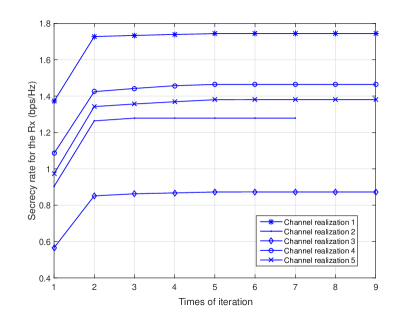
Figure 3: The secrecy rate by CJ-DPS versus the number of iterations for the alternating optimization in Table I with $P_{s}=40$dBm, $N=10$, and $K=5$.

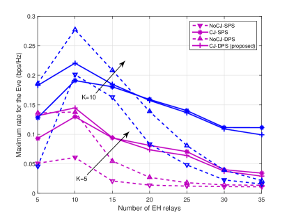
(a) $\max\limits_{k}r_{\rm S,E,k}$ versus the number of relays.

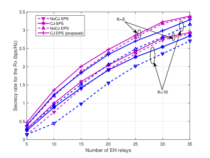
(b) The achievable secrecy rate vs the number of AF relays.

Figure 4: Comparison of different schemes with $P_{s}=10$dB for $K=5$ and $K=10$, respectively.

Fig. 4 shows the achievable secrecy rate for the legitimate Rx with the increase in the number of AF relays by different schemes. As we can see, the secure multi-AF relaying schemes assisted by the transmission of AN outperforms that without AN for both SPS and DPS. In addition, with the increase in $N$, the role of CJ gradually reduces for both schemes of SPS and DPS. This is because as $N$ gets larger, the optimal designs tend to suppress the interception at the most capable eavesdropper more effectively with $N$ DoF, enforcing the numerator of $\max_{k\in\mathcal{K}}{\rm SINR}_{\rm S,E,k}$ to a relatively low level, which can also be observed from $\max_{k\in\mathcal{K}}r_{S,E,k}$ in Fig. 4(a), and therefore the optimal amount of power allocated to AN beams inclines to be little; otherwise the jamming yielded will be detrimental to the reception at the legitimate Rx. Besides, given the same number of AF relays, the secrecy performance gains brought by the proposed schemes with CJ are more prominent in the presence of more eavesdroppers, since it is hard to reduce all the eavesdroppers’ channel capacity without resorting to CJ properly.

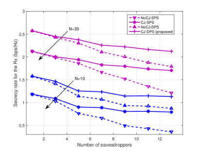
Figure 5: The secrecy rate versus the number of eavesdroppers with $P_{s}=10$dB for $N=10$ and $N=20$, respectively.

Fig. 5 shows the achievable secrecy rate for the legitimate Rx versus the number of eavesdroppers by different schemes. First, similar to the results shown in Fig. 4, the proposed AN-aided multi-AF relaying designs operating with DPS-enabled relays, viz CJ-DPS, perform best among all the schemes. Secondly, as $K$ goes up, the AN-aided schemes, CJ-DPS and CJ-SPS, allow the secrecy rate to drop slowly, in other words, more robust against multiple eavesdroppers, while the secrecy rate of their NoCJ counterparts almost goes down linearly with $K$. Furthermore, with $K$ increasing, for example, more than $10$, the increase in the number of relays, from $N=10$ to $20$, cannot replace the role of CJ as shown in Fig. 4 and 5, since in the presence of many eavesdroppers, more relays may also result in improved eavesdroppers’ decoding ability w/o the assistance of CJ. It is also noteworthy that with $K=1$, there is little use of CJ by the centralized schemes, which was also observed in [36].

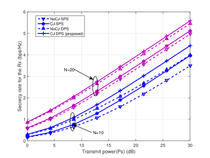
Figure 6: The secrecy rate versus the transmit power with $K=5$ for $N=10$ and $N=20$, respectively.

Fig. 6 provides simulation results of different schemes by varying the source transmit power. It is seen that with more power available at the source, the advantage of CJ is more pronounced, since given other variables fixed, larger $P_{s}$ indicates larger feasible regions for $\mathrm{(P1)}$ and $\mathrm{(P2)}$. Furthermore, as similarly seen in Fig. 4, with a mild number of eavesdroppers ($K=5$), subject to the same $P_{s}$, a large number of cooperative relays enables more DoF in designing the optimal $\alpha_{i}$’s and $\measuredangle\beta_{i}$’s, which alleviates the dependence on AN beams to combat Eves.

VI-B Secrecy Performance by Distributed Algorithms

Here, we study the performance of the distributed schemes, namely, Distributed-SPS and Distributed-DPS in Section V. As mentioned earlier, these heuristics are provided as benchmarks to demonstrate what can be done under the extreme “no-coordination” circumstance, in comparison with Random PS. Note that any other distributed schemes with certain level of cooperation among relays are supposed to increase the secrecy performance up to the proposed centralized algorithms, namely, CJ-DPS and CJ-SPS, at the expense of extra computational complexity and system overhead.

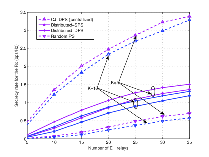
Figure 7: The secrecy rate versus the number of AF relays by distributed algorithms with $P_{s}=10$dB and $K=5$.

Fig. 7 provides the results for the achievable secrecy rate of various schemes versus the number of relays. Distributed-SPS and Distributed-DPS, are observed to be outperformed by their centralized counterparts though, they are considerably superior to Random PS. It is also seen that the performance gap between the centralized and distributed approaches is enlarged as $N$ increases, which is expected, since larger $N$ yields more DoF for cooperation that is exclusively beneficial for the centralized schemes. Furthermore, compared with the centralized schemes, the distributed ones are more vulnerable to the increase in the eavesdroppers’ number.

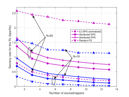
Figure 8: The secrecy rate versus the number of eavesdroppers by distributed algorithms with $P_{s}=10$dB and $N$=8.

In Fig. 8, we investigate the relationship between the secrecy rate performance and the number of eavesdroppers by different methods. As can be observed, compared with the centralized schemes, the secrecy rates achieved by Distributed-SPS and Distributed-DPS both reduce more drastically with the increase in $K$ due to the lack of effective cooperation. Also, the advantage of DPS over SPS for the distributed schemes is compromised since $\alpha_{i}$’s are not jointly designed with other parameters. At last, a similar observation has been made as that for Fig. 7, that is, larger $N$ yields more visible performance gap between the centralized and distributed approaches.

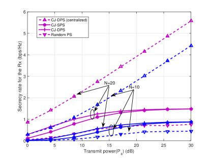
Figure 9: The secrecy rate versus transmit power by distributed algorithms with $N=10$ and $K=5$.

In Fig. 9, we examine the effect of increasing the transmit power at the source on the secrecy performance of different schemes under the same settings as those in Fig. 6. Among all the presented designs, CJ-DPS still achieves the best secrecy rate as observed in other examples. Also, the fact that larger $N$ benefits more from cooperative designs is corroborated again due to the same reason as that for Fig. 7 and 8. Furthermore, the secrecy rate of Distributed-SPS or Distributed-DPS is quickly saturated when $P_{s}>20$dB while that for their centralized counterparts still rises at fast speed.

VII conclusion

This paper studied secure communications using multiple single-antenna WEH-enabled AF relays assisted by AN via CJ for a SWIPT network with multiple single-antenna eavesdroppers. Using PS at the relays, the achievable secrecy rates for the relay wiretap channel were maximized by jointly optimizing the CB and the CJ covariance matrix along with the PS ratios for relays operating with, respectively, SPS and DPS. For DPS, Reformulating the constraints into restricted hyperbolic forms enabled us to develop convex optimization-based solutions. Further, we proposed an information-exchange-free distributed algorithm that outperforms the random decision.

-A Proof of Lemma IV.1

As the optimal solution to $\mathrm{(P1.1\text{-}SDP)}$ is proved to be optimal to problem $\mathrm{(P1.1)}$, the optimum value for $\mathrm{(P1.1\text{-}SDP)}$ is $\tau f_{1}(\tau)=H_{1}(\tau)$. Hence, we identify the property of $H_{1}(\tau)$ by investigating $\mathrm{(P1.1\text{-}SDP)}$, with its Lagrangian given by

$$\mathcal{L}(\chi)= {\rm trace}\left(\left(\begin{array}[]{r}P_{s}\tilde{\boldsymbol{h}}_{sd}^{\dagger}\tilde{\boldsymbol{h}}_{sd}^{T}-\lambda\boldsymbol{D}_{\hat{sd}}\\ +\sum_{k=1}^{K}\theta_{k}\left(\frac{1}{\tau}-1\right)\boldsymbol{D}_{\hat{se},k}\\ -\sum_{k=1}^{K}\theta_{k}P_{s}\tilde{\boldsymbol{h}}_{se,k}^{\dagger}\tilde{\boldsymbol{h}}_{se,k}^{T}\\ -\boldsymbol{W}_{0}^{\tfrac{1}{2}}\boldsymbol{U}\boldsymbol{W}_{0}^{\tfrac{1}{2}}+\boldsymbol{Y}_{1}\end{array}\right)\hat{\boldsymbol{X}}_{1}\right)+{\rm trace}\left(\left(\begin{array}[]{r}-\lambda\boldsymbol{h}_{rd}^{\dagger}\boldsymbol{h}_{rd}^{T}\\ +\sum_{k=1}^{K}\theta_{k}\left(\frac{1}{\tau}-1\right)\boldsymbol{h}_{re,k}^{\dagger}\boldsymbol{h}_{re,k}^{T}\\ -\boldsymbol{U}+\boldsymbol{Y}_{2}\end{array}\right)\hat{\boldsymbol{S}}\right)$$ (62)

$$+\left(\begin{array}[]{r}-\lambda\sigma_{n_{d}}^{2}+\sum_{k=1}^{K}\theta_{k}\left(\frac{1}{\tau}-1\right)\sigma_{n_{e},k}^{2}\\ +{\rm trace}\left(\boldsymbol{W}_{0}^{\frac{1}{2}}\boldsymbol{U}\boldsymbol{W}_{0}^{\frac{1}{2}}\right)+\zeta\end{array}\right)\xi+\lambda\tau,$$ (65)

where $\chi$ denotes a tuple consisting of all the primal and dual variables. Specifically, $\boldsymbol{Y}_{1}$, $\boldsymbol{Y}_{2}$ and $\lambda$ are Lagrangian multipliers associated with $\hat{\boldsymbol{X}}_{1}$, $\hat{\boldsymbol{S}}$ and the first constraint of $\mathrm{(P1.1\text{-}SDP)}$, respectively; $\{\theta_{k}\}$ are the dual variables associated with the SINR constraint for the $k$th Eve, respectively; $\boldsymbol{U}={\rm diag}([u_{i}]_{i=1}^{N})$ with each diagonal entry $u_{i}$ denoting the dual variable associated with the per-relay power constraint; $\zeta$ is the Lagrangian multiplier associated with $\xi\geq 0$. In addition, $\boldsymbol{W}_{0}={\rm diag}([\eta\bar{\alpha}_{i}P_{s}|h_{sr_{i}}|^{2}]_{i=1}^{N})$. The Karush-Kuhn-Tucker (KKT) conditions for (65) are partially listed as follows:

$$\boldsymbol{Y}_{1}=-P_{s}\tilde{\boldsymbol{h}}_{sd}^{\dagger}\tilde{\boldsymbol{h}}_{sd}^{T}+\lambda\boldsymbol{D}_{\hat{sd}}-\sum_{k=1}^{K}\theta_{k}\left(\frac{1}{\tau}-1\right)\boldsymbol{D}_{\hat{se},k}+\sum_{k=1}^{K}\theta_{k}P_{s}\tilde{\boldsymbol{h}}_{se,k}^{\dagger}\tilde{\boldsymbol{h}}_{se,k}^{T}+\boldsymbol{W}_{0}^{\frac{1}{2}}\boldsymbol{U}\boldsymbol{W}_{0}^{\frac{1}{2}},$$ (66a)

$$\boldsymbol{Y}_{2}=\lambda\boldsymbol{h}_{rd}^{\dagger}\boldsymbol{h}_{rd}^{T}-\sum_{k=1}^{K}\theta_{k}\left(\frac{1}{\tau}-1\right)\boldsymbol{h}_{re,k}^{\dagger}\boldsymbol{h}_{re,k}^{T}+\boldsymbol{U},$$ (66b)

$$\zeta=\lambda\sigma_{n_{d}}^{2}-\sum_{k=1}^{K}\theta_{k}\left(\frac{1}{\tau}-1\right)\sigma_{n_{e},k}^{2}-{\rm trace}(\boldsymbol{W}_{0}^{\frac{1}{2}}\boldsymbol{U}\boldsymbol{W}_{0}^{\frac{1}{2}}).$$ (66c)

The associated dual problem is accordingly given by

$$\mathrm{(P1.1\text{-}SDP}\mathrm{\text{-}dual)}:$$

$$\left\{\begin{aligned} \min_{\lambda,\{\theta_{k}\},\{u_{i}\}}&~{}\lambda\tau\\ {\rm s.t.}&~{}\theta_{k}\geq 0,\;\forall k,\ u_{i}\geq 0,\;\forall i,\\ &~{}\lambda\geq 0,\ \zeta\geq 0,\ \boldsymbol{Y}_{1}\succeq\boldsymbol{0},\ \boldsymbol{Y}_{2}\succeq\boldsymbol{0},\end{aligned}\right.$$

where $\boldsymbol{Y}_{1}$, $\boldsymbol{Y}_{2}$, and $\zeta$ are given by (66a)–(66c), respectively. Since it is easily verified that $\mathrm{(P1.1\text{-}SDP)}$ satisfies the Slater condition, the strong duality holds [33]. This implies that the dual optimum value in $\mathrm{(P1.1\text{-}SDP\text{-}dual)}$ is $H_{1}(\tau)$, which turns out to be a point-wise minimum of a family of affine functions and thus concave over $\tau\in[\tau_{\min,1},1]$ [33, pp. 80].

-B Proof of Proposition IV.1

The KKT conditions for (65) yield the following complementary slackness:

$$\boldsymbol{Y}_{1}\hat{\boldsymbol{X}}_{1}^{\ast}=\boldsymbol{0},$$ (67a)

$$\boldsymbol{Y}_{2}\hat{\boldsymbol{S}}^{\ast}=\boldsymbol{0}.$$ (67b)

Pre- and post-multiplying $\boldsymbol{W}_{0}^{\frac{1}{2}}$ with the left hand side (LHS) and right hand side (RHS) of (66b), respectively, and substituting $\boldsymbol{W}_{0}^{\frac{1}{2}}\boldsymbol{U}^{\ast}\boldsymbol{W}_{0}^{\frac{1}{2}}$ into (66a), $\boldsymbol{Y}_{1}^{\ast}$ can be rewritten as

$$\boldsymbol{Y}_{1}= -P_{s}\tilde{\boldsymbol{h}}_{sd}^{\dagger}\tilde{\boldsymbol{h}}_{sd}^{T}+\lambda\boldsymbol{D}_{\hat{sd}}-\sum_{k=1}^{K}\theta_{k}\left(\frac{1}{\tau}-1\right)\boldsymbol{D}_{\hat{se},k}-\lambda\boldsymbol{W}_{0}^{\frac{1}{2}}\boldsymbol{h}_{rd}^{\dagger}\boldsymbol{h}_{rd}^{T}\boldsymbol{W}_{0}^{\frac{1}{2}}+\sum_{k=1}^{K}\theta_{k}P_{s}\tilde{\boldsymbol{h}}_{se,k}^{\dagger}\tilde{\boldsymbol{h}}_{se,k}^{T}$$

$$+\boldsymbol{W}_{0}^{\frac{1}{2}}\boldsymbol{Y}_{2}\boldsymbol{W}_{0}^{\frac{1}{2}}+\sum_{k=1}^{K}\theta_{k}\left(\frac{1}{\tau}-1\right)\boldsymbol{W}_{0}^{\frac{1}{2}}\boldsymbol{h}_{re,k}^{\dagger}\boldsymbol{h}_{re,k}^{T}\boldsymbol{W}_{0}^{\frac{1}{2}}.$$ (68)

Introducing the notation of $[\cdot]_{\rm offd}$ to represent a square matrix with its diagonal entries removed, it follows from (66b) that

$$\left[\begin{array}[]{r}\boldsymbol{W}_{0}^{\frac{1}{2}}\boldsymbol{Y}_{2}\boldsymbol{W}_{0}^{\frac{1}{2}}-\lambda\boldsymbol{W}_{0}^{\frac{1}{2}}\boldsymbol{h}_{rd}^{\dagger}\boldsymbol{h}_{rd}^{T}\boldsymbol{W}_{0}^{\frac{1}{2}}\\ -\sum_{k=1}^{K}\theta_{k}\left(\frac{1}{\tau}-1\right)\boldsymbol{W}_{0}^{\frac{1}{2}}\boldsymbol{h}_{re,k}^{\dagger}\boldsymbol{h}_{re,k}^{T}\boldsymbol{W}_{0}^{\frac{1}{2}}\end{array}\right]_{\rm offd}=\boldsymbol{0}.$$ (69)

By subtracting (69) from (-B), $\boldsymbol{Y}_{1}$ can be rewritten as

$$\boldsymbol{Y}_{1}= -P_{s}\tilde{\boldsymbol{h}}_{sd}^{\dagger}\tilde{\boldsymbol{h}}_{sd}^{T}+\lambda\boldsymbol{D}_{\hat{sd}}-\sum_{k=1}^{K}\theta_{k}\left(\frac{1}{\tau}-1\right)\boldsymbol{D}_{\hat{se},k}-\left[\begin{array}[]{r}\lambda\boldsymbol{W}_{0}^{\frac{1}{2}}\boldsymbol{h}_{rd}^{\dagger}\boldsymbol{h}_{rd}^{T}\boldsymbol{W}_{0}^{\frac{1}{2}}\\ -\sum_{k=1}^{K}\theta_{k}\left(\frac{1}{\tau}-1\right)\boldsymbol{W}_{0}^{\frac{1}{2}}\boldsymbol{h}_{re,k}^{\dagger}\boldsymbol{h}_{re,k}^{T}\boldsymbol{W}_{0}^{\frac{1}{2}}\end{array}\right]_{\rm d}$$ (72)

$$+\left[\boldsymbol{W}_{0}^{\frac{1}{2}}\boldsymbol{Y}_{2}\boldsymbol{W}_{0}^{\frac{1}{2}}\right]_{\rm d}+\sum_{k=1}^{K}\theta_{k}P_{s}\tilde{\boldsymbol{h}}_{se,k}^{\dagger}\tilde{\boldsymbol{h}}_{se,k}^{T},$$ (73)

where $[\cdot]_{\rm d}$ denotes a square matrix with only the diagonal remained. Observing that

$$\!\!(\boldsymbol{D}_{\hat{sd}})^{-1}\boldsymbol{D}_{\hat{se}} =\left[\boldsymbol{W}_{0}^{\frac{1}{2}}\boldsymbol{h}_{rd}^{\dagger}\boldsymbol{h}_{rd}^{T}\boldsymbol{W}_{0}^{\frac{1}{2}}\right]_{\rm d}^{-1}\left[\boldsymbol{W}_{0}^{\frac{1}{2}}\boldsymbol{h}_{re,k}^{\dagger}\boldsymbol{h}_{re,k}^{T}\boldsymbol{W}_{0}^{\frac{1}{2}}\right]_{\rm d}$$

$$={\rm diag}\left([|h_{r_{i}e,k}|^{2}\left.\middle/\right.|h_{r_{i}d}|^{2}]_{i=1}^{N}\right)$$

$$\equiv\boldsymbol{R}_{ed,k},$$ (74)

$\boldsymbol{Y}_{1}^{\ast}$ can be finally recast as

$$\boldsymbol{Y}_{1}^{\ast}=-P_{s}\tilde{\boldsymbol{h}}_{sd}^{\dagger}\tilde{\boldsymbol{h}}_{sd}^{T}+\boldsymbol{\Xi}+\sum_{k=1}^{K}\theta_{k}P_{s}\tilde{\boldsymbol{h}}_{se,k}^{\dagger}\tilde{\boldsymbol{h}}_{se,k}^{T},$$ (75)

where

$$\boldsymbol{\Xi}=\left[\boldsymbol{W}_{0}^{\frac{1}{2}}\boldsymbol{Y}_{2}\boldsymbol{W}_{0}^{\frac{1}{2}}\right]_{\rm d}-\left(\left[\boldsymbol{W}_{0}^{\frac{1}{2}}\boldsymbol{h}_{rd}^{\dagger}\boldsymbol{h}_{rd}^{T}\boldsymbol{W}_{0}^{\frac{1}{2}}\right]_{\rm d}-\boldsymbol{D}_{\hat{sd}}\right)\left(\lambda\boldsymbol{I}-\sum_{k=1}^{K}\theta_{k}\left(\frac{1}{\tau}-1\right)\boldsymbol{R}_{ed,k}\right).$$ (76)

In the following, we show that $\boldsymbol{\Xi}+\sum_{k=1}^{K}\theta_{k}P_{s}\tilde{\boldsymbol{h}}_{se,k}^{\dagger}\tilde{\boldsymbol{h}}_{se,k}^{T}$ is a positive definite matrix. Note that since $\boldsymbol{\Xi}$ is a diagonal matrix, its definiteness is only determined by the signs of its diagonal entries, for which we commence with the discussion in three difference cases below.

1. Case I: $\exists i$ such that $\lambda-\sum_{k=1}^{K}\theta_{k}\left(\frac{1}{\tau}-1\right)[\boldsymbol{R}_{ed,k}]_{i,i}<0$. Since $\left[\left[\boldsymbol{W}_{0}^{\frac{1}{2}}\boldsymbol{h}_{rd}^{\dagger}\boldsymbol{h}_{rd}^{T}\boldsymbol{W}_{0}^{\frac{1}{2}}\right]_{\rm d}-\boldsymbol{D}_{\hat{sd}}\right]_{i,i}=$
   $\eta\bar{\alpha}_{i}P_{s}|h_{sr_{i}}|^{2}|h_{r_{i}d}|^{2}\left(1-\frac{(1-\bar{\alpha}_{i})\sigma_{n_{a}}^{2}+\sigma_{n_{c}}^{2}}{(1-\bar{\alpha}_{i})(|h_{sr_{i}}|^{2}P_{s}+\sigma_{n_{a}}^{2})+\sigma_{n_{c}}^{2}}\right)>0$, it follows from (76) that $[\boldsymbol{\Xi}]_{i,i}>0$ in this case.

2. Case II: $\exists i$ such that $\lambda-\sum_{k=1}^{K}\theta_{k}\left(\frac{1}{\tau}-1\right)[\boldsymbol{R}_{ed,k}]_{i,i}>0$. We have $\left[\left[\boldsymbol{W}_{0}^{\frac{1}{2}}\boldsymbol{Y}_{2}\boldsymbol{W}_{0}^{\frac{1}{2}}\right]_{\rm d}\right]_{i,i}-[\boldsymbol{W}_{0}]_{i,i}|h_{r_{i}d}|^{2}(\lambda^{\ast}-\sum_{k=1}^{K}\theta_{k}\left(\frac{1}{\tau}-1\right)[\boldsymbol{R}_{ed,k}]_{i,i})\geq 0$ in accordance with (66b), which implies that $[\boldsymbol{\Xi}]_{i,i}=\left[\left[\boldsymbol{W}_{0}^{\frac{1}{2}}\boldsymbol{Y}_{2}\boldsymbol{W}_{0}^{\frac{1}{2}}\right]_{\rm d}\right]_{i,i}-[\boldsymbol{W}_{0}]_{i,i}|h_{r_{i}d}|^{2}(\lambda-\sum_{k=1}^{K}\theta_{k}\left(\frac{1}{\tau}-1\right)[\boldsymbol{R}_{ed,k}]_{i,i})+[\boldsymbol{D}_{\hat{sd}}]_{i,i}(\lambda-\sum_{k=1}^{K}\theta_{k}\left(\frac{1}{\tau}-1\right)[\boldsymbol{R}_{ed,k}]_{i,i})>0$ (c.f. (76)).

3. Case III: $\exists i$ such that $\lambda-\sum_{k=1}^{K}\theta_{k}\left(\frac{1}{\tau}-1\right)[\boldsymbol{R}_{ed,k}]_{i,i}=0$. In this case, it follows that $[\boldsymbol{\Xi}]_{i,i}=\left[\boldsymbol{W}_{0}^{\frac{1}{2}}\boldsymbol{Y}_{2}\boldsymbol{W}_{0}^{\frac{1}{2}}\right]_{i,i}$
   $\geq 0$. It is noteworthy that the number of $i$’s such that $\lambda-\sum_{k=1}^{K}\theta_{k}\left(\frac{1}{\tau}-1\right)[\boldsymbol{R}_{ed,k}]_{i,i}=0$ cannot exceed one. This can be proved by contradiction as follows. If $\exists i_{1},i_{2}$, $i_{1}\neq i_{2}$, such that $\lambda-\sum_{k=1}^{K}\theta_{k}\left(\frac{1}{\tau}-1\right)[\boldsymbol{R}_{ed,k}]_{i_{1},i_{1}}=0$ and $\lambda-\sum_{k=1}^{K}\theta_{k}\left(\frac{1}{\tau}-1\right)[\boldsymbol{R}_{ed,k}]_{i_{2},i_{2}}=0$, it implies that $\sum_{k=1}^{K}\theta_{k}[\boldsymbol{R}_{ed,k}]_{i_{1},i_{1}}=\sum_{k=1}^{K}\theta_{k}[\boldsymbol{R}_{ed,k}]_{i_{2},i_{2}}$, which contradicts to the fact that for any two independent continuously distributed random variables, the chance that they are equal is zero.

In summary, $[\boldsymbol{\Xi}]_{i,i}\geq 0$, $\forall i$. If $[\boldsymbol{\Xi}]_{i,i}>0$, then it is obvious that $\boldsymbol{\Xi}+\sum_{k=1}^{K}\theta_{k}P_{s}\tilde{\boldsymbol{h}}_{se,k}^{\dagger}\tilde{\boldsymbol{h}}_{se,k}^{T}\succ\boldsymbol{0}$. Next, we show that it still holds true in the case that $\exists i^{\prime}$, such that $[\boldsymbol{\Xi}]_{i^{\prime},i^{\prime}}=0$, $i^{\prime}\in\mathcal{N}$, by definition. Define the null-space of $\boldsymbol{\Xi}$ by $\psi=\{\boldsymbol{\eta}|\boldsymbol{\eta}=\alpha\boldsymbol{e}_{i^{\prime}},\alpha\in\mathbb{C}\}$ and multiply $\boldsymbol{\eta}^{H}$ and $\boldsymbol{\eta}$, $\forall\boldsymbol{\eta}\neq\boldsymbol{0}$, on the LHS and RHS of $\boldsymbol{\Xi}+\sum_{k=1}^{K}\theta_{k}P_{s}\tilde{\boldsymbol{h}}_{se,k}^{\dagger}\tilde{\boldsymbol{h}}_{se,k}^{T}$, respectively. If $\boldsymbol{\eta}\notin\psi$, it is straightforward to obtain $\boldsymbol{\eta}^{H}(\boldsymbol{\Xi}+\sum_{k=1}^{K}\theta_{k}P_{s}\tilde{\boldsymbol{h}}_{se,k}^{\dagger}\tilde{\boldsymbol{h}}_{se,k}^{T})\boldsymbol{\eta}>0$; otherwise, it follows that $\boldsymbol{\eta}^{H}(\boldsymbol{\Xi}+\sum_{k=1}^{K}\theta_{k}P_{s}\tilde{\boldsymbol{h}}_{se,k}^{\dagger}\tilde{\boldsymbol{h}}_{se,k}^{T})\boldsymbol{\eta}=\sum_{k=1}^{K}\theta_{k}P_{s}\alpha^{2}|[\tilde{\boldsymbol{h}}_{se,k}]_{i^{\prime}}|^{2}>0$, as $[\tilde{\boldsymbol{h}}_{se,k}]_{i^{\prime}}\neq 0$ in probability. This completes the proof. As a result, $\boldsymbol{Y}_{1}$ in (75) is shown to always take on a special structure, that is, a full-rank matrix minus a rank-one matrix. Note that this observation plays a key role in proving the rank-one property of $\hat{\boldsymbol{X}}_{1}^{\ast}$, which is also identified in [20, Appendix C].

$$\left\|\begin{array}[]{c}2\sigma_{n_{c}}{\rm trace}(\boldsymbol{U}_{2}\boldsymbol{E}_{i})\\ 2\sqrt{\left(1-\frac{\bar{z}_{i}}{c_{0,i}}\right)\frac{1}{c_{1,i}}}\\ \left(1-\frac{\bar{z}_{i}}{c_{0,i}}-c_{1,i}{\rm trace}(\boldsymbol{U}_{1}\boldsymbol{E}_{i})\right)-\left({\rm trace}(\boldsymbol{U}_{2}\boldsymbol{E}_{i})+\frac{1}{c_{1,i}}\right)\end{array}\right\| \leq\left(1-\frac{\bar{z}_{i}}{c_{0,i}}-c_{1,i}x_{i}\right)+\left(y_{i}+\frac{1}{c_{1,i}}\right)$$ (80)

$$\left\|\begin{array}[]{c}2\sigma_{n_{c}}{\rm trace}(\boldsymbol{U}_{2}\boldsymbol{E}_{i})\\ 2\sqrt{\frac{1}{c_{1,i}}}\\ \left(1-c_{1,i}{\rm trace}(\boldsymbol{U}_{1}\boldsymbol{E}_{i})\right)-\left({\rm trace}(\boldsymbol{U}_{2}\boldsymbol{E}_{i})+\frac{1}{c_{1,i}}\right)\end{array}\right\| \leq\left(1-c_{1,i}x_{i}\right)+\left(y_{i}+\frac{1}{c_{1,i}}\right)$$ (84)

Finally, multiplying both sides of (75) by $\hat{\boldsymbol{X}}_{1}^{\ast}$, as per (67a), we obtain the following equation:

$$\hat{\boldsymbol{X}}_{1}^{\ast}=P_{s}\left(\boldsymbol{\Xi}+\sum_{k=1}^{K}\theta_{k}P_{s}\tilde{\boldsymbol{h}}_{se,k}^{\dagger}\tilde{\boldsymbol{h}}_{se,k}^{T}\right)^{-1}\tilde{\boldsymbol{h}}_{sd}^{\dagger}\tilde{\boldsymbol{h}}_{sd}^{T}\hat{\boldsymbol{X}}_{1}^{\ast},$$ (85)

which further implies that ${\rm rank}(\hat{\boldsymbol{X}}_{1}^{\ast})\leq{\rm rank}(\tilde{\boldsymbol{h}}_{sd}^{\dagger}\tilde{\boldsymbol{h}}_{sd}^{T})=1$. In addition, since the optimality of $\mathrm{(P1.1\text{-}SDP)}$ suggests that $\hat{\boldsymbol{X}}_{1}^{\ast}\neq\boldsymbol{0}$, ${\rm rank}(\hat{\boldsymbol{X}}_{1}^{\ast})=1$ is thus proved.

As $\hat{\boldsymbol{X}}_{1}^{\ast}$ can be decomposed as $\hat{\boldsymbol{w}}_{1}^{\ast}\hat{\boldsymbol{w}}_{1}^{\ast H}$ by EVD, (67a) results in $\boldsymbol{Y}_{1}\hat{\boldsymbol{w}}_{1}^{\ast}=\boldsymbol{0}$, which further implies that

$$\hat{\boldsymbol{w}}_{1}^{\ast}=P_{s}\left(\boldsymbol{\Xi}+\sum_{k=1}^{K}\theta_{k}P_{s}\tilde{\boldsymbol{h}}_{se,k}^{\dagger}\tilde{\boldsymbol{h}}_{se,k}^{T}\right)^{-1}\tilde{\boldsymbol{h}}_{sd}^{\dagger}\tilde{\boldsymbol{h}}_{sd}^{T}\hat{\boldsymbol{w}}_{1}^{\ast}.$$ (86)

Therefore, (86) admits a unique solution $\hat{\boldsymbol{w}}_{1}$ up to a scaling factor, which is given by

$$\hat{\boldsymbol{w}}_{1}=\left(\boldsymbol{\Xi}+\sum_{k=1}^{K}\theta_{k}P_{s}\tilde{\boldsymbol{h}}_{se,k}^{\dagger}\tilde{\boldsymbol{h}}_{se,k}^{T}\right)^{-1}\tilde{\boldsymbol{h}}_{sd}^{\dagger}.$$ (87)

Consequently, we have $\hat{\boldsymbol{w}}_{1}^{\ast}=\beta\hat{\boldsymbol{w}}_{1}$, where $\beta\in\mathbb{R}_{+}$. On the other hand, by plugging $\hat{\boldsymbol{w}}_{1}^{\ast}=\beta\hat{\boldsymbol{w}}_{1}$ into the equality constraint of $\mathrm{(P1.1\text{-}SDP)}$, we have $\beta=\sqrt{\frac{\tau-\xi^{\ast}\sigma_{n_{d}}^{2}-{\rm trace}(\hat{\boldsymbol{S}}^{\ast}\boldsymbol{h}_{rd}^{\dagger}\boldsymbol{h}_{rd}^{T})}{{\rm trace}(\hat{\boldsymbol{w}}_{1}\hat{\boldsymbol{w}}_{1}^{H}\boldsymbol{D}_{\hat{sd}})}}$, which yields

$$\hat{\boldsymbol{w}}_{1}^{\ast}=\sqrt{\frac{\tau-\xi^{\ast}\sigma_{n_{d}}^{2}-{\rm trace}(\hat{\boldsymbol{S}}^{\ast}\boldsymbol{h}_{rd}^{\dagger}\boldsymbol{h}_{rd}^{T})}{{\rm trace}(\hat{\boldsymbol{w}}_{1}\hat{\boldsymbol{w}}_{1}^{H}\boldsymbol{D}_{\hat{sd}})}}\hat{\boldsymbol{w}}_{1}.$$ (88)

At last, we show $3)$ of Proposition IV.1. For the case of $K\geq N$, it is obvious that ${\rm rank}(\hat{\boldsymbol{S}})^{\ast}\leq N$. For the case of $K<N$, only a sketch of the proof is provided here due to the length constraint. According to (66b), first it is provable that $\lambda\boldsymbol{h}_{rd}^{\dagger}\boldsymbol{h}_{rd}^{T}+\boldsymbol{U}$ is a full-rank matrix when $\mathrm{(P1.1\text{-}SDP)}$ obtains its optimum value; next, observing that ${\rm rank}(\boldsymbol{Y}_{2})\geq N-{\rm rank}(\sum_{k=1}^{K}\theta_{k}\boldsymbol{h}_{re,k}^{\dagger}\boldsymbol{h}_{re,k}^{T})$, it follows that ${\rm rank}(\boldsymbol{Y}_{2})\geq N-K$ as a result of ${\rm rank}(\sum_{k=1}^{K}\theta_{k}\boldsymbol{h}_{re,k}^{\dagger}\boldsymbol{h}_{re,k}^{T})\leq K$; then according to (67b), ${\rm rank}(\hat{\boldsymbol{S}}^{\ast})\leq K$ is thus obtained.

-C Proof of Proposition IV.2

First, use the following lemma to rewrite $\mathrm{(P2^{\prime}.1\text{-}SDR)}$.

Lemma .1

Problem $\mathrm{(P2^{\prime}.1\text{-}SDR)}$ is equivalent to the following problem:

$$~{}\mathrm{(P2^{\prime}.1\text{-}SDR\text{-}Eqv)}:$$

$$\left\{\begin{aligned} &\max_{\boldsymbol{U}_{1},\boldsymbol{U}_{2},\{x_{i}\},\{y_{i}\}}~{}\eqref{eq:obj for (P2'.1-SDR)}\\ &\mathtt{s.t.}~{}\eqref{eq:SINR constraint for (P2'.1-SDR)},\;\forall k,\;\eqref{eq:equivalent SOC per-relay jamming constraint},\,\eqref{eq:equivalent SOC constraint on rho},\;\forall i,\\ &{\rm trace}(\boldsymbol{U}_{1}\boldsymbol{E}_{i})\leq x_{i},\,{\rm trace}(\boldsymbol{U}_{2}\boldsymbol{E}_{i})\geq y_{i},\;\forall i,\\ &{\rm trace}((\boldsymbol{U}_{1}-\boldsymbol{U}_{2})\boldsymbol{E}_{i})\leq 0,\;\forall i,\\ &\boldsymbol{U}_{1}\succeq\boldsymbol{0},\ \boldsymbol{U}_{2}\succeq\boldsymbol{0},\end{aligned}\right.$$

where (80) and (84) are given at the top of next page.

Proof:

For convenience of the proof, the optimum value for $\mathrm{(P2^{\prime}.1\text{-}SDR)}$ and $\mathrm{(P2^{\prime}.1\text{-}SDR\text{-}Eqv)}$ are denoted by $f_{0}^{\ast}$ and $\tilde{f}_{0}^{\ast}$, respectively. Assuming that $(\boldsymbol{U}_{1}^{\ast},\boldsymbol{U}_{2}^{\ast},\{x_{i}^{\ast}\},\{y_{i}^{\ast}\})$ is the optimal solution to $\mathrm{(P2^{\prime}.1\text{-}SDR)}$, it is easily verified to be feasible for $\mathrm{(P2^{\prime}.1\text{-}SDR\text{-}Eqv)}$ as well, which implies that $f_{0}^{\ast}\leq\tilde{f}_{0}^{\ast}$. On the other hand, if $\mathrm{(P2^{\prime}.1\text{-}SDR\text{-}Eqv)}$ returns an optimal solution of $(\tilde{\boldsymbol{U}}_{1}^{\ast},\tilde{\boldsymbol{U}}_{2}^{\ast},\{\tilde{x}_{i}^{\ast}\},\{\tilde{y}_{i}^{\ast}\})$, by defining ${\rm trace}(\tilde{\boldsymbol{U}}_{1}^{\ast}\boldsymbol{E}_{i})=x_{i}^{\prime\ast}$ and ${\rm trace}(\tilde{\boldsymbol{U}}_{2}^{\ast}\boldsymbol{E}_{i})=y_{i}^{\prime\ast}$, $\forall i$, we show that $(\tilde{\boldsymbol{U}}_{1}^{\ast},\tilde{\boldsymbol{U}}_{2}^{\ast},\{x_{i}^{\prime\ast}\},\{y_{i}^{\prime\ast}\})$ is also feasible for $\mathrm{(P2^{\prime}.1\text{-}SDR)}$ as follows. As for (40),

$$\left\|\begin{array}[]{c}2\sigma_{n_{c}}y_{i}^{\prime\ast}\\ 2\sqrt{\left(1-\frac{\bar{z}_{i}}{c_{0,i}}\right)\tfrac{1}{c_{1,i}}}\\ \left(1-\frac{\bar{z}_{i}}{c_{0,i}}-c_{1,i}x_{i}^{\prime\ast}\right)-\left(y_{i}^{\prime\ast}+\frac{1}{c_{1,i}}\right)\end{array}\right\|$$ (92)

$$\stackrel{{\scriptstyle(a)}}{{\leq}}\left(1-\frac{\bar{z}_{i}}{c_{0,i}}-c_{1,i}\tilde{x}_{i}^{\ast}\right)+\left(\tilde{y}_{i}^{\ast}+\frac{1}{c_{1,i}}\right)$$

$$\stackrel{{\scriptstyle(b)}}{{\leq}}\left(1-\tfrac{\bar{z}_{i}}{c_{0,i}}-c_{1,i}{\rm trace}(\tilde{\boldsymbol{U}}_{1}^{\ast}\boldsymbol{E}_{i})\right)+\left({\rm trace}(\tilde{\boldsymbol{U}}_{2}^{\ast}\boldsymbol{E}_{i})+\tfrac{1}{c_{1,i}}\right)$$

$$=\left(1-\frac{\bar{z}_{i}}{c_{0,i}}-c_{1,i}x_{i}^{\prime\ast}\right)+\left(y_{i}^{\prime\ast}+\frac{1}{c_{1,i}}\right),$$ (93)

where $(a)$ is due to (80), and $(b)$ comes from ${\rm trace}(\tilde{\boldsymbol{U}}_{1}^{\ast}\boldsymbol{E}_{i})\leq\tilde{x}_{i}^{\ast}$ and ${\rm trace}(\tilde{\boldsymbol{U}}_{2}^{\ast}\boldsymbol{E}_{i})\geq\tilde{y}_{i}^{\ast}$. Similarly, $(\tilde{\boldsymbol{U}}_{1}^{\ast},\tilde{\boldsymbol{U}}_{2}^{\ast},\{x_{i}^{\prime\ast}\},$
$\{y_{i}^{\prime\ast}\})$ can be proved to satisfy (45) as well. In addition, $x_{i}^{\prime\ast}-y_{i}^{\prime\ast}={\rm trace}(\tilde{\boldsymbol{U}}_{1}^{\ast}\boldsymbol{E}_{i})-{\rm trace}(\tilde{\boldsymbol{U}}_{2}^{\ast}\boldsymbol{E}_{i})\leq 0$, $\forall i$, i.e., (46) holds true. These feasibility implies that $\tilde{f}_{0}^{\ast}\leq f_{0}^{\ast}$. By combining the above two facts, we have $\tilde{f}_{0}^{\ast}=f_{0}^{\ast}$ and complete the proof. ∎

Then, we apply the Charnes-Cooper transformation again to $\mathrm{(P2^{\prime}.1\text{-}SDR\text{-}Eqv)}$, the result of which is denoted by $\mathrm{(P2^{\prime}.1\text{-}SDP\text{-}Eqv)}$, to study the property of $\hat{\boldsymbol{U}}_{1}^{\ast}$ and $\hat{\boldsymbol{U}}_{2}^{\ast}$. It is noteworthy that the Charnes-Cooper transformed constraint of (80) admits the form given by $\|\boldsymbol{x}^{(i)}\|\leq h(\hat{x}_{i},\hat{y}_{i})$, $\forall i$, where $\boldsymbol{x}^{(i)}$ is the column vector inside $\|\cdot\|$ of the LHS of (80) and $h(\hat{x}_{i},\hat{y}_{i})$ indicates the RHS expression. Since it is easily checked that $\xi>0$ as a result of feasibility, we have $\|\boldsymbol{x}^{(i)}\|>0\Rightarrow h(\hat{x}_{i},\hat{y}_{i})>0$, which implies that

$$\begin{bmatrix}h(\hat{x}_{i},\hat{y}_{i})&\boldsymbol{x}^{(i)^{H}}\\ \boldsymbol{x}^{(i)}&h(\hat{x}_{i},\hat{y}_{i})\boldsymbol{I}\end{bmatrix}\succeq\boldsymbol{0}$$ (94)

according to Schur complement. It thus follows that (94) holds true, $\forall\boldsymbol{x}^{(i)}$: $\|\boldsymbol{x}^{(i)}\|\leq h(\hat{x}_{i},\hat{y}_{i})$. As such, we can show that (80) can be recast into a constraint without $\boldsymbol{x}$, i.e., not related to $\hat{\boldsymbol{U}}_{1}$, $\hat{\boldsymbol{U}}_{2}$, following the same procedure as [37, Appendix III] by exploiting [38, Lemma 2]. Similarly, the Charnes-Cooper transformed constraint of (84) can also be rewritten without $\hat{\boldsymbol{U}}_{1}$, $\hat{\boldsymbol{U}}_{2}$. Hence, the partial Lagrangian for $\mathrm{(P2^{\prime}.1\text{-}SDP\text{-}Eqv)}$ in terms of $\hat{\boldsymbol{U}}_{1}$ and $\hat{\boldsymbol{U}}_{2}$ can be expressed as (95) (see top of next page),

$$\mathcal{L}(\varphi)={\rm trace}\left(\left(\begin{array}[]{r}P_{s}\boldsymbol{s}_{sd}^{\dagger}\boldsymbol{s}_{sd}^{T}-\lambda\sigma_{n_{a}}^{2}{\rm diag}(\boldsymbol{c}_{0}\circ\|\boldsymbol{h}_{rd}\|.^{2})\\ +\sum_{k=1}^{K}\theta_{k}\left(\frac{1}{\tau}-1\right)\sigma_{n_{a}}^{2}{\rm diag}(\boldsymbol{c}_{0}\circ\|\boldsymbol{h}_{re,k}\|.^{2})\\ -P_{s}\sum_{k=1}^{K}\theta_{k}\boldsymbol{s}_{se,k}^{\dagger}\boldsymbol{s}_{se,k}^{T}-\boldsymbol{\Delta}-\boldsymbol{\Sigma}+\boldsymbol{Y}_{1}\end{array}\right)\hat{\boldsymbol{U}}_{1}\right)\\ +{\rm trace}\left(\left(\begin{array}[]{r}-\lambda\sigma_{n_{c}}^{2}{\rm diag}(\boldsymbol{c}_{0}\circ\|\boldsymbol{h}_{rd}\|.^{2})\\ +\sum_{k=1}^{K}\theta_{k}\left(\frac{1}{\tau}-1\right)\sigma_{n_{c}}^{2}{\rm diag}(\boldsymbol{c}_{0}\circ\|\boldsymbol{h}_{re,k}\|.^{2})\\ +\boldsymbol{\Pi}+\boldsymbol{\Sigma}+\boldsymbol{Y}_{2}\end{array}\right)\hat{\boldsymbol{U}}_{2}\right)+\lambda\tau,$$ (95)

where $\varphi$ denotes a tuple comprising all the associated primal and dual variables: $\boldsymbol{Y}_{1}$, $\boldsymbol{Y}_{2}$, and $\{\theta_{k}\}$ are Lagrangian multipliers associated with $\hat{\boldsymbol{U}}_{1}$, $\hat{\boldsymbol{U}}_{2}$, and (48), $\forall k$, respectively; $\lambda$ is the dual variable associated with the only equality constraint; $\Delta={\rm diag}([\delta_{i}]_{i=1}^{N})$ and $\Pi={\rm diag}([\pi_{i}]_{i=1}^{N})$ denote those associated with ${\rm trace}(\boldsymbol{U}_{1}\boldsymbol{E}_{i})\leq x_{i}$ and ${\rm trace}(\boldsymbol{U}_{2}\boldsymbol{E}_{i})\geq y_{i}$, $\forall i$, respectively; finally, the diagonal entry of $\Sigma={\rm diag}([\sigma_{i}]_{i=1}^{N})$ denotes the dual variable associated with ${\rm trace}((\boldsymbol{U}_{1}-\boldsymbol{U}_{2})\boldsymbol{E}_{i})\leq 0$, $\forall i$. The KKT conditions related to (95) are accordingly given by

$$\boldsymbol{Y}_{1}=-P_{s}\boldsymbol{s}_{sd}^{\dagger}\boldsymbol{s}_{sd}^{T}+\boldsymbol{\Xi}^{\prime}+P_{s}\sum_{k=1}^{K}\theta_{k}\boldsymbol{s}_{se,k}^{\dagger}\boldsymbol{s}_{se,k}^{T}$$ (96a)

$$\boldsymbol{Y}_{2}=\boldsymbol{D}-\boldsymbol{\Pi}-\boldsymbol{\Sigma},$$ (96b)

$$\boldsymbol{Y}_{1}\hat{\boldsymbol{U}}_{1}^{\ast}=\boldsymbol{0},$$ (96c)

$$\boldsymbol{Y}_{2}\hat{\boldsymbol{U}}_{2}^{\ast}=\boldsymbol{0},$$ (96d)

where we have introduced $\boldsymbol{\Xi}^{\prime}=\frac{\sigma_{n_{a}}^{2}}{\sigma_{n_{c}}^{2}}\boldsymbol{D}+\boldsymbol{\Sigma}+\boldsymbol{\Delta}$, and $\boldsymbol{D}=\lambda\sigma_{n_{c}}^{2}{\rm diag}(\boldsymbol{c}_{0}\circ\|\boldsymbol{h}_{rd}\|.^{2})-\sum_{k=1}^{K}\theta_{k}\left(\frac{1}{\tau}-1\right)\sigma_{n_{c}}^{2}{\rm diag}(\boldsymbol{c}_{0}\circ\|\boldsymbol{h}_{re,k}\|.^{2})$ for notation simplicity. Next, we show that $\boldsymbol{\Xi}^{\prime}+P_{s}\sum_{k=1}^{K}\theta_{k}\boldsymbol{s}_{se,k}^{\dagger}\boldsymbol{s}_{se,k}^{T}$ in (96a) is a positive definite matrix in the following two cases.

1. Case I: $\theta_{k}=0$, $\forall k\in\mathcal{K}$. In this case, since $\lambda>0$ (c.f. (95)) due to the strong duality, it is easily verified that $\boldsymbol{D}\succ\boldsymbol{0}$ and therefore $\boldsymbol{\Xi}^{\prime}\succ\boldsymbol{0}$.

2. Case II: $\exists k$ such that $\theta_{k}\neq 0$. According to (96b), $\boldsymbol{Y}_{2}\succeq\boldsymbol{0}\Rightarrow\boldsymbol{D}\succeq\boldsymbol{\Pi}+\boldsymbol{\Sigma}$, which is a positive semidefinite diagonal matrix. According to the similar argument made in Case III of Appendix -B, it is thus shown that $\boldsymbol{\Xi}^{\prime}$ has maximum one zero diagonal entry and the positive definiteness of $\boldsymbol{\Xi}^{\prime}+P_{s}\sum_{k=1}^{K}\theta_{k}\boldsymbol{s}_{se,k}^{\dagger}\boldsymbol{s}_{se,k}^{T}\succ\boldsymbol{0}$ can be proved by definition without difficulty.

As $\boldsymbol{Y}_{1}$ (c.f. (96a)) again complies with the difference between a positive definite matrix and a rank one matrix, i.e., $P_{s}\boldsymbol{s}_{sd}^{\dagger}\boldsymbol{s}_{sd}^{T}$, it turns out that ${\rm rank}(\hat{\boldsymbol{U}}_{1})\leq 1$ according to (96c). Then, following the same procedure as that in Appendix -B, $2)$ of Proposition IV.2 can be proved (details omitted for brevity).

Finally, it is verified that $\mathrm{(P2^{\prime}.1\text{-}SDP)}$ is related to $\hat{\boldsymbol{U}}_{2}^{\ast}$ merely with its diagonal entries, viz $[\hat{\boldsymbol{U}}_{2}^{\ast}]_{i,i}$, $\forall i\in\mathcal{N}$, (c.f. (47), (48)). Furthermore, denoting $[[\hat{\boldsymbol{U}}_{2}^{\ast}]_{i,i}^{1/2}]_{i=1}^{N}$ by $\hat{\boldsymbol{u}}_{2}^{\ast}$, it is easily checked that the diagonal entries remain the same after we replace $\hat{\boldsymbol{U}}_{2}^{\ast}$ with $\hat{\boldsymbol{u}}_{2}^{\ast}\hat{\boldsymbol{u}}_{2}^{\ast H}$. Combining the above two facts, we arrive at the conclusion that such modification does not affect its optimality while returning a rank-one $\hat{\boldsymbol{U}}_{2}^{\ast}$ for $\mathrm{(P2^{\prime}.1\text{-}SDP)}$, which completes the proof for $3)$.

References

• [1] X. Lu, P. Wang, D. Niyato, D. I. Kim, and Z. Han, “Wireless networks with RF energy harvesting: a contemporary survey,” IEEE Commun. Surveys Tuts., vol. 17, no. 2, pp. 757–789, Second Quart. 2015.
• [2] S. Bi, C. K. Ho, and R. Zhang, “Wireless powered communication: opportunities and challenges,” IEEE Commun. Mag., vol. 53, no. 4, pp. 117–125, Apr. 2015.
• [3] P. Grover and A. Sahai, “Shannon meets Tesla: wireless information and power transfer,” in Proc. IEEE International Symposium on Information (ISIT), Austin, TX, USA, Jun. 2010, pp. 2363–2367.
• [4] R. Zhang and C. K. Ho, “MIMO broadcasting for simultaneous wireless information and power transfer,” IEEE Trans. Wireless Commun., vol. 12, no. 5, pp. 1989–2001, May 2013.
• [5] L. Lai and H. El Gamal, “The relay-eavesdropper channel: cooperation for secrecy,” IEEE Trans. Inf. Theory, vol. 54, no. 9, pp. 4005–4019, Sep. 2008.
• [6] E. Tekin, S. Member, and A. Yener, “The general Gaussian multiple-access and two-way wiretap channels : achievable rates and cooperative jamming,” IEEE Trans. Inf. Theory, vol. 54, no. 6, pp. 2735–2751, Jun. 2008.
• [7] L. Dong, Z. Han, A. Petropulu, and H. Poor, “Improving wireless physical layer security via cooperating relays,” IEEE Trans. Signal Process., vol. 58, no. 3, pp. 1875–1888, Mar. 2010.
• [8] J. Zhang, M. C. Gursoy, “Relay beamforming strategies for physical-layer security,” in Proc. IEEE Annual Conference on Information Sciences and Systems (CISS’10), Princeton, USA, Mar. 2010, pp.1–6.
• [9] Y. Yang, Q. Li, W.-K. Ma, J. Ge, and P. C. Ching, “Cooperative secure beamforming for AF relay networks with multiple eavesdroppers,” IEEE Signal Process. Lett., vol. 20, no. 1, pp. 35–38, Jan. 2013.
• [10] J. Li, A. P. Petropulu, and S. Weber, “On cooperative relaying schemes for wireless physical layer security,” IEEE Trans. Signal Process., vol. 59, no. 10, pp. 4985–4997, Oct. 2011.
• [11] C. Jeong and I.-M. Kim, “Optimal power allocation for secure multicarrier relay systems,” IEEE Trans. Signal Process., vol. 59, no. 11, pp. 5428–5442, Nov. 2011.
• [12] S. Goel and R. Negi, “Guaranteeing secrecy using artificial noise,” IEEE Trans. Wireless Commun., vol. 7, no. 6, pp. 2180–2189, Jun. 2008.
• [13] G. Zheng, L.-C. Choo, and K.-K. Wong, “Optimal cooperative jamming to enhance physical layer security using relays,” IEEE Trans. Signal Process., vol. 59, no. 3, pp. 1317–1322, Mar. 2011.
• [14] J. Huang and A. L. Swindlehurst, “Cooperative jamming for secure communications in MIMO relay networks,” IEEE Trans. Signal Process., vol. 59, no. 10, pp. 4871–4884, Oct. 2011.
• [15] S. Luo, J. Li, and A. Petropulu, “Uncoordinated cooperative jamming for secret communications,” IEEE Trans. Inf. Forensics Security, vol. 8, no. 7, pp. 1081–1090, Jul. 2013.
• [16] H. Xing, K.-K Wong, Z. Chu, and A. Nallanathan, “To harvest and jam: a paradigm of self-sustaining friendly jammers for secure AF relaying,” to appear in IEEE Trans. Signal Process., available on-line at arXiv:1502.07066v3.
• [17] I. Krikidis, J. Thompson, and S. Mclaughlin, “Relay selection for secure cooperative networks with jamming,” IEEE Trans. Wireless Commun., vol. 8, no. 10, pp. 5003–5011, Oct. 2009.
• [18] Z. Ding, K. K. Leung, D. L. Goeckel, and D. Towsley, “Opportunistic relaying for secrecy communications: cooperative jamming vs. relay chatting,” IEEE Trans. Wirel. Commun., vol. 10, no. 6, pp. 1725–1729, Jun. 2011.
• [19] Y. Yang, Q. Li, W.-K. Ma, J. Ge, and M. Lin, “Optimal joint cooperative beamforming and artificial noise design for secrecy rate maximization in AF relay networks,” in Proc. IEEE Workshop on Signal Processing Advances in Wireless Communications (SPAWC), Darmstadt, DE, Jun. 2013, pp.360–364.
• [20] Q. Li, Y. Yang, W.-K. Ma, M. Lin, J. Ge, and J. Lin, “Robust cooperative beamforming and artificial noise design for physical-layer secrecy in AF multi-antenna multi-relay networks,” IEEE Trans. Signal Process., vol. 63, no. 1, pp. 206–220, Jan. 2015.
• [21] K. Ishibashi, “Dynamic harvest-and-forward: new cooperative diversity with RF energy harvesting,” in Proc. IEEE International Conference on Wireless Communications and Signal Processing (WCSP), Hefei, CN, Oct. 2014, pp. 1–5.
• [22] X. Zhou, R. Zhang, and C. K. Ho, “Wireless information and power transfer: architecture design and rate-energy tradeoff,” IEEE Trans. Commun., vol. 61, no. 11, pp. 4754–4767, Nov. 2013.
• [23] A. Nasir, X. Zhou, S. Durrani, and R. Kennedy, “Relaying protocols for wireless energy harvesting and information processing,” IEEE Trans.Wireless Commun., vol. 12, no. 7, pp. 3622–3636, Jul. 2013.
• [24] Z. Ding, S. Perlaza, I. Esnaola, and H. Poor, “Power allocation strategies in energy harvesting wireless cooperative networks,” IEEE Trans. Wireless Commun., vol. 13, no. 2, pp. 846–860, Feb. 2014.
• [25] S. Timotheou, I. Krikidis, G. Zheng, and B. Ottersten, “Beamforming for MISO interference channels with QoS and RF energy transfer,” IEEE Trans. Wireless Commun., vol.13, no.5, pp. 2646–2658, May 2014.
• [26] Q. Shi, L. Liu, W. Xu, and R. Zhang, “Joint transmit beamforming and receive power splitting for MISO SWIPT systems,” IEEE Trans. Wireless Commun., vol. 13, no. 6, pp. 3269–3280, Jun. 2014.
• [27] M. Zhao, X. Wang, and S. Feng, “Joint power splitting and secure beamforming design in the multiple non-regenerative wireless-powered relay networks,” IEEE Commun. Lett., vol. 19, no. 9, pp. 1540–1543, Sept. 2015.
• [28] L. Liu, R. Zhang, and K.-C. Chua, “Secrecy wireless information and power transfer with MISO beamforming,” IEEE Trans. Signal Process., vol. 62, no. 7, pp. 1850-1863, April 2014.
• [29] D. Ng, E. Lo, and R. Schober, “Robust beamforming for secure communication in systems with wireless information and power transfer,” IEEE Trans. Wireless Commun., vol. 13, no. 8, pp. 4599–4615, Aug. 2014.
• [30] Q. Li, Q. Zhang, and J. Qin, “Secure relay beamforming for simultaneous wireless information and power transfer in non-regenerative relay networks,” IEEE Trans. Veh. Technol., vol. 63, no. 5, pp. 2462–2467, Jun. 2014.
• [31] H. Xing, L.Liu, and R. Zhang, “Secrecy wireless information and power transfer in fading wiretap channel,” to appear in IEEE Trans. Veh. Technol., available on-line at arXiv: 1408.1987.
• [32] Y. Liang, G. Kramer, H. V. Poor, and S. Shamai (Shitz), “Compound wiretap channels,” EURASIP J. Wirel. Commun. Netw., vol. 2009, pp. 1–12, Mar. 2009.
• [33] S. Boyd and L. Vandenberghe, Convex Optimization. Cambridge,U.K.: Cambridge Univ. Press, 2004.
• [34] A. Charnes and W. W. Cooper, “Programming with linear fractional functionals,” Naval Res. Logist. Quart., vol. 9, no. 3-4, pp. 181–186, Sept.-Dec. 1962.
• [35] CVX: Matlab Software for Disciplined Convex Programming, available on-line at: http://cvxr.com/cvx/.
• [36] Q. Li and W.-K. Ma, “Spatially selective artificial-noise aided transmit optimization for MISO multi-Eves secrecy rate maximization,” IEEE Trans. Signal Process., vol. 61, no. 10, pp. 2704–2717, May 2013.
• [37] Z.Chu, H. Xing, M. Johnston, and S. Le Goff, “Secrecy rate optimizations for a MISO secrecy channel with multiple multi-antenna eavesdroppers,” to appear in IEEE Trans. Wireless Commun., 2015.
• [38] Y. C. Eldar, A. Ben-Tal, and A. Nemirovski, “Robust mean-squared error estimation in the presence of model uncertainties,” IEEE Trans. Signal Process., vol. 53, no. 1, pp. 168–181, Jan. 2005.