Polarization of Magnetic Dipole Emission and spinning dust emission from magnetic nanoparticles
Abstract
Magnetic dipole emission (MDE) from interstellar magnetic nanoparticles is an important Galactic foreground in the microwave frequencies, and its polarization level may pose great challenges for achieving reliable measurements of cosmic microwave background (CMB) B-mode signal. To obtain theoretical constraints on the polarization of MDE, we first compute the degree of alignment of big silicate grains incorporated with magnetic inclusions. We find that, in realistic conditions of the interstellar medium, thermally rotating big grains with magnetic inclusions are weakly aligned and achieve alignment saturation when the magnetic alignment rate becomes much faster than the rotational damping rate. We then compute the degree of alignment for free-flying magnetic nanoparticles, taking into account various interaction processes of grains with the ambient gas and radiation field, including neutral collisions, ion collisions, and infrared emission. We find that the rotational damping by infrared emission can significantly decrease the degree of alignment of small particles from the saturation level, whereas the excitation by ion collisions can enhance the alignment of ultrasmall particles. Using the computed degrees of alignment, we predict the polarization level of MDE from free-flying magnetic nanoparticles to be rather low. Such a polarization level is within the upper limits measured for anomalous microwave emission (AME), which indicates that MDE from free-flying iron particles may not be ruled out as a source of AME. We also quantify spinning dust emission from free-flying iron nanoparticles with permanent magnetic moments and find that its emissivity is one order of magnitude lower than that from spinning polycyclic aromatic hydrocarbons (PAHs). Finally, we compute the polarization spectra of spinning dust emission from PAHs for the different interstellar magnetic fields.
Subject headings:
cosmic background radiation–diffuse radiation–dust, extinction–radiation mechanisms:non-thermal1. Introduction
Cosmic microwave background (CMB) experiments (see Bouchet et al. 1999; Tegmark et al. 2000; Efstathiou 2003; Bennett et al. 2003) are of great importance for studying the early universe and its subsequent expansion. The era of precision cosmology with Wilkinson Microwave Anisotropy Probe (WMAP) and Planck requires an accurate model of Galactic foregrounds to allow the reliable subtraction of foreground contamination from the CMB radiation.
Anomalous microwave emission (AME) in the 10–60 GHz frequency range is a new, important Galactic foreground component, which was discovered about 20 years ago (Kogut et al. 1996; Leitch et al. 1997). It appears that electric dipole emission (Draine & Lazarian 1998, hereafter DL98) from rapidly spinning ultrasmall grains (mostly polycyclic aromatic hydrocarbons, hereafter PAHs; Leger & Puget 1984; Rouan et al. 1992) is the most probable origin of AME (see Planck Collaboration et al. 2013; Planck Collaboration et al. 2011). Moreover, magnetic dipole emission (hereafter MDE) from magnetic particles was also suggested as a possible source of AME (Draine & Lazarian 1999, hereafter DL99). Draine & Hensley (2013) (henceforth DH13) refined the MDE model by using the Gilbert equation approach to describe magnetization dynamics. With the revised magnetic susceptibility, DH13 show that MDE is an important foreground for frequencies GHz and contributes little to AME unless magnetic nanoparticles are extremely elongated.
Ongoing and future CMB experiments aiming to detect primordial gravitational waves through B-mode polarization face great challenges from polarized Galactic foregrounds (Ade et al. 2015; Planck Collaboration et al. 2014). Due to strong polarization of thermal dust emission above GHz, the lower frequency range is expected to be a favored window for CMB B-mode measurements. In this frequency range, spinning dust emission appears to be weakly polarized (Lazarian & Draine 2000; Hoang et al. 2013 for theory, and Collaboration et al. 2015 for observations). The remaining question is to what extent MDE from magnetic particles is polarized. Answering this question is not only essential for analysis of vast data from CMB B-mode experiments, but also provides unique insight into the origin of AME.
Previous works on the MDE polarization either assumed perfect alignment (DL99) or considered an arbitrary range of the degree of alignment (DH13) of magnetic particles with the magnetic field. With the assumption of perfect alignment, MDE is predicted to have a high polarization level up to , for which it is usually referred to distinguish MDE from spinning dust emission. While big grains with magnetic inclusions that rotate at suprathermal velocities due to radiative torques (Draine & Weingartner 1996; Hoang & Lazarian 2009) or/and Purcell torques (Purcell, 1979) can be perfectly aligned (Lazarian & Hoang 2008), it is not the case for thermally rotating ones and free-flying magnetic nanoparticles. To obtain reliable predictions for the MDE polarization, in this paper, we are going to numerically compute the degree of magnetic alignment for big grains with magnetic inclusions and for free-flying magnetic nanoparticles, using realistic magnetic susceptibility and accounting for various interaction processes (e.g., gas-grain collisions, ion-grain collisions, and infrared emission) (DL98; HDL10, hereafter HDL10).
In particular, magnetic nanoparticles have permanent magnetic moments due to spontaneous magnetization in the absence of external magnetic fields (see the next section). Thus, such magnetic particles while spinning certainly emit rotational radiation, which is essentially similar to rotational radiation from electric dipole (Erickson 1957). This effect will be quantified in our paper.
The paper is structured as follows. In Section 2 we briefly describe magnetic materials and summarize the principal formula of magnetic susceptibility to be used for later calculations of grain alignment. In Section 3 and 4 we briefly discuss rotational damping and excitation for magnetic particles and magnetic alignment. Section 5 is devoted to present numerical methods and obtained results of magnetic alignment. In Section 6, we present the polarization of MDE predicted with computed degrees of alignment of magnetic particles. Spinning dust emission from magnetic particles is presented in Section 7. An extended discussion and summary are presented in Section 8 and 9, respectively.
2. Magnetic Properties of Interstellar Dust
2.1. Classification of magnetic materials
Iron is among the most abundant elements in the interstellar medium (ISM). Having four parallel electron spins in the electronic shell, an Fe atom owns a large intrinsic magnetic moment. In solids, the effective magnetic moment per iron atom was well measured to be , where is the Bohr magneton, and for iron clusters of atoms and for (Billas et al., 1994). In the ISM, iron atoms may exist in the form of free-flying nanoparticles and/or are incorporated into big grains (either diffuse or cluster distribution), which produce various magnetic materials.
Magnetic materials are classified into the following types: paramagnetic, ferromagnetic (metallic iron), ferrimagnetic (e.g., Fe3O4, Fe2O3), and anti-ferromagnetic (e.g., Fe2SiO4) materials. Three latter materials, containing a high fraction of iron, exhibit magnetic ordering due to the exchange interaction between magnetic dipoles. Thus, throughout this paper, particles of these iron-rich materials are referred to as magnetic particles, and those of poor-iron materials (e.g., paramagnetic material) are referred to as nonmagnetic particles. Readers are referred to DL99 and DH13 for extended discussion on magnetic properties of interstellar dust. In the following, we briefly present essential contents needed for our discussion and calculations.
Based on magnetic configuration, iron-rich materials may exist in single-domain and multiple-domain. Magnetic particles with radius smaller than is usually single-domain magnetic material, while larger grains (e.g., bulk iron) develop multiple magnetic domains as a ways to achieve minimum magnetostatic energy for the system. 111Throughout this paper, denotes the radius of spherical particles or the radius of an equivalent sphere of the same volume in the case of non-spherical particles.
Ferromagnetic and superparamagnetic materials: Iron particles at low temperatures tend to be ferromagnetic in which the exchange interaction between electron spins (magnetic dipoles) enables them to be spontaneously aligned in an easy axis (e.g, long axis), resulting in spontaneous magnetization . When the grain temperature exceeds the blocking threshold , the particle becomes superparamagnetic because thermal fluctuations of the lattice exceed the energy barrier (i.e., magnetostatic energy) to randomize the magnetizations, resulting in a zero net intrinsic magnetic moment. Experimental measurements (e.g., Carvell et al. 2010) show K for the nm iron particles, whereas tiny iron grains of atoms are found to have nonzero magnetic moments at grain temperature K (Billas et al., 1994). Therefore, for the ISM conditions, single-domain iron particles are essentially ferromagnetic due to low temperatures (i.e., K), probably, except during thermal spikes following absorption of ultraviolet photons.
Ferrimagnetic and anti-ferromagnetic materials: Structures Fe3O4 (magnetite) and Fe2O3 (maghemite) exhibit ferrimagnetic behavior, having a nonzero spontaneous magnetization in the absence of external magnetic fields. Structures Fe2SiO4 exhibit anti-ferromagnetic behavior, in which the total spontaneous magnetization is zero because magnetizations are aligned in the exactly opposite directions due to the exchange interaction.
2.2. Magnetic susceptibility
For magnetic materials, the response of the magnetization to an oscillating magnetic field is described by dynamical equations. To model the magnetic response of the ferromagnetic material, DL99 employed the Drude model with scalar susceptibility, in which the magnetic response to external field is described by
| (1) |
where is the magnetic susceptibility at zero frequency, is the resonance frequency, and is the magnetization damping time.
Let , where is the static magnetic field and is the varying applied magnetic field. We can also write where the second term denotes the varying magnetization. Then, , . Plugging these expressions into Equation (1), one readily obtains
| (2) |
where , which is the Drude complex susceptibility.
By multiplying the denominator of Equation (2) with and representing , we obtain
| (3) | |||
| (4) |
Assuming the critically-damped condition with , the above equations become
| (5) | |||||
| (6) |
where the denominator indicates that the magnetic susceptibility is significantly suppressed when the frequency of the applied field becomes larger than the response rate of the system (i.e., ).
2.3. Free-flying single-domain magnetic nanoparticles
For single-domain magnetic particles with nonzero spontaneous magnetization , only the magnetic field component perpendicular to can cause the reorientation of , producing anisotropic magnetic susceptibility, which is characterized by and . For three representative structures of magnetic particles, metallic iron (Fe), maghemite (Fe3O4) and magnetite (Fe2O3), which have and G, respectively (see Table 1 in DL99), the numeric estimates in DL99 give for Fe, Fe3O4, and Fe2O3, respectively.
The complex magnetic susceptibility is given by Equations (5) and (6) where is replaced by , and the value of is evaluated based on the Larmor precession frequency of the atomic magnetic moment around the internal magnetic field. For single-domain magnetic particles, the internal field is uniform of , which yields with measured in units of G. For metallic Fe, one obtains GHz and . Similarly, and s for Fe3O4, and Fe2O3.
DH13 employed the Gilbert equation (Gilbert, 2004) in which the magnetization damping is characterized by a dimensionless Gilbert parameter , and derived the following susceptibility for single-domain ferromagnetic material:
| (7) | |||||
| (8) |
where the plus and minus sign corresponds to the applied field rotating anticlockwise and clockwise around , GHz and GHz for Fe prolate spheroid of axis ratio (see Table 2 in DH13 for more detail).
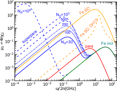
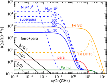
The susceptibility of ferromagnetic single-domain (SD) particles from DL99 and the average susceptibility () from DH13 with are shown in Figure 1 (see orange lines). For frequencies GHz relevant for grain alignment under interest in this paper, two models are only different by a numeric factor, and become identical when is increased by a factor of .
2.4. Big grains with magnetic inclusions
The incorporation of magnetic particles with iron atoms per particle into a big nonmagnetic grain is expected to greatly enhance the grain magnetic susceptibility.222For Fe with mass density , with . Although the possibility of having magnetic inclusions in big carbonaceous grains may not be ruled out,333Yet, if it happens, big carbon grains with inclusions would be aligned with magnetic fields, which is currently not observed. in this paper, we only consider the case of magnetic inclusions in big silicate grains.
2.4.1 Single-domain ferromagnetic inclusions
Let us assume that single-domain ferromagnetic inclusions are randomly distributed in a big grain, and that each inclusion is spontaneously magnetized along its easy-axis. In an applied field , 2/3 of inclusions have their spontaneous magnetizations perpendicular to , which contribute to the susceptibility. And 1/3 of inclusions have parallel to , which do not contribute to the susceptibility (DL99). The zero-frequency effective susceptibility per unit volume of the composite grain is given by
| (9) |
and is then evaluated by Equation (6) where is substituted with (see DL99).
2.4.2 Superparamagnetic inclusions
When ferromagnetic inclusions are sufficiently small so that thermal energy can exceed the energy barrier to reorient the inclusion magnetic moments, then thermal fluctuations within the grain can induce considerable fluctuations of the inclusion magnetic moments. In thermal equilibrium, the average magnetic moment of the ensemble of magnetic inclusions can be described by the Langevin function with argument , where is the total magnetic moment of the cluster, and is the applied magnetic field (Jones & Spitzer 1967; henceforth JS67). The composite grain exhibits superparamagnetic behavior, which has the magnetic susceptibility given by
| (10) |
where is the number of iron clusters per unit volume (JS67).
Plugging and with the total number of clusters into Equation (10), one obtains:
| (11) |
where is the volume filling factor, and .
Superparamagnetic inclusions undergo thermally activated remagnetization at rate
| (12) |
where and (see Morrish 2001). The frequency dependence susceptibility is then evaluated by Equation (6) where and .
The total magnetic susceptibility of superparamagnetic grains now becomes (DL99)
| (13) |
where is dominant for low frequencies of GHz, and dominates for GHz (see Figure 1, left panel).
2.4.3 Effect of ferromagnetic inclusions on paramagnetic atoms
Ferromagnetic inclusions in a big silicate grain generate static magnetic fields acting on nearby paramagnetic (iron) atoms, which is found to significantly increase the magnetic susceptibility of the composite system through spin-lattice relaxation (Duley 1978). The total magnetic susceptibility is equal to
| (14) |
where and are the spin-lattice and spin-spin relaxation times, and the susceptibility of the ordinary paramagnetic material is
| (15) |
where with the atomic density is the fraction of paramagnetic (Fe) atoms, and .
The factor reads
| (16) |
where is the heat volume capacity at constant magnetization, Oe for various paramagnetic materials, and is the rms value of the magnetic field in a given direction outside the ferromagnetic inclusions (see Draine 1996).
Let be the fraction of the total atoms present in single-domain ferromagnetic inclusions. Then,
| (17) |
With the typical value of , the ferromagnetic-paramagnetic interaction can raise by two orders of magnitude above the susceptibility of the ordinary paramagnetic material (see Figure 1).
Figure 1 also shows the frequency dependence of (left panel), and (right panel) for a variety of magnetic materials considered in this paper, including single-domain Fe nanoparticles (Fe SD), ferromagnetic and superparamagnetic inclusions with different , and ferromagnetic-paramagnetic interactions. Results for the ordinary paramagnetic material () are also shown for comparison. Ferromagnetic susceptibility is the most important for high frequencies of GHz, which result in magnetic dipole emission (DL99; DH13).
3. Rotational damping and excitation for magnetic particles
3.1. Electric dipole and magnetic dipole moments
Unlike PAHs, ferromagnetic particles do not possess intrinsic electric dipole moment because of the lack of polar bonds. In principle, any particles may have a net electric dipole moment when the charge distribution is asymmetric such that the charge centroid is displaced from the grain center of mass. However, due to high conductivity, magnetic particles cannot maintain such dipole moment because free electrons and holes can easily move in the grain (electron diffusion time much shorter than charging time) (see de Heer & Kresin 2009 for a review).
At low temperatures, a magnetic particle of volume has an intrinsic magnetic moment due to spontaneous magnetization given by:
| (18) |
where and 1 D statC.cm.
Thus, iron particles of G have largest value of D, slightly lower than the electric dipole moment of PAHs with D at nm (see DL98). Note that rotational emission power by the magnetic dipole varies with grain size as , instead of for the case of the electric dipole, which reveal that larger magnetic grains seem to emit more spinning radiation than the electric grains.
3.2. Damping and Excitation Coefficients
Rotational damping and excitation for dust grains in general arise from collisions between grains and gaseous atoms followed by the evaporation of atoms/molecules from the grain surface, absorption of starlight and IR emission (DL98; HDL10). If the grain posses electric dipole moment, the distant interaction of the grain electric dipole with passing ions results in an additional effect, namely plasma drag. The damping and excitation for these processes are described by the dimensionless damping coefficient and excitation coefficient , respectively (see Appendix B.2).
It is well-known that, for UV-IR photons with GHz, the magnetic properties of dust grains can be ignored in calculations of absorption cross-section due to the dominance of electric dipole cross-section (see DL99; DH13). In this case, grain charging for magnetic grains may be treated by the similar model as silicate grains (see Weingartner & Draine 2001), and collisional damping and excitations of magnetic grains are computed as in DL98. Damping and excitation by IR emission is also computed using the general approach in DL98, and the factor increase in the excitation coefficient is included (see HDL10).
For a magnetic grain, distant interactions with passing ions is also possible through the interaction of spontaneous magnetization with the magnetic field generated by moving ions in the grain’s frame. However, this effect is negligibly small as shown in Appendix B.3.
Moreover, rotational emission by magnetic dipole moment results in the rotational damping. The characteristic damping time due to dipole emission is calculated with Equation (B8) by replacing with , where the magnetic dipole is assumed to be in the plane perpendicular to the grain symmetry axis. We found that the rotational dipole damping is rather inefficient for magnetic nanoparticles.
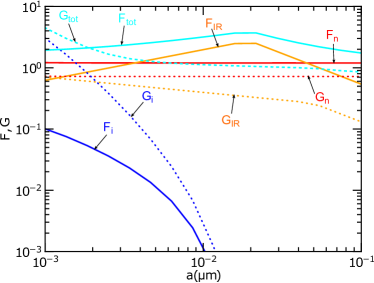
Figure 2 shows the values of and for various processes for ferromagnetic grains in the cold neutral medium (CNM; gas density and temperature ) computed for an oblate spheroidal grain rotating along its symmetry axis. As shown, IR emission is dominant for rotational damping of small grains (), and neutral collisions are dominant for rotational damping/excitation for larger grains. Ion collisions dominate rotational excitation of ultrasmall grains in which the grains are negatively charged due to electron capture.
4. Magnetic Alignment of thermally rotating grains
4.1. Davis-Greenstein Magnetic Relaxation
Davis & Greenstein (1951) (henceforth DG51) suggested that a paramagnetic grain rotating with angular velocity ! in an external magnetic field experiences paramagnetic relaxation, which dissipates the grain rotational energy into heat. This results in the gradual alignment of ! and with the magnetic field at which the rotational energy is minimum.
Let us consider a spinning oblate spheroid with isotropic magnetic susceptibility. This isotropic susceptibility occurs in some materials, including big grains with randomly oriented magnetic inclusions, superparamagnetic grains. The rotating magnetic field component in the grain frame is decomposed into two components along and , such that . The rotational energy dissipation is approximately given by
| (19) |
where .
Ferromagnetic and ferrimagnetic particles exhibit anisotropic susceptibility determined by the spontaneous magnetization . Assuming that the easy axis (i.e., ) is along a long axis 444This situation is idealized because oblate iron particles exhibit equatorial plane of saturation., and the grain is spinning along the short symmetry axis , then, the rotating magnetic field in the grain frame that results in energy dissipation is .555For simplicity, previous studies of ferromagnetic alignment usually assumed prolate spheroids because the spontaneous magnetization is directed along the grain symmetry axis (Henry 1958; Jones & Spitzer 1967). Meanwhile, the Davis-Greenstein alignment is usually treated for oblate spheroids (Lazarian 1997; Roberge & Lazarian 1999, henceforth RL99). Here, we consider oblate spheroid for the sake of consistency. As a result, we have
| (20) | |||||
where .
The characteristic timescale for the magnetic alignment of with is obtained by setting :
| (21) |
where from Equation (B1) has been used.
To describe the effect of grain alignment by magnetic relaxation against the randomization by gas atoms, a dimensionless parameter is usually used:
| (22) |
where is the gaseous damping for the rotation around the grain symmetry axis, , , , and is a geometrical factor (see Appendix B.2).
The grains have for the ordinary paramagnetic material, and for the superparamagnetic and ferromagnetic materials (see Figure 1). In the absence of suprathermal rotation, it follows that paramagnetic grains are likely randomized by gas collisions well before the magnetic relaxation, whereas magnetic relaxation rapidly brings superparamagnetic/ferromagnetic grains to be aligned with the magnetic field. However, the magnetic alignment for the latter materials is still not perfect, as shown in our next section.
4.2. Resonance Magnetic Relaxation
Resonance magnetic relaxation has been shown to be important for the weak alignment of PAHs (Lazarian & Draine 2000; Hoang et al. 2013, 2014, hereafter HLM13, HLM14), and it becomes dominant over the normal paramagnetic relaxation when the grain rotation frequency exceeds the spin-spin relaxation rate . For ferromagnetic particles, it is easy to see that resonance relaxation is unimportant because these particles have , which is still larger than the thermal rotation speed (see Eq. B5) for tiny particles of nm.
4.3. Degrees of Grain Alignment
Let with be the degree of internal alignment of the grain symmetry axis with , and let with be the degree of external alignment of with . Here is the angle between and , and the angle brackets denote the average over the ensemble of grains. The net degree of alignment of with , namely the Rayleigh reduction factor, is defined as .
5. Numerical Method and Results
5.1. Numerical Method
As in previous works (RL99; HLM14), to study the alignment of the grain angular momentum with the ambient magnetic field , we solve the Langevin equations for the evolution of in time in an inertial coordinate system denoted by unit vectors where is chosen to be parallel to . The Langevin equations (LEs) read
| (23) |
where are the random variables drawn from a normal distribution with zero mean and variance , and and are the drifting (damping) and diffusion coefficients defined in the system.
The drifting and diffusion coefficients in a frame of reference fixed to the grain body, and , are related to the damping and excitation coefficients ( and ) as follows:
| (24) | |||||
| (25) | |||||
| (26) |
where and for (or ) are the total damping and excitation coefficients from various processes, and . Finally, and are obtained by using the transformation of coordinate systems for from to (see HLD10; HLM14).
To incorporate magnetic relaxation, we need to add a damping term to and an excitation term to and , respectively. In the dimensionless units of and , Equation (23) becomes
| (27) |
where and
| (28) | |||||
| (29) |
Above, for and for , and
| (30) |
where and are the effective damping times due to dust-gas interactions and electric dipole emission (see Eq. E4 in HDL10).
To numerically solve the Langevin equation (27), earlier works (RL99; HLM14) usually used the first-order integrator, namely Euler-Maruyama algorithm. As shown in Vanden-Eijnden & Ciccotti (2006), the second-order integrator is about one order of magnitude more accurate than the first-order one. For the second order, the angular momentum component at iterative step is evaluated as follows:
| (31) |
where is the timestep, , , , and
| (32) | |||||
| (33) |
with and being independent Gaussian variables with zero mean and unit variance and (see Appendix C for details).
The timestep is chosen by . The angular momentum and the angle between and obtained from the LEs are employed to compute the net degree of alignment as follows:
| (34) |
where can be replaced by with in the case of fast internal relaxation (see e.g, RL99). As usual, the initial grain angular momentum is assumed to have random orientation in the space and magnitude (i.e., ).
For magnetic grains, is determined essentially by two timescales and (or a single parameter ), and the value of can be huge (i.e., ). In this case, a tiny timestep is needed to achieve sufficient statistics, which requires a huge number of time steps (e.g., ) and large computing time. In the following, a fixed integration time is chosen, which ensures that is much larger than the longest dynamical timescale to provide good statistical calculations of the degrees of grain alignment. We adopt the typical CNM phase of the interstellar medium for calculations.
5.2. Big silicate grains with ferromagnetic inclusions
We first quantify the magnetic alignment for thermally rotating big silicate grains incorporated with iron clusters, which give rise to superparamagnetic and ferromagnetic materials. Several values of grain size and a typical dust temperature K are considered. For each value of , we vary from with volume filling factor . A variety of interaction processes is considered, although the dominant interaction for the grains is gas-grain collisions (see Figure 2).
Figure 3 (left panel) shows the obtained values of and as functions of for superparamagnetic grains. The value of rapidly increases with increasing () and slightly varies for (). tends to decrease with increasing () as a result of faster magnetic dissipation. The value of rapidly increases with first and then becomes nearly independent on for (or ), which is referred to as alignment saturation regime. Moreover, the alignment saturation occurs with and for the assumed environment conditions. Bigger grains tend to have higher degree of alignment saturation due to their lower rotational damping (see Figure 2).
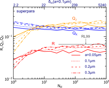
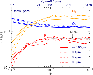
Figure 3 (right panel) shows and as functions of –the fraction of the total atoms in the grains present in iron clusters (see Equation 14) when the effect of ferromagnetism on the paramagnetic grain is accounted for. The value of tends to increase with increasing , whereas tends to decrease with increasing () as seen with superparamagnetic grains. The value of rapidly increase with first up to () and reach alignment saturation with for .
The alignment saturation observed for big grains with ferromagnetic inclusions is resulting from the detailed balance of magnetic dissipation and fluctuations when . In this saturation regime, the alignment becomes independent of the magnetic relaxation and only depends on other processes acting in the parallel direction to . We also found that, due to the additional IR damping included, our saturation levels are slightly lower than the semi-analytical results obtained in RL99 for the same conditions (), as shown by dotted line in Figure 3.
5.3. Free-flying magnetic particles
In the following, we are going to compute the degree of alignment for single-domain ferromagnetic particles with susceptibility given by Equation (6) for (21) for the range of grain size .
5.3.1 Alignment subject to neutral-grain collisions
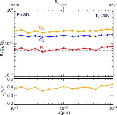
We first consider the case in which grain rotational dynamics is purely induced by neutral-grain collisions and magnetic relaxation that follow detailed balance. The obtained results for K and the DL99 susceptibility form are shown in Figure 4. The degrees of alignment appear to decrease slightly with decreasing the grain size from or increasing from (upper panel). The similar trend is seen for the variation of (lower panel). This alignment saturation is reminiscent of what seen in the case of big grains with ferromagnetic inclusions of .
5.3.2 Alignment in the presence of various interaction processes
Now we take into account all interaction processes, including IR emission and ion collisions that do not follow detailed balance. Three values of and K are considered.
Figure 5 show the results computed with the magnetic susceptibility from DL99. First, the degree of alignment does not exhibit alignment saturation but varies significantly with despite (i.e., being in the saturation regime). When is decreased from , and decrease with decreasing until their minimum around and reverse their trend for smaller . In particular, the degree of alignment varies with in a similar trend as (see the lower part of each panel). Second, higher result in lower degrees of alignment but higher value of due to stronger thermal fluctuations (Lazarian 1994; Lazarian & Roberge 1997) (see lower panels). Moreover, the location of the minimum tends to shift to smaller grain sizes for higher .
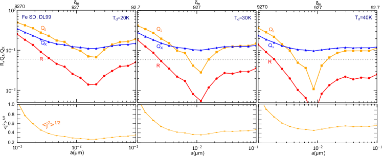
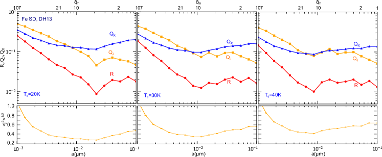
Figure 6 present the degrees of alignment computed with the magnetic susceptibility from DH13 (see Equation 8). The results exhibit remarkable similarity with those obtained with the DL99 susceptibility (see Figure 5), in which the alignment minimum occurs at , and the alignment increases rapidly with decreasing from that position. The obvious difference in alignment occurs for where the magnetic relaxation rate is moderate of (i.e., not yet in the alignment saturation regime) in which the value of increases with increasing .
The disappearance of alignment saturation for ferromagnetic nanoparticles with in the presence of ion-grain collisions and IR emission can be understood as follows. In the case of extreme magnetic dissipation (), the torques perpendicular to are essentially the magnetic torque, while the torques parallel to are determined by a variety of other interaction processes including imbalanced ones. The latter determine how fast the grain is spinning statistically, i.e., the value of that determines the ultimate degree of magnetic alignment. Therefore, when the excitation by ion collisions increases and/or the damping by IR emission decreases (see Figure 2), it results in an increase in and then the degree of alignment of ultrasmall grains of (see Figure 5 and 6). The increase of IR damping results in the decrease of alignment of small particles of .
6. Polarization of magnetic dust emission
The polarization of MDE from free-flying magnetic nanoparticles is calculated as the following:
| (35) |
where and are the radiation intensity with the electric field parallel to and in the plane of the sky (see Appendix A.2 for more details).
In the presence of the imperfect alignment, and are given by
| (36) | |||||
| (37) | |||||
where , , is the size distribution of magnetic particles, is the Planck function, and is the angle between the magnetic field and the plane of the sky (see Lee & Draine 1985; RL99).
6.1. Single-size magnetic nanoparticles
First, we assume that magnetic particles have the size distribution (i.e., grains of single size ). The relative number density of magnetic particles per H is , where is the grain volume per H of material Y. Following DL99, , where and are the fraction of total Fe incorporated and the fraction of Fe mass of material , respectively. Here is the grain volume per H for a typical material that accommodates the entire budgets of Mg, Si, and Fe (see DL99).
For metallic iron with and , it follows that . Similarly, we obtain for , and for with and , respectively.
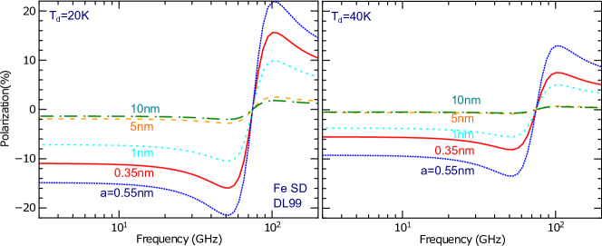
Figure 7 shows the polarization spectra of MDE computed for an oblate spheroid of single sizes using the DL99 susceptibility. First, the polarization reverses its sign from negative to positive at GHz where electric dipole emission becomes dominant. Moreover, MDE from smaller grains has higher degree of polarization, as expected from the computed degrees of alignment (see Figure 3). In particular, if iron particles are larger than nm, then, the polarization of its MDE is below .
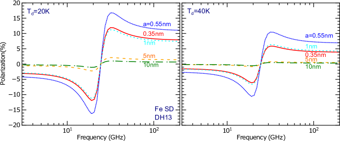
Figure 8 shows the polarization spectra obtained using the susceptibility form from DH13. The polarization is essentially lower than shown in Figure 9 due to its lower degree of alignment. In particular, due to the lower susceptibility, the reverse in polarization sign occurs at lower frequency than in the case of the DL99 susceptibility (i.e. electric dipole emission dominate magnetic emission at lower frequency).
6.2. Size distribution of magnetic particles
Now let us assume that all Fe abundance is present in the form of small clusters of radius from . At low temperatures, even very small iron clusters are ferromagnetic (i.e., having spontaneous magnetization), so we can take nm or (Billas et al., 1994). The upper size is chosen as the critical size of single-domain, i.e., nm. Because there is no clue about any specific size distributions, we assume a typical power law (Mathis et al. 1977), where is a normalization constant determined by the grain volume per H:
| (38) |
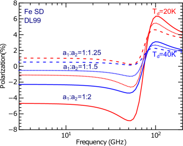
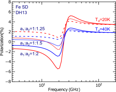
The polarization spectra are shown in Figure 9 two cases of the DL99 (left panel) and DH13 (right panel) susceptibility. We can see that the polarization of integrated MDE is rather low (e.g, less than for K), which is substantially lower than the MDE polarization from nanoparticles of single radius of nm. This feature is due to the fact that the intensity of MDE depends on the grain volume for which the largest particles dominate the MDE. However, those larger particles are found to have the lower degree of alignment due to stronger IR damping (see Figure 5). The polarization using DH13 susceptibility is slightly lower due to lower susceptibility.
7. Spinning dust emission by free-flying magnetic particles
Spinning magnetic particles with permanent magnetic moments emit microwave emission by the same mechanism as spinning electric dipole emission (Erickson 1957). The spinning emissivity can be computed by the same model of HDL10, but the electric dipole moment is replaced by the magnetic dipole . We consider oblate spheroidal grains with axial ratio for a typical model.
The polarized emissivity and unpolarized emissivity of spinning dust emission are calculated as follows:
| (39) | |||||
| (40) |
where is the spinning dust emissivity at frequency from a grain of size , and nm is assumed. As in the previous section, we consider two cases of single-size particles and those following the MRN distribution. The polarization spectrum of spinning dust emission is .
Figure 10 shows the unpolarized emissivity and polarized emissivity for the single-size case with and 2 nm. Smallest Fe particles emit considerable spinning emissivity, but it is still one order of magnitude lower than that from spinning PAHs (see, e.g., Figure 13). We also computed the spinning emission from ferrimagnetic particles (Fe2O3 and Fe3O4) and found that their emission is much lower than spinning metallic iron, which is expected due to their much smaller . Notably, the polarization degree of spinning emission from iron particles is rather high, up to for K. This is a direct result of the efficient external alignment of tiny iron particles as shown in Figure 4.
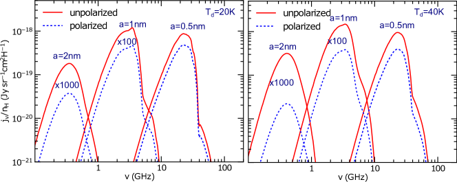
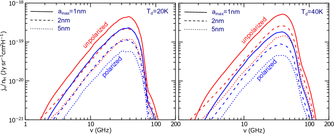
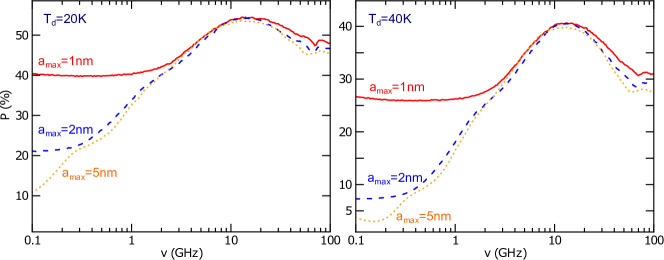
Figure 11 shows the emissivity for the case of the MRN distribution with and 5 nm. The spinning emission is strongest when all iron atoms are concentrated in the range nm. The peak emissivity is insensitive to , which is expected from the fact spinning emission is dominated by smallest grains having the fastest rotation and the contribution from larger grains is negligible (see Figure 10). The polarization of spinning emission from iron particles can reach for the magnetic field in the plane of the sky (see Figure 12), which originate directly from high degree of alignment (i.e., ) of ultrasmall iron particles (see Figure 5).
8. Discussion
8.1. Magnetic dipole emission from magnetic nanoparticles
Magnetic dipole emission (MDE) was first suggested in DL99 as a potential source of AME for frequencies of GHz. In this original model, the magnetic response of the ferromagnetic material to an applied oscillating magnetic field is treated using the Drude model with scalar susceptibility. Recently, DH13 revisited the treatment of magnetic response by using the Gilbert equation with tensor susceptibility, where the magnetization damping is characterized by a dimensionless Gilbert parameter . With a new form of magnetic susceptibility, DH13 found that MDE is important for frequencies of GHz.
Thus, more experimental and theoretical studies are undoubtedly necessary to better understand the susceptibility of magnetic material at high frequencies and to differentiate the emission spectrum of MDE predicted by the two models. The pressing issue now is to have quantitative, realistic predictions for the polarization of MDE for reliable detection of CMB B-mode signal. For this purpose, we have used the magnetic susceptibility from both DL99 and DH13 to compute the degree of alignment for ferromagnetic nanoparticles and obtained the MDE polarization spectra for both models.
8.2. Degree of alignment of thermally rotating magnetic grains
The first study on magnetic alignment of thermally rotating grains that takes into account the effect of imperfect Barnett relaxation (Purcell 1979; Lazarian & Roberge 1997) was performed in Lazarian (1997) using the analytical method. RL99 used the numerical method based on the Langevin equation to compute the degree of alignment for both paramagnetic and superparamagnetic grains of different values of axial ratio , and . The RL99’s study only considered the alignment of big grains subject to neutral-grain collisions and superparamagnetic relaxation of .
The present work first improved the numerical method in RL99 by implementing a second-order integrator for solving the Langevin equations, and extended calculations for a wider range of . We find that thermally rotating superparamagnetic grains are weakly aligned and achieve alignment saturation of for . We also have quantified the effect of ferromagnetic and paramagnetic interactions on the alignment of big silicate grains for a wide range of the fraction of iron in clusters . Same as thermally rotating superparamagnetic grains, the degree of alignment is low and becomes saturated for or . One consequence of the alignment saturation for the grains with superparamagnetic/ferromagnetic inclusions is that the dust polarization becomes independent on the magnetic field strength (cf. HLM14) and depends mostly on the magnetic field direction.
Second, we have computed the degrees of alignment of single-domain ferromagnetic nanoparticles, accounting for various rotational damping and excitations by neutral-grain collisions, ion collisions, and IR emission, using the susceptibility form from both DL99 and DH13. It is noted that the ultrasmall iron particles can have very large value of , which requires significant computing time to obtain good statistics. Interestingly, we found that the alignment saturation expected for is destroyed in the presence of imbalanced interaction processes. Specifically, we identify that rotational excitation from ion collisions, which becomes more efficient for tiny grains of negatively charge, can enhance the alignment of very small iron grains (), whereas strong IR damping can significantly reduce the alignment of particles. This result indicates that even subtle excitation/damping by imbalanced processes (e.g., ion collision and IR emission) can have a great impact on the alignment of grains in the alignment saturation regime . Notably, we found no clear difference in the degree of alignment of very small iron grains between the susceptibility form from DH13 and DL99. This is due to the fact that both models yield (i.e., saturation regime) such that the alignment efficiency becomes independent of the magnetic relaxation rate.
Lastly, the low degrees of alignment for thermally rotating, superparamagnetic grains in realistic environmental conditions (i.e., not much larger than ) indicate that suprathermal rotation is required for producing efficient alignment, as required by observations (see latest reviews in Andersson et al. 2015; Lazarian et al. 2015). If magnetic nanoparticles are incorporated into big grains, then such grains have greatly enhanced magnetic susceptibility, either through superparamagnetic clusters or the ferro-paramagnetic interaction. As a result, the joint action of radiative torques and the enhanced magnetic dissipation would likely lead to efficient alignment (Lazarian & Hoang, 2008). Detailed study will be presented in our future paper.
8.3. Polarization of magnetic dipole emission: free-fliers vs. magnetic inclusions
Magnetic nanoparticles, whether being free-fliers or inclusions, produce slightly different MDE spectra (DL99; DH13), while the polarization of MDE from these two forms is usually believed to be distinct. For instance, assuming its perfect alignment with the interstellar magnetic field, DL99 predicted that free-flying iron spheroids produce high polarization level ( for GHz), whereas randomly oriented ferromagnetic inclusions would produce low polarization level. In DH13, the MDE polarization is also expected to be large (i.e., can reach ) for free-flying magnetic nanoparticles and a lower level for big grains with magnetic inclusions. Yet, we have found that the polarization level of MDE from free-flying iron nanoparticles is rather small for both the DL99 and DH13 susceptibility forms.
Indeed, MDE by free-flying magnetic particles increases with the particle volume, so does its polarization level. For the size range of nm where single-domain iron clusters are expected to exist in the ISM conditions, the largest particles dominate MDE and its polarization level. Meanwhile, we found that these large particles tend to have much lower degree of alignment than the smallest ones, with the minimal alignment at nm due to strong IR damping. Therefore, unless magnetic particles are ultrasmall of nm for which the MDE polarization can reach 20 () for K (40K), the polarization of MDE is predicted to be below at K (see Figure 7 and 9). The polarization spectrum for the DH13 susceptibility reverses its sign at GHz, lower than GHz for the DL99 model, which is directly resulting from its lower magnetic susceptibility.
It is noted that the polarization of MDE from magnetic inclusions depends on the alignment of big silicate grains, which tends to vary with the local radiation intensity according to the radiative alignment theory ((Lazarian et al., 2015)). On the other hand, the MDE polarization from free-flying particles does not depend on the radiation field. Thus, it may be possible to search for the form of magnetic particles by studying the MDE polarization from the diffuse medium and dense clouds. If the variation of the MDE polarization is observed toward the denser regions, then, the MDE may be produced by magnetic inclusions instead of free-flying particles.
8.4. Polarization of spinning dust emission from magnetic particles
8.4.1 Free-flying magnetic nanoparticles
We have investigated spinning emission by spontaneous magnetization of magnetic particles and found that the largest emissivity is still one order of magnitude lower than spinning PAHs when all iron budget is present in single-size nanoparticles with . One distinct feature of spinning emission from ferromagnetic particles is of its high degree of polarization, which can reach (see Figure 12). Such a difference arises from the fact ferromagnetic nanoparticles have and do not suffer the suppression of magnetic relaxation due to fast rotation (i.e., still lower than the spin-relaxation rate ). In addition, the rotational damping by spinning radiation that removes the grain angular momentum is very weak for magnetic particles due to its small dipole moment.
8.4.2 Big grains with magnetic inclusions
Big silicate grains are likely spinning suprathermally due to radiative torques (RATs; Draine & Weingartner 1996; Lazarian & Hoang 2007) and pinwheel torques (e.g., due to H2 formation; Purcell 1979; Hoang & Lazarian 2009). The existence of ferromagnetic inclusions in such suprathermally rotating big grains would induce rotational radiation.
Let us assume that iron clusters are randomly oriented in a big nonmagnetic grain. The net magnetic moment of the grain is estimated to be
| (41) |
where is the magnetic moment of each cluster.
The emission power by the grain rotating at is equal to
| (42) | |||||
For the MRN distribution, we can estimate the total emission intensity per H atom as follows:
| (43) | |||||
where , and .
If RATs are the main spin-up processes, we have (Hoang & Lazarian, 2009) for where is the ratio of the radiation energy relative to the average radiation density in the solar neighborhood. Thus, one has , or where . The emissivity is clearly negligible compared to that from spinning PAHs in the ISM with . In the star forming regions with strong radiation (i.e., ), the spinning emission can be in the radio with GHz, but it appears that the intensity of spinning radiation is unimportant.
Our above estimates are for the rotation around the grain symmetry axis. In fact, due to incomplete internal relaxation (Lazarian 1994; Lazarian & Roberge 1997) grains may not rotate around the axis of maximal inertia, resulting in wobbling motion. As a result, the emission by an isolated, spinning triaxial grain occurs at many modes, which allows more energy to be extracted from the rotational energy (HDL10; Hoang et al. 2011, hereafter HLD11). As a result, the total emissivity can be increased by a factor of 2, and peak frequency is increased by a factor 1.5 (HDL10). Moreover, the effect of transient spin-up by ion collisions and turbulence can also enhance the spinning dust emission. It seems that even including all these effects, spinning emission from big grains of magnetic inclusions is still negligible.
8.5. Polarization of spinning dust emission from PAHs
During the last few years, we have witnessed significant progress in improving the dynamical models of spinning dust emission (HDL10; HLD11; Silsbee et al. 2011). Meanwhile, the polarization of spinning dust emission, which is essential for reliable measurements of CMB B-mode signal, is still uncertain. Nevertheless, its polarization is certainly determined by the alignment of PAHs, which is believed due to resonance paramagnetic relaxation (Lazarian & Draine 2000; HLM14). Using inversion technique combined with theoretical calculations, Hoang et al. (2013) found a level of polarization for the line of sight toward a star (HD 197770) with the 2175 polarization bump.
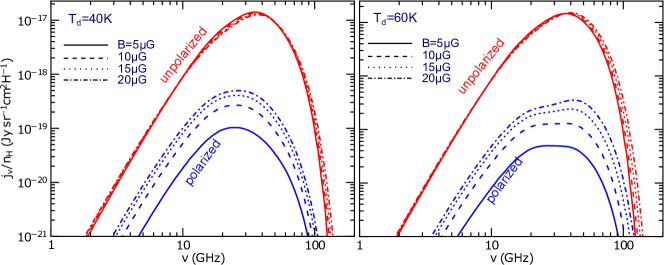
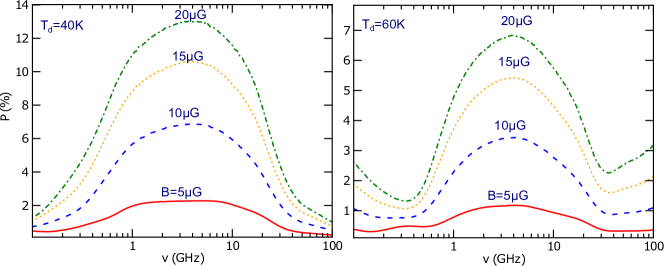
In Figure 14, we present the theoretical polarization spectra of spinning emission from PAHs in the CNM, computed for the different magnetic field strength with direction in the plane of the sky () at and K. The value of is assumed. For the typical value of G, the polarization is less than for GHz. Colder spinning PAHs tend to generate stronger polarized emission due to weaker internal thermal fluctuations. Particularly, the polarization by spinning PAHs is lower than that by spinning Fe nanoparticles because the latter has much higher and does not suffer magnetic suppression due to the rapid rotation because the spin-spin relaxation rate still exceeds the rotation rate.
The theoretical predictions for the polarization of spinning PAH emission appear to be consistent with the available observational data. For instance, several observational studies (Battistelli et al. 2006; Mason et al. 2009; Dickinson et al. 2011; Battistelli et al. 2015) have found the upper limits for the AME polarization to be between and . An upper limit of is also reported in various studies (see López-Caraballo et al. 2011; Rubiño-Martín et al. 2012). Latest results by Planck (Collaboration et al. 2015) show the AME polarization to be .
8.6. On Mysterious Origin of AME
Numerous observations have revealed that AME is most likely produced by rapidly spinning tiny dust grains (mostly PAHs) (see e.g., Planck Collaboration et al. 2011; Collaboration et al. 2015). Especially, the low polarization level predicted for spinning dust emission from PAHs is in good agreement with the observational data (see the previous section).
Hensley et al. (2015) (hereafter HDM) found a weak correlation of AME with PAH abundance using all-sky AME map, which reveals that AME might not originate from spinning PAHs. The paper suggests reconsideration of other origins for AME. If the spinning PAH theory as it is formulated in DL98 and improved in HDL10, indeed, has problems explaining the observational data as claimed in HDM, we suggest several alternatives: (a) Physics of PAH is more complex than it was assumed by DL98, e.g. the dipole moment changes with the environment in a way to offset the predicted correlations. (b) The emission is still from spinning dust, but the dust of not PAH nature. Iron and silicate nanoparticles are the primary candidate. (c) The role of magnetic dust emission should be reconsidered. (d) The AME does not originate from dust, but has a completely different nature.
The physics that can change PAHs and then its spinning emission to satisfy the analysis of HDM is unclear. However, there has not been enough studies of interstellar PAHs to dismiss this opportunity. This leaves the case (a) somewhat in limbo.
Regarding the issue (b), in the present paper, we have quantified spinning emission from iron nanoparticles and found that its rotational emission is maximum within the AME frequency range but has low emissivity of . Yet the emission from spinning iron particles is highly polarized. The case of silicate nanoparticles looks like a possibility. But our initial estimates show that spinning emissivity from tiny silicate grains of SiO structure having large dipole moment (D per structure ) is also small if they follow the size distribution of Draine & Li (2007). Thus, it requires a substantial population of silicate nanoparticles to produce higher spinning emissivity, and the processes of their formation stay unclear. However, interstellar dust has always presented us with surprises. It is clear that more work in formulating spinning dust theory of silicate nanoparticles in analogy with the existing spinning PAH theory is necessary as well as the search for the observational features that can test this hypothesis. Unlike the population of PAH, which has been proven to exist, the population of silicate nanoparticles is a hypothesis, which requires testing, e.g., through identifying particular spectral features related to the emission of these particles. This makes case (b) an interesting hypothesis that requires intensive testing.
Our present work is intended to address the issue of the polarization of MDE arising from strongly magnetic particles, in particular, free-flying nanoparticles. The discussions of MDE polarization were given for two different forms of magnetic susceptibilities given in DL99 and DH13, respectively. Although DH13 provide arguments in favor of the susceptibility that it accepted, the fit of the magnetic response to the high frequency experimental data that DH13 present is poor. It is therefore necessary to provide laboratory studies of candidate materials for the required range of frequencies, which includes the AME frequency range. We believe that this presents an important avenue for future studies related to the case (c). Moreover, the MDE by free-flying magnetic particles was frequently ruled out as a source of AME appealing to its high expected polarization level (López-Caraballo et al. 2011; Collaboration et al. 2015; Génova-Santos et al. 2015). Our obtained results however indicate that the polarization of MDE from free-fliers is rather low, and its maximum level depends weakly on the specific form of magnetic susceptibility. Therefore, MDE from free-flying nanoparticles cannot be ruled out as a source of AME by means of polarization constraints and may be more important for AME than usually thought.
Finally, the existing problems call for revisiting ideas of non-dust sources of AME. So far, such attempts have been futile, but they were based on the incomplete knowledge of the foreground properties. For instance, the synchrotron properties may be changed by the peculiar structure of magnetic field and so the synchrotron emission spectrum. Studies of propagation as well as observational studies of the magnetic field, e.g. with new techniques suggested in Lazarian & Pogosyan (2015), may clarify the situation. We feel, however, that the case (d) is most speculative at the moment.
9. Summary
In this paper, our principal results are summarized as follows:
-
1
The degrees of alignment of thermally rotating silicate grains incorporated with iron nanoparticles are computed for a wide range of iron atoms per cluster and the fraction of atoms in clusters (characterized by . We find that the degrees of alignment first increase with and reach alignment saturation at and for for the typical conditions of the ISM. The alignment saturation indicates that, without suprathermal rotation, silicate grains with magnetic inclusions are only weakly aligned.
-
2
We have computed the degree of alignment of ferromagnetic single-domain particles, accounting for a variety of rotational damping and excitation processes. We find that the rotational damping by IR emission significantly decreases the alignment of small particles, whereas the excitation by ion collisions enhances the alignment of ultrasmall grains from the saturation level. We have also computed the alignment of Fe nanoparticles using the new susceptibility derived by DH13 and found that the degrees of alignment become independent of the specific susceptibility form when the magnetic damping is much faster than the rotational damping (i.e., ).
-
3
Using the computed degrees of alignment, we have predicted the polarization of MDE by free-flying iron nanoparticles. In contrast to common belief of its high polarization, we found that the polarization of MDE from free-fliers with radii of several nanometers is below for the typical K. Thus, the MDE by free-flying iron nanoparticles may not be ruled out as a source of AME by appealing to the upper limits of the AME polarization.
-
4
Spinning dust emission from iron nanoparticles with permanent magnetic moments is found to be inefficient, but its polarization level is rather high, up to . The largest emissivity by iron particles is one order of magnitude lower than the emission by spinning PAHs, assuming that all Fe abundance is present in single-size nanoparticles.
-
5
We have calculated the polarization of spinning dust emission from PAHs for the different magnetic field strengths. The polarization is below for the typical physical parameters (e.g., G and K), which suggests that spinning dust emission by PAHs can be distinguished from spinning magnetic nanoparticles by means of the polarization signature.
Appendix A A. Polarization of magnetic dust emission by free-fliers in the presence of imperfect alignment
A.1. A1. Coordinate system
Let be the grain principal axes where is the axis of maximum moment of inertia. Let are unit vectors in which is parallel to . The observer coordinate system is defined by where is pointed toward the observer. Let be unit vectors defined by the magnetic field in which , and the magnetic field is assumed to be in the plane and makes an angle with . With the angles defined in the figures, we have the following:
| (A1) | |||
| (A2) | |||
| (A3) |
From -frame to -frame, we get
| (A4) | |||
| (A5) | |||
| (A6) |
Finally,
| (A7) |
A.2. A2. Polarization of Magnetic Dipole Emission
The polarization of dipole emission from an ensemble of grains is defined as
| (A8) |
where and are the radiation intensity with the electric field parallel to and in the plane of the sky.
For a single grain, Equation (A8) can be rewritten as
| (A9) |
where , and are total absorbtion cross-section due to dielectric susceptibility and magnetic permeability, which arises from the interaction of the component with electric dipoles and with magnetic moments. The former is dominant for high frequencies (UV, optical and IR wavelengths) while the latter is important for low frequencies (cm and submm).
For an ellipsoidal grain of semiaxes with geometrical factors , the electric cross section for the incident electric field parallel to the semi-axis , and magnetic absorption cross-section for the magnetic field parallel to axis perpendicular to are
| (A10) |
where and are dielectric polarizability and isotropic magnetic permeability (see Bohren & Huffman 1983). So, the cross-section for (or ) along the short axis (larger ) is smaller than the cross-section for along the long axis.
For a simple situation in which the rotation is along the short axis , and both axes are directed along the magnetic field in the sky plane , DL99 got the polarization with
| (A11) | |||
| (A12) |
where is the same as axis, and is the same as axis in DL99. Note that is defined such that incident electric field is along , which directly means is directed along since the wave plane is with propagation direction . Similarly is with and .
When the imperfect alignment of grains with the magnetic field is considered, the polarization (Eq. A9) for oblate grains becomes (see Lee & Draine 1985; RL99)
| (A13) |
where , and , including both electric dipole and magnetic dipole extinction. In this equation,
| (A14) | |||
| (A15) |
for .
The dielectric function for ferromagnetic particles is taken to be
| (A16) |
where and .
Appendix B B.Rotational Damping and Excitation Coefficients for Magnetic Particles
B.1. B1.Grain geometry
We consider oblate spheroidal grains with moments of inertia along the grain principal axes denoted by , and . Let and . They take the following forms:
| (B1) |
where and are the lengths of the semiminor and semimajor axes of the oblate spheroid with axial ratio , and is the grain material density.
The grain size is defined as the radius of an equivalent sphere of the same volume, which is given by
| (B2) |
B.2. B2. Rotational damping and excitation coefficients
We follow the definitions of rotational damping and excitation coefficients from Draine & Lazarian (1998). The dimensionless damping coefficient for the process, , is defined as the ratio of the damping rate induced by that process to that induced by the collisions of gas species, , assuming that the gas consists of purely atomic hydrogen:
| (B3) |
and the excitation coefficient is defined as
| (B4) |
where =n, i, p and IR denote the grain collisions with neutrals and ions, plasma-grain interactions, and the IR emission, is the rate of increase of kinetic energy for rotation along the axis that has moment of inertia due to the excitation process . For an uncharged grain in a gas of purely atomic hydrogen, and .
The thermal angular velocity of a grain around its symmetry axis (of rotational energy ) is
| (B5) |
where .
To calculate the damping and excitation coefficients for wobbling grains, we follow the same approach as in HDL10, where the parallel components and , and perpendicular components and with respect to are computed using the general definitions (Equations B3 and B4). The only modification is the moments of inertia and and and for an oblate spheroid instead of those for disk-like grains in HDL10.
For example, the characteristic damping times of an oblate spheroidal grain for rotation along the directions parallel and perpendicular to the grain symmetry axis are respectively given by (Lazarian 1997)
| (B6) |
where with the grain symmetry axis, and and being the axes perpendicular to the symmetry axis. In the above equation, is the gas density, is the hydrogen mass, is the thermal speed of hydrogen, and the and are geometrical factors (Roberge et al. 1993).
Likewise, the characteristic damping times due to the electric dipole emission from HDL10 can be rewritten as
| (B8) |
where and are the components of the electric dipole moment ¯ parallel and perpendicular to the grain symmetry axis. Here we assume an isotropic distribution of ¯, which corresponds to where is given by Equation (11) in DL98.
B.3. B3. Passing ion-permanent magnetic dipole interactions
Let consider an ion of charge passing a magnetic grain in direction with velocity . The magnetic field produced by the moving charge at the grain position is
| (B12) |
where is the distance from the moving charge to the grain position.
It is easy to see that the magnetic torque is zero when the magnetic moment of the magnetic particle is directed along the axis, and is nonzero when lies in the plane . Let’s assume that is directed along for simplicity. The torque acting on the dipole is then equal to
| (B13) |
For the impact approximation, the ion is assumed to be moving along a straight trajectory (e.g., axis) at constant . The angular momentum impulse induced by the entire ion trajectory is given by
| (B14) |
Therefore, the increase of rotational energy per second is
| (B15) |
where is the rate of incident ions.
Adopting a Maxwellian velocity distribution for ions, we obtain
| (B16) |
where is the mean ion velocity.
As usual, the excitation coefficient is defined as
| (B17) |
Using c.g.s, and plugging numerical parameters into the above equation, it yields . This indicates that the excitation by passing ions is negligible.
Appendix C C. Second-order integrator for Langevin Equation
C.1. C1. Integrator algorithms
Earlier works on numerical calculations of magnetic alignment used the first-order integrator (Euler-Maruyama algorithm) to solve the Langevin equation. In order to account for high accuracy of alignment degree relevant for polarization, we implement second-order integrator. As shown in Vanden-Eijnden & Ciccotti (2006), the accuracy of the second-order integrator is more than one order of magnitude of the first-order.
By setting and omitting the primes in and , Equation (27) can be rewritten as
| (C1) |
where , in our case. The momentum component at is obtained by integrating the above equation from to :
| (C2) |
where the index has been omitted.
Note that , where denotes the equality in distribution, and is a Gaussian random variable with mean zero and unit variance. In the first-order approximation, Equation (C1) yields the solution at iterative step as follows:
| (C3) |
which is well-known Euler-Maruyama algorithm.
To achieve higher accuracy, following Vanden-Eijnden & Ciccotti (2006), we write in Equation (C2) as the follow:
| (C4) |
where .
Using , we get and . Thus, the above equation becomes
| (C6) |
Using the fact that , we have , and
| (C7) | |||
| (C8) |
where and are independent Gaussian variables with zero mean and unit variance, and
Let and . Plugging Equation (C7) and (C8) into (C2) we obtain the following to the second order:
| (C9) |
where
| (C10) | |||||
| (C11) |
The advantage of second-order integrator is that it allows us to achieve the comparable accuracy as the first-order, but with larger timestep , which can save significant computing time.
References
- Ade et al. (2015) Ade, P. A. R., Aghanim, N., Ahmed, Z., & et al. (BICEP2/Keck and Planck Collaborations). 2015, Physical Review Letters, 114, 101301
- Andersson et al. (2015) Andersson, B.-G., Lazarian, A., & Vaillancourt, J. E. 2015, Annual Review of Astronomy and Astrophysics, 53, 501
- Battistelli et al. (2006) Battistelli, E. S., Rebolo, R., Rubiño-Martín, J. A., et al. 2006, ApJ, 645, L141
- Battistelli et al. (2015) Battistelli, E. S., Carretti, E., Cruciani, A., et al. 2015, ApJ, 801, 111
- Bennett et al. (2003) Bennett, C. L., Hill, R. S., Hinshaw, G., et al. 2003, ApJS, 148, 97
- Billas et al. (1994) Billas, I. M. L., Chatelain, A., & de Heer, W. A. 1994, Science, 265, 1682
- Bohren & Huffman (1983) Bohren, C. F., & Huffman, D. R. 1983, Absorption and scattering of light by small particles (New York: Wiley)
- Bouchet et al. (1999) Bouchet, F. R., Prunet, S., & Sethi, S. K. 1999, MNRAS, 302, 663
- Carvell et al. (2010) Carvell, J., Ayieta, E., Gavrin, A., et al. 2010, Journal of Applied Physics, 107, 103913
- Collaboration et al. (2015) Collaboration, P., Ade, P. A. R., Aghanim, N., & Alves, M. I. R. e. a. 2015, arXiv:1506.06660, 6660
- Davis & Greenstein (1951) Davis, L. J., & Greenstein, J. L. 1951, ApJ, 114, 206
- de Heer & Kresin (2009) de Heer, W. A., & Kresin, V. V. 2009, arXiv.org
- Dickinson et al. (2011) Dickinson, C., Peel, M., & Vidal, M. 2011, MNRAS, 418, L35
- Draine (1996) Draine, B. T. 1996, in Astronomical Society of the Pacific Conference Series, Vol. 97, Polarimetry of the Interstellar Medium, ed. W. G. Roberge & D. C. B. Whittet, 16
- Draine & Hensley (2013) Draine, B. T., & Hensley, B. 2013, ApJ, 765, 159
- Draine & Lazarian (1998) Draine, B. T., & Lazarian, A. 1998, ApJ, 508, 157
- Draine & Lazarian (1999) Draine, B. T., & Lazarian, A. 1999, ApJ, 512, 740
- Draine & Li (2007) Draine, B. T., & Li, A. 2007, ApJ, 657, 810
- Draine & Weingartner (1996) Draine, B. T., & Weingartner, J. C. 1996, ApJ, 470, 551
- Duley (1978) Duley, W. W. 1978, ApJ, 219, L129
- Efstathiou (2003) Efstathiou, G. 2003, MNRAS, 346, L26
- Erickson (1957) Erickson, W. C. 1957, ApJ, 126, 480
- Génova-Santos et al. (2015) Génova-Santos, R., Martín, J. A. R., Rebolo, R., & et al. 2015, MNRAS, 452, 4169
- Gilbert (2004) Gilbert, T. L. 2004, IEEE Transactions on Magnetics, 40, 3443
- Henry (1958) Henry, J. 1958, ApJ, 128, 497
- Hensley et al. (2015) Hensley, B. S., Draine, B. T., & Meisner, A. M. 2015, arXiv.org
- Hoang & Lazarian (2009) Hoang, T., & Lazarian, A. 2009, ApJ, 695, 1457
- Hoang et al. (2011) Hoang, T., Lazarian, A., & Draine, B. T. 2011, ApJ, 741, 87
- Hoang et al. (2013) Hoang, T., Lazarian, A., & Martin, P. G. 2013, ApJ, 779, 152
- Hoang et al. (2014) Hoang, T., Lazarian, A., & Martin, P. G. 2014, ApJ, 790, 6
- Jones & Spitzer (1967) Jones, R. V., & Spitzer, L. 1967, ApJ, 147, 943
- Kogut et al. (1996) Kogut, A., Banday, A. J., Bennett, C. L., et al. 1996, ApJL, 464, L5
- Lazarian (1994) Lazarian, A. 1994, MNRAS, 268, 713
- Lazarian (1997) Lazarian, A. 1997, MNRAS, 288, 609
- Lazarian et al. (2015) Lazarian, A., Andersson, B.-G., & Hoang, T. 2015, in Polarimetry of stars and planetary systems, ed. L. Kolokolova, J. Hough, & A.-C. Levasseur-Regourd ((New York:Cambridge University Press))
- Lazarian & Draine (2000) Lazarian, A., & Draine, B. T. 2000, ApJ, 536, L15
- Lazarian & Hoang (2007) Lazarian, A., & Hoang, T. 2007, MNRAS, 378, 910
- Lazarian & Hoang (2008) Lazarian, A., & Hoang, T. 2008, ApJ, 676, L25
- Lazarian & Pogosyan (2015) Lazarian, A., & Pogosyan, D. 2015, arXiv.org, 1537
- Lazarian & Roberge (1997) Lazarian, A., & Roberge, W. G. 1997, ApJ, 484, 230
- Lee & Draine (1985) Lee, H. M., & Draine, B. T. 1985, ApJ, 290, 211
- Leger & Puget (1984) Leger, A., & Puget, J.-L. 1984, A&A, 137, L5
- Leitch et al. (1997) Leitch, E. M., Readhead, A. C. S., Pearson, T. J., & Myers, S. T. 1997, ApJL, 486, L23
- López-Caraballo et al. (2011) López-Caraballo, C. H., Rubiño-Martín, J. A., Rebolo, R., & Génova-Santos, R. 2011, ApJ, 729, 25
- Mason et al. (2009) Mason, B. S., Robishaw, T., Heiles, C., Finkbeiner, D., & Dickinson, C. 2009, ApJ, 697, 1187
- Mathis et al. (1977) Mathis, J. S., Rumpl, W., & Nordsieck, K. H. 1977, ApJ, 217, 425
- Morrish (2001) Morrish, A. H. 2001, The Physical Principles of Magnetism (Wiley-IEEE Press)
- Planck Collaboration et al. (2011) Planck Collaboration, Ade, P. A. R., & Alves, M. I. R. e. a. 2011, Astronomy and Astrophysics, 536, A20
- Planck Collaboration et al. (2011) Planck Collaboration, Ade, P. A. R., Aghanim, N., et al. 2011, A&A, 536, A20
- Planck Collaboration et al. (2013) Planck Collaboration, Ade, P. A. R., Aghanim, N., et al. 2013, arXiv
- Planck Collaboration et al. (2014) Planck Collaboration, Adam, R., Ade, P. A. R., et al. 2014, arXiv:1409.5738, 5738
- Purcell (1979) Purcell, E. M. 1979, ApJ, 231, 404
- Roberge et al. (1993) Roberge, W. G., Degraff, T. A., & Flaherty, J. E. 1993, ApJ, 418, 287
- Roberge & Lazarian (1999) Roberge, W. G., & Lazarian, A. 1999, MNRAS, 305, 615
- Rouan et al. (1992) Rouan, D., Leger, A., Omont, A., & Giard, M. 1992, A&A, 253, 498
- Rubiño-Martín et al. (2012) Rubiño-Martín, J. A., López-Caraballo, C. H., Génova-Santos, R., & Rebolo, R. 2012, Advances in Astronomy, 2012, 1
- Silsbee et al. (2011) Silsbee, K., Ali-Haïmoud, Y., & Hirata, C. M. 2011, MNRAS, 411, 2750
- Tegmark et al. (2000) Tegmark, M., Eisenstein, D. J., Hu, W., & de Oliveira-Costa, A. 2000, ApJ, 530, 133
- Vanden-Eijnden & Ciccotti (2006) Vanden-Eijnden, E., & Ciccotti, G. 2006, Chemical Physics Letters, 429, 310
- Weingartner & Draine (2001) Weingartner, J. C., & Draine, B. T. 2001, ApJS, 134, 263