Online Principal Component Analysis in High Dimension:
Which Algorithm to Choose?

Abstract

In the current context of data explosion, online techniques that do not require storing all data in memory are indispensable to routinely perform tasks like principal component analysis (PCA). Recursive algorithms that update the PCA with each new observation have been studied in various fields of research and found wide applications in industrial monitoring, computer vision, astronomy, and latent semantic indexing, among others. This work provides guidance for selecting an online PCA algorithm in practice. We present the main approaches to online PCA, namely, perturbation techniques, incremental methods, and stochastic optimization, and compare their statistical accuracy, computation time, and memory requirements using artificial and real data. Extensions to missing data and to functional data are discussed. All studied algorithms are available in the  package onlinePCA on CRAN.

Keywords. Covariance matrix, Eigendecomposition, Generalized hebbian algorithm,Incremental SVD, Perturbation methods, Recursive algorithms, Stochastic gradient.

1 Introduction

Principal Component Analysis (PCA) is a popular method for reducing the dimension of data while preserving most of their variations (see Jolliffe, (2002) for a general presentation). In a few words, PCA consists in extracting the main modes of variation of the data around their mean via the computation of new synthetic variables named principal components. This technique has found applications in fields as diverse as data mining, industrial process modeling (Tang et al.,, 2012), face recognition (Zhao et al.,, 2006), latent semantic indexing (Zha and Simon,, 1999), sentiment analysis (Iodice D’Enza and Markos,, 2015), astronomy (Budavári et al.,, 2009), and more. Traditional PCA, also called batch PCA or offline PCA, is typically implemented via the eigenvalue decomposition (EVD) of the sample covariance matrix or the singular value decomposition (SVD) of the centered data. EVD and SVD can be standardly computed in $O(nd\min(n,d))$ floating point operations (flops), where $n$ is the sample size and $d$ the number of variables (Golub and Van Loan,, 2013, Chap. 8). If the number $q$ of required principal components is much smaller than $n$ and $d$ (this is usually the case), approximate PCA decompositions can be obtained quickly with little loss of accuracy. For example, truncated SVD can be computed in $O(ndq)$ flops by combining rank-revealing QR factorization and R-SVD. Other effective approaches to truncated SVD or EVD include power methods, Krylov subspace methods (Lehoucq et al.,, 1998; Golub and Van Loan,, 2013), and random projection methods (Halko et al.,, 2011). With respect to memory usage, batch PCA algorithms have at least $O(nd)$ space complexity as they necessitate to hold all data in computer memory. EVD requires $O(d^{2})$ additional memory for storing a $d\times d$ covariance matrice (or $O(n^{2})$ memory to store a $n\times n$ covariance matrix, see Section 2). Because of its time and space complexity, batch PCA is essentially infeasible with: (i) massive datasets for which $n$ and $d$ are, say, in the thousands or millions, and (ii) datasets that change rapidly and may need to be processed on the fly (e.g., streaming data, databases). Given the exponential growth of such data in modern applications, fast and accurate PCA algorithms are in high demand.

Over the years a large number of solutions has emerged from fields as diverse as signal processing, statistics, numerical analysis, and machine learning. These approaches, called recursive, incremental, or online PCA in the literature, consist in updating the current PCA each time new data are observed without recomputing it from scratch. This updating idea does not only apply to time-varying datasets but also to datasets that are too large to be processed as a whole and must be analyzed one subset at a time. We give here a brief description of the main approaches to online PCA. Some of the most representative techniques will be examined in detail in the next sections. One of the first historical approaches is the numerical resolution of so-called secular equations (Golub,, 1973; Gu and Eisenstat,, 1994; Li et al.,, 2000). By exploiting the interlacing property of the eigenvalues of a covariance matrix under rank 1 modifications, this approach reduces the PCA update to finding the roots of a rational function. Interestingly, this recursive method is exact, that is, it produces the same results as batch PCA. Perturbation methods formulate the PCA update as the EVD of a diagonal matrix plus a rank-1 matrix and obtain closed-form solutions using large-sample approximations (Hegde et al.,, 2006). Incremental SVD is a highly effective method for producing an approximate, reduced rank PCA. It allows for block updates and typically involves the SVD or EVD of a small matrix of dimension $(q+r)\times(q+r)$, where $r$ is the block size. Important contributions in this area include Zha and Simon, (1999), Brand, (2002), and Baker et al., (2012). Stochastic optimization methods enable very fast PCA updates and bear interesting connections with neural networks. Prominent examples are the stochastic gradient algorithms of Krasulina, (1970), Oja and Karhunen, (1985), Oja, (1992), and the generalized hebbian algorithm of Sanger, (1989). While many results can be found on the consistency of these methods, their finite-sample behavior does not lend itself well to scrutiny. In addition, their numerical performances hinge on tuning parameters that are often selected by trial-and-error. Related techniques that are less sensitive to the choice of tuning parameters include Weng et al., (2003) and Mitliagkas et al., (2013). Approaches like moving window PCA (Wang et al.,, 2005) and fixed point algorithms (Rao and Principe, (2000)) have also garnered interest. In recent years, randomized algorithms for online PCA have been developed in computer science and machine learning (Warmuth and Kuzmin,, 2008; Boutsidis et al.,, 2015). An important aspect of this line of research is to establish bounds on finite-sample performance.

In contrast to the wide availability of online PCA methods, very few studies provide guidance on selecting a method in practice. To our knowledge, the only articles on this topic are Chatterjee, (2005), Arora et al., (2012), and Rato et al., (2015). This gap in the literature is a significant problem because each application has its own set of data, analytic goals, computational resources, and time constraints, and no single online PCA algorithm can perform satisfactorily in all situations, let alone optimally. The present paper considerably expands on previous work in terms of scope of study and practical recommendations. We investigate a wide range of popular online PCA algorithms and compare their computational cost (space and time complexity, computation time, memory usage) and statistical accuracy in various setups: simulations and real data analyses, low- and high-dimensional data. We discuss practical issues such as the selection of tuning parameters, the potential loss of orthogonality among principal components, and the choice of vector versus block updates. Particular attention is given to the analysis of functional data and to the imputation of missing data. All algorithms under study are implemented in the R package onlinePCA available at http://cran.r-project.org/package=onlinePCA.

The remainder of the article is organized as follows: Section 2 provides a reminder on batch PCA. Section 3 gives recursive formulae for the sample mean and covariance. It also presents approximate and exact perturbation methods for online PCA. Incremental PCA is discussed in Section 4 and stochastic approximation methods are detailed in Section 5. Extensions to nonstationary data, missing values, and functional data are given in Section 6. In Section 7, the computational and statistical performances of the previous online PCA methods are compared in simulations and in a face recognition application. Concluding remarks are offered in Section 8. R code for the numerical study of Section 7 is available online as Supplementary Materials.

2 Batch PCA

Given data vectors $\mathbf{x}_{1},\ldots,\mathbf{x}_{n}$ in $\mathbb{R}^{d}$, with $d$ possibly large, batch PCA seeks to produce a faithful representation of the data in a low-dimensional subspace of $\mathbb{R}^{d}$. The dimension $q$ of the subspace must be small enough to effectively reduce the data dimension, but large enough to retain most of the data variations. The quality of the representation is measured by the squared distance between the (centered) vectors and their projections in the subspace. Denoting the sample mean by $\boldsymbol{\mu}_{n}=\frac{1}{n}\sum_{i=1}^{n}\mathbf{x}_{i}$, the goal of batch PCA is thus to find a projection matrix $\mathbf{P}_{q}$ of rank $q\leq d$ that minimizes the loss function

$$R_{n}(\mathbf{P}_{q}) =\frac{1}{n}\sum_{i=1}^{n}\big{\|}\left(\mathbf{x}_{i}-\boldsymbol{\mu}_{n}\right)-\mathbf{P}_{q}\left(\mathbf{x}_{i}-\boldsymbol{\mu}_{n}\right)\big{\|}^{2}.$$ (1)

Consider the sample covariance matrix

$$\boldsymbol{\Gamma}_{n} =\frac{1}{n}\sum_{i=1}^{n}\left(\mathbf{x}_{i}-\boldsymbol{\mu}_{n}\right)\left(\mathbf{x}_{i}-\boldsymbol{\mu}_{n}\right)^{T}.$$ (2)

Let $\mathbf{u}_{1,n},\ldots,\mathbf{u}_{d,n}$ be orthonormal eigenvectors of $\boldsymbol{\Gamma}_{n}$ with associated eigenvalues $\lambda_{1,n}\geq\ldots\geq\lambda_{d,n}\geq 0$. The minimum of $R_{n}$ among rank $q$ projection matrices is attained when $\mathbf{P}_{q}$ is the orthogonal projector $\sum_{j=1}^{q}\mathbf{u}_{j,n}\mathbf{u}_{j,n}^{T}$, in which case $R_{n}(\mathbf{P}_{q})=\sum_{j=q+1}^{d}\lambda_{j,n}$. In other words, batch PCA reduces to finding the first $q$ eigenvectors of the covariance $\boldsymbol{\Gamma}_{n}$ or, equivalently, the first $q$ singular vectors of $\mathbf{X}$. These eigenvectors are called principal components and from here onwards, we use the two expressions interchangeably.

The computation of $\boldsymbol{\Gamma}_{n}$ takes $O(nd^{2})$ flops and its full EVD requires $O(d^{3})$ flops. When $d$ is large and $q\ll d$, iterative methods such as the power method and implicitly restarted methods should be preferred to standard EVD as they are much faster and approximate the first $q$ eigenvectors of $\boldsymbol{\Gamma}_{n}$ with high accuracy (e.g., Lehoucq et al.,, 1998; Golub and Van Loan,, 2013). Despite this speedup, the cost $O(nd^{2})$ of computing $\boldsymbol{\Gamma}_{n}$ does not scale with the data. Note that if $n\ll d$, batch PCA can be performed on $\mathbf{X}^{T}$, leading to the same result with reduced time complexity $O(n^{2}d+n^{3})=O(n^{2}d)$ and space complexity $O(nd+n^{2})=O(nd)$. The duality between the PCA of $\mathbf{X}$ and that of $\mathbf{X}^{T}$ comes from the well-known result that $\mathbf{X}^{T}\mathbf{X}$ and $\mathbf{XX}^{T}$ have the same eigenvalues and that their sets of eigenvectors can be deduced from one another by left-multiplication by $\mathbf{X}$ or $\mathbf{X}^{T}$; see Holmes, (2008) for more details. In terms of space complexity, batch PCA necessitates having both $\mathbf{X}$ and $\boldsymbol{\Gamma}_{n}$ in random access memory, which incurs a storage cost of $O(nd+d^{2})=O(d^{2})$.

When data arrive sequentially, performing a batch PCA for each new observation may not be feasible for several reasons: first, as $n$ and/or $d$ becomes large, the runtime $O(nd\min(n,d))$ of the algorithm becomes excessive and forbids processing data on the fly; second, batch PCA requires storing all data, which is not always possible. Under these circumstances, much faster recursive techniques are of great interest. The price to pay for computational efficiency is that the obtained solution is often only an approximation to the true eigenelements.

3 Perturbation methods

The sample mean vector can be computed recursively as

$$\boldsymbol{\mu}_{n+1}=\frac{n}{n+1}\,\boldsymbol{\mu}_{n}+\frac{1}{n+1}\,\mathbf{x}_{n+1}$$ (3)

and similarly, the sample covariance matrix satisfies

$$\boldsymbol{\Gamma}_{n+1}=\frac{n}{n+1}\boldsymbol{\Gamma}_{n}+\frac{n}{(n+1)^{2}}\left(\mathbf{x}_{n+1}-\boldsymbol{\mu}_{n}\right)\left(\mathbf{x}_{n+1}-\boldsymbol{\mu}_{n}\right)^{T}.$$ (4)

Note that for each new observation, the sample covariance matrix is updated through a rank one modification. In view of (4), $\boldsymbol{\Gamma}_{n+1}$ can be expressed as a perturbation of $\boldsymbol{\Gamma}_{n}$:

$$\boldsymbol{\Gamma}_{n+1}=\boldsymbol{\Gamma}_{n}-\frac{1}{n+1}\left(\boldsymbol{\Gamma}_{n}-\frac{n}{n+1}\left(\mathbf{x}_{n+1}-\boldsymbol{\mu}_{n}\right)\left(\mathbf{x}_{n+1}-\boldsymbol{\mu}_{n}\right)^{T}\right).$$ (5)

Hence, if the eigendecomposition of $\boldsymbol{\Gamma}_{n}$ is known, a natural idea to compute the eigenelements of $\boldsymbol{\Gamma}_{n+1}$ is to apply perturbation techniques to $\boldsymbol{\Gamma}_{n}$, provided that $n$ is sufficiently large and $n^{-1}\left(\mathbf{x}_{n+1}-\boldsymbol{\mu}_{n}\right)\left(\mathbf{x}_{n+1}-\boldsymbol{\mu}_{n}\right)^{T}$ is small compared to $\boldsymbol{\Gamma}_{n}$ (viewing $\mathbf{x}_{1},\ldots,\mathbf{x}_{n}$ as independent copies of a random vector with finite variance), the latter condition is satisfied with probability tending to one as $n\to\infty$). Note that the trace of $\boldsymbol{\Gamma}_{n}$, which represents the total variance of the data, can also be computed recursively thanks to (4).

Large-sample approximations

We first recall a classical result in perturbation theory of linear operators (see Kato, (1976) and Sibson, (1979) for a statistical point of view). Denote by $\mathbf{A}^{+}$ the Moore-Penrose pseudoinverse of a matrix $\mathbf{A}$.

Lemma 3.1.

Let $\mathbf{B}$ be a symmetric matrix with eigenelements $(\lambda_{j},\mathbf{v}_{j}),\hskip 0.56905ptj=1,\ldots,d$. Consider the first-order perturbation

$$\mathbf{B}(\delta) =\mathbf{B}+\delta\mathbf{C}+O(\delta^{2})$$

with $\delta$ small and $\mathbf{C}$ a symmetric matrix. Assuming that all eigenvalues of $\mathbf{B}$ are distinct, the eigenelements of $\mathbf{B}(\delta)$ satisfy

$$\lambda_{j}(\delta) =\lambda_{j}+\delta\,\langle\mathbf{v}_{j},\mathbf{Cv}_{j}\rangle+O(\delta^{2}),$$

$$\mathbf{v}_{j}(\delta) =\mathbf{v}_{j}+\delta\,(\lambda_{j}\mathbf{I}-\mathbf{B})^{+}\mathbf{Cv}_{j}+O(\delta^{2}).$$

We now apply Lemma 3.1 to (5) with $\mathbf{B}=\boldsymbol{\Gamma}_{n}$, $\mathbf{C}=\boldsymbol{\Gamma}_{n}-\frac{n}{n+1}\left(\mathbf{x}_{n+1}-\boldsymbol{\mu}_{n}\right)\left(\mathbf{x}_{n+1}-\boldsymbol{\mu}_{n}\right)^{T}$, and $\delta=-1/(n+1)$. Define $\phi_{j,n}=\left(\mathbf{x}_{n+1}-\boldsymbol{\mu}_{n}\right)^{T}\mathbf{v}_{j,n}$ for $j=1,\ldots,d$. Assuming that the eigenelements $(\lambda_{j,n},\mathbf{u}_{j,n})$ of $\boldsymbol{\Gamma}_{n}$ satisfy $\lambda_{1,n}>\ldots>\lambda_{d,n}$, we have

$$\lambda_{j,n+1} \approx\lambda_{j,n}+\frac{1}{n+1}\left(\frac{n}{(n+1)}\,\phi_{j,n}^{2}-\lambda_{j,n}\right),$$ (6)

$$\mathbf{u}_{j,n+1} \approx\mathbf{u}_{j,n}+\frac{n}{(n+1)^{2}}\left(\sum_{i\neq j}\frac{\phi_{j,n}\phi_{i,n}}{\lambda_{j,n}-\lambda_{i,n}}\,\mathbf{u}_{i,n}\right).$$ (7)

Similar approximations can be found in Li et al., (2000) and Hegde et al., (2006). Note that the assumption that $\boldsymbol{\Gamma}_{n}$ has distinct eigenvalues is not restrictive: indeed, the eigenanalysis of $\boldsymbol{\Gamma}_{n+1}$ can always be reduced to this case by deflation (see e.g., Bunch et al., (1978)).

Secular equations

Gu and Eisenstat, (1994) propose an exact and stable technique for the case of a rank one perturbation (see also the seminal work of Golub, (1973)). For simplicity, suppose that $\mathbf{B}$ is a diagonal matrix with distinct eigenvalues $\lambda_{1}>\ldots>\lambda_{d}$. The eigenvalues of the perturbed matrix $\mathbf{B}(\delta)=\mathbf{B}+\delta\mathbf{c}\mathbf{c}^{T}$, where $\mathbf{c}\in\mathbb{R}^{d}$ is taken to be an unit vector without loss of generality, can be computed exactly as the roots of the secular equation

$$1+\delta\sum_{j=1}^{d}\frac{c_{j}^{2}}{\lambda_{j}-\lambda} =0.$$ (8)

The eigenvectors of $\mathbf{B}(\delta)$ can then be computed exactly by applying (7) to the eigenvalues of $\mathbf{B}(\delta)$ and eigenvectors of $\mathbf{B}$.

A major drawback of perturbation techniques for online PCA is that they require computing all eigenelements of the covariance matrix. Accordingly, for each new observation vector, $O(d^{2})$ flops are needed to update the PCA and $O(d^{2})$ memory is required to store the results. This computational burden and storage requirement are prohibitive for large $d$.

4 Reduced rank incremental PCA

Arora et al., (2012) suggest an incremental PCA (IPCA) approach based on the incremental SVD of Brand, (2002). In comparison to perturbation methods, a decisive advantage of IPCA is that it does not require computing all $d$ eigenelements if one is only interested in the $q<d$ largest eigenvalues. This massively speeds up computations when $q$ is much smaller than $d$. A limitation of the IPCA algorithm of Arora et al., (2012) is that it only performs updates with respect to a single data vector. A similar procedure allowing for block updates can be found in Levy and Lindenbaum, (2000).

Let $\boldsymbol{\Delta}_{n}=\mathbf{U}_{n}\mathbf{D}_{n}\mathbf{U}_{n}^{T}$ be a rank $q$ approximation to $\boldsymbol{\Gamma}_{n}$, where the $q\times q$ diagonal matrix $\mathbf{D}_{n}$ approximates the first $q$ eigenvalues of $\boldsymbol{\Gamma}_{n}$ and the $d\times q$ matrix $\mathbf{U}_{n}$ approximates the corresponding eigenvectors of $\boldsymbol{\Gamma}_{n}$. The columns of $\mathbf{U}_{n}$ are orthonormal so that $\mathbf{U}_{n}^{T}\mathbf{U}_{n}=\mathbf{I}_{q}$. When a new observation $\mathbf{x}_{n+1}$ becomes available, $\boldsymbol{\Delta}_{n}$ can be updated as follows. The centered vector $\widetilde{\mathbf{x}}_{n+1}=\mathbf{x}_{n+1}-\boldsymbol{\mu}_{n}$ is decomposed as $\widetilde{\mathbf{x}}_{n+1}=\mathbf{U}_{n}\mathbf{c}_{n+1}+\widetilde{\mathbf{x}}_{n+1}^{\perp}$, where $\mathbf{c}_{n+1}=\mathbf{U}_{n}^{T}\,\widetilde{\mathbf{x}}_{n+1}$ are the coordinates of $\widetilde{\mathbf{x}}_{n+1}$ in the $q$-dimensional space spanned by $\mathbf{U}_{n}$ and $\widetilde{\mathbf{x}}_{n+1}^{\perp}$ is the projection of $\widetilde{\mathbf{x}}_{n+1}$ onto the orthogonal space of $\mathbf{U}_{n}$. In view of (4) the covariance $\boldsymbol{\Gamma}_{n+1}$ is approximated by $\boldsymbol{\Delta}_{n+1}=\frac{n}{n+1}\boldsymbol{\Delta}_{n}+\frac{n}{(n+1)^{2}}\widetilde{\mathbf{x}}_{n+1}\widetilde{\mathbf{x}}_{n+1}^{T}$ (note that $\boldsymbol{\Delta}_{n+1}$ is not computed in the algorithm). The previous equation rewrites as

$$\boldsymbol{\Delta}_{n+1} =\left[\mathbf{U}_{n}\ \displaystyle\frac{\widetilde{\mathbf{x}}_{n+1}^{\perp}}{\left\|\widetilde{\mathbf{x}}_{n+1}^{\perp}\right\|}\right]\mathbf{Q}_{n+1}\left[\mathbf{U}_{n}\ \displaystyle\frac{\widetilde{\mathbf{x}}_{n+1}^{\perp}}{\left\|\widetilde{\mathbf{x}}_{n+1}^{\perp}\right\|}\right]^{T}$$ (9)

$$\mathbf{Q}_{n+1} =\displaystyle\frac{n}{(n+1)^{2}}\left(\begin{array}[]{cc}(n+1)\mathbf{D}_{n}+\mathbf{c}_{n+1}\mathbf{c}_{n+1}^{T}&\left\|\widetilde{\mathbf{x}}_{n+1}^{\perp}\right\|\mathbf{c}_{n+1}\\ \left\|\widetilde{\mathbf{x}}_{n+1}^{\perp}\right\|\mathbf{c}_{n+1}^{T}&\left\|\widetilde{\mathbf{x}}_{n+1}^{\perp}\right\|^{2}\end{array}\right).$$ (12)

It then suffices to perform the EVD of the matrix $\mathbf{Q}_{n+1}$ of dimension $(q+1)\times(q+1)$. Writing $\mathbf{Q}_{n+1}=\mathbf{V}_{n+1}\mathbf{S}_{n+1}\mathbf{V}_{n+1}^{T}$ with $\mathbf{V}_{n+1}$ orthogonal and $\mathbf{S}_{n+1}$ diagonal, the EVD of $\boldsymbol{\Delta}_{n+1}$ simply expresses as $\mathbf{U}_{n+1}\mathbf{D}_{n+1}\mathbf{U}_{n+1}^{T}$, where $\mathbf{D}_{n+1}=\mathbf{S}_{n+1}$ and

$$\mathbf{U}_{n+1}=\left[\mathbf{U}_{n}\ \ \frac{\widetilde{\mathbf{x}}_{n+1}^{\perp}}{\left\|\widetilde{\mathbf{x}}_{n+1}^{\perp}\right\|}\right]\mathbf{V}_{n+1}.$$ (13)

To keep the approximation $\boldsymbol{\Delta}_{n+1}$ of $\boldsymbol{\Gamma}_{n+1}$ at rank $q$, the row and column of $\mathbf{D}_{n+1}$ containing the smallest eigenvalue are deleted and the associated eigenvector is deleted from $\mathbf{U}_{n+1}$.

5 Stochastic approximation

5.1 Stochastic gradient optimization

Stochastic gradient approaches adopt a rather different point of view based on the population version of the optimization problem (1). Stochastic gradient algorithms for online PCA have been proposed by Sanger, (1989), Krasulina, (1970), Oja and Karhunen, (1985) and Oja, (1992). Parametric convergence rates for the first eigenvalue and eigenvector have been obtained recently by Balsubramani et al., (2013). These algorithms are very fast and differ mostly in how they (approximately) orthonormalize eigenvectors after each iteration.

Let $\mathbf{X}$ be a random vector taking values in $\mathbb{R}^{d}$ with mean $\boldsymbol{\mu}=\mathbb{E}(\mathbf{X})$ and covariance $\boldsymbol{\Gamma}=\mathbb{E}\big{[}\left(\mathbf{X}-\boldsymbol{\mu}\right)\left(\mathbf{X}-\boldsymbol{\mu}\right)^{T}\big{]}$. Consider the minimization of the compression loss

$$R(\mathbf{P}_{q}) =\mathbb{E}\left[\left\|\left(\mathbf{X}-\boldsymbol{\mu}\right)-\mathbf{P}_{q}\left(\mathbf{X}-\boldsymbol{\mu}\right)\right\|^{2}\right]$$ (14)

$$=\mathrm{tr}\left(\boldsymbol{\Gamma}\right)-\mathrm{tr}\left(\mathbf{P}_{q}\boldsymbol{\Gamma}\right),$$

where $\mathbf{P}_{q}$ is a projection matrix onto some $q$-dimensional subspace of $\mathbb{R}^{d}$. Note that (14) is the probabilistic version of the empirical loss (1).

Let $\mathbf{U}$ be a $d\times q$ matrix whose columns form an orthonormal basis of the projection subspace, so that $\mathbf{P}_{q}=\mathbf{UU}^{T}$. The minimization of (14) is conveniently reformulated as the maximization of

$$\Psi(\mathbf{U})=\mathrm{tr}\,(\boldsymbol{\Gamma}\mathbf{UU}^{T})$$ (15)

whose gradient is

$$\nabla\Psi(\mathbf{U})=2\,\boldsymbol{\Gamma}\mathbf{U}.$$ (16)

Assuming for now that $\boldsymbol{\Gamma}$ is known and ignoring the orthonormality constraints on $\mathbf{U}$, a gradient ascent algorithm would have updates of the form $\mathbf{U}_{n+1}=\mathbf{U}_{n}+\gamma_{n}\ \boldsymbol{\Gamma}\mathbf{U}_{n}$ with $\gamma_{n}$ a step size. Since $\boldsymbol{\Gamma}$ is in fact unknown, it is replaced by a random approximation whose expectation is proportional to $\boldsymbol{\Gamma}$. Accordingly, for each new observation $\mathbf{x}_{n+1}$, the matrix $\mathbf{U}_{n}$ of orthonormal vectors is updated as follows:

$$\tilde{\mathbf{U}}_{n+1} =\mathbf{U}_{n}+\gamma_{n}\left(\mathbf{x}_{n+1}-\boldsymbol{\mu}_{n+1}\right)\left(\mathbf{x}_{n+1}-\boldsymbol{\mu}_{n+1}\right)^{T}\mathbf{U}_{n},$$ (17)

$$\mathbf{U}_{n+1} =\mbox{Orthonormalization}\big{(}\tilde{\mathbf{U}}_{n+1}\big{)},$$ (18)

where $(\gamma_{n})$ satisfies the usual conditions of Robbins-Monro algorithms: $\sum_{n\geq 1}\gamma_{n}^{2}<\infty$ and $\sum_{n\geq 1}\gamma_{n}=\infty$ (e.g., Duflo,, 1997). The first condition ensures the almost sure convergence of the algorithm whereas the second guarantees convergence to the global maximizer of (15), namely, the eigenvectors associated to the $q$ largest eigenvalues of $\boldsymbol{\Gamma}$.

The update (17) of the projection space has computational complexity $O(qd)$, which is much less than the complexity $O(d^{2})$ of perturbation techniques if $q\ll d$. The orthonormalization (18) can be realized for example with the Gram-Schmidt procedure. In this case, Oja, (1992) describes the combination (17)-(18) as the Stochastic Gradient Ascent (SGA) algorithm. Although the Gram-Schmidt procedure requires $O(q^{2}d)$ elementary operations, the space generated by the estimated eigenvectors remains the same even if orthonormalization is not performed at each step. As a result, if orthonormalization is performed every $q$ steps or so, the overall complexity of the SGA algorithm remains $O(qd)$ per iteration. Alternatively, computational speed can be increased at the expense of numerical accuracy by using a first order approximation of the Gram-Schmidt orthonormalization (i.e., neglecting the terms of order $O(\gamma_{n}^{2})$). This enables the approximate implementation

$$\mathbf{u}_{j,n+1}=\mathbf{u}_{j,n}+\gamma_{n}\phi_{j,n}\left[\left(\mathbf{x}_{n+1}-\boldsymbol{\mu}_{n+1}\right)-\phi_{j,n}\mathbf{u}_{j,n}-2\sum_{i=1}^{j-1}\phi_{i,n}\mathbf{u}_{i,n}\right],$$ (19)

where $\phi_{j,n}=\left(\mathbf{x}_{n+1}-\boldsymbol{\mu}_{n+1}\right)^{T}\mathbf{u}_{j,n}$. This fast implementation of the SGA algorithm can be interpreted as a neural network (Oja,, 1992).

The SGA algorithm also allows consistent recursive estimation of the eigenvalues of $\boldsymbol{\Gamma}$ (see Oja and Karhunen,, 1985, and (6)):

$$\lambda_{j,n+1}=\lambda_{j,n}+\gamma_{n}\left(\phi_{j,n}^{2}-\lambda_{j,n}\right).$$ (20)

Subspace Network Learning (SNL) is another stochastic gradient algorithm in which the orthonormalization (18) consists in multiplying $\tilde{\mathbf{U}}_{n+1}$ by $\big{(}\tilde{\mathbf{U}}_{n+1}^{T}\tilde{\mathbf{U}}_{n+1}\big{)}^{-1/2}$ (Oja,, 1983, 1992). Using first order approximations, a fast approximate implementation of SNL is

$$\mathbf{u}_{j,n+1} =\mathbf{u}_{j,n}+\gamma_{n}\phi_{j,n}\left[\left(\mathbf{x}_{n+1}-\boldsymbol{\mu}_{n+1}\right)-\sum_{i=1}^{q}\phi_{i,n}\mathbf{u}_{i,n}\right].$$ (21)

The SNL algorithm is faster than SGA but unlike SGA, it only converges to the eigenvectors of $\boldsymbol{\Gamma}$ up to a rotation. In other words, SNL recovers the eigenspace generated by the first $q$ eigenvectors but not the eigenvectors themselves.

Sanger, (1989) proposes a neural network approach called the Generalized Hebbian Algorithm (GHA):

$$\mathbf{u}_{j,n+1}=\mathbf{u}_{j,n}+\gamma_{n}\phi_{j,n}\left[\left(\mathbf{x}_{n+1}-\boldsymbol{\mu}_{n+1}\right)-\phi_{j,n}\mathbf{u}_{j,n}-\sum_{i=1}^{j-1}\phi_{i,n}\mathbf{u}_{i,n}\right].$$ (22)

The almost sure convergence of the estimator $\mathbf{u}_{j,n}$ to the corresponding eigenvector of $\boldsymbol{\Gamma}$ for $j=1,\ldots,q,$ is established in the same paper. By construction, the vectors $\mathbf{u}_{j,n},\,j=1,\ldots,q,$ are mutually orthogonal. In practice however, loss of orthogonality may occur due to roundoff errors. As noted in Oja, (1992), GHA is very similar to the fast implementation (19) of SGA, the only difference being that there is no coefficient 2 in the sum. Strictly speaking, however, GHA is not a stochastic gradient algorithm.

5.2 Choosing the learning rate

The choice of the learning rate sequence $(\gamma_{n})_{n\geq 1}$ in the previous stochastic algorithms has great practical importance, yet is rarely discussed in the literature. A usual choice is $\gamma_{n}=c/n$ for some well chosen constant $c$. However, if $c$ is too small, the algorithm may get stuck far from the optimum whereas if $c$ is too large, it may have large oscillations. There are no universally good values for $c$ because a sensible choice should depend on the magnitude of the data vectors, the distance between the starting point of the algorithm and the global solution, the gaps between successive eigenvalues of $\boldsymbol{\Gamma}$, etc.. In practice, $c$ is often selected by trial and error (e.g., Oja,, 1983).

A more prudent strategy consists in using learning rates of the form $\gamma_{n}=cn^{-\alpha}$ with $\alpha\in(1/2,1)$. In this way, $\gamma_{n}$ tends to zero less rapidly so that the algorithm is allowed to oscillate and has less chances to get stuck at a wrong position. This is particularly important if the starting point of the algorithm is far from the solution.

Data-driven methods have been proposed in the literature to select the learning rate. For example, a non-zero-approaching adaptive learning rate of the form $\gamma_{n}=c/\mathbf{u}_{n}^{T}\boldsymbol{\Gamma}_{n}\mathbf{u}_{n}$ is studied in Lv et al., (2006), where $c$ is a constant to be chosen in $(0,0.8).$ In our simulations however, this technique produced poor performances not reported here.

5.3 Candid covariance-free incremental PCA

Weng et al., (2003) propose a method called candid covariance-free incremental PCA (CCIPCA) that resembles SGA and GHA. This method however does not aim to optimize an objective function or train a neural network. Following Weng et al., (2003), we first present the algorithm in the case where $\boldsymbol{\mu}=\mathbf{0}$ and then consider the general case. Let $\mathbf{u}$ be an eigenvector of $\boldsymbol{\Gamma}$ with unit norm and let $\lambda$ be the associated eigenvalue. Assume that estimates $\mathbf{v}_{0},\cdots,\mathbf{v}_{n-1}$ of $\mathbf{v}=\lambda\mathbf{u}$ have been constructed in previous steps. The idea of CCIPCA is to substitute $\mathbf{x}_{i}\mathbf{x}_{i}^{T}$ to $\boldsymbol{\Gamma}$ and $\mathbf{v}_{i-1}/\|\mathbf{v}_{i-1}\|$ to $\mathbf{u}$ in the eigenequation $\boldsymbol{\Gamma}\mathbf{u}=\lambda\mathbf{u}$ for $i=1,\ldots,n,$ and to average the results:

$$\mathbf{v}_{n}=\frac{1}{n}\sum_{i=1}^{n}\mathbf{x}_{i}\mathbf{x}_{i}^{T}\,\frac{\mathbf{v}_{i-1}}{\|\mathbf{v}_{i-1}\|}\,.$$ (23)

The normalized eigenvector $\mathbf{u}$ and eigenvalue $\lambda$ are estimated by $\mathbf{u}_{n}=\mathbf{v}_{n}/\|\mathbf{v}_{n}\|$ and $\|\mathbf{v}_{n}\|$, respectively. A proof of the almost sure convergence of $\mathbf{v}_{n}$ to $\mathbf{v}$ can be found in Zhang and Weng, (2001).

As can be seen in (23), CCIPCA produces a sequence of stochastic approximations to the eigenvectors of $\boldsymbol{\Gamma}$ and then averages them. This is a major difference compared to the previous stochastic approximation algorithms that directly target the population covariance matrix. Because it is based on averaging, CCIPCA does not require specifying tuning parameters. This is a major advantage over SGA and GHA.

From a computational standpoint, (23) is conveniently written in recursive form as

$$\mathbf{v}_{n+1}=\frac{n}{n+1}\,\mathbf{v}_{n}+\frac{1}{n+1}\,\mathbf{x}_{n+1}\mathbf{x}_{n+1}^{T}\,\frac{\mathbf{v}_{n}}{\left\|\mathbf{v}_{n}\right\|}\,.$$ (24)

The algorithm can be initialized by $\mathbf{v}_{0}=\mathbf{x}_{1}$. In the general case where $\boldsymbol{\mu}$ is unknown, it should be estimated via (3) and $\mathbf{x}_{n+1}$ should be centered on $\boldsymbol{\mu}_{n+1}$ in (24) for $n\geq 1$ (note that $\mathbf{x}_{1}-\boldsymbol{\mu}_{1}=\mathbf{0}$). A suitable initialization is $\mathbf{v}_{0}=\mathbf{v}_{1}=\mathbf{x}_{1}-\boldsymbol{\mu}_{2}$.

When estimating more than one eigenvector, say $\mathbf{v}_{1},\ldots,\mathbf{v}_{q}$, the same deflation method as in GHA is applied to enforce orthogonality of the estimates: to compute $\mathbf{v}_{j+1,n}$, the input vector $\mathbf{x}_{n+1}$ is replaced by $\mathbf{x}_{n+1}-\sum_{k=1}^{j}\big{(}\mathbf{x}_{n+1}^{T}\mathbf{u}_{k,n}\big{)}\mathbf{u}_{k,n}$ in (24). This saves much computation time compared to Gram-Schmidt orthonormalization but may cause loss of orthogonality due to roundoff errors.

To handle data generated by nonstationary processes, a parameter $\ell\geq 0$ called amnesic factor can be introduced in (24):

$$\mathbf{v}_{n+1} =\frac{n-\ell}{n+1}\,\mathbf{v}_{n}+\frac{1+\ell}{n+1}\,\mathbf{x}_{n+1}\mathbf{x}_{n+1}^{T}\,\frac{\mathbf{v}_{n}}{\left\|\mathbf{v}_{n}\right\|}\,.$$ (25)

This parameter controls the weight given to earlier observations. According to Weng et al., (2003), $\ell$ should typically range between $2$ and $4$, with larger values of $\ell$ giving more weight to recent observations. For $\ell=0$, (25) reduces to the stationary case (24).

6 Extensions

6.1 Nonstationary processes

The perturbation methods of Section 3 and IPCA algorithm of Section 4 have been presented under the implicit assumption of a stationary data-generating process. However, these methods can easily handle nonstationary processes by generalizing the sample mean and sample covariance as follows:

$$\boldsymbol{\mu}_{n+1} =\left(1-f\right)\boldsymbol{\mu}_{n}+f\,\mathbf{x}_{n+1},$$ (26)

$$\boldsymbol{\Gamma}_{n+1} =\left(1-f\right)\boldsymbol{\Gamma}_{n}+f\left(1-f\right)\left(\mathbf{x}_{n+1}-\boldsymbol{\mu}_{n}\right)\left(\mathbf{x}_{n+1}-\boldsymbol{\mu}_{n}\right)^{T},$$ (27)

where $0<f<1$ is a "forgetting factor" that determines the weight of a new observation in the mean and covariance updates. In the stationary case, equations (3)-(4) are recovered by setting $f=1/(n+1)$. More generally, larger values of $f$ give more weight on new observations.

The stochastic algorithms of Section 5.1 naturally accommodate nonstationary processes through the learning rate $\gamma_{n}$.

6.2 Missing data

Standard imputation methods (mean, regression, hot-deck, maximum likelihood, multiple imputation, etc.) can be used to handle missing data in the context of online PCA. See e.g., Josse et al., (2011) for a description of missing data imputation in offline PCA.

Hereafter we describe the approach of Brand, (2002) that imputes missing values in the observation vector $\mathbf{x}_{n+1}$ by empirical best linear unbiased prediction (EBLUP). The key idea is to consider $\mathbf{x}_{n+1}$ as a realization of the multivariate normal distribution $N_{d}(\boldsymbol{\mu}_{n},\mathbf{U}_{n}\mathbf{D}_{n}\mathbf{U}_{n}^{T})$. In other words, the population mean vector $\boldsymbol{\mu}$ and covariance matrix $\boldsymbol{\Gamma}$ are approximated using the current sample mean vector and PCA.

Partition $\mathbf{x}_{n+1}$ into two subvectors $\mathbf{x}_{n+1}^{o}$ (observed values) and $\mathbf{x}_{n+1}^{m}$ (missing values) of respective sizes $d-m_{n}$ and $m_{n}$, where $0<m_{n}<d$ is the number of missing values. Similarly, partition $\boldsymbol{\mu}_{n}$ in two subvectors $\boldsymbol{\mu}_{n}^{o}$ and $\boldsymbol{\mu}_{n}^{m}$ whose entries correspond to $\mathbf{x}_{n+1}^{o}$ and $\mathbf{x}_{n+1}^{m}$. Also partition $\mathbf{U}_{n}$ in two submatrices $\mathbf{U}_{n}^{o}$ and $\mathbf{U}_{n}^{m}$ of respective dimensions $(d-m_{n})\times q$ and $m_{n}\times q$ whose rows correspond to $\mathbf{x}_{n+1}^{o}$ and $\mathbf{x}_{n+1}^{m}$. Let $\mathbf{D}_{n}^{1/2}$ be the diagonal matrix containing the square roots of the diagonal elements of $\mathbf{D}_{n}$. By the properties of conditional expectations for multivariate normal distributions, the empirical best linear unbiased predictor of $\mathbf{x}_{n+1}^{m}$ is

$$\widehat{\mathbf{x}}_{n+1}^{m}=\mathbb{E}\left(\mathbf{x}_{n+1}^{m}\big{|}\mathbf{x}_{n+1}^{o},\boldsymbol{\mu}_{n},\mathbf{U}_{n},\mathbf{D}_{n}\right)=\boldsymbol{\mu}_{n}^{m}+\big{(}\mathbf{U}_{n}^{m}\mathbf{D}_{n}^{1/2}\big{)}\big{(}\mathbf{U}_{n}^{o}\mathbf{D}_{n}^{1/2}\big{)}^{+}\left(\mathbf{x}_{n+1}^{o}-\boldsymbol{\mu}_{n}^{o}\right).$$ (28)

6.3 Functional data

In many applications, the data are functions of a continuous argument (e.g., time, space, or frequency) observed on a dense grid of points $a\leq t_{1}<\ldots<t_{d}\leq b$. The corresponding observation vectors $\mathbf{x}_{i}=(x_{i}(t_{1}),\ldots,x_{i}(t_{d}))\in\mathbb{R}^{d},\,i=1,\ldots,n,$ are often high-dimensional. Rather than carrying out PCA directly on the $\mathbf{x}_{i},$ it is advantageous to consider the functional version of this problem (FPCA). FPCA consists in finding the eigenvalues and eigenfunctions of the linear operator $T_{n}:\phi\in L^{2}([a,b])\mapsto\big{(}t\mapsto\int_{a}^{b}\Gamma_{n}(s,t)\phi(s)ds\big{)}$ associated to the empirical covariance function

$$\Gamma_{n}(s,t)=\frac{1}{n}\sum_{i=1}^{n}\left(x_{i}(s)-\mu_{n}(s)\right)\left(x_{i}(t)-\mu_{n}(t)\right),$$

where $\mu_{n}(t)=n^{-1}\sum_{i=1}^{n}x_{i}(t)$ the empirical mean function. By accounting for the structure of the data (e.g., time ordering) and the smoothness of the eigenfunctions, FPCA can both reduce data dimension, hence computation time, and increase statistical accuracy.

An efficient way to implement FPCA is to first approximate the functions $x_{i}$ in a low-dimensional space:

$$x_{i}(t)\approx\sum_{j=1}^{p}\beta_{ij}B_{j}(t),$$ (29)

where $B_{1},\ldots,B_{p}$ are smooth basis functions and $p\ll d$. The FPCA of the approximate $x_{i}$ in (29) now reduces to the PCA of the basis coefficients $\boldsymbol{\beta}_{i}=(\beta_{i1},\ldots,\beta_{ip})\in\mathbb{R}^{p}$ in the metric $\mathbf{M}=(\langle B_{j},B_{k}\rangle)\in\mathbb{R}^{p\times p}$, which is the Gram matrix of the basis functions. More precisely, writing $\overline{\boldsymbol{\beta}}_{n}=n^{-1}\sum_{i=1}^{n}\boldsymbol{\beta}_{i}$, it suffices to diagonalize the matrix

$$\boldsymbol{\Delta}_{n}\mathbf{M} =\frac{1}{n}\sum_{i=1}^{n}\left(\boldsymbol{\beta}_{i}-\overline{\boldsymbol{\beta}}_{n}\right)\left(\boldsymbol{\beta}_{i}-\overline{\boldsymbol{\beta}}_{n}\right)^{T}\mathbf{M}$$

with eigenvectors $\boldsymbol{\phi}_{j,n}\in\mathbb{R}^{p},\,j=1,\ldots,p,$ satisfying the orthonormality constraints

$$\boldsymbol{\phi}_{j,n}^{T}\mathbf{M}\boldsymbol{\phi}_{\ell,n} =\delta_{j\ell}.$$ (30)

Further details can be found in Ramsay and Silverman, (2005).

In turn, the eigenvectors $\boldsymbol{\phi}_{j,n}$ can be found through the eigenanalysis of the symmetric matrix $\mathbf{M}^{1/2}\boldsymbol{\Delta}_{n}\mathbf{M}^{1/2}$. Indeed, if $\tilde{\boldsymbol{\phi}}_{j,n}$ is a (unit norm) eigenvector of $\mathbf{M}^{1/2}\boldsymbol{\Delta}_{n}\mathbf{M}^{1/2}$ associated to the eigenvalue $\lambda_{j,n}$, then $\boldsymbol{\phi}_{j}=\mathbf{M}^{-1/2}\tilde{\boldsymbol{\phi}}_{j}$ is an eigenvector of $\boldsymbol{\Delta}_{n}\mathbf{M}$ for the same eigenvalue and the $\boldsymbol{\phi}_{j},\,j=1,\ldots,p,$ satisfy (30). It is possible to obtain a reduced-rank FPCA by computing only $q<p$ eigenvectors, but this is not as crucial as for standard PCA because the data dimension has already been reduced from $d$ to $p\ll d$.

To extend FPCA to the online setup, the following steps are required:

1. Given a new observation $\mathbf{x}_{n+1}\in\mathbb{R}^{d}$, compute $\boldsymbol{\beta}_{n+1}=\mathbf{A}\mathbf{x}_{n+1}\in\mathbb{R}^{p}$, where $\mathbf{A}$ is a suitable matrix. Typically, $\mathbf{A}=\left(\mathbf{B}^{T}\mathbf{B}+\alpha\mathbf{P}\right)^{-1}\mathbf{B}^{T}$ with $\mathbf{B}=(B_{j}(t_{k}))$ of dimension $d\times p$, $\mathbf{P}$ a penalty matrix, and $\alpha\geq 0$ a smoothing parameter.

2. Update the sample mean $\overline{\boldsymbol{\beta}}_{n}$ via (3) and compute $\widetilde{\boldsymbol{\beta}}_{n+1}=\mathbf{M}^{1/2}\left(\boldsymbol{\beta}_{n+1}-\overline{\boldsymbol{\beta}}_{n+1}\right)$.

3. Apply an online PCA algorithm to update the eigenelements $(\lambda_{j,n},\tilde{\boldsymbol{\phi}}_{j,n})$ with respect to $\widetilde{\boldsymbol{\beta}}_{n+1}$. Note that the PCA takes place in $\mathbb{R}^{p}$ and not $\mathbb{R}^{d}$.

4. Compute the eigenvectors $\boldsymbol{\phi}_{j,n+1}=\mathbf{M}^{-1/2}\tilde{\boldsymbol{\phi}}_{j,n+1}$. If needed, compute the discretized eigenfunctions $\mathbf{B}\boldsymbol{\phi}_{j,n+1}\in\mathbb{R}^{d}$.

Steps 1 and 2 can be gathered for computational efficiency, that is, the matrix product $\mathbf{M}^{1/2}\mathbf{A}$ can be computed once for all and be directly applied to new data vectors. This combined step requires $O(pd)$ flops. The time complexity of step 3 depends on the online PCA algorithm used; it is for example $O(q^{2}p)$ with IPCA and $O(qp)$ with GHA. If $q=O(p)$, one can also explicitly compute and update the covariance matrix $\boldsymbol{\Delta}_{n}$ with (3), and perform its batch PCA for each $n$. The cost per iteration of this approach is the same as online PCA, namely $O(p^{3})$. Step 4 produces the eigenvectors $\boldsymbol{\phi}_{j,n+1}\in\mathbb{R}^{p}$ in $O(pq)$ flops and requires $O(qd)$ additional flops to compute eigenfunctions. Using for example IPCA in step 3, the total cost per iteration of FPCA is $O(pd)$, which makes it very competitive with standard (online) PCA. In addition, if $p\ll d$ and the eigenfunctions of the covariance operator $T_{n}$ are smooth, FPCA can greatly improve the accuracy of estimates thanks to the regularized projection (29) onto smooth basis functions. This fact is confirmed in the simulation study.

A standard choice for the penalty is $\mathbf{P}=(\langle B_{j}^{\prime\prime},B_{k}^{\prime\prime}\rangle)$, which penalizes curvature in the basis function approximation (29). The parameter $\alpha$ can be selected manually using pilot data. Alternatively, an effective automated selection procedure is to randomly split pilot data in two subsets and select the value $\alpha$ for which the FPCA of one subset (i.e., the projection matrix $\mathbf{P}_{q}(\alpha)$) minimizes the loss function (1) for the other subset.

7 Comparison of online PCA algorithms

7.1 Time and space complexity

Table 1: Computational cost and memory usage of online PCA per iteration

Method	Required Memory	Computation time
Batch (EVD)	$O(nd)$	$O(nd\min(n,d))$
Batch (SVD)	$O(nd)$	$O(ndq)$
SGA (ortho.)	$O(qd)$	$O(q^{2}d)$
SGA (nn)	$O(qd)$	$O(qd)$
GHA	$O(qd)$	$O(qd)$
CCIPCA	$O(qd)$	$O(qd)$
Perturbation Approximation	$O(d^{2})$	$O(d^{2})$
Incremental PCA	$O(qd)$	$O(q^{2}d)$

Table 1 compares the time and space complexity of the batch and online PCA algorithms under study. The usual batch PCA (EVD) does not scale with the data as it requires $O(nd\min(n,d))$ time. In comparison, truncated SVD has a computational cost that grows linearly with the data and hence can be used with fairly large datasets. When $n$ is small, batch PCA (EVD or SVD) can provide reasonable starting points to online algorithms. If the dimension $d$ is large, perturbation methods are very slow and require a large amount of memory. At the opposite end of the spectrum, the stochastic algorithms SGA and SNL (with neural network implementation - “nn." in the table), GHA, and CCIPCA provide very fast PCA updates ($O(qd)$) with minimal memory requirement $O(qd)$ (this is the space needed to store the $q$ eigenvectors and eigenvalues). If $q$ is relatively small compared to $n$ and $d$, SGA and SNL (with exact orthonormalization - “ortho." in the table) and IPCA offer efficient PCA updates ($O(q^{2}d)$ time complexity) albeit slightly slower than the previously mentioned stochastic algorithms.

7.2 Simulation study

7.2.1 Setup

A simulation study was conducted to compare the numerical performances of the online PCA algorithms. The data-generating model used for the simulation was a Gaussian random vector $\mathbf{X}$ in $\mathbb{R}^{d}$ with zero mean and covariance matrix $\boldsymbol{\Gamma}=\left(\min(k,l)/d\right)_{1\leq k,l\leq d}$. This random vector can be interpreted as a Brownian motion observed at $d$ equidistant time points in $[0,1]$. For $d$ large enough, the eigenvalues of the scaled covariance $\boldsymbol{\Gamma}/d$ decrease rapidly to zero ($\lambda_{j}\sim(j-0.5)^{-2}$) so that most of the variability of $\mathbf{X}$ is concentrated in a low-dimensional subspace of $\mathbb{R}^{d}$ (e.g., Ash and Gardner,, 1975). In each simulation a number $n$ of independent realizations of $\mathbf{X}$ was generated with $n\in\{500,1000\}$ and $d\in\{10,100,1000\}$. The online PCA algorithms were initialized by the batch PCA of the first $n_{0}=250$ observations and then run on the remaining $(n-n_{0})$ observations. The number $q$ of estimated eigenvectors varied in $\{2,5,10,100\}$.

To evaluate the statistical accuracy of the algorithms, we considered the relative error in the estimation of the eigenspace associated to the $q$ largest eigenvalues of $\boldsymbol{\Gamma}$. Let $\mathbf{P}_{q}=\mathbf{UU}^{T}$ be the orthogonal projector on this eigenspace. Given a matrix $\widehat{\mathbf{U}}$ of estimated eigenvectors such that $\widehat{\mathbf{U}}^{T}\widehat{\mathbf{U}}=\mathbf{I}_{q}$, we consider the orthogonal projector $\widehat{\mathbf{P}}_{q}=\widehat{\mathbf{U}}\widehat{\mathbf{U}}^{T}$ and measure the eigenspace estimation error by

$$L(\widehat{\mathbf{P}}_{q}) =\big{\|}\widehat{\mathbf{P}}_{q}-\mathbf{P}_{q}\big{\|}_{F}^{2}\big{/}\big{\|}\mathbf{P}_{q}\big{\|}_{F}^{2}$$ (31)

$$=2\big{(}1-\mathrm{tr}\big{[}\widehat{\mathbf{P}}_{q}\mathbf{P}_{q}\big{]}/q\big{)}\,,$$

where $\|\cdot\|_{F}$ denotes the Frobenius norm. In unreported simulations we also used the cosine between the top eigenvector of $\boldsymbol{\Gamma}$ and its estimate as a performance criterion and obtained qualitatively similar results to those presented here.

7.2.2 Computation time

Computation times (in milliseconds, for one iteration) evaluated on a personal computer (1,3 GHz Intel Core i5, with 8GB of RAM) are presented in Table 2. The results are globally coherent with Table 1. When the dimension $d$ of the data is small, all considered methods have comparable computation times at the exception of the secular equation approach which is at least ten times slower than the others. As $d$ increases, the perturbation techniques, which compute all eigenelements, get slower and slower compared to the other algorithms. For example, if we are interested in the first $q=5$ eigenvectors of a $1000\times 1000$ covariance matrix, the CCIPCA and GHA algorithms are more than 500 times faster than the perturbation approaches. The effect of the orthonormalization step on the computation time becomes much larger for high dimension $d$ and a relatively large number of computed eigenvectors $q$. When $d=1000$ and $q=100$, the GHA and CCIPCA algorithms that perform approximate orthonormalization are about seven times faster than IPCA and SGA that perform exact Gram-Schmidt orthonormalization.

Table 2: Computation time (in milliseconds per iteration) of the online PCA algorithms

	$d=10$			$d=100$			$d=1000$
	$q=2$	$q=5$		$q=5$	$q=20$		$q=5$	$q=20$	$q=100$
SGA (ortho.)	$0.12$	$0.09$		$0.10$	$0.13$		$0.17$	$0.77$	$15.26$
SGA (nn)	$0.09$	$0.09$		$0.16$	$0.10$		$0.12$	$0.37$	$2.20$
SNL (ortho.)	$0.14$	$0.16$		$0.19$	$0.51$		$0.25$	$1.46$	$26.77$
SNL (nn)	$0.08$	$0.12$		$0.10$	$0.09$		$0.10$	$0.31$	$2.40$
GHA	$0.05$	$0.06$		$0.08$	$0.07$		$0.09$	$0.36$	$2.30$
CCIPCA	$0.06$	$0.06$		$0.07$	$0.18$		$0.13$	$0.44$	$2.04$
IPCA	$0.08$	$0.17$		$0.11$	$0.30$		$0.17$	$1.00$	$15.80$
Perturbation (approx.)	$0.09$	$0.08$		$1.81$	$1.50$		$1221.35$	$1167.27$	$1197.58$
Perturbation (secular)	$1.49$	$1.36$		$17.26$	$18.81$		$1515.46$	$1532.43$	$1481.94$

7.2.3 Statistical accuracy

Table 4 shows the eigenspace estimation error $L$ (averaged over 100 to 500 replications) of the online PCA algorithms for the first $q=5$ eigenvectors of $\boldsymbol{\Gamma}$ and different values of $n$ and $d$. To increase statistical accuracy, each algorithm actually computed $2q$ eigenvectors; only the first $q$ eigenvectors were kept for estimation in the end. It is in general advisable to compute more eigenvectors than required to maintain good accuracy for all target eigenvectors.

The approximate perturbation approach produces estimation errors that are much greater at the end (that is, after all $n$ observations have been processed) than at the beginning (initialization by batch PCA of $n_{0}=250$ observations). Therefore, this approach should not be used in practice. In contrast, the exact perturbation algorithm based on secular equation performs as well as batch PCA.

The convergence of stochastic algorithms largely depends on the sequence of learning rates $\gamma_{n}$. Following the literature, we considered learning rates of the form $\gamma_{n}=c/n^{\alpha}$, with $c>0$ and $\alpha\in(0.5,1]$. Larger values of $\alpha$ can be expected to produce better convergence rates but also increase the risk to get stuck close to the starting point of the algorithm. This can lead to poor results if the starting point is far from the true eigenvectors of $\boldsymbol{\Gamma}$. In our setup we use the values $\alpha\in\{1,2/3\}$ and obtain the constants $b$ by minimizing the eigenspace estimation error $L$ over the grid $\{.01,.1,1,10,100\}$ (see Table 3). Interestingly, smaller values of $c$ are chosen when the dimension $d$ increases and when $\alpha$ is decreases. The sample size $n$ does not seem to strongly impact the optimal value of $c$. With our calibrated choice of the constant $c$ in the learning rates, the SGA and GHA algorithms display virtually identical performances. In addition, there is no great difference for the estimation error between $\alpha=1$ and $\alpha=2/3$. Given its high speed of computation, CCIPCA performs surprisingly well in all situations. IPCA is even more accurate and, although it is an approximate technique, it performs nearly as well as exact methods in this simulation study.

Table 3: Best constant $c$ for the learning rate $\gamma_{n}=c/n^{\alpha}$ of the SGA and GHA algorithms. The best constants are identical for the two methods

	$\alpha=1$				$\alpha=2/3$
	$d=10$	$d=100$	$d=1000$		$d=10$	$d=100$	$d=1000$
$n=500$	10	1	0.1		1	0.1	0.01
$n=1000$	10	1	0.1		1	0.1	0.01

Figures 1–2 present the eigenspace estimation error $L$ (averaged over 100 replications) in function of the sample size $n$ for the most effective online algorithms under study: IPCA, SGA, and CCIPCA. Although the data dimension is $d=100$ in Figure 1 and $d=1000$ in Figure 2, the two figures are similar, meaning that the effect of the dimension $d$ on the evolution of the accuracy is not crucial. IPCA produces reliable estimates and always outperform the SGA and CCIPCA algorithms. The SGA algorithm with learning rate $\gamma_{n}=c/n$ produces a stronger initial decrease in $L$ than with $\gamma_{n}=c/n^{2/3}$. In the long run however, $L$ decreases faster with the slower rate $n^{-2/3}$.

Table 4: Eigenspace estimation error $L$ for the first $q=5$ eigenvectors of $\boldsymbol{\Gamma}$

	$n=500$				$n=1000$
	$d=10$	$d=100$	$d=1000$		$d=10$	$d=100$	$d=1000$
Batch ($n_{0}$)	$0.041$	$0.027$	$0.032$		$0.041$	$0.028$	$0.031$
Batch ($n$)	$0.020$	$0.014$	$0.014$		$0.010$	$0.007$	$0.007$
SGA ($\alpha=1$)	$0.031$	$0.020$	$0.021$		$0.025$	$0.014$	$0.016$
SGA ($\alpha=2/3$)	$0.033$	$0.021$	$0.023$		$0.026$	$0.015$	$0.017$
GHA ($\alpha=1$)	$0.030$	$0.020$	$0.023$		$0.024$	$0.014$	$0.016$
GHA ($\alpha=2/3$)	$0.032$	$0.021$	$0.023$		$0.026$	$0.015$	$0.017$
CCIPCA	$0.026$	$0.016$	$0.016$		$0.016$	$0.010$	$0.010$
IPCA	$0.020$	$0.015$	$0.015$		$0.011$	$0.007$	$0.007$
Perturbation	$0.546$	$1.697$	$1.997$		$0.499$	$1.727$	$1.989$
Secular	$0.020$	$0.014$	$0.014$		$0.010$	$0.007$	$0.007$

Figure 1: Eigenspace estimation error $L$ for the first $q=5$ eigenvectors of $\boldsymbol{\Gamma}$ with $d=100$

Figure 2: Eigenspace estimation error $L$ for the first $q=5$ eigenvectors of $\boldsymbol{\Gamma}$ with $d=1000$

The random vector $\mathbf{X}$ considered in our simulation framework can be seen as a discretized standard Brownian motion. Given the smoothness of the eigenfunctions associated to the Brownian motion (sine functions) and the high dimension $d$ of the data, the functional PCA approach of Section 6.3 seems an excellent candidate for estimating the eigenelements of the covariance matrix $\boldsymbol{\Gamma}$. To implement this approach, we used a basis of $p=28$ cubic B-splines controlled by equispaced knots. The penalty matrix $\mathbf{P}$ was as in Section 6.3, namely, a roughness penalty on the second derivative of the approximating function, with a smoothing parameter $\alpha=10^{-7}$. The estimation error $L$ is presented in Table 5 for $d=100$ and $d=1000$. Thanks to the dimension reduction, all online PCA algorithms can be rapidly computed even when $d=1000$. Comparing Tables 4 and 5, it is clear that FPCA improves the statistical accuracy. Again, the performances of the stochastic approximation approaches strongly depend on the dimension $d$ and the learning rate $\gamma_{n}$. As before, IPCA offers a good compromise between computation time and accuracy.

Table 5: Eigenspace estimation error $L$ for the first $q=5$ eigenvectors of $\boldsymbol{\Gamma}$ when the discretized trajectories are approximated by spline functions with 28 equispaced knots

	$n=500$			$n=1000$
	$d=100$	$d=1000$		$d=100$	$d=1000$
Batch ($n_{0}$)	$0.0244$	$0.0245$		$0.0251$	$0.0227$
Batch ($n$)	$0.0120$	$0.0114$		$0.0060$	$0.0055$
SGA ($\alpha=1$)	$0.0241$	$0.0242$		$0.0245$	$0.0221$
SGA ($\alpha=2/3$)	$0.0242$	$0.0242$		$0.0246$	$0.0222$
GHA ($\alpha=1$)	$0.0241$	$0.0242$		$0.0245$	$0.0221$
GHA ($\alpha=2/3$)	$0.0242$	$0.0242$		$0.0246$	$0.0222$
CCIPCA	$0.0149$	$0.0148$		$0.0090$	$0.0080$
IPCA	$0.0120$	$0.0114$		$0.0060$	$0.0055$
Perturbation	$0.6085$	$0.6137$		$0.6249$	$0.5962$
Secular	$0.0120$	$0.0114$		$0.0060$	$0.0055$

7.2.4 Missing data

The ability of the IPCA algorithm to handle missing data was evaluated in a high dimensional context ($d=1000$) using the EBLUP imputation method of Section 6.2. Missing values were removed by simple random sampling without replacement with different sampling fractions ($f=0,0.1,0.2,0.5,0.8$). As shown in Figure 3, the incremental algorithm performs well even when half of the data are missing. We note that imputation based on EBLUP is well adapted to this simulation study due to the rather strong correlation between variables. It is also worth noting that the computation time if the imputation is about of the same order as the computation time of the IPCA algorithm itself.

Figure 3: Eigenspace estimation error $L$ of the IPCA algorithm for the first $q=2$ eigenvectors of $\boldsymbol{\Gamma}$ with different levels of missingness in the data and $d=1000$

7.3 A face recognition example

To assess the performance of online PCA with real data, we have selected the Database of Faces of the AT&T Laboratories Cambridge (http://www.cl.cam.ac.uk/research/dtg/attarchive/facedatabase.html). This database consists in 400 face images of dimensions $92\times 112$ pixels in 256 gray levels. For each of 40 subjects, 10 different images featuring various facial expressions (open/closed eyes, smiling/non-smiling) and facial details (glasses/no-glasses) are available.

The database was randomly split in a training set and a test set by stratified sampling. Specifically, for each subject, one image was randomly selected for testing and the nine others were included in the training set. The IPCA, SGA, and CCIPCA algorithms were applied to the (vectorized) training images using $q=20$ or $q=40$ principal components as in Levy and Lindenbaum, (2000). No image centering was used (uncentered PCA). IPCA and CCIPCA were initialized using only the first image whereas the SGA algorithm was initialized with the batch PCA of the first $q$ images. The resulting principal components were used for two tasks: compression and classification of the test images. We also computed the batch PCA of the data as a benchmark for the online algorithms.

For the compression task, we measured the performance of the algorithms using the uncentered, normalized version of the loss function (1):

$$R_{n}(\widehat{\mathbf{P}}_{q})=\frac{1}{n}\sum_{i=1}^{n}\frac{\big{\|}\mathbf{x}_{i}-\widehat{\mathbf{P}}_{q}\mathbf{x}_{i}\big{\|}^{2}}{\left\|\mathbf{x}_{i}\right\|^{2}}\,.$$

For the purpose of classifying the test images, we performed a linear discriminant analysis (LDA) of the scores of the training images on the principal components, using the subjects as classes. This technique is a variant of the well-known Fisherface method of Belhumeur et al., (1997); see also Zhao et al., (2006) for related work.

The random split of the data was repeated 100 times for each task and we report here the average results. Table 6 reports the performance of the algorithms with respect to data compression. As can be expected, the compression obtained with $q=40$ principal components is far superior to the one using $q=20$ components. Due to the large size of the training set (90% of all data), there is little difference in compression error between the training and testing sets. IPCA and CCIPCA produce nearly optimal results that are almost identical to batch PCA (see also Figures ref). The SGA algorithm shows worse performance on average but also more variability. The effectiveness of SGA further degrades if a random initialization is used. Interestingly, some principal components found by SGA strongly differ from those of the other methods, as shown in Figure 4 where SGA components are stored in the last row. Accordingly, SGA may compress images quite differently from the other methods. In Figure 5 for example, some images compressed by SGA (first and third images in the last row) have sharp focus and are in fact very similar to other images of the same subjects used in the training phase. In contrast, the corresponding images compressed by batch PCA, IPCA, and CCIPCA are blurrier, yet often closer to the original image.

Table 6: Compression loss of the batch PCA, IPCA, CCIPCA, and SGA algorithms with the AT&T Database of Faces

	$q=20$			$q=40$
	Training	Test		Training	Test
Batch	0.0323	0.0363		0.0224	0.0286
IPCA	0.0327	0.0367		0.0229	0.0290
SGA	0.0523	0.0551		0.0388	0.0431
CCIPCA	0.0335	0.0373		0.0257	0.0312

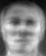
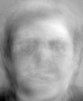
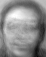
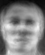
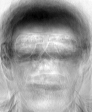
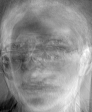
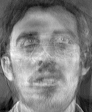
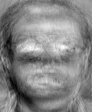
Figure 4: Top five principal components (eigenfaces) for the AT&T Database of Faces. Rows from top to bottom: batch PCA, IPCA, CCIPCA, SGA

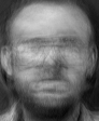
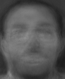
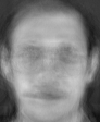
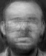
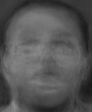
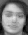
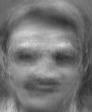
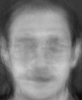
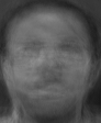
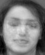
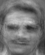
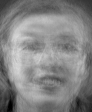
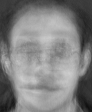
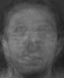
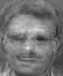
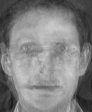
Figure 5: Sample of compressed images from the AT&T Database of Faces ($q=40$ principal components). Rows from top to bottom: original image, batch PCA, IPCA, CCIPCA, SGA

Table 7 displays the classification accuracy of the LDA based on the component scores of the different online PCA algorithms. Overall, all algorithms have high accuracy. IPCA and CCIPCA yields the best performances, followed closely by batch PCA. It is not surprising that online algorithms can surpass batch PCA in classification since the latter technique is only optimal for data compression. SGA produces slightly lower, yet still high classification accuracy.

Table 7: Classification rates for batch PCA, IPCA, CCIPCA, and SGA coupled with Linear Discriminant Analysis on the AT&T Database of Faces

	$q=20$			$q=40$
	Training	Test		Training	Test
Batch	0.9897	0.9580		0.9986	0.9880
IPCA	0.9915	0.9635		0.9995	0.9875
CCIPCA	0.9920	0.9655		0.9988	0.9837
SGA	0.9788	0.9340		0.9963	0.9710

Table 8 examines the computation time and memory usage of the PCA algorithms. As can be expected, batch PCA requires much more (at least one order of magnitude) memory than the online algorithms. Also, the size of the data is large enough so that batch PCA becomes slower than the online algorithms CCIPCA and IPCA. The fact that the SGA algorithm runs slower than all other algorithms is not surprising given that its exact implementation used here requires a Gram-Schmidt orthogonalization in high dimension at each iteration.

Table 8: Computation time (s) and memory usage (MB) for the PCA of the AT&T Database of Faces ($n=400$, $d=10304$).

Method	Time	Memory
Batch PCA	7.13	924.4
IPCA	7.09	73.3
CCIPCA	3.93	74.6
SGA	9.45	67.8

8 Concluding remarks

PCA is a popular and powerful tool for the analysis of high-dimensional data with multiple applications to data mining, data compression, feature extraction, pattern detection, process monitoring, fault detection, and computer vision. We have presented several online algorithms that can efficiently perform and update the PCA of time-varying data (e.g., databases, streaming data) and massive datasets. We have compared the computational and statistical performances of these algorithms using artificial and real data. The R package onlinePCA available at http://cran.r-project.org/package=onlinePCA implements all the techniques discussed in this paper and others.

Of all algorithms under study, the stochastic methods SGA, SNL, and GHA provide the highest computation speed. They are however very sensitive to the choice of the learning rate (or step size) and converge more slowly than IPCA and CCIPCA. For strongly misspecified learning rates, they may even fail to converge. Furthermore, simulations not presented here suggest that a different step size should be used for each estimated eigenvector. In theory this guarantees the almost sure convergence of estimators towards the corresponding eigenspaces (Monnez,, 2006) but, as far as we know, there exist no automatic procedure for choosing these $q$ learning rates in practice. In relation to the recent result given in Balsubramani et al., (2013), averaging techniques (see Polyak and Juditsky, (1992)) could be useful to get efficient estimators of the first eigenvector. Simulation studies not presented here do not confirm at all this intuition. As a matter of fact, averaging improves significantly the initial stochastic gradient estimators when $0.5<\alpha<1$ but the estimation error remains much larger than with IPCA and CCIPCA.

The IPCA and CCIPCA algorithms offer a very good compromise between statistical accuracy and computational speed. They also have the advantage of not having major dependence on tuning parameters (forgetting factor). Approximate perturbation methods can yield highly inaccurate estimates and we do not recommend them in practice. The method of secular equations, although slower than the other algorithms, has the advantage of being exact. It is a very good option when accuracy matters more than speed and the dimension $d$ is not too large. In particular, it is very effective with functional data that have been projected onto a small number of basis functions (FPCA). More generally, when applicable, FPCA should be preferred over standard PCA as it demonstrates both higher accuracy and higher computation speed. In the presence of missing data, imputation procedures like the EBLUP of Brand, (2002) enable online PCA algorithms to continue running without considerable increase in computation time or decrease in accuracy.

For reasons of space, we have focused on rank-1 PCA updates in this paper. However block updates of rank $r\geq 2$ are also frequent in practice. The user choice of the block size $r$ has complex effects on the accuracy and speed of algorithms: for instance, larger blocks tend to reduce noise and estimation variability, but they may also slow down convergence. Regarding computations, as $r$ increases the running time initially decreases but then it reaches a plateau and may even increase if $r$ is too large. In additional simulations (see Supplementary Materials) we examined two online PCA algorithms that allow for block updates: the IPCA algorithm of Levy and Lindenbaum, (2000) and the block-wise stochastic power method of Mitliagkas et al., (2013). In the former algorithm, a rule of thumb is to take $r$ of the same order as the number $q$ of eigenvectors to compute. With the choice $r=q$, this algorithm was actually faster than the fast implementations of the SGA, SNL, and GHA while maintaining the very high accuracy of the rank-1 update IPCA of Section 4. The block-wise stochastic power method was even much faster and, using the recommended block size $r\approx\log(d)/n$, as accurate as the stochastic algorithms.

References

- Arora et al., (2012) Arora, R., Cotter, A., Livescu, K., and Srebo, N. (2012). Stochastic optimization for PCA and PLS. In 50th Annual Conference on Communication, Control, and Computing (Allerton), pages 861–868.
- Ash and Gardner, (1975) Ash, R. and Gardner, M. (1975). Topics in Stochastic Processes. Academic Press, New York.
- Baker et al., (2012) Baker, C., Gallivan, K., and Dooren, P. V. (2012). Low-rank incremental methods for computing dominant singular subspaces. Linear Algebra and its Applications, 436(8):2866 – 2888.
- Balsubramani et al., (2013) Balsubramani, A., Dasgupta, S., and Freund, Y. (2013). The fast convergence of incremental PCA. In NIPS, pages 3174–3182.
- Belhumeur et al., (1997) Belhumeur, P., Hespanha, J., and Kriegman, D. (1997). Eigenfaces vs. fisherfaces: recognition using class specific linear projection. IEEE Trans. Pattern Anal. Mach. Intell., 19(7):711–720.
- Boutsidis et al., (2015) Boutsidis, C., Garber, D., Karnin, Z. S., and Liberty, E. (2015). Online principal components analysis. In Proceedings of the Twenty-Sixth Annual ACM-SIAM Symposium on Discrete Algorithms, SODA 2015, San Diego, CA, USA, January 4-6, 2015, pages 887–901.
- Brand, (2002) Brand, M. (2002). Incremental singular value decomposition of uncertain data with missing values. In ECCV, pages 707–720. Springer-Verlag.
- Budavári et al., (2009) Budavári, T., Wild, V., Szalay, A., Dobos, L., and Yip, C.-W. (2009). Reliable eigenspectra for new generation surveys. Mon. Not. R. Astron. Soc., 394:1496–1502.
- Bunch et al., (1978) Bunch, J. R., Nielsen, C. P., and Sorensen, D. C. (1978). Rank-one modification of the symmetric eigenproblem. Numer. Math., 31(1):31–48.
- Chatterjee, (2005) Chatterjee, C. (2005). Adaptive algorithms for first principal eigenvector computation. Neural Networks, 18(2):145 – 159.
- Duflo, (1997) Duflo, M. (1997). Random iterative models, volume 34 of Applications of Mathematics (New York). Springer-Verlag, Berlin.
- Golub, (1973) Golub, G. H. (1973). Some modified matrix eigenvalue problems. SIAM Review, 15:318–334.
- Golub and Van Loan, (2013) Golub, G. H. and Van Loan, C. F. (2013). Matrix computations. Johns Hopkins Studies in the Mathematical Sciences. Johns Hopkins University Press, Baltimore, MD, fourth edition.
- Gu and Eisenstat, (1994) Gu, M. and Eisenstat, S. (1994). A stable and efficient algorithm for the rank-one modification of the symmetric eigenproblem. SIAM J. Matrix Anal. Appl., 15:1266–1276.
- Halko et al., (2011) Halko, N., Martinsson, P. G., and Tropp, J. A. (2011). Finding structure with randomness: probabilistic algorithms for constructing approximate matrix decompositions. SIAM Rev., 53(2):217–288.
- Hegde et al., (2006) Hegde, A., Principe, J., Erdogmus, D., Ozertem, U., Rao, Y., and Peddaneni, H. (2006). Perturbation-based eigenvector updates for on-line principal components analysis and canonical correlation analysis. J. VLSI Sign. Process., 45:85–95.
- Holmes, (2008) Holmes, S. (2008). Multivariate data analysis: The French way, volume Volume 2 of Collections, pages 219–233. Institute of Mathematical Statistics, Beachwood, Ohio, USA.
- Iodice D’Enza and Markos, (2015) Iodice D’Enza, A. and Markos, A. (2015). Low-dimensional tracking of association structures in categorical data. Stat. Comput., 25(5):1009–1022.
- Jolliffe, (2002) Jolliffe, I. T. (2002). Principal Component Analysis. Springer Series in Statistics. Springer-Verlag, New York, second edition.
- Josse et al., (2011) Josse, J., Pagès, J., and Husson, F. (2011). Multiple imputation in principal component analysis. Adv. Data Anal. Classif., 5(3):231–246.
- Kato, (1976) Kato, T. (1976). Perturbation theory for linear operators. Springer-Verlag, Berlin, second edition.
- Krasulina, (1970) Krasulina, T. (1970). Method of stochastic approximation in the determination of the largest eigenvalue of the mathematical expectation of random matrices. Automat. Remote Control, 2:215–221.
- Lehoucq et al., (1998) Lehoucq, R. B., Sorensen, D. C., and Yang, C. (1998). ARPACK users’ guide, volume 6 of Software, Environments, and Tools. Society for Industrial and Applied Mathematics (SIAM), Philadelphia, PA. Solution of large-scale eigenvalue problems with implicitly restarted Arnoldi methods.
- Levy and Lindenbaum, (2000) Levy, A. and Lindenbaum, M. (2000). Sequential Karhunen-Loeve basis extraction and its application to images. IEEE Trans. Image Process., 9:1371–1374.
- Li et al., (2000) Li, W., Yue, H., Valle-Cervantes, S., and Qin, S. (2000). Recursive PCA for adaptive process monitoring. J. Process Control, 10:471–486.
- Lv et al., (2006) Lv, J. C., Yi, Z., and Tan, K. (2006). Global convergence of Oja’s PCA learning algorithm with a non-zero-approaching adaptive learning rate. Theoret. Comput. Sci., 367(3):286 – 307.
- Mitliagkas et al., (2013) Mitliagkas, I., Caramanis, C., and Jain, P. (2013). Memory limited, streaming PCA. In Burges, C., Bottou, L., Welling, M., Ghahramani, Z., and Weinberger, K., editors, Advances in Neural Information Processing Systems 26, pages 2886–2894. Curran Associates, Inc.
- Monnez, (2006) Monnez, J.-M. (2006). Almost sure convergence of stochastic gradient processes with matrix step sizes. Statist. Probab. Lett., 76(5):531–536.
- Oja, (1983) Oja, E. (1983). Subspace methods of pattern recognition. Research Studies Press.
- Oja, (1992) Oja, E. (1992). Principal components, minor components and linear neural networks. Neural Netw., 5:927–935.
- Oja and Karhunen, (1985) Oja, E. and Karhunen, J. (1985). On stochastic approximation of the eigenvectors and eigenvalues of the expectation of a random matrix. J. Math. Anal. Appl., 106(1):69–84.
- Polyak and Juditsky, (1992) Polyak, B. and Juditsky, A. (1992). Acceleration of stochastic approximation. SIAM J. Control Optim., 30:838–855.
- Ramsay and Silverman, (2005) Ramsay, J.-O. and Silverman, B.-W. (2005). Functional Data Analysis. Springer Series in Statistics, New York, second edition.
- Rao and Principe, (2000) Rao, Y. N. and Principe, J. (2000). A fast, on-line algorithm for PCA and its convergence characteristics. In Neural Networks for Signal Processing X, 2000. Proceedings of the 2000 IEEE Signal Processing Society Workshop, volume 1, pages 299–307.
- Rato et al., (2015) Rato, T., Schmitt, E., De Ketelaere, B., Hubert, M., and Reis, M. (2015). A systematic comparison of PCA-based statistical process monitoring methods for high-dimensional, time-dependent processes. AIChE Journal. Accepted Author Manuscript.
- Sanger, (1989) Sanger, T. D. (1989). Optimal unsupervised learning in a single-layer linear feedforward neural network. Neural Netw., 2:459–473.
- Sibson, (1979) Sibson, R. (1979). Studies in the robustness of multidimensional scaling: perturbational analysis of classical scaling. J. Roy. Statist. Soc. Ser. B, 41(2):217–229.
- Tang et al., (2012) Tang, J., Yu, W., Chai, T., and Zhao, L. (2012). On-line principal component analysis with application to process modeling. Neurocomputing, 82:167–178.
- Wang et al., (2005) Wang, X., Kruger, U., and Irwin, G. W. (2005). Process monitoring approach using fast moving window PCA. Ind. Eng. Chem. Res., 44:5691–5702.
- Warmuth and Kuzmin, (2008) Warmuth, M. K. and Kuzmin, D. (2008). Randomized online PCA algorithms with regret bounds that are logarithmic in the dimension. J. Mach. Learn. Res., 9:2287–2320.
- Weng et al., (2003) Weng, J., Zhang, Y., and Hwang, W.-S. (2003). Candid covariance-free incremental principal component analysis. IEEE Trans. Pattern Anal. Mach. Intell., 25:1034–1040.
- Zha and Simon, (1999) Zha, H. and Simon, H. D. (1999). On updating problems in latent semantic indexing. SIAM J. Sci. Comput., 21(2):782–791 (electronic).
- Zhang and Weng, (2001) Zhang, Y. and Weng, J. (2001). Convergence analysis of complementary candid incremental principal component analysis. Technical Report MSU-CSE-01-23, Department of Computer Science and Engineering, Michigan State University, East Lansing, MI.
- Zhao et al., (2006) Zhao, H., Yuen, P. C., and Kwok, J. T. (2006). A novel incremental principal component analysis and its application for face recognition. IEEE Trans. Syst. Man Cybern. B Cybern., 36:873–886.