Estimating SI violation in CMB due to non-circular beam and complex scan in minutes

Abstract

Mild, unavoidable deviations from circular-symmetry of instrumental beams along with scan strategy can give rise to measurable Statistical Isotropy (SI) violation in Cosmic Microwave Background (CMB) experiments. If not accounted properly, this spurious signal can complicate the extraction of other SI violation signals (if any) in the data. However, estimation of this effect through exact numerical simulation is computationally intensive and time consuming. A generalized analytical formalism not only provides a quick way of estimating this signal, but also gives a detailed understanding connecting the leading beam anisotropy components to a measurable BipoSH characterisation of SI violation. In this paper, we provide an approximate generic analytical method for estimating the SI violation generated due to a non-circular (NC) beam and arbitrary scan strategy, in terms of the Bipolar Spherical Harmonic (BipoSH) spectra. Our analytical method can predict almost all the features introduced by a NC beam in a complex scan and thus reduces the need for extensive numerical simulation worth tens of thousands of CPU hours into minutes long calculations. As an illustrative example, we use WMAP beams and scanning strategy to demonstrate the easability, usability and efficiency of our method. We test all our analytical results against that from exact numerical simulations.

1 Introduction

Observed CMB anisotropy on the sky is a convolution of the underlying cosmological CMB signal with the instrumental beam response function. The instrumental beam (response function) in most CMB experiments are designed to be nearly circularly (azimuthal) symmetric. However, mild deviations from circularity do inevitably arise due to unavoidable limitations in experimental design, function and fabrication; e.g., the primary lobe of the beam exhibits non-circularity due to the off-axis position of detectors on the focal plane; diffraction around the edges of instrument leads to side lobes of the beam; or due to finite response time of detectors, the scan may not correspond to the direction of its beam axis leading to the effective beam response at any pointing direction being sensitive to the scan strategy, etc. Regardless of the specific origin of non-circularity, beam imperfections, coupled with the scan strategy lead to very complex modification of the signal demanding high computational resources to assess the final effect on the estimation of angular power spectrum, cosmological parameters and Statistical Isotropy (SI) violation etc.

Cosmological CMB temperature fluctuations are generally assumed to be a realization of statistically isotropic, Gaussian, correlated random field on the sphere. Consequently, the angular power spectrum has been the primary observational target of most CMB experiments. The effect of NC beam on angular power spectrum of CMB has been studied in literature and the non-trivial impact on high precision cosmological inferences has been appreciated but not satisfactorily resolved, particularly, within the available computational resources. A significant body of literature attempting to deal with NC beam effect on the angular power spectrum exists, e.g.,  [1, 2, 3, 4, 5, 6, 7, 8, 9, 10, 11]. However, current and upcoming CMB experiments also hold the promise to observationally constrain the underlying, often implicit, SI assumption (closely linked to the so called, ‘cosmological principle’), which implies rotational invariance of the $n$-point correlation function. SI assumption has been under intense scrutiny with hints of various ‘anomalies’ persisting in successive years of WMAP data and recently Planck data [12, 13, 14, 15, 16, 17, 18, 19, 20, 21, 22].

Violation of SI can arise both from theoretical possibilities or from observational artefacts [23, 24, 25, 26, 27, 28, 29, 30, 31, 32, 33]. Cosmic topology, anisotropic cosmologies, Doppler boost etc. give some of the theoretical source for SI violation. On the other hand observational artefacts include beam non-circularity, anisotropic noise, foreground residuals, masking etc. Whatever be the source of the SI violation, breakdown of SI can be parametrized by expanding the two point correlation function in the Bipolar Spherical Harmonic (BipoSH) basis [34]. This parametrization captures the SI violation in a mathematically structured representation. NC-beam along with complex scan strategy induces SI violation in an otherwise SI sky and thus pose as a serious systematic contaminant in SI measurements. We use BipoSH basis to characterize the effect.

In this paper, we expand the NC-beam functions in BipoSH basis and the coefficients of expansion are referred as beam-BipoSH coefficients ($B^{LM}_{l_{1}l_{2}}$). An ideal circularly symmetric beam only have $L=0$ non-vanishing beam-BipoSH coefficients. Breakdown of circular symmetry further induces $L\neq 0$ modes in the beam-BipoSH coefficients. Most NC beams have mild deviation from circular symmetry, which reflects as a dominant $m=0$ mode in the beam spherical harmonic coefficients, $b_{lm}$. In most of the realistic beams, $b_{lm}/b_{l0}$ decreases rapidly with increasing m for each $l$. Since, any realistic beam has dominant even-fold symmetry, the odd $m$ modes are also negligible. We provide simple explicit analytic expressions for beam-BipoSH coefficients for any experimental beam and scan. We show that NC-beam introduces the SI violation signals in the measured sky-map such that every non-zero beam-BipoSH coefficient ($B^{LM}_{l_{1}l_{2}}$) generates a corresponding non-zero CMB-BipoSH coefficient ($A^{LM}_{l_{1}l_{2}}$), and analytically relate the beam-BipoSH coefficients with the CMB-BipoSH coefficients for a generalized scan.

Numerical estimation of the BipoSH spectra generated due to experimental beam and scan requires generating multiple realizations of beam convolved CMB maps with the given scan strategy. First step to generate each such realization requires generation of the time order data (TOD) by convolving the random SI sky (generated by HEALPix [35]) with the experimental beam in each time step along the scan path. Thereafter, map-making is used to obtain the realizations from the TOD. This entire process is highly time consuming and computationally expensive. However, our approximate semi-analytic formalism to estimate the effect of mildly NC beam with the experimental scan on the observed CMB-BipoSH coefficients is fast and gives an insight to the corresponding characteristic form of the SI violation. We verify all our analytical results with the results from exact extensive numerical simulations.

The paper is organized as follows. Sec. 2 provides a brief primer to the BipoSH formalism to characterize SI violations for keeping the paper self contained. In Sec. 3, we present a novel expansion of the beam response function in the BipoSH basis. According to our formulation, the beam-BipoSH coefficients depend on the scan pattern. Therefore, in Sec. 3.1 we provide a method for evaluating the beam-BipoSH coefficients in a simplified scan pattern, referred as parallel transport (PT) scan. We provide the detailed expressions for the beam-BipoSH coefficients in PT scan coordinates. In Sec. 4, we derive expressions for the CMB-BipoSH coefficients, arising due to convolution of SI sky-map with a NC-beam, in terms of the beam-BipoSH coefficients. In Sec. 5.1 and Sec. 4, we validate our analytical results against numerical simulations for elliptical Gaussian beam and the WMAP raw beam respectively in a PT scan. Next, in Sec. 5.3 we evaluate the expressions for the CMB-BipoSH coefficients for a generalized scan with NC beam in terms of the CMB-BipoSH coefficients with same beam but PT scan. All these analytical results are verified with numerical simulations. Sec. 6 presents the discussions and conclusions of this paper. Detailed steps of all analytical calculations are provided for completeness in Appendix A and Appendix B.

2 Primer: Bipolar Spherical Harmonic (${\rm BipoSH}$) representation

Statistical Isotropy (SI) implies rotational invariance of $N$-point correlation function and enforces the two point correlation function $C(\hat{n}_{1},\hat{n}_{2})$ to be only a function of the angular separation $(\hat{n}_{1}\cdot\hat{n}_{2})$. Consequently, $C(\hat{n}_{1}\cdot\hat{n}_{2})$ It can be expanded in terms of Legendre polynomials where coefficients of expansion are well known CMB angular power spectrum, $C_{l}$. In harmonic space, this condition translates to diagonal covariance matrix,

$$\langle a_{lm}a^{*}_{l^{\prime}m^{\prime}}\rangle=C_{l}\delta_{ll^{\prime}}\delta_{mm^{\prime}},$$ (2.1)

where $a_{lm}$’s are spherical harmonic coefficients of expansion of CMB temperature field, $\Delta T(\hat{n})$ and the angular bracket denotes the ensemble average. Eq.(2.1) implies that (the $m$-independent), $C_{l}$ encodes all the information in a SI field on the full sky (complete sphere, $\textbf{S}^{2}$).

However, in presence of SI violation the covariance matrix, $\langle a_{lm}a^{*}_{l^{\prime}m^{\prime}}\rangle$ will, in general, have additional terms in the diagonal beyond $C_{l}\delta_{ll^{\prime}}\delta_{mm^{\prime}}$ and also the off-diagonal components. The two point correlation function, then depends on both the directions $\hat{n}_{1}$ and $\hat{n_{2}}$ and not just on the angle between them and most generally can be expanded in Bipolar Spherical Harmonic(BipoSH) basis [34, 36, 37, 38, 39, 40] as

$$C(\hat{n}_{1},\hat{n}_{2})=\sum_{l_{1},l_{2},L,M}A_{l_{1}l_{2}}^{LM}\{Y_{l_{1}}(\hat{n}_{1})\otimes Y_{l_{2}}(\hat{n}_{2})\}_{LM},$$ (2.2)

where $A_{l_{1}l_{2}}^{LM}$ are called the BipoSH coefficients. The bipolar spherical harmonic (BipoSH) functions,

$$\{Y_{l_{1}}(\hat{n}_{1})\otimes Y_{l_{2}}(\hat{n}_{2})\}_{LM}=\sum_{m_{1}m_{2}}C_{l_{1}m_{1}l_{2}m_{2}}^{LM}Y_{l_{1}m_{1}}(\hat{n}_{1})\;Y_{l_{2}m_{2}}(\hat{n}_{2})\,,$$ (2.3)

are irreducible tensor product of two spherical harmonics spaces that form an orthonormal basis on $\textbf{S}^{2}\times\textbf{S}^{2}$. $C_{l_{1}m_{1}l_{2}m_{2}}^{LM}$ are the Clebsch-Gordon coefficients. The multipole indices of these coefficients satisfy the triangularity conditions $|l_{1}-l_{2}|\leq L\leq l_{1}+l_{2}$ and $m_{1}+m_{2}=M$.

We can show that the BipoSH coefficients are given by [34],

$$A^{LM}_{l_{1}l_{2}}=\sum_{m_{1}m_{2}}\langle a_{l_{1}m_{1}}a^{*}_{l_{2}m_{2}}\rangle(-1)^{m_{2}}C^{LM}_{l_{1}m_{1}l_{2}-m_{2}}.$$ (2.4)

The BipoSH coefficients $A^{00}_{ll}$ in Eq.(2.2) corresponds to the SI part and can be expressed in terms of the CMB angular power spectrum as $A^{00}_{ll}=(-1)^{l}C_{l}\prod_{l}$, where $\prod_{ab...c}=\sqrt{(2a+1)(2b+1)...(2c+1)}$ [34].

Non-zero BipoSH coefficients with $L>0$ capture SI violation  [41]. The BipoSH coefficients can be categorized into two distinct classes, defined as even ( $l_{1}+l_{2}+L$ is even) and odd ($l_{1}+l_{2}+L$ is odd) parity BipoSH. This distinction provides valuable clues to the origin of SI violations e.g., weak lensing due to scalar (even parity) and tensor (odd parity) perturbations [42], anisotropic primordial power spectrum (even) [31], temperature modulation (even) [43], primordial homogeneous magnetic fields (even) [44, 30]. Importantly, in the context of NC-beam effect, the absence of significant odd parity BipoSH would imply a reflection symmetric NC-beam.

3 ${\rm Beam-BipoSH}$: Non-circular beams in ${\rm BipoSH}$ representation

Beam function about the pointing direction $\hat{n}$ can be decomposed in Spherical Harmonic (SH) basis as,

$$B(\hat{n},\hat{n}_{1})=\sum_{lm}b_{lm}(\hat{n})Y_{lm}(\hat{n}_{1}).$$ (3.1)

The SH transform of beam at arbitrary pointing direction, $\hat{n}\equiv(\theta,\phi)$ is given by rotating the beam-SH, $b_{lm^{\prime}}(\hat{z})$ – the SH transform of the beam pointing along fixed direction $\hat{z}$,

$$b_{lm}(\hat{n})=\sum_{m^{\prime}}b_{lm^{\prime}}(\hat{z})D^{l}_{mm^{\prime}}(\phi,\theta,\rho(\hat{n})),$$ (3.2)

where Wigner D-functions $D^{l}_{mm^{\prime}}(\alpha,\beta,\gamma)$, are the matrix elements of the rotation operator ($0\leq\alpha<2\pi,\ 0\leq\beta<\pi,\ 0\leq\gamma<2\pi$) and $\alpha,\beta,\gamma$ are the Euler angles that rotate the $\hat{z}$-axis to the pointing direction $\hat{n}=(\theta,\phi)$ and the angle $\rho(\hat{n})$ specifies the orientation of the NC-beam with respect to the local Cartesian coordinates $(\hat{x}\equiv\hat{\phi},\hat{y}\equiv\hat{\theta})$ [1]. Such a rotation can be realized by fixing a coordinate system and performing anti-clockwise rotations, first rotating about the $\hat{z}$-axis by an angle $\alpha=\phi$, then rotating about new $\hat{y}$-axis by an angle $\beta=\theta$, and finally about the new $\hat{z}$-axis by $\gamma=\rho(\hat{n})$.

Since, a general NC-Beam function depends on two vector directions, it can be expanded in the BipoSH basis (see Sec. 2),

$$B(\hat{n},\hat{n}_{1})\ =\sum_{l_{1}l_{2}LM}B^{LM}_{l_{1}l_{2}}\sum_{m_{1}m_{2}}C^{LM}_{l_{1}m_{1}l_{2}m_{2}}Y_{l_{1}m_{1}}(\hat{n})Y_{l_{2}m_{2}}(\hat{n}_{1}),$$ (3.3)

where the coefficients of expansion $B^{LM}_{l_{1}l_{2}}$ are referred to as beam-BipoSH coefficients .

The beam-BipoSH coefficient $B^{LM}_{l_{1}l_{2}}$, can be readily related to beam-SH coefficients $b_{lm}(\hat{n})$ as

$$B^{LM}_{l_{1}l_{2}}=\sum_{m_{1}m_{2}}C^{LM}_{l_{1}m_{1}l_{2}m_{2}}\int d\Omega_{\hat{n}}b_{l_{2}m_{2}}({\hat{n}})Y^{*}_{l_{1}m_{1}}(\hat{n})\,.$$ (3.4)

A circularly symmetric beam function around the pointing direction can be expanded in Legendre polynomials, $B(\hat{n},\hat{n}_{1})\equiv B(\hat{n}\cdot\hat{n}_{1})={(4\pi)}^{-1}\sum_{l}(2l+1)B_{l}P_{l}(\hat{n}\cdot\hat{n}_{1})$. Inverse transforming Eq.(3.3) and using orthogonality of BipoSH [45], we obtain beam-BipoSH coefficients for circularly symmetric beam function,

$$B^{LM}_{l_{1}l_{2}}=(-1)^{l_{1}}B_{l_{1}}\prod_{l_{1}}\delta_{l_{1}l_{2}}\delta_{L0}\delta_{M0},$$ (3.5)

where $B_{l}$ is the commonly used Legendre transform of the beam function in the circularized beam approximation.

Beam-BipoSH depend not only on NC-beam harmonics but also on the scan-strategy that defines $\rho(\hat{n})$, at arbitrary pointing direction, $\hat{n}\equiv(\theta,\phi)$. For any arbitrary scanning strategy, using Eq.(3.2) and Eq.(3.4), it turns out that the beam-BipoSH can be expressed in terms of the beam-SH and scanning parameter $\rho(\hat{n})$ as

$$B^{LM}_{l_{1}l_{2}}\ =\ \sum_{m^{\prime}}b_{l_{2}m^{\prime}}(\hat{z})\Big{(}\sum_{m_{1}m_{2}}C^{LM}_{l_{1}m_{1}l_{2}m_{2}}\ \times\quad\int^{\pi}_{0}\int^{2\pi}_{0}D^{l_{2}}_{m_{2}m^{\prime}}(\phi,\theta,\rho(\hat{n}))Y^{*}_{l_{1}m_{1}}(\hat{n})\sin\theta\leavevmode\nobreak\ d\theta\leavevmode\nobreak\ d\phi\Big{)}.$$ (3.6)

To separate the azimuthal ($\phi$) and polar ($\theta$) dependencies, it is convenient to express Wigner-D functions in terms of Wigner-d through following relation,

$$D^{l}_{mm^{\prime}}(\phi,\theta,\rho(\hat{n}))={\rm e}^{-im\phi}\,d^{l}_{mm^{\prime}}(\theta)\,{\rm e}^{-im^{\prime}\rho(\hat{n})}.$$ (3.7)

Eq.(3.6) is the most general expression of beam-BipoSH coefficients for single hit for any given NC-beam specified through $b_{lm}(\hat{z})$ and scan pattern, defined by $\rho(\theta,\phi)$, in any spherical polar coordinate system (e.g. ecliptic, galactic, etc.).

Analytic progress to evaluate beam-BipoSH coefficients is less tedious when the beam has mild deviations from circularity and allows to retain only the leading order terms up to $|m^{\prime}|=2$ of the beam-SH. Further, in most realistic beam, the beam function has a dominant even fold azimuthal symmetry such that only even values of $m^{\prime}$ is allowed. Hence, throughout the rest of the paper we have truncated the summation over $m^{\prime}$ in Eq.(3.6) with $m^{\prime}=0,\pm 2$. It is worthy to note that $m^{\prime}=0$ is the circular part of the beam. Non-circularity of the beam is characterized by $m^{\prime}=2$. In BipoSH space, the consequence of discrete even-fold azimuthal and reflection symmetric NC-beam translates to restricting non-zero beam-BipoSH to $M=\rm{even}$ and $l_{1}+l_{2}=\textrm{even}$ respectively.

3.1 Beam-BipoSH in ‘Parallel-transport’ scan approximation

The general beam-BipoSH in Eq.(3.6) can be tackled analytically when the scan pattern is such that $\rho(\hat{n})$ is a constant. We refer such a scan pattern as ‘parallel-transport’ (PT) scan following [1]. It implies that the orientation of the beam relative to the local longitude is constant at any point on the sky. Note that a constant $\rho$ can be absorbed as phase factor in the redefinition of the complex quantity $b_{lm}(\hat{z})$ essentially resetting the orientation of the beam (say $\rho(\hat{n})=0$).

In this case, the orthogonality relation,

$$\int^{2\pi}_{0}d\phi\exp(-i(m_{1}+m_{2})\phi)\ =\ 2\pi\,\delta_{m_{1},-m_{2}}\,,$$ (3.8)

implies that the integral over $\phi$ in Eq.(3.6), separates from the integral over $\theta$ and would restrict the non-zero beam-BipoSH to $M=0$,

$$B^{LM}_{l_{1}l_{2}}=\delta_{M0}\frac{2\pi\prod_{l_{1}}}{\sqrt{4\pi}}\sum_{m^{\prime}}b_{l_{2}m^{\prime}}(\hat{z})\times\sum_{m_{2}} (-1)^{m_{2}}C^{L0}_{l_{1}-m_{2}l_{2}m_{2}}I^{l_{1}l_{2}}_{m_{2},m^{\prime}}\,,$$ (3.9)

where

$$I^{l_{1}l_{2}}_{m_{2},m^{\prime}}\ =\ \int d^{l_{2}}_{m_{2}m^{\prime}}(\theta)d^{l_{1}}_{m_{2}0}(\theta)\sin\theta d\theta.$$ (3.10)

Here we use the symmetry property of Wigner-d functions, $d^{l}_{mm^{\prime}}=(-1)^{m-m^{\prime}}d^{l}_{-m-m^{\prime}}$.

To make analytical progress, we need to evaluate $I^{l_{1}l_{2}}_{m_{2},m^{\prime}}$ for $m^{\prime}=-2,0,2$ (as already discussed for all other $m^{\prime}$ modes $b_{l_{2}m^{\prime}}$ are negligable). It is important to note that, circular part of beam function $m^{\prime}=0$ will show up as $L=0$ mode in beam-BipoSH coefficient. The non-circular $m^{\prime}=\pm 2$ part of the beam will give rise to non-trivial ($L\neq 2$) beam-BipoSH.

• beam-BipoSH due to $m^{\prime}=0$ mode of beam function:

  For $m^{\prime}=0$, $I^{l_{1}l_{2}}_{m_{2},m^{\prime}}$ in Eq.(3.9) can be simplified to,

  $$I^{l_{1}l_{2}}_{m_{2},0} = \frac{2}{2l_{2}+1}\delta_{l_{1}l_{2}}.$$ (3.11)

  Therefore, beam-BipoSH coefficients for circular part of the beam are of following form (refer Appendix B),

  $$B^{LM}_{l_{1}l_{2}} = (-1)^{l_{2}}b_{l_{2}0}(\hat{z})\sqrt{4\pi}\delta_{l_{1}l_{2}}\delta_{L0}\delta_{M0}\delta_{m^{\prime}0}.$$ (3.12)

• beam-BipoSH due to $m^{\prime}=\pm 2$ mode of beam function:

  For $m^{\prime}=\pm 2$, the integrals are evaluated separately for the $m_{2}=0$ and $m_{2}\neq 0$ parts of the summation. In the former case when $m_{2}=0$ and $m^{\prime}=\pm 2$, the integral in Eq.(3.10) simplifies to,

  $$I^{l_{1}l_{2}}_{0,\pm 2}\ =\ \quad\left\{\begin{array}[]{ll}0&\mbox{if ($l_{1}+l_{2}\equiv\textrm{odd}$)}\\ 0&\mbox{if ($l_{1}>l_{2}$)}\\ 4\sqrt{\frac{(l_{2}-2)!}{(l_{2}+2)!}}&\mbox{if ($l_{1}<l_{2}$)}\\ \sqrt{\frac{(l_{2}-2)!}{(l_{2}+2)!}}\big{[}\frac{4l_{2}}{(2l_{2}+1)}-\frac{2l_{2}(l_{2}+1)}{(2l_{2}+1)}\big{]}&\mbox{if ($l_{1}=l_{2}$)}\,.\end{array}\right.$$ (3.17)

  For $m_{2}\neq 0$, $d^{l_{2}}_{m_{2}\pm 2}(\theta)$ is recursively expanded in terms of $d^{l_{2}}_{m_{2}0}(\theta)$ to evaluate $I^{l_{1}l_{2}}_{m_{2},\pm 2}$ (refer Appendix B). NC beam with reflection symmetry have non-vanishing beam-BipoSH with even-parity. Hence, the beam-BipoSH due to the NC part of the beam in the PT-scan approximation is of the following form, only,

  $$B^{LM}_{l_{1}l_{2}}=\delta_{M0}\frac{2\pi\prod_{l_{1}}}{\sqrt{4\pi}}\left(b_{l_{2}2}(\hat{z})+b^{*}_{l_{2}2}(\hat{z})\right)\left[C^{L0}_{l_{1}0l_{2}0}I^{l_{1}l_{2}}_{0,2}+\sum_{m_{2}\neq 0}(-1)^{m_{2}}C^{L0}_{l_{1}-m_{2}l_{2}m_{2}}I^{l_{1}l_{2}}_{m_{2},2}\right]\,.$$ (3.18)

  For a PT scan, beam-BipoSH encodes the effect of NC beam $b_{l_{2}2}(\hat{z})$ in the second part of the expression.

The above expression for beam-BipoSH coefficient holds for the PT-scan (with constant $\rho({\hat{n}})$) for a NC-beam that has reflection symmetry. Although we have restricted explicit analytic results presented in the text to reflection symmetric beam functions, in general, odd parity beam BipoSH will be non-vanishing in absence of the above mentioned symmetries. Appendix B provides expressions for odd-Parity beam-BipoSH $B^{LM^{(-)}}_{l_{1}l_{2}}$, that can be used as a measure of breakdown of reflection symmetry in NC beam. Note that the BipoSH estimator [43], that differ by a factor from original definition of Hajian & Souradeep [34, 40], used by the WMAP team cannot be extended to odd-parity BipoSH, However, it is possible to devise BipoSH estimators that can measure odd-parity BipoSH spectra while matching that employed by WMAP for even-parity BipoSH spectra [46].

4 Relating ${\rm beam-BipoSH}$ with ${\rm CMB-BipoSH}$

The measured CMB temperature is the convolution of true underlying CMB temperature with the instrument beam,

$$\widetilde{\Delta T}(\hat{n}_{1})=\int d{\Omega_{\hat{n}_{2}}}B(\hat{n}_{1},\hat{n}_{2})\Delta T(\hat{n}_{2}).$$ (4.1)

Here, $\Delta T(\hat{n}_{2})$ is the underling true sky temperature along $\hat{n}_{2}$ and $\widetilde{\Delta T}(\hat{n}_{1})$ is the temperature measured along $\hat{n}_{1}$. $B(\hat{n}_{1},\hat{n}_{2})$ is known as the beam response function and gives the sensitivity of the detector around the pointing direction, $\hat{n}_{1}$. The observed two point correlation function is,

$$\tilde{C}(\hat{n}_{1},\hat{n}_{2})\equiv\langle\widetilde{\Delta T}(\hat{n}_{1})\widetilde{\Delta T}(\hat{n}_{2})\rangle\ =\int d\Omega_{n}\int d\Omega_{n^{\prime}}C(\hat{n}^{\prime},\hat{n})B(\hat{n}_{1},\hat{n}^{\prime})B(\hat{n}_{2},\hat{n}),$$ (4.2)

where $C(\hat{n}^{\prime},\hat{n})=\langle\Delta T(\hat{n}^{\prime})\Delta T(\hat{n})\rangle$, is the underlying correlation function. It is evident from Eq.(4.2), that SI violation can occur either due to breakdown of rotational invariance of the underlying correlation function $C(\hat{n}_{1},\hat{n}_{2})\not\equiv C(\hat{n}_{1}\cdot\hat{n}_{2})$, or due to the breakdown of circularity in beam response function $B(\hat{n}_{1},\hat{n}_{2})\not\equiv B(\hat{n}_{1}\cdot\hat{n}_{2})$, or both.

Inverse transform of Eq.(2.2), yields the most general for CMB-BipoSH coefficients $\tilde{A}^{LM}_{l_{1}l_{2}}$,

$$\tilde{A}^{LM}_{l_{1}l_{2}} = \int d\Omega_{n_{1}}\int d\Omega_{n_{2}}\tilde{C}(\hat{n}_{1},\hat{n}_{2})\{Y_{l_{1}}(\hat{n}_{1})\otimes Y_{l_{2}}(\hat{n}_{2})\}^{*}_{LM}$$ (4.3)

which under PT scan of an underlying isotropic sky becomes (Appendix A)

$$\tilde{A}^{LM}_{l_{1}l_{2}}\ =\ \sum_{l}(-1)^{l}C_{l}\sum_{L_{1}M_{1}L_{2}M_{2}}B^{L_{1}M_{1}}_{l_{1}l}B^{L_{2}M_{2}}_{l_{2}l}\ \times\prod_{L_{1}L_{2}}C^{LM}_{L_{1}M_{1}L_{2}M_{2}}{\begin{Bmatrix}l&l_{2}&L_{2}\\ L&L_{1}&l_{1}\end{Bmatrix}}\,.$$ (4.4)

The equations shows that provided the beam-BipoSH coefficients ($B^{LM}_{ll^{\prime}}$) are restricted to $M=0$, the corresponding BipoSH coefficients of the CMB maps are also restricted to $M=0$. It also turns out that due to triangularity condition ($|L_{1}-L_{2}|\leq L\leq L_{1}+L_{2}$), the most dominant terms in the above summation are $\{L_{1}=L,L_{2}=0\}\ \textrm{and}\ \{L_{1}=0,L_{2}=L\}$ as they are proportional to $B^{00}_{l_{1}l}B^{L0}_{l_{2}l}$ and $B^{L0}_{l_{1}l}B^{00}_{l_{2}l}$. The product of these two beam-BipoSH coefficients in turn depends on the product of SH coefficients $b_{l0}b_{l2}$. In a mildly non-circular beam response function $b_{l0}$, is significantly larger than $b_{l2}$, making $b_{l0}b_{l2}$ much larger than $b_{l2}b_{l2}$, which will contribute as second order terms in Eq.(4.4).

The BipoSH estimator used by the WMAP team [47, 43], differs from our defination (the original BipoSH definition in Hajian & Souradeep [34]) by a factor of ${\prod_{L}}/({\prod_{l_{1}l_{2}}C^{L0}_{l_{1}0l_{2}0})}$ and are restricted to only even-parity BipoSH 

$$\tilde{A}^{L0^{\rm WMAP}}_{l_{1}l_{2}}=\frac{\prod_{L}}{\prod_{l_{1}l_{2}}C^{L0}_{l_{1}0l_{2}0}}\tilde{A}^{L0}_{l_{1}l_{2}}\,.$$ (4.5)

SI violation signals in WMAP-7 were measured in two BipoSH spectra, $A^{20}_{ll}$ and $A^{20}_{l-2l}$, we provide explicit leading order expressions for these coefficients arising from the NC-beam as,

$$\tilde{A}^{20^{\rm WMAP}}_{ll} = \frac{(-1)^{l}\,2\sqrt{5}\,C_{l}\,B^{00}_{ll}B^{20}_{ll}}{(\prod_{l})^{3}C^{20}_{l0l0}}\,,$$ (4.6)

$$\tilde{A}^{20^{\rm WMAP}}_{l-2l} = \frac{\sqrt{5}(-1)^{l}}{\prod_{{l-2}l}C^{20}_{{l-2}0l0}}\ \times\ \Big{[}\frac{C_{l-2}B^{00}_{{l-2}{l-2}}B^{20}_{l{l-2}}}{\prod_{l-2}}+\frac{C_{l}B^{00}_{ll}B^{20}_{{l-2}l}}{\prod_{l}}\Big{]}\,.$$ (4.7)

Note, that BipoSH expression in Eq.(4.6) and Eq.(4.7) are provided in the scaled form that matches the BipoSH estimator employed by the WMAP team. The BipoSH spectra plotted in different figures in this paper are in accordance with WMAP definition.

5 Analytical evalution of ${\rm CMB-BipoSH}$ coefficients

5.1 Elliptical Gaussian beam in PT scan

Elliptical-Gaussian (EG) functions provide a simple model of NC-beam as an extension to the often used circular-symmetric Gaussian beam function. BipoSH coefficients obtained from EG beams serve to crosscheck and validate analytical expression derived in Eq.(3.9), Eq.(4.6) and Eq.(4.7), and puts a check on the numerical simulation of CMB maps convolved (in real space) with an NC-beam (full details of numerical simulations can be found in [19, 10]).

An EG-beam function pointed along $\hat{z}$ axis can be expressed in spherical polar coordinates, as

$$B(\hat{z},\hat{n})\ =\ \frac{1}{2\pi\sigma_{1}\sigma_{2}}\exp\left[-\frac{{\theta^{2}}}{2\sigma^{2}(\phi)}\right],$$ (5.1)

where the azimuth angle dependent beam-width $\sigma(\phi_{1})\ \equiv\ [\sigma_{1}^{2}/(1+\epsilon\sin^{2}\phi_{1})]^{1/2}$ is given by Gaussian widths $\sigma_{1}$ and $\sigma_{2}$ along the semi-major and semi-minor axes. The non-circularity parameter $\epsilon\ =\ (\sigma_{1}^{2}/\sigma_{2}^{2}-1)$, which is related to eccentricity $e=\sqrt{1-\sigma_{2}^{2}/\sigma_{1}^{2}}$. As expected, the EG beam reduces to circular Gaussian beam for zero eccentricity ($e=0$). Higher the value of eccentricity, stronger the deviation from circularity. An analytical expression for the beam-SH of EG-beam is available in [1]. Due to even-fold azimuthal symmetry and reflection symmetry, $b_{lm}(\hat{z})=0$, for odd $m$; and for even $m$,

$$b_{lm}(\hat{z})\ \ =\ \ \sqrt{\frac{(2l+1)(l+m)!}{4\pi(l-m)!}}(l+\frac{1}{2})^{-m}\ \times$$

$$\quad I_{m/2}\Bigg{[}(l+\frac{1}{2})^{2}\frac{\sigma^{2}_{1}e^{2}}{4}\Bigg{]}\exp\big{[}{-(l+\frac{1}{2})^{2}\frac{\sigma^{2}_{1}}{2}({1-\frac{e^{2}}{2}})\big{]}}\,,$$

where $I_{\nu}(x)$ is the modified Bessel function. The reality condition of beam, $b^{*}_{lm}=b_{lm}$ for even $m$, then implies $b_{l-m}=b_{lm}$.

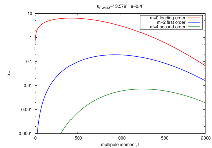
Figure 1: The coefficients of spherical harmonic expansion of an EG beam with $\theta_{\rm{FWHM}}=13.579^{\prime}$ and eccentricity $e=0.4$. The circular symmetric component of the beam, given by $m=0$ is the dominating term. The next leading contribution comes from $m=2$ mode which gives the effect of non-circularity of the beam. The higher $m$ modes are negligible.

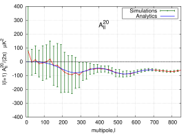
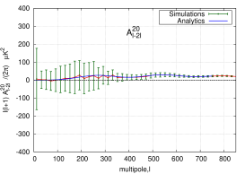
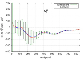
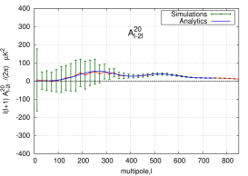
Figure 2: BipoSH spectra $A^{20}_{ll}$ and $A^{20}_{l-2l}$ for EG beam with : (Top) $\theta_{\rm{FWHM}}=13.579^{\prime}$ and eccentricity $e=0.4$; (Bottom) $\theta_{\rm{FWHM}}=17.7036^{\prime}$ and eccentricity $e=0.46$. Smooth (blue) curve are CMB-BipoSH computed using the analytic expressions. The red curve with corresponding error-bars are obtained from 100 numerical simulated SI maps convolved with the same EG beam.

For EG beams, the ratio $b_{lm}/b_{l0}$ dies down rapidly with $|m|$. In Fig. 1, we plot beam-SH coefficients of an EG beam with $\theta_{\rm{FWHM}}=13.579^{\prime}$ and eccentricity $e=0.4$, which is close to an elliptical estimate of W band beam of WMAP. The plot clearly shows that the $m=4$ mode is negligible in compared to $m=2$ mode. We will also get similar feature if we consider an EG-beam with $\theta_{\rm{FWHM}}=17.7036^{\prime}$ with eccentricity $e=0.46$ which is close to the V-band beam. Therefore, for our analysis we restrict our calculations to $m=0,\pm 2$ modes. We estimate beam-BipoSH coefficient in Eq.(3.9) for PT scan by using the closed analytical form of $b_{lm}$’s as in Eq.(5.1). Finally, using Eq.(4.6) and Eq.(4.7), we obtain the CMB BipoSH spectra $A^{20}_{ll}$ and $A^{20}_{l-2l}$. We verify our analytical results with BipoSH coefficients evaluated from $100$ SI maps numerically convolved with EG-beam functions (see Fig. 2).

5.2 WMAP raw beam with PT scan

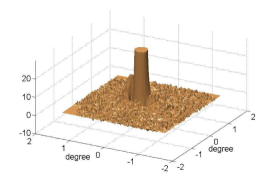
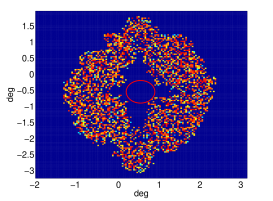
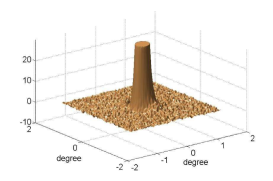
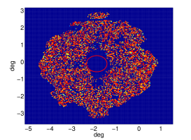
Figure 3: Beam response function of A side of W1 differencing assembly (Top) and A side of V2 differencing assembly (Bottom) are shown. The Left-hand panels show 3D zoomed view of the central part of the beam. The central part is truncated to highlight the features existed in the elliptical contour. The Right-hand panels cover the entire beam-map images to show the spread-out annular distribution of regions with negative response. (The red circles marks the central beam peak region). The power in negative response is $\sim 0.5$ of the positive power in the central peak. The annular negative power distribution shows quadrupolar feature that modifies the beam-SH $b_{l2}$ to take negative values at high $l$ (see Fig 5). It is apparent then that correctly accounting for WMAP NC-beam effects numerically, requires the convolution of the entire beam map region with the SI sky-map leading to enormous increase in computing costs (relative to using only the central peak).

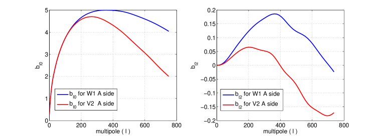
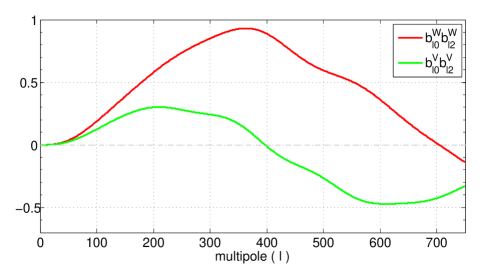
Figure 4: Top: Beam spherical harmonic transforms, $b_{l0}$ and $b_{l2}$ of beam maps of A side of W1 and V2 DA.
Bottom: The plot of the NC-beam leading order NC beam perturbation parameter $b_{l0}b_{l2}$ vs. $l$ . The plots show that although BipoSH peak structure is largely set by the underlying angular power spectrum $C_{l}$ of SI cosmological mode, small differences observed at the two different frequencies can arise because of the difference in the shapes of $b_{l0}b_{l2}$.

It is widely-known that the WMAP beams are non-circular and deviate from a Gaussian profile and that an EG beam is not a good approximation [48, 3, 49]. WMAP-7 year data had a whopping SI violation detection in $A^{20}_{ll}$ and $A^{20}_{ll-2}$ BipoSH coefficients [47]. Later on it was realized that it was due to the noncircularity of the WMAP beams which was corrected in the WMAP-9 year data. No such signal is observed in Planck data which reinforce the fact that it was due to the particular shape of the beam and the scan pattern.

To see the imprint of the WMAP kind of beam on the BipoSH coefficients, we consider the A side raw beam maps of the V2 and W1 differencing Assembly (DA) of WMAP as representative of the V and W band beams, respectively (see Fig. 3). The central part of the beam maps show an elliptical peak with non-trivial ‘shoulder-like’ features. Apart from this, the beam functions contain an annular region with positive and negative sensitivity spread over a diameter of $3^{\circ}$ to $5^{\circ}$. In the right-hand panels, we highlight the regions with negative response. The integrated power in the negative beam response is $\sim 0.5$ of the total power.

We compute the beam-SH coefficients for these assemblies numerically to use in semi-analytic estimate of the CMB-BipoSH coefficients, using Eq.(4.6) and Eq.(4.7). Fig. 4 is a plot of the $b_{l0}$ and leading order $b_{l2}$ beam-SH coefficients of the W1A and V2A raw beam maps. Note that the $b_{l2}$ spectrum changes sign and takes negative values at high $l$ – a key qualitative feature of the WMAP beams. The origin of this curious feature is the negative responce of the beam sensitivity function as seen in the right hand panel of the Fig. 3. This particular feature cannot be captured in Elliptical-Gaussian beam model where $b_{l2}$ does not change sign with $l$. This peculiar nature of $b_{l2}$ reflects as flipping of sign in $A^{20}_{ll}$ spectra of V-band at high $l$ as seen in the WMAP-7 measurements. Such a unique correspondence between a beam-SH feature and the consequent CMB-BipoSH is unlikely to be mimicked by other effects and has been confirmed independently by various authors that WMAP seven year SI violation detection was due to NC Beam.

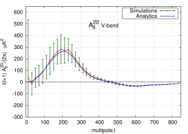
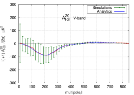
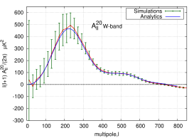
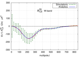
Figure 5: BipoSH spectra, $A^{20}_{ll}$ (Left) and $A^{20}_{l-2l}$ (Right) obtained for the raw beam maps A side of V2 channel (Top) and A side of W1 channel (Bottom) of the WMAP experiment. Analytically evaluated BipoSH spectra (blue) overlaid on the average BipoSH spectra (red) with error bars obtained from 100 simulations of statistically isotropic CMB sky convolved W1 and V2 channel of WMAP.

We use PT-scan in ecliptic coordinates to get an estimate of $A^{20}_{ll}$ and $A^{20}_{ll-2}$ due to NC Beam. This particular coordinate system is chosen because WMAP scan is azimuthally symmetric around ecliptic pole. We verify our analytical results using BipoSH coefficients from the numerical simulations where we generate non-SI maps by numerically convolving the WMAP W1A and V2A beam with the SI maps (see Fig. 5).

Here we list some of the key features that we see in the results :

1. From our analytical understanding, which is also verified by numerical simulations, in a coordinate system where PT scan is valid, only $M=0$ should be significant.

2. We notice the NC beam effect is larger in W band than in V band explaining the difference in detected SI violation signal at the two frequencies.

3. The BipoSH spectra $A^{20}_{ll}$, $A^{20}_{ll-2}$ changes sign at large $l$ (in V-band its more prominent). This happens because the beams contains the negative sensitivity region in the annular part leading to a sign flip in $b_{l2}$ at high $l$.

4. The BipoSH coefficients from NC beam shows a prominent bump roughly around the first acoustic peak ($l=220$) for both W and V band. This corresponds mainly to the scale picked by the underlying angular power spectrum $C_{l}$. However, the precise peak location also depends on the peak in $b_{l0}b_{l2}$ for each band and can account for differences in the peak location in the two bands shown in Fig. 4.

5.3 WMAP raw beam and scan strategy

The WMAP satellite follows a differential scan strategy where it records the temperature difference between two telescopic horns for each frequency band. The pair of horns are about $70.5^{\circ}$ off the satellite’s symmetry axis. It spins with a spin period of around 2.2 minutes about the symmetric axis. Along with this the spacecraft also has a slow precession, $22.5^{\circ}$ about the Sun-WMAP line. Precession period is about 1 hour. The satellite orbits around the sun with a period of a year [10].

The differential scan pattern is mostly used to reduce the noise in the observed data. However, for evaluating an analytical estimate of the BipoSH coefficients for the real scan, we make the following assumptions :

• We assume the beams in the A side and B side of the differential assembly are identical.

• The observed temperature of a pixel is the average of all the hits on that pixel from any orientation of the beam ( irrespective of A or B side ).

The effect of non-circular beam on sky map is sensitive to the scan-strategy. The effective beam that convolves the true sky resulting in the observed sky map is created by an intricate combination of the instantaneous beam of the instrument and the scan strategy. Every time the beam hits a particular pixel, the beam BipoSH coefficient is given by Eq.(3.6). The beam visits the same pointing direction ($\hat{n}^{\prime}$) multiple times with different orientations $\rho_{{\hat{n}^{\prime}},j}$, where $\rho_{{\hat{n}^{\prime}},j}$ is the orientation of the beam at the $j^{\rm th}$ hit. The Beam BipoSH coefficients for this case can be expressed as

$$B^{LM}_{l_{1}l_{2}}(\hat{n}^{\prime},j,\hat{z})=\sum_{m^{\prime}}b_{l_{2}m^{\prime}}(\hat{z})\Big{(}\sum_{m_{1}m_{2}}C^{LM}_{l_{1}m_{1}l_{2}m_{2}}\int\exp^{-im_{2}\phi}d^{l_{2}}_{m_{2}m^{\prime}}(\theta)\exp^{-im^{\prime}\rho_{\hat{n}^{\prime},j}}Y^{*}_{l_{1}m_{1}}(\hat{n})\leavevmode\nobreak\ d\hat{n}\leavevmode\nobreak\ \Big{)}\,.$$ (5.3)

Here $\hat{z}$ denotes the direction along which the beam is expanded in the spherical harmonics and the beam-BipoSH coefficients are calculated. In case of PT scan, as the beam visits different pixels with same orientation all the time, $\rho_{{\hat{n}^{\prime}},j}$ = constant, which makes the BipoSH coefficient independent of the direction (${\hat{n}^{\prime}}$), which is not true in general, as seen in the above equation. The orientation of the beam for different directions ($\hat{n}^{\prime}$) at different time ($j$) will be different. Therefore, the beam-BipoSH becomes a function of the direction $\hat{n}^{\prime}$ and time of scan $j$. As $\rho_{\hat{n}^{\prime},j}$ is independent of $\hat{n}$ it comes out of the integral.

Suppose the beam hits the $\hat{n}^{\prime}$ direction, $n_{\hat{n}^{\prime}}$ times. As we assume that the temperatures along $\hat{n}$ direction are averaged over all the measurements, we can consider the beam along $\hat{n}^{\prime}$ direction as an average of beams in all the hits. Then the average beam-BipoSH can be expressed as

$$\bar{B}^{LM}_{l_{1}l_{2}}(\hat{n}^{\prime},\hat{z}) = \sum_{m^{\prime}}\chi_{m^{\prime}}(\hat{n}^{\prime})b_{l_{2}m^{\prime}}(\hat{z})\Big{(}\sum_{m_{1}m_{2}}C^{LM}_{l_{1}m_{1}l_{2}m_{2}}\times\int\exp^{-im_{2}\phi}d^{l_{2}}_{m_{2}m^{\prime}}(\theta)Y^{*}_{l_{1}m_{1}}(\hat{n})\leavevmode\nobreak\ d\hat{n}\leavevmode\nobreak\ \Big{)}$$ (5.4)

$$= \sum_{m^{\prime}}\left(\sum_{lm}f^{(m^{\prime})}_{lm}Y_{lm}(\hat{n}^{\prime})\right){\mathcal{B}}^{LM^{({m^{\prime}})}}_{l_{1}l_{2}}(\hat{z})\,,$$

where $\chi_{m^{\prime}}(\hat{n}^{\prime})=\frac{1}{{n_{\hat{n}^{\prime}}}}{\sum_{j}\left(\exp^{-im^{\prime}\rho_{\hat{n}^{\prime},j}}\right)}$. Since for each $m^{\prime}$ mode, $\chi_{m^{\prime}}(\hat{n}^{\prime})$ is a function of $\hat{n}^{\prime}$, we expand them in the spherical harmonics (see Eq.(5.4)). ${\mathcal{B}}^{LM^{({m^{\prime}})}}_{l_{1}l_{2}}(\hat{z})$ would be the beam-BipoSH coefficients if only one $m^{\prime}$ mode of the beam was non zero with PT scan.

The $\hat{n}^{\prime}$ direction of the sky is now scanned by a beam with beam-BipoSH coefficient $\bar{B}^{LM}_{l_{1}l_{2}}(\hat{n}^{\prime},\hat{z})$. Therefore, substituting Eq.(5.4) into Eq.(A.5) the coefficients of the spherical harmonics of the scanned sky-map turns out to be

$$\tilde{a}_{JK}=\sum_{l_{1}m_{1}lmLM\bar{l}\bar{m}}\left(-1\right)^{m}\frac{\Pi_{\bar{l}}\Pi_{l_{1}}}{\sqrt{4\pi}\Pi_{j}}\sum_{m^{\prime}}{\mathcal{B}}_{l_{1}l}^{LM^{(m^{\prime})}}f_{\bar{l}\bar{m}}^{(m^{\prime})}C_{l_{1}m_{1}l-m}^{LM}C_{\bar{l}0l_{1}0}^{J0}C_{\bar{l}\bar{m}l_{1}m_{1}}^{JK}a_{lm}\,.$$ (5.5)

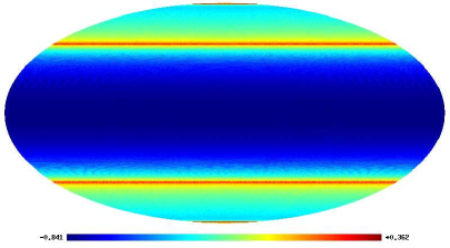
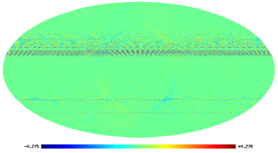
Figure 6: Map of $\langle\cos(2\rho)\rangle$ and $\langle\sin(2\rho)\rangle$ in ecliptic coordinate for full year WMAP scan. The angular bracket ( $\langle\,\dots\,\rangle$ ) denotes average over all the hits on a pixel irrespective of beam from A-side or B-side differential assambly of WMAP satellite. Its important to note that $\langle\sin(2\rho)\rangle$ is almost $0$ in all the pixels.

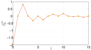
Figure 7: Spherical harmonics of a $\cos{2\rho}$ map of WMAP scan are significantly dominated by $m=0$ modes. This is expected as WMAP scan is azimuthally symmetric in ecliptic coordinates. Also, the amplitude of SH coefficients of $\cos{2\rho}$ map decreases with increasing multipoles $l$ and having negligible contribution from odd multipoles $l$. As can be seen in above figure, $l=0$ and $l=2$ modes are most dominant and are used for analytical estimation effect of scan on beam-BipoSH. Nevertheless, the effect of scanning strategy can be evaluated by taking all significant SH coefficients into account for any experiment.

The above equation gets simplified under the following assumptions :

• The only dominant modes of $b_{l_{2}m^{\prime}}(\hat{z})$ in Eq.(5.4) for the WMAP beam are the $|m^{\prime}|=0,\ 2$ modes (see Sec. 4). Therefore, only ${\mathcal{B}}_{l_{1}l}^{LM^{(m^{\prime})}}$ with $m^{\prime}=0,\pm 2$ will contribute to the above equation. Since the imaginary part of $\chi_{2}(\hat{n}^{\prime})$ is zero (see Fig. 6), it implies $\chi_{2}(\hat{n}^{\prime})=\chi_{-2}(\hat{n}^{\prime})$.

• The WMAP scan pattern is azimuthally symmetric about ecliptic pole axis. Therefore, in the ecliptic coordinate we can assume $f_{\bar{l}\bar{m}}=0$ for all $\bar{m}\neq 0$.

Under these assumptions Eq.(5.5) simplifies to

$$\tilde{a}_{JK}=\sum_{l_{1}\bar{l}}\frac{\Pi_{\bar{l}}\Pi_{l_{1}}}{\sqrt{4\pi}\Pi_{J}}C_{\bar{l}0l_{1}0}^{J0}C_{\bar{l}0l_{1}K}^{JK}\left(\tilde{\mathfrak{A}}_{l_{1}K}^{(c)}f_{\bar{l}0}^{(0)}+\tilde{\mathfrak{A}}_{l_{1}K}^{(nc)}f_{\bar{l}0}^{(2)}\right)$$ (5.6)

where,

$$\tilde{\mathfrak{A}}_{l_{1}m_{1}}^{(c)} = \sum_{lmLM}\left(-1\right)^{m}a_{lm}{\mathcal{B}}_{l_{1}l}^{LM^{(0)}}C_{l_{1}m_{1}l-m}^{LM}=\sum_{lm}\frac{\left(-1\right)^{m}}{\sqrt{2l+1}}a_{lm}{\mathcal{B}}_{ll}^{00}\,,$$ (5.7)

$$\tilde{\mathfrak{A}}_{l_{1}m_{1}}^{(nc)} = \sum_{lmLM}\sum_{m^{\prime}=2,-2}\left(-1\right)^{m}a_{lm}{\mathcal{B}}_{l_{1}l}^{LM^{(m^{\prime})}}C_{l_{1}m_{1}l-m}^{LM}\,.$$ (5.8)

$\tilde{\mathfrak{A}}_{l_{1}m_{1}}^{(c)}$, $\tilde{\mathfrak{A}}_{l_{1}m_{1}}^{(nc)}$ are the coefficients of the spherical harmonics of a sky convolved with the circular and the non-circular part of the beam respectively, using PT scan. Beam-BipoSH coefficients as obtained from the circular part of the beam ($m^{\prime}=0$) i.e. ${\mathcal{B}}_{l_{1}l}^{LM^{(0)}}$ are non vanishing only for $L=0$. Similarly the beam-BipoSH coefficients obtained from the non-circular part of the beam ($m^{\prime}\neq 0$) are non zero only for $L\neq 0$. Since the deviation from circularity is mild, ${\mathcal{B}}_{l_{1}l}^{LM^{(0)}}$ will be dominant as compared to ${\mathcal{B}}_{l_{1}l}^{LM^{(m^{\prime}\neq 0)}}$.

Using Eq.(5.6), the BipoSH coefficients from the scanned sky can be obtained as

$$\tilde{A}_{l_{1}l_{2}}^{L^{\prime}M^{\prime}} = \sum_{m_{1}m_{2}}\left\langle\tilde{a}_{l_{1}m_{1}}\tilde{a}_{l_{2}m_{2}}\right\rangle C_{l_{1}m_{1}l_{2}m_{2}}^{L^{\prime}M^{\prime}}$$ (5.9)

$$= \sum_{m_{1}m_{2}}\sum_{l\bar{l}}\sum_{l^{\prime}\bar{l}^{\prime}}\frac{\Pi_{\bar{l}}\Pi_{l}\Pi_{\bar{l}^{\prime}}\Pi_{l^{\prime}}}{4\pi\Pi_{l_{1}}\Pi_{l_{2}}}C_{\bar{l}0l0}^{l_{1}0}C_{\bar{l}0lm_{1}}^{l_{1}m_{1}}C_{\bar{l}^{\prime}0l^{\prime}0}^{l_{2}0}C_{\bar{l}^{\prime}0l^{\prime}m_{2}}^{l_{2}m_{2}}\times\left[\left\langle\tilde{\mathfrak{A}}_{lm_{1}}^{(c)}\tilde{\mathfrak{A}}_{l^{\prime}m_{2}}^{(c)}\right\rangle f_{\bar{l}0}^{(0)}f_{\bar{l}^{\prime}0}^{(0)}\right.$$

$$\left.+\left\langle\tilde{\mathfrak{A}}_{lm_{1}}^{(nc)}\tilde{\mathfrak{A}}_{l^{\prime}m_{2}}^{(c)}\right\rangle f_{\bar{l}0}^{(2)}f_{\bar{l}^{\prime}0}^{(0)}+\left\langle\tilde{\mathfrak{A}}_{lm_{1}}^{(c)}\tilde{\mathfrak{A}}_{l^{\prime}m_{2}}^{(nc)}\right\rangle f_{\bar{l}0}^{(0)}f_{\bar{l}^{\prime}0}^{(2)}+\left\langle\tilde{\mathfrak{A}}_{lm_{1}}^{(nc)}\tilde{\mathfrak{A}}_{l^{\prime}m_{2}}^{(nc)}\right\rangle f_{\bar{l}0}^{(2)}f_{\bar{l}^{\prime}0}^{(2)}\right]\,.$$

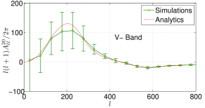
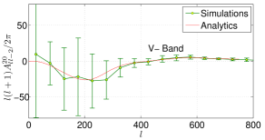
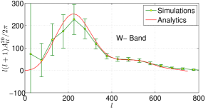
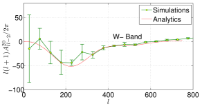
Figure 8: BipoSH spectra, $A^{20}_{ll}$ (Left) and $A^{20}_{l-2l}$ (Right) obtained for the raw beam maps A side of V2 channel (Top) and A side of W1 channel (Bottom) of the WMAP experiment for the WMAP scan strategy. Analytically evaluated BipoSH spectra (red) overlaid on the average BipoSH spectra (green) with error bars obtained from 30 simulations of statistically isotropic CMB sky convolved W1 and V2 channel of WMAP. Our approximate semi-analytical results matches very well with the numerical simulations.

The first term in the square bracket $\left\langle\tilde{\mathfrak{A}}_{lm_{1}}^{(c)}\tilde{\mathfrak{A}}_{l^{\prime}m_{2}}^{(c)}\right\rangle$, being the covariance matrix of the spherical harmonic coefficients of the sky scanned by the circular part of the beam, can not contribute to $\tilde{A}_{l_{1}l_{2}}^{L^{\prime}M^{\prime}}$ for $L^{\prime}\neq 0$. Since ${\mathcal{B}}_{l_{1}l}^{LM^{(m^{\prime}\neq 0)}}$ is sub-dominant, the last term $\left\langle\tilde{\mathfrak{A}}_{lm_{1}}^{(nc)}\tilde{\mathfrak{A}}_{l^{\prime}m_{2}}^{(nc)}\right\rangle$ is negligible as compared to the rest of the terms.

We can expand the covariance matrix $\left\langle\tilde{\mathfrak{A}}_{lm_{1}}^{c}\tilde{\mathfrak{A}}_{l^{\prime}m_{2}}^{nc}\right\rangle$, in terms of the BipoSH spectra as

$$\left\langle\tilde{\mathfrak{A}}_{lm_{1}}^{c}\tilde{\mathfrak{A}}_{l^{\prime}m_{2}}^{nc}\right\rangle=\sum_{LM}\tilde{A}_{ll^{\prime}}^{LM^{(PT)}}C_{lm_{1}l^{\prime}m_{2}}^{LM}\,\qquad\qquad\forall\,L\neq 0$$ (5.10)

where $\tilde{A}_{ll^{\prime}}^{LM^{(PT)}}$ are the BipoSH coefficients calculated from a map scanned with PT scan.

Since $\chi_{0}(\hat{n}^{\prime})=1$, $f_{l0}^{(0)}=\sqrt{4\pi}\delta_{l0}$. Also as discussed in the Sec. 4, $\tilde{A}_{ll^{\prime}}^{LM^{(PT)}}=0$ for all $M\neq 0$ in a coordinate system where PT scan is valid.

Using the above details the Eq.(5.9) reduces to

$$\tilde{A}_{l_{1}l_{2}}^{L^{\prime}0}=\sum_{l\bar{l}}\sum_{L\neq 0}\tilde{A}_{ll_{2}}^{L0^{(PT)}}\left[\sum_{m}\frac{\Pi_{\bar{l}}\Pi_{l}}{\sqrt{4\pi}\Pi_{l_{1}}}C_{\bar{l}0l0}^{l_{1}0}C_{\bar{l}0lm_{1}}^{l_{1}m_{1}}C_{l_{1}m_{1}l_{2}-m_{1}}^{L^{\prime}0}C_{lm_{1}l_{1}-m_{1}}^{L0}\right]f_{\bar{l}0}^{(2)}\,.$$ (5.11)

Considering that the only BipoSH coefficients present in the parallel transport scan with WMAP beam are $\tilde{A}_{ll}^{20^{(PT)}}$ and $\tilde{A}_{l-2l}^{20^{(PT)}}$ (as seen in the last section) we can obtain $\tilde{A}_{l_{1}l_{2}}^{L^{\prime}0}$ for the proper WMAP scan as

$$\tilde{A}_{ll}^{20} = (g^{0}_{ll}+g^{2}_{ll})\,\tilde{A}_{ll}^{20^{(PT)}}+\left(g^{2}_{l-2l}\,\tilde{A}_{l-2l}^{20^{(PT)}}+g^{2}_{l+2l}\,\tilde{A}_{l+2l}^{20^{(PT)}}\right)$$ (5.12)

$$\tilde{A}_{l-2l}^{20} = g^{2}_{l-2l}\,\tilde{A}_{ll}^{20^{(PT)}}+\left(g^{0}_{l-2l}+g^{2}_{l-2l-2}\right)\tilde{A}_{l-2l}^{20^{(PT)}}$$ (5.13)

where

$$g^{\bar{l}}_{l_{1}l}=\left[\sum_{m}\frac{\Pi_{\bar{l}}\Pi_{l}}{\sqrt{4\pi}\Pi_{l_{1}}}C_{\bar{l}0l0}^{l_{1}0}C_{\bar{l}0lm_{1}}^{l_{1}m_{1}}C_{l_{1}m_{1}l_{2}-m_{1}}^{20}C_{lm_{1}l_{1}-m_{1}}^{20}\right]f_{\bar{l}0}^{(2)}$$ (5.14)

In Fig. 8 we have shown the plots that we obtain using WMAP beam and scan. We can see that the analytical results are matching almost exactly with the numerical simulations. For our calculations we first use an analytical approximation of the WMAP scan [10, 19] to calculate the scan angle $\rho_{\hat{n}j}$ at each scan point and obtain $\chi_{2}(\hat{n}^{\prime})$ map. The real and the imaginary part of the map are shown in Fig. 6. The figure shows that the imaginary part of the $\chi_{2}(\hat{n}^{\prime})$ map is almost zero. The real part of the map, $\langle\cos(2\rho)\rangle$ is azimuthally symmetric. From this map we obtain the coefficients of the scan spherical harmonics, $f^{(2)}_{\bar{l}\bar{m}}$. First $15$ modes of $f^{(2)}_{\bar{l}0}$ are plotted in in Fig. 7. With all these informations we obtain the BipoSH coefficients $A^{20}_{ll}$ and $A^{20}_{l-2l}$ using Eq.(5.12) and Eq.(5.13).

6 Discussions & Conclusion

Current CMB experiments measures the temperature of the sky at finer angular resolution and high sensitivity. Therefore, systematic effects have to be properly taken into account in the process of data analysis to consistently make cosmological inferences. The observed CMB sky is a convolution of the cosmological signal with the instrumental beam response function of the experiment. The deconvolution of the beam effect from the signal is relatively straightforward for an ideal circularly symmetric beam. However, for a NC beam and complex scan, the deconvolution is practically impossible. Non-Circular (NC) deviations of the beam, however mild, are practically inevitable in all experiments, and affect the results obtained at the limits of the sensitivity and resolution of the recent experiments. CMB maps obtained with NC-beams and complex scan disrupt the rotational invariance of the two point correlation function leading to clearly measurable signatures of SI violation.

We look for these SI violation signals in CMB measurement in BipoSH spectra. We introduce the novel and useful concept of expanding the NC-beam response function in the BipoSH basis and refer them as beam-BipoSH coefficients. We investigate the impact of NC beam along with scan strategy on the beam-BipoSH and provide explicit analytical expressions for evaluating these coefficients. Our approach is based on the harmonic expansion of the beam about the pointing direction and counting in fact that the power in $m$ modes decreases with increasing $m$ and odd $m$ modes are negligible in any realistic beam. We only take take first to two dominant modes $m=0$ and $m=2$ to evaluate our analytical expressions. We then obtain analytic expressions for observed CMB-BipoSH coefficients, which incorporates non-circularity of the beam and scanning strategy, in terms of beam-BipoSH coefficients. To ease the complexity of the problem, we first obtain CMB-BipoSH coefficients generated by NC-beams along with a simplistic, idealized ‘parallel-transport’ (PT) scan where the beam visits each pixel at a constant orientation ($\rho$). Then we extend our analytical formalism for a generalized scan, where the each sky pixel is observed multiple times and with a different orientation of the beam. The amplitude of the observed CMB-BipoSH coefficients for a PT scan is much higher as compared to a generalized scan strategy for an NC beam. This is expected as due to the multiple hits of the same pixel with different scan orientation tend to zero out the non-circular modes of the beam, thereby reducing the signature of the SI violation. Numerical simulations validate all our analytical expressions. We have taken WMAP to be an illustrative example for all our analysis. In particular our analytical estimates for a generalized scan fit well with the exact numerical simulation.

Exact numerical analysis for any experiment with the certain NC beam and scan strategy is immensely time consuming and takes tens of thousands of hours of CPU time on high-end clusters. On the contrary, our approximate semi-analytical method has an advantage of producing the results almost in no time yet recovering all the important features imprinted on the BipoSH coefficients due to the NC beam and the scan strategy. Our analytical expressions can be readily applied to any experiments to get estimates of CMB-BipoSH coefficients, provided the beam has certain symmetries as discussed in the paper. This provides a new, powerful and efficient machinery to address a rather complicated systematic effect of non-circular beam and scan strategy and to predict the level of SI violation for any given experiment. The analysis can be easily extended to study the effects of the beam on the CMB polarization maps. We defer this for future work.

Appendix A CMB ${\rm BipoSH}$ due to non-circular beams

Measured CMB temperature is a convolution of the instrumental beam response function and the underlying CMB temperature. Even if the underlying cosmological temperature fluctuations are statistically isotropic, non-circularity of the beam can give rise to detections in BipoSH coefficients. The measured temperature fluctuation $\widetilde{\Delta T}(\hat{n}_{1})$ is given by

$$\widetilde{\Delta T}(\hat{n}_{1})=\int d{\Omega_{n_{2}}}B(\hat{n}_{1},\hat{n}_{2})\Delta T(\hat{n}_{2}).$$ (A.1)

where $\Delta T(\hat{n}_{2})$ is the background sky temperature and $B(\hat{n}_{1},\hat{n}_{2})$ is the beam response function that encodes the sensitivity of the instrument around the pointing direction, $\hat{n}_{1}$.

The CMB temperature field can be decomposed in the SH basis, as

$$\Delta T(\hat{n}_{2})=\sum_{lm}a_{lm}Y_{lm}(\hat{n}_{2})\,.$$ (A.2)

Beam response function can be expanded in the BipoSH basis,

$$B(\hat{n}_{1},\hat{n}_{2})=\sum_{l_{1}l_{2}LM}B^{LM}_{l_{1}l_{2}}\sum_{m_{1}m_{2}}C^{LM}_{l_{1}m_{1}l_{2}m_{2}}\times Y_{l_{1}m_{1}}(\hat{n}_{1})Y_{l_{1}m_{1}}(\hat{n}_{2}).$$ (A.3)

Using orthogonality of spherical harmonics,

$$\int d\Omega_{\hat{n}_{2}}Y_{lm}(\hat{n}_{2})Y_{l^{\prime}m^{\prime}}(\hat{n}_{2})=(-1)^{m^{\prime}}\delta_{ll^{\prime}}\delta_{mm^{\prime}}\,,$$ (A.4)

we obtain

$$\widetilde{\Delta T}(\hat{n}_{1})=\sum_{l_{1}m_{1}}\sum_{lmLM}(-1)^{m}a_{lm}B^{LM}_{l_{1}l}C^{LM}_{l_{1}m_{1}l-m}Y_{l_{1}m_{1}}(\hat{n}_{1}).$$ (A.5)

This gives

$$\tilde{a}_{l_{1}m_{1}}=\sum_{lmLM}(-1)^{m}a_{lm}B^{LM}_{l_{1}l}C^{LM}_{l_{1}m_{1}l-m}\,,$$ (A.6)

where $\tilde{a}_{l_{1}m_{1}}$ are the coefficients of the spherical harmonics expansion of $\widetilde{\Delta T}(\hat{n}_{1})$. The covariance matrix of these spherical harmonic coefficients can be calculated as

$$\langle\tilde{a}_{l_{1}m_{1}}\tilde{a}_{l_{2}m_{2}}\rangle\ =\ \sum_{lmLM}\sum_{l^{\prime}m^{\prime}L^{\prime}M^{\prime}}(-1)^{m+m^{\prime}}\langle a_{lm}a_{l^{\prime}m^{\prime}}\rangle\times\ B^{LM}_{l_{1}l}B^{LM}_{l_{2}l^{\prime}}C^{LM}_{l_{1}m_{1}l-m}C^{L^{\prime}M^{\prime}}_{l_{2}m_{2}l^{\prime}-m^{\prime}}\,.$$ (A.7)

Assuming the CMB signal to be statistically isotropic, i.e.

$$\langle a_{lm}a_{l^{\prime}m^{\prime}}\rangle=(-1)^{m}C_{l}\delta_{ll^{\prime}}\delta_{m-m^{\prime}}\,,$$ (A.8)

and substituting it in Eq.(A.7), we obtain the SH-space covariance of the observed map as

$$\langle\tilde{a}_{l_{1}m_{1}}\tilde{a}_{l_{2}m_{2}}\rangle\ =\sum_{lmLM}\sum_{L^{\prime}M^{\prime}}(-1)^{m}C_{l}B^{LM}_{l_{1}l}B^{L^{\prime}M^{\prime}}_{l_{2}l}C^{LM}_{l_{1}m_{1}l-m}C^{L^{\prime}M^{\prime}}_{l_{2}m_{2}lm}$$ (A.9)

Using Eq.(2.4), we can calculate CMB-BipoSH coefficients as

$$\tilde{A}^{L_{1}M_{1}}_{l_{1}l_{2}} = \sum_{lLL^{\prime}MM^{\prime}}C_{l}B^{LM}_{l_{1}l}B^{L^{\prime}M^{\prime}}_{l_{2}l}\ \times\sum_{mm_{1}m_{2}}(-1)^{m}C^{LM}_{l_{1}m_{1}l-m}C^{L^{\prime}M^{\prime}}_{l_{2}m_{2}lm}C^{L_{1}M_{1}}_{l_{1}m_{1}l_{2}m_{2}}$$ (A.10)

The sum over product of three Clebsch-Gordan coefficients can be written compactly in terms of a $6$-j symbol, as

$$\sum_{\alpha\beta\delta}(-1)^{a-\alpha}C^{c\gamma}_{a\alpha b\beta}C^{e\epsilon}_{d\delta b\beta}C^{f\varphi}_{d\delta a-\alpha}=K_{1}\prod_{cf}C^{e\epsilon}_{c\gamma f\varphi}{\begin{Bmatrix}a&b&c\\ e&f&d\end{Bmatrix}}\,,$$ (A.11)

where $K_{1}=(-1)^{b+c+d+f}$ and $\prod_{cf}=\sqrt{(2c+1)(2f+1)}$. Hence, we obtain the expression of Eq.(4.3) for CMB-BipoSH coefficient from NC-beam,

$$\tilde{A}^{L_{1}M_{1}}_{l_{1}l_{2}}=\sum_{lLML^{\prime}M^{\prime}}C_{l}\,B^{LM}_{l_{1}l}\,B^{L^{\prime}M^{\prime}}_{l_{2}l}\,(-1)^{l_{1}+L^{\prime}-L_{1}}\sqrt{(2L+1)(2L^{\prime}+1)}C^{L_{1}M_{1}}_{LML^{\prime}M^{\prime}}{\begin{Bmatrix}l&l_{1}&L\\ L_{1}&L^{\prime}&l_{2}\end{Bmatrix}}\,.$$ (A.12)

If we assume a PT-scan, then in that coordinate $M=0,M^{\prime}=0,M_{1}=0$ (see Eq. 3.18). Thus the above expression reduces to,

$$\tilde{A}^{L_{1}0}_{l_{1}l_{2}}=\sum_{lLL^{\prime}}C_{l}\,B^{L0}_{l_{1}l}\,B^{L^{\prime}0}_{l_{2}l}\,(-1)^{l_{1}+L^{\prime}-L_{1}}\times\sqrt{(2L+1)(2L^{\prime}+1)}C^{L_{1}0}_{L0L^{\prime}0}{\begin{Bmatrix}l&l_{1}&L\\ L_{1}&L^{\prime}&l_{2}\end{Bmatrix}}\,.$$ (A.13)

The Clebsch-Gordan coefficient $C^{L_{1}0}_{L0L^{\prime}0}$ is zero when the sum $L+L^{\prime}+L_{1}$ is odd valued. Hence, it enforces the condition that the summation in the above expression is limited to $L+L^{\prime}+L_{1}$ being even-valued. If the beam function has an even fold azimuthal symmetry ($m$ even in $b_{lm}(\hat{n})$) and reflection symmetry ($l+m$ even in $b_{lm}(\hat{n})$) beam-BipoSH coefficients are restricted to even parity and follows $l_{1}+l_{2}=\textrm{even}$, then $L$ and $L^{\prime}$ are restricted to even multipole values. Thereafter, due to the presence of $C^{L_{1}0}_{L0L^{\prime}0}$, $L_{1}$ takes up even multipole values.

Appendix B Beam BipoSH

Beam-BipoSH are expansion coefficients of the beam response function in BipoSH basis (see Sec 3). The most general beam-BipoSH in any coordinate system is given by,

$$B^{LM}_{l_{1}l_{2}}\ =\ -\sum_{m_{1}m_{2}}C^{LM}_{l_{1}m_{1}l_{2}m_{2}}\sum_{m^{\prime}}b_{l_{2}m^{\prime}}(\hat{z})\ \times\int^{\pi}_{0}d(\cos\theta)\int^{2\pi}_{0}d\phi D^{l_{2}}_{m_{2}m^{\prime}}(\phi,\theta,\rho(\theta,\phi))Y^{*}_{l_{1}m_{1}}(\theta,\phi).$$ (B.1)

Wigner-D functions can be expressed in terms of Wigner-d through following relation,

$$D^{l}_{mm^{\prime}}(\phi,\theta,\rho)={\rm e}^{-im\phi}\,d^{l}_{mm^{\prime}}(\theta)\,{\rm e}^{-im^{\prime}\rho}\,.$$ (B.2)

and reduces to spherical harmonics for $m^{\prime}=0$,

$$D^{l}_{m0}(\phi,\theta,\rho)=\sqrt{4\pi/(2l+1)}Y^{*}_{lm}(\theta,\phi)\,.$$ (B.3)

In the parallel-transport (PT) scan, the beam orientation, with respect to the local Cartesian coordinate aligned with the spherical $(\hat{\theta},\hat{\phi})$ coordinates, does not vary on sky (i.e., $\rho(\theta,\phi)\equiv\rho$). Substituting Eq.(B.2) and Eq.(B.3) into Eq.(B.1), and after some algebraic manipulation we get the beam-BipoSH coefficients for PT scan as,

$$B^{LM}_{l_{1}l_{2}} = 2\pi\delta_{M0}\sum_{m^{\prime}}b_{l_{2}m^{\prime}}(\hat{z})e^{-im^{\prime}\rho}\times\sum_{m_{2}}(-1)^{m_{2}}C^{L0}_{l_{1}-m_{2}l_{2}m_{2}}I^{l_{1}l_{2}}_{m_{2},m^{\prime}},$$ (B.4)

The beam-BipoSH coefficients are non-zero only for $M=0$, which originally comes from the relation,

$$\int^{2\pi}_{0}d\phi\exp^{-i(m_{1}+m_{2})\phi}\ =\ 2\pi\delta_{m_{1},-m_{2}}.$$ (B.5)

The notation $I^{l_{1}l_{2}}_{m_{2},m^{\prime}}$ is defined as

$$I^{l_{1}l_{2}}_{m_{2},m^{\prime}}=(-1)^{m_{2}+1}\sqrt{\frac{(2l_{1}+1)}{4\pi}}\times\int^{\pi}_{\theta=0}d^{l_{2}}_{m_{2}m^{\prime}}(\theta)d^{l_{1}}_{m_{2}0}(\theta)d(\cos\theta).$$ (B.6)

Here we use the relation $d^{l}_{mm^{\prime}}(\theta)=(-1)^{m-m^{\prime}}d^{l}_{-m-m^{\prime}}(\theta)$.

To simplify the analytic expressions, we retain only the leading order NC beam spherical harmonic mode $m^{\prime}=2$, assuming mild NC-beam with discrete even-fold azimuthal symmetry where no odd $m^{\prime}$ modes will contribute. Hence, the summation over $m^{\prime}$ has three terms, $m^{\prime}=0,\pm 2$.

The beam-BipoSH can be then be written as

$$B^{LM}_{l_{1}l_{2}} \equiv B^{LM^{(C)}}_{l_{1}l_{2}}+B^{LM^{(NC)}}_{l_{1}l_{2}}\,,$$ (B.7)

$$B^{LM^{(C)}}_{l_{1}l_{2}} = 2\pi\,\delta_{L0}\,\delta_{M0}\ b_{l_{2}0}(\hat{z})\sum_{m_{2}}C^{L0}_{l_{1}-m_{2}l_{2}m_{2}}I^{l_{1}l_{2}}_{m_{2},0}\,,$$ (B.8)

$$B^{LM^{(NC)}}_{l_{1}l_{2}} = 2\pi\delta_{M0}\sum_{m_{2}\neq 0}C^{L0}_{l_{1}-m_{2}l_{2}m_{2}}\times\Big{(}b_{l_{2}-2}(\hat{z})\exp^{i2\rho}I^{l_{1}l_{2}}_{m_{2},-2}+b_{l_{2}2}(\hat{z})\leavevmode\nobreak\ \exp^{-i2\rho}\leavevmode\nobreak\ I^{l_{1}l_{2}}_{m_{2},2}\Big{)}.$$ (B.9)

First term in Eq.(B.7) is the trivial beam-BipoSH, $B^{00^{(C)}}_{ll}$, corresponding to the circular symmetric component of the beam response function. NC part of the beam function $m^{\prime}=\pm 2$, gives rise to beam BipoSH having $L\neq 0$.

B.1 Evaluating the circular part of beam-BipoSH coefficients

First, we evaluate the beam-BipoSH due to circular part of beam function. Orthogonality of Wigner-d functions,

$$-\int^{\pi}_{0}d(\cos\theta)\,d^{l}_{mm^{\prime}}(\theta)d^{l^{\prime}}_{mm^{\prime}}(\theta)=\frac{2}{2l+1}\delta_{ll^{\prime}}$$ (B.10)

implies

$$I^{l_{1}l_{2}}_{m_{2},0}=(-1)^{m_{2}}\Big{(}\frac{2}{2l_{2}+1}\Big{)}\sqrt{\frac{(2l_{1}+1)}{4\pi}}\delta_{l_{1}l_{2}}.$$ (B.11)

Substituting Eq.(B.11) into Eq.(B.8) and using the property of the Clebsch-Gordan coefficients, $\sum_{m}(-1)^{l-m}C^{L0}_{lml-m}=\sqrt{(2l+1)}\delta_{L0}$ , we obtain

$$B^{LM^{(C)}}_{l_{1}l_{2}}=\sqrt{4\pi}(-1)^{l_{2}}b_{l_{2}0}(\hat{z})\delta_{l_{1}l_{2}}\delta_{L0}\delta_{M0}.$$ (B.12)

Since,

$$b_{l0}(\hat{z})=\sqrt{\frac{(2l+1)}{4\pi}}B_{l},$$ (B.13)

where $B_{l}$ is the usual beam transfer function of the circular-symmetrized beam profile,

$$B^{LM(C)}_{l_{1}l_{2}}=(-1)^{l_{2}}\sqrt{2l_{2}+1}B_{l_{2}}\delta_{l_{1}l_{2}}\delta_{L0}\delta_{M0}.$$ (B.14)

B.2 Evaluating the non-circular part of the beam-BipoSH coefficients

The NC part of the beam-BipoSH coefficient ($B^{LM^{(NC)}}$) is given by

$$B^{LM^{(NC)}}_{l_{1}l_{2}} = -2\pi\sqrt{\frac{(2l_{1}+1)}{4\pi}}\delta_{M0}\sum_{m_{2}}(-1)^{m_{2}}C^{L0}_{l_{1}-m_{2}l_{2}m_{2}}\times\Big{(}b_{l_{2}-2}(\hat{z})\exp^{i2\rho}\int^{\pi}_{0}d^{l_{2}}_{m_{2}-2}(\theta)d^{l_{1}}_{m_{2}0}(\theta)d(\cos\theta)$$ (B.15)

$$+\ b_{l_{2}2}(\hat{z})\exp^{-i2\rho}\int^{\pi}_{0}d^{l_{2}}_{m_{2}2}(\theta)d^{l_{1}}_{m_{2}0}(\theta)d(\cos\theta)\Big{)}\,.$$

In the above expression, the summation is over $m_{2}$. It is convenient to separate the calculation of the $m_{2}=0$ and rest of the $m_{2}\neq 0$ terms.

Calculating the ${\rm m_{2}=0}$ term :

Consider the integral for $m_{2}=0$. Using the relations, $d^{l}_{mm^{\prime}}=(-1)^{m+m^{\prime}}d^{l}_{m^{\prime}m}$ and expansion of Wigner-d’s in terms of associated Legendre polynomials, $d^{l}_{m0}(\theta)=(-1)^{m}\sqrt{(l-m)!/(l+m)!}P^{m}_{l}(\cos\theta)$, we can obtain

$$\int^{\pi}_{\theta=0}d^{l_{2}}_{02}(\theta)d^{l_{1}}_{00}(\theta)d(\cos\theta)\ =\sqrt{\frac{(l_{2}-2)!}{(l_{2}+2)!}}\int^{\pi}_{\theta=0}P^{2}_{l_{2}}(\cos\theta)P_{l_{1}}(\cos\theta)d(\cos\theta)\,.$$

where $P_{l_{1}}(\cos\theta)$ is the Legendre polynomial. Using standard recurrence relations of Associated Legendre functions,

$$P^{2}_{l}(\cos\theta) = \frac{2\cos\theta}{\sin\theta}P^{1}_{l}(\cos\theta)-l(l+1)P_{l}(\cos\theta)\,,$$ (B.16)

$$P^{1}_{l}(\cos\theta) = \sin\theta P^{\prime}_{l}(\cos\theta),$$ (B.17)

and orthogonality relations,

$$-\int^{\pi}_{0}P_{l_{2}}(\cos\theta)P_{l_{1}}(\cos\theta)d(\cos\theta)\ = \ \frac{2\leavevmode\nobreak\ \delta_{l_{1}l_{2}}}{2l_{2}+1}\,,$$ (B.18)

$$-\int^{\pi}_{0}\cos\theta P^{{\prime}}_{l_{2}}(\cos\theta)P^{0}_{l_{1}}(\cos\theta)d(\cos\theta) = \ \left\{\begin{array}[]{ll}0&\mbox{if ($l_{1}+l_{2}=\textrm{odd}$)}\\ 0&\mbox{if ($l_{1}>l_{2}$)}\\ 0&\mbox{if ($l_{1}<l_{2}$)}\\ \frac{2l_{2}}{2l_{2}+1}&\mbox{if ($l_{1}=l_{2}$)}\\ \end{array}\right.$$ (B.23)

the integral for $m_{2}=0$, simplifies to

$$I^{l_{1}l_{2}}_{0,\pm 2}\ \ =\ (-1)^{m_{2}}\sqrt{\frac{(2l_{1}+1)}{4\pi}}\times\left\{\begin{array}[]{ll}0&\mbox{if ($l_{1}+l_{2}=\textrm{odd}$)}\\ 0&\mbox{if ($l_{1}>l_{2}$)}\\ 4\sqrt{\frac{(l_{2}-2)!}{(l_{2}+2)!}}&\mbox{if ($l_{1}<l_{2}$)}\\ \sqrt{\frac{(l_{2}-2)!}{(l_{2}+2)!}}\big{[}\frac{4l_{2}}{(2l_{2}+1)}-\frac{2l_{2}(l_{2}+1)}{(2l_{2}+1)}\big{]}&\mbox{if ($l_{1}=l_{2}$)}\,.\\ \end{array}\right.$$ (B.28)

Calculating the $m_{2}\neq 0$ term :

Next, we evaluate $m_{2}\neq 0$ terms in the summation in Eq.(B.15). $d^{l_{2}}_{m_{2}2}(\theta)$ can be recursively reduced to $d^{l_{2}}_{m_{2}0}(\theta)$ using the following recurrence relation,

$$d^{l_{2}}_{m_{2}2}(\theta)=\frac{\kappa}{\sin^{2}\theta}\left[\kappa_{0}d^{l_{2}}_{m_{2}0}(\theta)+\kappa_{1}d^{l_{2}+1}_{m_{2}0}(\theta)\ +\kappa_{-1}d^{l_{2}-1}_{m_{2}0}(\theta)+\kappa_{2}d^{l_{2}+2}_{m_{2}0}(\theta)+\kappa_{-2}d^{l_{2}-2}_{m_{2}0}(\theta)\right]\,.$$ (B.29)

where,

$$\kappa_{0}\ \equiv \ \frac{m^{2}_{2}}{l^{2}_{2}(l_{2}+1)^{2}}\ -\ \frac{l_{2}^{2}-m^{2}_{2}}{l_{2}^{2}(4l^{2}_{2}-1)}-\ \frac{(l_{2}+1)^{2}-m^{2}_{2}}{(l_{2}+1)^{2}(2l_{2}+1)(2l_{2}+3)},$$

$$\kappa_{1}\ \equiv \ 2m_{2}\frac{\sqrt{(l_{2}+1)^{2}-m^{2}_{2}}}{l_{2}(l_{2}+1)(l_{2}+2)(2l_{2}+1)},$$

$$\kappa_{-1} \equiv -2m_{2}\frac{\sqrt{l^{2}_{2}-m^{2}_{2}}}{l_{2}(l^{2}_{2}-1)(2l_{2}+1)},$$

$$\kappa_{2}\ \equiv \ \frac{\sqrt{[(l_{2}+1)^{2}-m^{2}_{2}][(l_{2}+2)^{2}-m^{2}_{2}]}}{(l_{2}+1)(l_{2}+2)(2l_{2}+1)(2l_{2}+3)}$$

$$\kappa_{-2} \equiv \frac{\sqrt{(l_{2}^{2}-m^{2}_{2})[(l_{2}-1)^{2}-m^{2}_{2}]}}{l_{2}(l_{2}-1)(4l^{2}_{2}-1)}\,.$$

Under reflection symmetry, the Wigner-d’s transform as, $d^{l}_{mm^{\prime}}(\pi-\theta)=(-1)^{l+m^{\prime}}d^{l}_{m-m^{\prime}}(\theta)$. Using this we obtain

$$d^{l_{2}}_{m_{2}-2}(\theta)=\frac{\kappa}{\sin^{2}\theta}\left[\kappa_{0}d^{l_{2}}_{m_{2}0}(\theta)-\kappa_{1}d^{l_{2}+1}_{m_{2}0}(\theta)-\ \kappa_{-1}d^{l_{2}-1}_{m_{2}0}(\theta)+\kappa_{2}d^{l_{2}+2}_{m_{2}0}(\theta)+\kappa_{-2}d^{l_{2}-2}_{m_{2}0}(\theta)\right].$$ (B.30)

Substituting Eq.(B.29) and Eq.(B.30) in Eq.(B.15) and using the relation [3],

$$\int^{2\pi}_{0}\frac{d^{l_{2}}_{m_{2}0}(\theta)d^{l_{2}}_{m_{2}0}(\theta)}{\sin^{2}(\theta)}d\theta = \left\{\begin{array}[]{ll}\frac{1}{m_{2}}\sqrt{\frac{(l_{2}-|m_{2}|)!(l_{1}+|m_{2}|)!}{(l_{2}+|m_{2}|)!(l_{1}-|m_{2}|)!}}\quad\quad\quad l_{1}<l_{2}\\ \frac{1}{m_{2}}\sqrt{\frac{(l_{2}+|m_{2}|)!(l_{1}-|m_{2}|)!}{(l_{2}-|m_{2}|)!(l_{1}+|m_{1}|)!}}\quad\quad\quad l_{1}>l_{2}\\ \frac{1}{m_{2}}\;\;\quad\quad\quad\quad\quad\quad\quad\quad\quad\quad\quad l_{1}=l_{2}\end{array}\right.$$ (B.32)

the expressions for $I^{l_{1}l_{2}}_{m_{2},\pm 2}$ for $m_{2}\neq 0$ becomes

$$I^{l_{1}l_{2}}_{m_{2},\pm 2} = (-1)^{m_{2}}\sqrt{\frac{(2l_{1}+1)}{4\pi}}\ \left\{\begin{array}[]{ll}\Big{(}\ \frac{\kappa\kappa_{0}}{|m_{2}|}+\frac{\kappa\kappa_{2}}{|m_{2}|}\sqrt{\frac{(l_{2}+|m_{2}|)!(l_{2}+2-|m_{2}|)!}{(l_{2}-|m_{2}|)!(l_{2}+2+|m_{2}|)!}}\\ +\frac{\kappa\kappa_{-2}}{|m_{2}|}\sqrt{\frac{(l_{2}-|m_{2}|)!(l_{2}-2+|m_{2}|)!}{(l_{2}+|m_{2}|)!(l_{1}-2-|m_{2}|)!}}\ \Big{)}&\mbox{if ($l_{1}=l_{2}$)}\\ \\ \\ \Big{(}\ \frac{\kappa\kappa_{0}}{|m_{2}|}\sqrt{\frac{(l_{2}+|m_{2}|)!(l_{1}-|m_{2}|)!}{(l_{2}-|m_{2}|)!(l_{1}+|m_{2}|)!}}+\frac{\kappa\kappa_{2}}{|m_{2}|}\sqrt{\frac{(l_{2}+2+|m_{2}|)!(l_{1}-|m_{2}|)!}{(l_{2}+2-|m_{2}|)!(l_{1}+|m_{2}|)!}}+\\ \frac{\kappa\kappa_{-2}}{|m_{2}|}\sqrt{\frac{(l_{2}-2+|m_{2}|)!(l_{1}-|m_{2}|)!}{(l_{2}-2-|m_{2}|)!(l_{1}+|m_{2}|)!}}\pm\frac{\kappa\kappa_{1}}{|m_{2}|}\sqrt{\frac{(l_{2}+1+|m_{2}|)!(l_{1}-|m_{2}|)!}{(l_{2}+1-|m_{2}|)!(l_{1}+|m_{2}|)!}}\\ \pm\frac{\kappa\kappa_{-1}}{|m_{2}|}\sqrt{\frac{(l_{2}-1+|m_{2}|)!(l_{1}-|m_{2}|)!}{(l_{2}-1-|m_{2}|)!(l_{1}+|m_{2}|)!}}\ \Big{)}&\mbox{if ($l_{1}>l_{2}$)}\\ \\ \\ \Big{(}\ \frac{\kappa\kappa_{0}}{|m_{2}|}\sqrt{\frac{(l_{1}+|m_{2}|)!(l_{2}-|m_{2}|)!}{(l_{1}-|m_{2}|)!(l_{2}+|m_{2}|)!}}+\frac{\kappa\kappa_{2}}{|m_{2}|}\sqrt{\frac{(l_{2}+2-|m_{2}|)!(l_{1}+|m_{2}|)!}{(l_{2}+2+|m_{2}|)!(l_{1}-|m_{2}|)!}}\\ +\frac{\kappa\kappa_{-2}}{|m_{2}|}\sqrt{\frac{(l_{2}-2-|m_{2}|)!(l_{1}+|m_{2}|)!}{(l_{2}-2+|m_{2}|)!(l_{1}-|m_{2}|)!}}\pm\frac{\kappa\kappa_{1}}{|m_{2}|}\sqrt{\frac{(l_{2}+1-|m_{2}|)!(l_{1}+|m_{2}|)!}{(l_{2}+1+|m_{2}|)!(l_{1}-|m_{2}|)!}}\\ \pm\frac{\kappa\kappa_{-1}}{|m_{2}|}\sqrt{\frac{(l_{2}-1-|m_{2}|)!(l_{1}+|m_{2}|)!}{(l_{2}-1+|m_{2}|)!(l_{1}-|m_{2}|)!}}\ \Big{)}&\mbox{if ($l_{1}<l_{2}$)}\,.\\ \end{array}\right.$$ (B.40)

In general, NC-beams would generate both even-parity (+) and odd-parity (-) beam-BipoSH coefficients

$$B^{LM^{(NC)}}_{l_{1}l_{2}}=B^{LM^{(+)}}_{l_{1}l_{2}}+B^{LM^{(-)}}_{l_{1}l_{2}}\,.$$ (B.41)

The even-parity beam-BipoSH,

$$B^{LM^{(+)}}_{l_{1}l_{2}} = \left\{\begin{array}[]{ll}\delta_{M0}\left[b_{l_{2}2}(\hat{z})\exp({-i2\rho})+b^{*}_{l_{2}2}(\hat{z})\exp({i2\rho})\right]\times\\ \left(-C^{L0}_{l_{1}0l_{2}0}\sqrt{\frac{4\pi l_{2}(l_{2}-1)}{(2l_{2}+1)(l_{2}+2)(l_{2}+1)}}+2\pi\sqrt{\frac{(2l_{1}+1)}{4\pi}}\sum_{|m_{2}|>0}C^{L0}_{l_{1}-m_{2}l_{2}m_{2}}\right.\times\\ \big{[}\frac{\kappa\kappa_{0}}{|m_{2}|}+\frac{\kappa\kappa_{2}}{|m_{2}|}\sqrt{\frac{(l_{2}+|m_{2}|)!(l_{2}+2-|m_{2}|)!}{(l_{2}-|m_{2}|)!(l_{2}+2+|m_{2}|)!}}\left.+\frac{\kappa\kappa_{-2}}{|m_{2}|}\sqrt{\frac{(l_{2}-|m_{2}|)!(l_{2}-2+|m_{2}|)!}{(l_{2}+|m_{2}|)!(l_{1}-2-|m_{2}|)!}}\big{]}\right)&\mbox{if ($l_{1}=l_{2}$ and $l_{2}\geq 2$)}\\ \\ \\ \delta_{M0}\left[b_{l_{2}2}(\hat{z})\exp({-i2\rho})+b^{*}_{l_{2}2}(\hat{z})\exp({i2\rho})\right]2\pi\sqrt{\frac{(2l_{1}+1)}{4\pi}}\times\\ \left(\sum_{|m_{2}|>0}C^{L0}_{l_{1}-m_{2}l_{1}m_{2}}\right.\times\big{[}\frac{\kappa\kappa_{0}}{|m_{2}|}\sqrt{\frac{(l_{2}+|m_{2}|)!(l_{1}-|m_{2}|)!}{(l_{2}-|m_{2}|)!(l_{1}+|m_{2}|)!}}+\\ \frac{\kappa\kappa_{2}}{|m_{2}|}\sqrt{\frac{(l_{2}+2+|m_{2}|)!(l_{1}-|m_{2}|)!}{(l_{2}+2-|m_{2}|)!(l_{1}+|m_{2}|)!}}+\left.\frac{\kappa\kappa_{-2}}{|m_{2}|}\sqrt{\frac{(l_{2}-2+|m_{2}|)!(l_{1}-|m_{2}|)!}{(l_{2}-2-|m_{2}|)!(l_{1}+|m_{2}|)!}}\big{]}\right)&\mbox{if ($l_{1}>l_{2}$ and $l_{2}\geq 2$)}\\ \\ \\ \delta_{M0}[b_{l_{2}2}(\hat{z})\exp({-i2\rho})+b^{*}_{l_{2}2}(\hat{z})\exp({i2\rho})]\left(8\pi C^{L0}_{l_{1}0l_{2}0}\sqrt{\frac{(2l_{1}+1)(l_{2}-2)!}{4\pi(l_{2}+2)!}}+\right.\\ 2\pi\sqrt{\frac{(2l_{1}+1)}{4\pi}}\sum_{|m_{2}|>0}C^{L0}_{l_{1}-m_{2}l_{1}m_{2}}\big{[}\frac{\kappa\kappa_{0}}{|m_{2}|}\sqrt{\frac{(l_{1}+|m_{2}|)!(l_{2}-|m_{2}|)!}{(l_{1}-|m_{2}|)!(l_{2}+|m_{2}|)!}}+\\ \frac{\kappa\kappa_{2}}{|m_{2}|}\sqrt{\frac{(l_{2}+2-|m_{2}|)!(l_{1}+|m_{2}|)!}{(l_{2}+2+|m_{2}|)!(l_{1}-|m_{2}|)!}}+\left.\frac{\kappa\kappa_{-2}}{|m_{2}|}\sqrt{\frac{(l_{2}-2-|m_{2}|)!(l_{1}+|m_{2}|)!}{(l_{2}-2+|m_{2}|)!(l_{1}-|m_{2}|)!}}\big{]}\right)&\mbox{if ($l_{1}<l_{2}$ and $l_{2}\geq 2$)}\,,\end{array}\right.$$

and odd parity-beam-BipoSH,

$$B^{LM^{(-)}}_{l_{1}l_{2}}=\left\{\begin{array}[]{ll}0&\mbox{if ($l_{1}=l_{2}$)}\\ \\ \delta_{M0}\left[b_{l_{2}2}(\hat{z})\exp({-i2\rho})-b^{*}_{l_{2}2}(\hat{z})\exp({i2\rho})\right]2\pi\sqrt{\frac{(2l_{1}+1)}{4\pi}}\times\\ \left(\sum_{|m_{2}|>0}C^{L0}_{l_{1}-m_{2}l_{1}m_{2}}\times\big{[}\frac{\kappa\kappa_{1}}{|m_{2}|}\sqrt{\frac{(l_{2}+1+|m_{2}|)!(l_{1}-|m_{2}|)!}{(l_{2}+1-|m_{2}|)!(l_{1}+|m_{2}|)!}}\right.\\ +\left.\frac{\kappa\kappa_{-1}}{|m_{2}|}\sqrt{\frac{(l_{2}-1+|m_{2}|)!(l_{1}-|m_{2}|)!}{(l_{2}-1-|m_{2}|)!(l_{1}+|m_{2}|)!}}\big{]}\right)&\mbox{if ($l_{1}>l_{2}$ and $l_{2}\geq 2$)}\\ \\ \delta_{M0}[b_{l_{2}2}(\hat{z})\exp({-i2\rho})-b^{*}_{l_{2}2}(\hat{z})\exp({i2\rho})]2\pi\sqrt{\frac{(2l_{1}+1)}{4\pi}}\times\\ \left(\sum_{|m_{2}|>0}C^{L0}_{l_{1}-m_{2}l_{1}m_{2}}\right.\times\big{[}\frac{\kappa\kappa_{1}}{|m_{2}|}\sqrt{\frac{(l_{2}+1-|m_{2}|)!(l_{1}+|m_{2}|)!}{(l_{2}+1+|m_{2}|)!(l_{1}-|m_{2}|)!}}\\ +\left.\frac{\kappa\kappa_{-1}}{|m_{2}|}\sqrt{\frac{(l_{2}-1-|m_{2}|)!(l_{1}+|m_{2}|)!}{(l_{2}-1+|m_{2}|)!(l_{1}-|m_{2}|)!}}\big{]}\right)&\mbox{if ($l_{1}<l_{2}$ and $l_{2}\geq 2$)}\\ \\ \end{array}\right.$$ (B.50)

To avoid any confusion, we reiterate that the above results hold for PT-scan approximation and a NC-beam function with discrete even-fold azimuthal symmetry. Other residual symmetries in NC-beam can reduce the set of non-zero beam BipoSH further. In particular, if the experimental beam has reflection symmetry, then odd parity beam BipoSH will vanish and only even parity ones will be present. This implies that odd parity beam BipoSH can be used as a measure of breakdown of reflection symmetry in NC-beams.

References

- [1] T. Souradeep and B. Ratra, Window function for noncircular beam CMB anisotropy experiment, Astrophys. J. 560 (2001) 28, [astro-ph/0105270].
- [2] P. Fosalba, O. Dore, and F. R. Bouchet, Elliptical beams in CMB temperature and polarization anisotropy experiments: An Analytic approach, Phys. Rev. D65 (2002) 063003, [astro-ph/0107346].
- [3] S. Mitra, A. S. Sengupta, and T. Souradeep, CMB power spectrum estimation using non-circular beam, Phys. Rev. D70 (2004) 103002, [astro-ph/0405406].
- [4] T. Souradeep, S. Mitra, A. Sengupta, S. Ray, and R. Saha, Non-Circular beam correction to the CMB power spectrum, New Astron. Rev. 50 (2006) 1030–1035, [astro-ph/0608505].
- [5] S. Mitra, G. Rocha, K. M. Gorski, K. M. Huffenberger, H. K. Eriksen, M. A. J. Ashdown, and C. R. Lawrence, Fast Pixel Space Convolution for CMB Surveys with Asymmetric Beams and Complex Scan Strategies: FEBeCoP, Astrophys. J. Suppl. 193 (2011) 5, [arXiv:1005.1929].
- [6] B. D. Wandelt and K. M. Gorski, Fast convolution on the sphere, Phys. Rev. D63 (2001) 123002, [astro-ph/0008227].
- [7] WMAP Collaboration, G. Hinshaw et al., Three-year Wilkinson Microwave Anisotropy Probe (WMAP) observations: temperature analysis, Astrophys. J. Suppl. 170 (2007) 288, [astro-ph/0603451].
- [8] Planck CTP Collaboration, M. A. J. Ashdown et al., Making sky maps from Planck data, Astron. Astrophys. 467 (2007) 761–775, [astro-ph/0606348].
- [9] S. Das, S. Mitra, and S. T. Paulson, Effect of noncircularity of experimental beam on CMB parameter estimation, JCAP 1503 (2015), no. 03 048, [arXiv:1501.0210].
- [10] S. Das and T. Souradeep, Leakage of power from dipole to higher multipoles due to non-symmetric beam shape of the CMB missions, JCAP 1505 (2015), no. 05 012, [arXiv:1307.0001].
- [11] S. Das and T. Souradeep, Dipole leakage and low CMB multipoles, J. Phys. Conf. Ser. 484 (2014) 012029, [arXiv:1210.0004].
- [12] M. Tegmark, A. de Oliveira-Costa, and A. Hamilton, A high resolution foreground cleaned CMB map from WMAP, Phys. Rev. D68 (2003) 123523, [astro-ph/0302496].
- [13] P. Bielewicz, K. M. Gorski, and A. J. Banday, Low order multipole maps of CMB anisotropy derived from WMAP, Mon. Not. Roy. Astron. Soc. 355 (2004) 1283, [astro-ph/0405007].
- [14] C. J. Copi, D. Huterer, D. J. Schwarz, and G. D. Starkman, On the large-angle anomalies of the microwave sky, Mon. Not. Roy. Astron. Soc. 367 (2006) 79–102, [astro-ph/0508047].
- [15] K. Land and J. Magueijo, The Axis of evil, Phys. Rev. Lett. 95 (2005) 071301, [astro-ph/0502237].
- [16] H. K. Eriksen, F. K. Hansen, A. J. Banday, K. M. Gorski, and P. B. Lilje, Asymmetries in the Cosmic Microwave Background anisotropy field, Astrophys. J. 605 (2004) 14–20, [astro-ph/0307507]. [Erratum: Astrophys. J.609,1198(2004)].
- [17] Planck Collaboration, P. A. R. Ade et al., Planck 2013 results. XXIII. Isotropy and statistics of the CMB, Astron. Astrophys. 571 (2014) A23, [arXiv:1303.5083].
- [18] Planck Collaboration, P. A. R. Ade et al., Planck 2015 results. XVI. Isotropy and statistics of the CMB, arXiv:1506.0713.
- [19] S. Das, S. Mitra, A. Rotti, N. Pant, and T. Souradeep, Statistical isotropy violation in WMAP CMB maps due to non-circular beams, arXiv:1401.7757.
- [20] S. Das, B. D. Wandelt, and T. Souradeep, Bayesian inference on the sphere beyond statistical isotropy, JCAP 1510 (2015), no. 10 050, [arXiv:1509.0713].
- [21] S. Mukherjee, Hemispherical asymmetry from an isotropy violating stochastic gravitational wave background, Phys. Rev. D91 (2015), no. 6 062002, [arXiv:1412.2491].
- [22] S. Mukherjee and T. Souradeep, Statistically anisotropic Gaussian simulations of the CMB temperature field, Phys. Rev. D89 (2014), no. 6 063013, [arXiv:1311.5837].
- [23] M. Lachieze-Rey and J.-P. Luminet, Cosmic topology, Phys. Rept. 254 (1995) 135–214, [gr-qc/9605010].
- [24] N. J. Cornish, D. N. Spergel, and G. D. Starkman, Circles in the sky: Finding topology with the microwave background radiation, Class. Quant. Grav. 15 (1998) 2657–2670, [astro-ph/9801212].
- [25] J. R. Bond, D. Pogosyan, and T. Souradeep, Cmb anisotropy in compact hyperbolic universes. ii. cobe maps and limits, Phys. Rev. D 62 (Jul, 2000) 043006.
- [26] J. J. Levin, Topology and the cosmic microwave background, Phys. Rept. 365 (2002) 251–333, [gr-qc/0108043].
- [27] L. Ackerman, S. M. Carroll, and M. B. Wise, Imprints of a Primordial Preferred Direction on the Microwave Background, Phys. Rev. D75 (2007) 083502, [astro-ph/0701357]. [Erratum: Phys. Rev.D80,069901(2009)].
- [28] A. E. Gumrukcuoglu, C. R. Contaldi, and M. Peloso, Inflationary perturbations in anisotropic backgrounds and their imprint on the CMB, JCAP 0711 (2007) 005, [arXiv:0707.4179].
- [29] T. Souradeep, Spectroscopy of cosmic topology, Indian J. Phys. 80 (2006) 1063–1069, [gr-qc/0609026].
- [30] M. Aich and T. Souradeep, Statistical Isotropy violation of the CMB brightness fluctuations, Phys. Rev. D81 (2010) 083008, [arXiv:1001.1723].
- [31] A. R. Pullen and M. Kamionkowski, Cosmic Microwave Background Statistics for a Direction-Dependent Primordial Power Spectrum, Phys. Rev. D76 (2007) 103529, [arXiv:0709.1144].
- [32] A. Rotti, M. Aich, and T. Souradeep, WMAP anomaly : Weak lensing in disguise, arXiv:1111.3357.
- [33] S. Mukherjee, A. De, and T. Souradeep, Statistical isotropy violation of CMB Polarization sky due to Lorentz boost, Phys. Rev. D89 (2014), no. 8 083005, [arXiv:1309.3800].
- [34] A. Hajian and T. Souradeep, Measuring statistical isotropy of the CMB anisotropy, Astrophys. J. 597 (2003) L5–L8, [astro-ph/0308001].
- [35] K. M. Górski, E. Hivon, A. J. Banday, B. D. Wandelt, F. K. Hansen, M. Reinecke, and M. Bartelmann, HEALPix: A Framework for High-Resolution Discretization and Fast Analysis of Data Distributed on the Sphere, Astrophysical Journal 622 (Apr., 2005) 759–771, [astro-ph/0409513].
- [36] T. Souradeep and A. Hajian, Statistical isotropy of the Cosmic Microwave Background, Pramana 62 (2004) 793–796, [astro-ph/0308002].
- [37] A. Hajian, T. Souradeep, and N. J. Cornish, Statistical isotropy of the WMAP data: A Bipolar power spectrum analysis, Astrophys. J. 618 (2004) L63–L66, [astro-ph/0406354].
- [38] A. Hajian and T. Souradeep, The Cosmic microwave background bipolar power spectrum: Basic formalism and applications, astro-ph/0501001.
- [39] S. Basak, A. Hajian, and T. Souradeep, Statistical isotropy of cmb polarization maps, Phys. Rev. D74 (2006) 021301, [astro-ph/0603406].
- [40] A. Hajian and T. Souradeep, Testing Global Isotropy of Three-Year Wilkinson Microwave Anisotropy Probe (WMAP) Data: Temperature Analysis, Phys. Rev. D74 (2006) 123521, [astro-ph/0607153].
- [41] N. Joshi, S. Jhingan, T. Souradeep, and A. Hajian, Bipolar Harmonic encoding of CMB correlation patterns, Phys. Rev. D81 (2010) 083012, [arXiv:0912.3217].
- [42] L. G. Book, M. Kamionkowski, and T. Souradeep, Odd-parity bipolar spherical harmonics, Physical Review D 85 (Jan., 2012) 023010, [arXiv:1109.2910].
- [43] D. Hanson and A. Lewis, Estimators for CMB statistical anisotropy, Physical Review D 80 (Sept., 2009) 063004, [arXiv:0908.0963].
- [44] A. Hajian, Cosmology with CMB Anisotropy. Doctoral thesis, IUCAA (Univ. of Pune), 2008.
- [45] A. N. M. D. A. Varshalovich and V. K. Khersonskii, Quantum Theory of Angular Momentum. Singapore: World Scientific, 1988.
- [46] M. Kamionkowski and T. Souradeep, The Odd-Parity CMB Bispectrum, Phys. Rev. D83 (2011) 027301, [arXiv:1010.4304].
- [47] C. L. Bennett, R. S. Hill, G. Hinshaw, D. Larson, K. M. Smith, J. Dunkley, B. Gold, M. Halpern, N. Jarosik, A. Kogut, E. Komatsu, M. Limon, S. S. Meyer, M. R. Nolta, N. Odegard, L. Page, D. N. Spergel, G. Tucker, J. L. Weiland, E. Wollack, and E. L. Wright, Seven-year wilkinson microwave anisotropy probe (wmap) observations: Are there cosmic microwave background anomalies?, The Astrophysical Journal Supplement Series 192 (2011), no. 2 17.
- [48] L. Page, C. Barnes, G. Hinshaw, D. N. Spergel, J. L. Weiland, E. Wollack, C. L. Bennett, M. Halpern, N. Jarosik, A. Kogut, M. Limon, S. S. Meyer, G. S. Tucker, and E. L. Wright, First-Year Wilkinson Microwave Anisotropy Probe (WMAP) Observations: Beam Profiles and Window Functions, Astrophysical Journal, Supplement 148 (Sept., 2003) 39–50, [astro-ph/0302214].
- [49] G. Hinshaw, M. R. Nolta, C. L. Bennett, R. Bean, O. Doré, M. R. Greason, M. Halpern, R. S. Hill, N. Jarosik, A. Kogut, E. Komatsu, M. Limon, N. Odegard, S. S. Meyer, L. Page, H. V. Peiris, D. N. Spergel, G. S. Tucker, L. Verde, J. L. Weiland, E. Wollack, and E. L. Wright, Three-Year Wilkinson Microwave Anisotropy Probe (WMAP) Observations: Temperature Analysis, Astrophysical Journal, Supplement 170 (June, 2007) 288–334, [astro-ph/0603451].