the He II Proximity effect and the lifetime of quasars

Abstract

The lifetime of quasars is fundamental for understanding the growth of supermassive black holes, and is an important ingredient in models of the reionization of the intergalactic medium (IGM). However, despite various attempts to determine quasar lifetimes, current estimates from a variety of methods are uncertain by orders of magnitude. This work combines cosmological hydrodynamical simulations and $1$D radiative transfer to investigate the structure and evolution of the He II Ly$\alpha$ proximity zones around quasars at $z\simeq 3-4$. We show that the time evolution in the proximity zone can be described by a simple analytical model for the approach of the He II fraction $x_{\rm HeII}\left(t\right)$ to ionization equilibrium, and use this picture to illustrate how the transmission profile depends on the quasar lifetime, quasar UV luminosity, and the ionization state of Helium in the ambient IGM (i.e. the average He II fraction, or equivalently the metagalactic He II ionizing background). A significant degeneracy exists between the lifetime and the average He II fraction, however the latter can be determined from measurements of the He II Ly$\alpha$ optical depth far from quasars, allowing the lifetime to be measured. We advocate stacking existing He II quasar spectra at $z\sim 3$, and show that the shape of this average proximity zone profile is sensitive to lifetimes as long as $\sim 30$ Myr. At higher redshift $z\sim 4$ where the He II fraction is poorly constrained, degeneracies will make it challenging to determine these parameters independently. Our analytical model for He II proximity zones should also provide a useful description of the properties of H I proximity zones around quasars at $z\simeq 6-7$.

1. Introduction

Models of quasar and galaxy co-evolution (Wyithe & Loeb, 2003; Springel et al., 2005b; Hopkins et al., 2008; Conroy & White, 2013) posit that every massive galaxy underwent a luminous quasar phase, which is responsible for the growth of the supermassive black holes (BHs) that are found in the centers of all nearby bulge-dominated galaxies (Soltan, 1982; Kormendy & Richstone, 1995; Yu & Tremaine, 2002). In many theories powerful feedback from this phase influences the properties of the galaxies themselves, potentially determining why some galaxies are red and dead while others remain blue (Springel et al., 2005a; Hopkins et al., 2006).

A holy grail of this research is the quasar lifetime and, relatedly, its duty cycle, $t_{\rm dc}$, defined as the fraction of time that a galaxy hosts an active quasar. This knowledge would shed light on the triggering mechanism for quasar activity (thought to be either major galaxy mergers or secular disk instabilities), on how gas funnels to the center of the galaxy from these mechanisms, and on the properties of the inner accretion disk (Goodman, 2003; Hopkins et al., 2008; Hopkins & Quataert, 2010). It is well-known that the duty cycle of a population of objects can be inferred by comparing its number density and clustering strength (Cole & Kaiser, 1989; Martini & Weinberg, 2001; Haiman & Hui, 2001). But to date this method has yielded only very weak constraints on the quasar duty cycle of $t_{\rm dc}\sim 10^{6}-10^{9}\,{\rm yr}$ (Adelberger & Steidel, 2005; Croom et al., 2005; Shen et al., 2009; White et al., 2012; Conroy & White, 2013) because of uncertainties in the dark matter halo population of quasars (White et al., 2012; Conroy & White, 2013). Constraints on the duty cycle with comparable uncertainty come from comparing the time integral of the quasar luminosity function to the present day number density of black holes (Yu & Lu, 2004).

Moreover, these methods that constrain $t_{\rm dc}$ do not shed light on the duration of individual accretion episodes, i.e., the average quasar lifetime ($t_{\rm lt}$). For instance, if quasars emit their radiation in $\sim 1000$ bursts over the course of a Hubble time, with each episode having duration of $t_{\rm lt}\sim 10^{5}~{}{\rm yr}$, this would be indistinguishable from steady continuous emission for $t_{\rm lt}\sim 10^{8}~{}{\rm yr}$. The former timescale of $t_{\rm lt}\sim 10^{5}~{}{\rm yr}$ is consistent with the picture of Goodman (2003), who argues that the outer regions of quasar accretion disks are unstable to gravitational fragmentation and cannot be much larger than $\sim 1\,{\rm pc}$. Such small disks would need to be replenished $\sim 100-1000$ times over to grow a SMBH, which could generically result in episodic variability on timescales of $10^{5}-10^{6}$ yr. However, the latter timescale $t_{\rm lt}\sim 10^{8}~{}{\rm yr}$ is roughly what is needed to grow the mass of a black hole by one $e$-folding (the Salpeter time), and the timescale galaxy merger simulations suggest for the duration of a quasar episode (Hopkins et al., 2005).

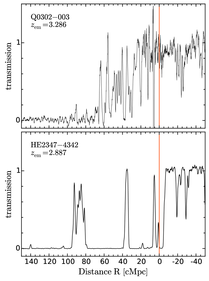
Figure 1.— UV He II Ly$\alpha$ absorption spectra ($R\sim 16,000$) of quasars Q 0302$-$003 (top; $z_{\rm em}=3.286$) and HE 2347$-$4342 (bottom; $z_{\rm em}=2.887$) as a function of comoving distance from the quasar. Both original spectra were rebinned by a factor of $3$ to yield the Nyquist sampling and then smoothed with a ‘boxcar’ kernel of width $w=11$. Red vertical lines indicate the location of the quasars.

Current constraints on the quasar lifetime are weak ($t_{\rm lt}\gtrsim 10^{4}$ yr; Martini, 2004), such that lifetimes comparable to the Salpeter time are still plausible. This limit derives from the line-of-sight H I proximity effect – the enhancement in the ionization state of H I in the quasar environment as probed by the H I Ly$\alpha$ forest. The argument is that the presence of a line-of-sight H I proximity effect in $z\sim 2-4$ quasars implies that quasars have been emitting continuously for an equilibration timescale, which corresponds to about $10^{4}$ yr in the $z\sim 2-4$ IGM. Schawinski et al. (2010) and Schawinski et al. (2015) argued for variability of several orders of magnitude in quasar luminosity on short $\sim 10^{5}\,{\rm yr}$ timescales, based on the photoionization of quasar host galaxies and light travel time arguments. However, these constraints are indirect and plausible alternative scenarios related to AGN obscuration could explain the observations without invoking short timescale quasar variability. Furthermore, the discovery of quasar powered giant Ly$\alpha$ nebulae at $z\sim 2$ (Cantalupo et al., 2014; Hennawi et al., 2015) with sizes of $\sim 500\,{\rm pkpc}$ implies quasar lifetimes of $\gtrsim 10^{6}{\rm yr}$, in conflict with the Schawinski et al. (2010) and Schawinski et al. (2015) estimates. Recently, the presence of high-equivalent width (EW${}_{{\rm Ly}\alpha}\geq 100$Å) Ly$\alpha$ emitters (LAEs) at large distances $\sim 3-20\,{\rm pMpc}$ from hyper-luminous quasars has been used to argue for quasar lifetimes in the range of $1\,{\rm Myr}\lesssim t_{\rm Q}\lesssim 30\,{\rm Myr}$, based on the presumption that such LAEs result from quasar powered Ly$\alpha$ fluoresence (Trainor & Steidel, 2013; Borisova et al., 2015). However, at such large distances $\sim 3-20\,{\rm pMpc}$ the fluorescent boost due to the quasar is far fainter than the fluxes of the LAEs in the Trainor & Steidel (2013) and Borisova et al. (2015) surveys, and hence some other physical process intrinsic to the LAE and unrelated to quasar radiation must be responsible for these sources.

There is an analogous proximity effect in the He II Ly$\alpha$ forest that, as this paper shows, is much more sensitive to the quasar lifetime than the line-of-sight H I proximity effect. The He II proximity effect has been detected at $2.7<z<3.9$ (Hogan et al., 1997; Anderson et al., 1999; Heap et al., 2000; Syphers & Shull, 2014; Zheng et al., 2015). Figure 1 shows the two well-studied examples (Shull et al., 2010; Syphers & Shull, 2014) that highlight the observed variance in He II proximity zone sizes and shapes (Zheng et al., 2015). HE 2347$-$4342 may be either young ($t_{\rm Q}<1$ Myr, Shull et al., 2010) or peculiar due to an infalling absorber (Fechner et al., 2004). Q 0302$-$003 shows a large proximity zone of $60-100$ comoving Mpc depending on the local density field (Syphers & Shull, 2014). Adopting a plausible range in the other relevant parameters (quasar luminosity, IGM He II fraction and IGM clumpiness), Syphers & Shull (2014) find that Q 0302$-$003 may have shone for $0.2-31$ Myr. The simplifying assumptions of a homogeneous IGM with a He II fraction of unity only allow for rough estimates of the quasar lifetime (Hogan et al., 1997; Anderson et al., 1999; Zheng et al., 2015).

In addition, constraints on the quasar lifetime have also been derived from the so-called transverse proximity effect, i.e. the enhancement of the UV radiation field around a foreground quasar which gives rise to increased IGM transmission in a background sightline. While several effects like anisotropic quasar emission, episodic quasar lifetimes, and overdensities around quasars make a statistical detection of the transverse proximity effect challenging (e.g. Hennawi et al., 2006; Hennawi & Prochaska, 2007; Kirkman & Tytler, 2008; Furlanetto & Lidz, 2011; Prochaska et al., 2013b), it has been detected in a few cases, either as a spike in the IGM transmission (Jakobsen et al., 2003; Gallerani et al., 2008) or as a locally harder UV radiation field in the background sightline (Worseck & Wisotzki, 2006; Worseck et al., 2007; Gonçalves et al., 2008; McQuinn & Worseck, 2014). For the handful of quasars for which such detections have been claimed, the transverse light crossing time between the foreground quasar and the background sightline provides a lower limit to the quasar lifetime of $t_{\rm Q}=10-30$ Myr.

The goal of this paper is to understand whether the properties of He II Ly$\alpha$ line-of-sight proximity zones can constrain the duration of the quasar phase. This work is motivated by the large number of He II Ly$\alpha$ forest proximity zones that have been observed over the last five years with the Cosmic Origins Spectrograph (COS) onboard the Hubble Space Telescope (HST; Shull et al., 2010, Worseck et al., 2011, Syphers et al., 2012). Another motivation is to generalize previous analyses from the restrictive assumption of $x_{\rm HeII}=1$. Even for ionized gas, He II proximity zones around $z\simeq 3$ quasars provide a much more powerful tool for constraining quasar lifetimes than H I proximity zones. In order to produce a detectable proximity zone, the quasar must shine for a time comparable to or longer than the timescale for the IGM to attain equilibrium with the enhanced photoionization rate $\Gamma$, known as the equilibration timescale $t_{\rm eq}\simeq\Gamma^{-1}$. Current measurements of the UV background in the $z\sim 3$ H I Ly$\alpha$ forest yield an H I photoionization rate $\Gamma_{\rm HI}^{\rm bkg}\simeq 10^{-12}\,{\rm s^{-1}}$ (Becker et al., 2013) implying $t_{\rm eq}\simeq 3\times 10^{4}\,{\rm yr}$. On the other hand, as we argue in § 3, current optical depth measurements at $z\sim 3$ (Worseck et al., 2011) imply a He II photoionization rate $\Gamma_{\rm HeII}^{\rm bkg}\simeq 10^{-15}\,{\rm s^{-1}}$, resulting in $t_{\rm eq}\simeq 3\times 10^{7}\,{\rm yr}$. Thus, He II proximity zones can probe quasar lifetimes three orders of magnitude larger, closer to the Salpeter timescale. Moreover, the fact that the He II background is $\sim 1000$ times lower than the H I background implies that the radius within which the quasar dominates over the background will be $\sim 30$ times larger for He II, and given these much larger zones uncertainties due to density enhancements around the quasar will be much less significant (Faucher-Giguère et al., 2008).

This paper is organized as follows. We discuss the numerical simulations we use and describe our radiative transfer algorithm in § 2. In § 3 we explore the physical conditions in the He II proximity zones of $z\simeq 3$ quasars. We introduce the idea of computing stacked spectra and study their dependence on the parameters governing quasars and the IGM in § 4. We discuss our results in § 5 and list our conclusions in § 7.

Throughout this work we assume a flat $\Lambda$CDM cosmology with Hubble constant $h=0.7$, $\Omega_{\rm m}=0.27$, $\Omega_{\rm b}=0.046$, $\sigma_{8}=0.8$ and $n_{s}=0.96$ (Larson et al., 2011), and helium mass fraction $Y_{\rm He}=0.24$. All distances are in unites of comoving Mpc, i.e., cMpc.

In order to avoid confusion, we distinguish between several different timescales that govern the duration of quasar activity. As noted above, the duty cycle $t_{\rm dc}$ refers to the total time that galaxies shine as active quasars integrated over the age of the universe. On the other hand, one of the goals of this paper is to understand the constraints that can be put on the episodic lifetime $t_{\rm episodic}$, which is the time spanned by a single episode of accretion onto the SMBH. But in the context of proximity effects in the IGM, one actually only constrains the quasar on-time, which will denote as $t_{\rm Q}$. If we imagine that time $t=0$ corresponds to the time when the quasar emitted light that is just now reaching our telescopes on Earth, then the quasar on-time is defined such that the quasar turned on at time $-t_{\rm Q}$ in the past. This timescale is, in fact, a lower limit on the quasar episodic lifetime $t_{\rm episode}$, which arises from the fact that we observe a proximity zone at $t=0$ when the quasar has been shining for time $t_{\rm Q}$, whereas this quasar episode may indeed continue, which we can only record on Earth if we could conduct observations in the future. For simplicity in the text, we will henceforth refer to the quasar on-time as the quasar lifetime denoted by $t_{\rm Q}$, but the reader should always bear in mind that this is a lower limit on the quasar episodic lifetime.

2. Numerical Model

2.1. Hydrodynamical Simulations

To study the impact of quasar radiation on the intergalactic medium we post-process the outputs of a smooth particle hydrodynamics (SPH) simulation using a one-dimensional radiative transfer algorithm. For the cosmological hydrodynamical simulation, we use the Gadget-3 code (Springel, 2005c) with $2\times 512^{3}$ particles and a box size of $25h^{-1}$ cMpc. We extract 1000 sightlines, which we will refer to as skewers, from the SPH simulation output at a snapshot corresponding to $z=3.1$. In § 5.2 we also consider skewers at a higher redshift of $z=3.9$. We identify quasars in the simulation as dark matter halos with masses $M>5\times 10^{11}M_{\odot}$, by running a friends-of-friends algorithm (Davis et al., 1985) on the dark matter particle distribution. While this mass threshold is $1$ dex lower than the halo mass inferred from quasar clustering measurements (White et al., 2012; Conroy & White, 2013), our simulation cube does not capture enough such massive halos. However, because the He II proximity effect extends many correlation lengths ($r_{0}\approx 10h^{-1}$ Mpc, White et al., 2012), the use of the less clustered halos will not make a difference at most radii we consider.

Starting from the location of the quasars, we create skewers by casting rays through the simulation volume at random angles, and traversing the box multiple times. We use the periodic boundary conditions to wrap a skewer through the box along the chosen direction. This procedure results in skewers from the quasar location through the intergalactic medium that are $318$ cMpc long, significantly larger than the length of our simulation box and the He II proximity region. Our skewers have $27,150$ pixels which corresponds to a spatial interval of ${\rm d}R=0.012$ cMpc or a velocity interval ${\rm d}v=0.893\ {\rm km\ s^{-1}}$. This is sufficient to resolve all the features in the He II Ly$\alpha$ forest.

2.2. Radiative Transfer

We extract the one-dimensional density, velocity, and temperature distributions along these skewers and use them as input to our post-processing radiative transfer algorithm, which is based on C²-Ray algorithm (Mellema et al., 2006). Because this algorithm is explicitly photon conserving, it enables great freedom in the size of the grid cells and the time step. Our one-dimensional radiative transfer algorithm is extremely fast, with one skewer calculation taking $\sim 5$ seconds on a desktop machine, allowing us to run many realizations. In this section, we describe the salient features of our radiative transfer algorithm, and we refer the reader to the original Mellema et al. (2006) paper on the C²Ray code for additional details.

We put a single source of radiation, the quasar, at the beginning of each sightline, and trace the change in the ionization state and temperature of the IGM for a finite time, $t$, as the radiation is propagated. The spectral energy distribution (SED) of the source is modeled as a power-law, such that the quasar photon production rate at any frequency $\nu\geq\nu_{\rm th}$ is

$$N_{\nu}=\frac{\alpha Q_{\rm 4Ry}}{\rm\nu_{th}}\left(\frac{\rm\nu}{\nu_{\rm th}}\right)^{-\alpha-1},$$ (1)

where $Q_{\rm 4Ry}$ is the photon production rate above the He II ionization threshold of $4\,{\rm Ry}$ or a corresponding threshold frequency $\nu_{\rm th}=1.316\times 10^{16}\ {\rm Hz}$ corresponding to this threshold. We assume a spectral index of $\alpha=1.5$, $f_{\nu}\sim\nu^{-\alpha}$, consistent with the measured values in stacked UV spectra of quasars (Telfer et al., 2002; Shull et al., 2012; Lusso et al., 2015).

The $r$-band magnitudes of He II quasars in the HST/COS archive range from $r=16.0-19.4$, with a median value of $r\simeq 18.25$. Following the procedure described in Hennawi et al. (2006), we model the quasar spectral-energy distribution (SED) using a composite quasar spectrum which has been corrected for IGM absorption (Lusso et al., 2015). By integrating the Lusso et al. (2015) composite redshifted to $z=3.1$ against the SDSS filter, we can relate the $r$-band magnitude of a quasar to the photon production rate at the H I Lyman limit $Q_{\rm 1Ry}$, which is then related to $Q_{\rm 4Ry}$ by $Q_{\rm 4Ry}=Q_{\rm 1Ry}\times 4^{-\alpha}$, assuming the same power law SED governs the quasar spectrum for frequencies blueward of $1$ Ry. This procedure implies that quasars in the range $r=16.0-19.4$ have $Q_{\rm 4Ry}=10^{56.0-57.4}$ ${\rm s}^{-1}$, with median $r\simeq 18.25$ and $Q_{\rm 4Ry}=10^{56.5}$ ${\rm s}^{-1}$.

The quasar photoinization rate in every cell is given by

$$\Gamma_{\rm QSO}=\int_{\nu_{\rm th}}^{\infty}\frac{N_{\rm\nu}e^{-\langle\tau_{\rm\nu}\rangle}}{h_{\rm P}\nu}\frac{1-e^{-\langle\delta\tau_{\rm\nu}\rangle}}{\langle n_{\rm HeII}\rangle V_{\rm cell}}d\nu,$$ (2)

where $\langle\tau_{\nu}\rangle$ is the optical depth along the skewer from the source to the current cell, $\langle\delta\tau_{\nu}\rangle$ is the optical depth inside the cell, $\langle n_{\rm HeII}\rangle$ is the average number density of He II in this cell, $V_{\rm cell}$ is the volume of the cell, and $h_{\rm p}$ is Planck’s constant. Here the angular brackets indicate time averages over the discrete time step $\delta t$.

Combining with eqn. (1), we can then rewrite eqn. (2) as

$$\Gamma_{\rm QSO}=\frac{\alpha Q_{\rm 4Ry}}{n_{\rm HeII}V_{\rm cell}\nu_{\rm th}}\int_{\nu_{\rm th}}^{\infty}\left(\frac{\nu}{\nu_{\rm th}}\right)^{-(\alpha+1)}e^{-\langle\tau_{\rm\nu}\rangle}\left(1-e^{-\langle\delta\tau_{\nu}\rangle}\right)d\nu.$$ (3)

Although this equation for the photoionization rate is an integral over frequency, in practice the code is not tracking multiple frequencies. For the power-law quasar SED that we have assumed, and He II ionizing photon absorption cross section $\sigma_{\nu}\approx\sigma_{\rm th}(\nu/\nu_{\rm th})^{-3}$, eqn. (3) has an analytic solution that depends on $\langle\tau_{\rm th}\rangle$ and $\langle\delta\tau_{\rm th}\rangle$, the time-averaged optical depth to the cell and inside the cell, respectively, evaluated at the He II ionization threshold. Thus, given the values for these optical depths evaluated at the single edge frequency, we can compute the frequency-integrated photoionization rate.

The foregoing has considered the case of a single source of radiation, namely the quasar. This scenario is likely appropriate early on in He II reionization, when each quasar photoionizes its own He III zone. However, at later times, the intergalactic medium is filled with He II ionizing photons emitted by many sources. In order to properly model the radiative transfer along our skewer, we need to account for additional ionizations caused by this intergalactic ionizing background. We approximate this background $\Gamma_{\rm HeII}^{\rm bkg}$ as being a constant in space and time, and simply add it into each pixel of our sightline to model the presence of these other sources

$$\Gamma_{\rm tot}=\Gamma_{\rm QSO}+\Gamma_{\rm HeII}^{\rm bkg}.$$ (4)

As such, this procedure does the full one-dimensional radiative transfer to compute the photoionization rate $\Gamma_{\rm QSO}$ produced by the quasar, but it would treat the background as an unattenuated and homogeneous radiation field present at every location. However, the densest regions of the IGM will be capable of self-shielding against ionizing radiation, thus giving rise to He II Lyman-limit systems (He II-LLSs). Within these systems our $1$D radiative transfer algorithm always properly attenuates the quasar photoionization rate $\Gamma_{\rm QSO}$, however, if we take the the He II ionizing background $\Gamma_{\rm HeII}^{\rm bkg}$ to be constant in every pixel along the skewers, this would be effectively treating the He II-LLSs as optically thin, thus underestimating the He II fraction in the densest regions. In order to more accurately model the attenuation of the He II background by the He II-LLSs, we implement an algorithm described in McQuinn & Switzer (2010). In Appendix B we summarize this approach and show that the effect of self-shielding of He II-LLSs to the He II background $\Gamma_{\rm HeII}^{\rm bkg}$ has a negligible effect on the structure of the He II proximity zones. We nevertheless treat the He II LLSs with this technique for all of the results described in this paper. In § 5.2 we also discuss the impact of spatial fluctuations in the He II ionizing background $\Gamma_{\rm HeII}^{\rm bkg}$ on our results (showing that the average transmission profile is largely unaffected by such fluctuations).

Having arrived at an expression for the photoionization rate in each cell, the next step is to determine the evolution of the He II fraction $x_{\rm HeII}$ in response to this time-dependent $\Gamma_{\rm tot}\left(t\right)$. The time evolution of the He II fraction is given by

$$\frac{dx_{\rm HeII}}{dt}=-\Gamma_{\rm tot}(t)\,x_{\rm HeII}+\alpha_{\rm A}n_{\rm e}\left(1-x_{\rm HeII}\right),$$ (5)

which if $n_{\rm e}$ is independent of $x_{\rm HeII}$ (which holds at the $6\%$ level) has the solution of

$$x_{\rm HeII}\left(t\right)=x_{\rm HeII,0}{\rm e}^{-\int_{0}^{t}dt^{\prime}t_{\rm eq}(t^{\prime})^{-1}}+\int_{0}^{t}dt^{\prime}\alpha_{\rm A}n_{\rm e}{\rm e}^{-\int_{0}^{t^{\prime}}dt^{\prime\prime}t_{\rm eq}(t^{\prime\prime})^{-1}}.$$ (6)

where $x_{\rm HeII,0}$ is the initial singly ionized fraction and $t_{\rm eq}$ is the equilibration timescale given by

$$t_{\rm eq}=\left(\Gamma_{\rm tot}+n_{\rm e}\alpha_{\rm A}\right)^{-1},$$ (7)

$n_{\rm e}$ is the electron density, and $\alpha_{\rm A}$ is the Case A recombination coefficient. In the limit when $\Gamma_{\rm tot}(t)$ does not change over $t$ (and also the same for $\alpha_{\rm A}n_{e}$ which is less of an approximation) eqn. (6) simplifies considerably to

$$x_{\rm HeII}\left(t\right)=x_{\rm HeII,eq}+\left(x_{\rm HeII,0}-x_{\rm HeII,eq}\right)e^{-t/t_{\rm eq}},$$ (8)

where we have defined the equilibrium He II fraction as

$$x_{\rm HeII,eq}=\alpha_{\rm A}n_{\rm e}t_{\rm eq}.$$ (9)

We discuss our treatment of He II ionizing photons produced by recombinations and the justification for adopting Case A in § 2.5 below. We have ignored collisional ionizations which contribute negligibly in proximity zones, where gas is relatively cool $\left(T\sim 10^{4}{\rm K}\right)$, and are even more highly suppressed for He II relative to H I. Given that the He II fraction starts at an initial value $x_{\rm HeII,0}$, eqn. (8) gives the He II fraction at a later time $t$, provided that $\Gamma_{\rm tot}$, $n_{\rm e}$, and $\alpha_{\rm A}$ are constant over this interval. As such, this equation is only exact for infinitesimal time intervals.

Following Mellema et al. (2006), we can compute the time averaged He II fraction inside a cell by averaging eqn. (8) over the discrete time-step $\delta t$, yielding

$$\langle x_{\rm HeII}\rangle=x_{\rm HeII,eq}+\left(x_{\rm HeII,t}-x_{\rm HeII,eq}\right)\left(1-e^{-\frac{\delta t}{t_{\rm eq}}}\right)\frac{t_{\rm eq}}{\delta t},$$ (10)

where $x_{\rm HeII,t}$ is the He II fraction at the previous timestep $t$. We then use eqn. (10) to calculate the time-averaged optical depth in the cell at the He II edge

$$\langle\delta\tau_{\rm th}\rangle=\langle x_{\rm HeII}\rangle n_{\rm He}\sigma_{\rm th}\Delta r,$$ (11)

where $\Delta r$ is the size of the cell. Likewise, the time-averaged optical depth to the cell $\langle\tau_{\rm th}\rangle$ is computed by adding, in causal order, all the $\langle\delta\tau_{\rm th}\rangle$ of the cells lying between the source and the cell under consideration. The electron density $\langle n_{\rm e}\rangle$ and number density of He II atoms $\langle n_{\rm HeII}\rangle$ are similarly computed using eqn. (10).

The iterative process that we employ to find the new ionization state in each cell (see the flow-chart in Fig 2 of Mellema et al., 2006) can be described as follows. Starting with the cell nearest the source and moving outward, we:

1. Set the mean He II fraction $\langle x_{\rm HeII}\rangle$ to that given by the previous time-step (or the initial conditions).

2. Evaluate the optical depth between the source and the cell $\langle\tau_{\rm th}\rangle$ by summing the $\delta\tau_{\rm th}$ from the previous time-step.

3. Iterate the following until convergence of the He II fraction $\langle x_{\rm HeII}\rangle$ is achieved

   • compute the time-averaged optical depth $\langle\delta\tau_{\rm th}\rangle$ within the cell (eqn. 11);

   • compute the photoionization rate $\Gamma_{\rm tot}$ (eqns. 3 and 4);

   • compute the mean electron number density based on the current mean ionization state;

   • calculate the new He II fraction $x_{\rm HeII}\left(t\right)$ at this time step (eqn. 8), as well as its time-step averaged value $\langle x_{\rm HeII}\rangle$ (eqn. 10)

   • check for convergence

4. Once convergence is reached, advance to the next cell.

Following this procedure for every time-step, we thus integrate the time-evolution over time interval $t_{\rm Q}$, which denotes the quasar lifetime, yielding the He II fraction $x_{\rm HeII}$ at each location in space in the proximity zone.

2.3. Heating and Cooling of the Gas

We assume that the excess from photoionization of helium heats the surrounding gas. In reality, instead of heating, the electron produced during the photoionization, can become a source of secondary (collisional) ionization, but they are unimportant for the highly ionized IGM, which will clearly be the case for He II proximity zones. The amount of heat injected per time interval is given by (Abel & Haehnelt, 1999)

$$\frac{{\rm d}T}{{\rm d}t}\approx\frac{2Y_{\rm He}}{3k_{\rm B}(8-5Y_{\rm He})}\langle E\rangle\frac{{\rm d}x_{\rm HeII}}{{\rm d}t}$$ (12)

where ${\rm d}x_{\rm HeII}/{\rm d}t$ is the change in the He II fraction over the time step and $\langle E\rangle$ is the average excess energy of a photon above He II ionization threshold, which is given by

$$\langle E\rangle=\left[\frac{\int_{\nu_{\rm th}}^{\infty}N_{\nu}\sigma_{\nu}e^{-\langle\tau_{\rm\nu}\rangle}\left(1-e^{-\langle\delta\tau_{\nu}\rangle}\right)\left(h_{\rm P}\nu-h_{\rm P}\nu_{\rm th}\right){\rm d}\nu}{\int_{\nu_{\rm th}}^{\infty}N_{\nu}\sigma_{\nu}e^{-\langle\tau_{\rm\nu}\rangle}\left(1-e^{-\langle\delta\tau_{\nu}\rangle}\right){\rm d}\nu}\right]$$ (13)

For a power law SED, this frequency integral can be solved analytically, and yields a function that depends on the optical depth between the source and the current cell $\langle\tau_{\nu}\rangle$ and optical depth of the cell $\langle\delta\tau_{\nu}\rangle$. This function is evaluated at each time step and the resulting change in the temperature added to each cell. We ignore the heating caused by the He II ionizing background $\Gamma_{\rm HeII}^{\rm bkg}$, since this is accounted for via the photoionization heating in the hydrodynamical simulations (and it does not depend on the normalization of the photoionizing background, which we freely adjust). We also do not include cooling in our simulations because the gas cooling time at mean density is comparable to the Hubble time which is much longer than the expected lifetime of the quasar (i.e., $t_{\rm cool}\gg t_{\rm Q}$) and thus can be safely ignored.

2.4. Finite Speed of Light

Our code works in the infinite speed of light limit, similar to other one-dimensional radiative transfer codes which attempt to model observations along the line-of-sight (White et al., 2003; Shapiro et al., 2006; Bolton & Haehnelt, 2007a; Lidz et al., 2007; Davies et al., 2014). Thus, the results do not depend on the speed of light, which may seem problematic because the light travel times across the proximity region can be tens of Myr. However, in Appendix A, we show that because absorption observations also occur along the light-cone, the infinite speed of light assumption exactly describes the ionization state of the gas probed by line-of-sight observations.

2.5. Recombinations

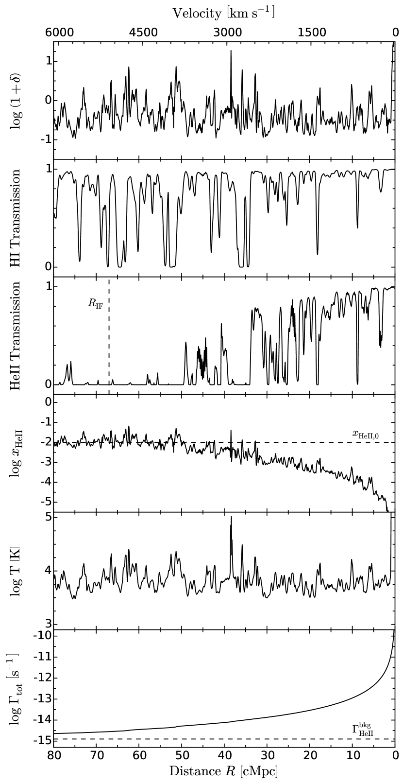
Figure 2.— Example sightline at $z=3.1$ from our radiative transfer code assuming a quasar has been on for $t_{\rm Q}=10^{7}$yr at a photon production rate $Q_{\rm 4Ry}=10^{56.1}\ {\rm s^{-1}}$ with He II ionizing background $\Gamma_{\rm HeII}^{\rm bkg}=10^{-14.9}{\rm s^{-1}}$. The lower x-axis indicates distance $R$ from the quasar in units of comoving Mpc, whereas the upper x-axis is the corresponding velocity in units of ${\rm km\ s^{-1}}$. Panels show (from top to bottom): the overdensity, transmitted flux in hydrogen, transmitted flux in helium, the He II fraction $x_{\rm HeII}$, temperature $T$, photoionization rate $\Gamma_{\rm tot}$. The vertical dashed line in the panel with He II transmission shows the extent of the quasar ionization front (see § 3.2 for the description). We indicate the initial He II fraction before the quasar is on by the dashed line in the panel with $x_{\rm HeII}$ evolution. The dashed line in the bottom panel indicates the value of the He II ionizing background $\Gamma_{\rm HeII}^{\rm bkg}$.

We use the Case A recombination coefficient throughout the paper. Quasar proximity zones represent highly ionized media which typically have $x_{\rm HeII}\lesssim 10^{-2}$, making most cells optically thin to ionizing photons produced by recombinations directly to the ground state. This recombination radiation is an additional source of ionizations, but we do not include it in our computations. We show in Appendix C that neglecting secondary ionizations from recombination radiation is justified as it is negligible in comparison to the quasar radiation.

2.6. Radiative Transfer Outputs

We calculate He II spectra along each of the sightlines taken from the SPH simulations following the procedure described in Theuns et al. (1998), which we outline in Appendix D. Figure 2 shows various physical properties along an example line-of-sight. The quasar is located on the right side of the plot at $R=0$. These physical properties are drawn from a model that has the quasar lifetime set to $t_{\rm Q}=10$ Myr, the photon production rate $Q_{\rm 4Ry}=10^{56.1}\ {\rm s^{-1}}$, and the He II ionizing background $\Gamma_{\rm HeII}^{\rm bkg}=10^{-14.9}{\rm s^{-1}}$, which is our preferred value following the discussion in § 3.1.

The uppermost panel of Figure 2 shows the gas density along the skewer in units of the cosmic mean density, illustrating the level of density fluctuations present in the $z=3.1$ IGM. The second panel shows the H I transmitted flux, which exhibits the familiar absorption signatures characteristic of the Ly$\alpha$ forest. A weak H I proximity effect (Carswell et al., 1982; Bajtlik et al., 1988) is noticeable by eye near the quasar for $R\lesssim 20$ cMpc. This weak H I proximity effect is expected: given the high value of the H I ionizing background, the region where the quasar radiation dominates over the background is relatively small. Furthermore, the low H I Ly$\alpha$ optical depth at $z=3.1$ reduces the contrast between the proximity zone and regions far from the quasar. On the contrary, the He II transmission clearly indicates the large and prominent ($\simeq 50$ cMpc) He II proximity zone around the quasar. At larger distances $R>50$ cMpc the transmission drops to nearly zero, giving rise to long troughs of Gunn-Peterson (GP; Gunn & Peterson, 1965) absorption, as is commonly observed in the He II transmission spectra of quasars observed with HST (Worseck et al., 2011; Syphers & Shull, 2014). This GP absorption results from the large He II optical depth in the ambient IGM, which is in turn set by our choice of $\Gamma_{\rm HeII}^{\rm bkg}=10^{-14.9}{\rm s^{-1}}$. The He II transmission follows the radial trend set by the He II fraction $x_{\rm HeII}$. As expected, close to the quasar $R\lesssim 20$ cMpc, helium is highly ionized ($x_{\rm HeII}<10^{-3}$) by the intense quasar radiation. At larger radii the quasar photoionization rate weakens, dropping approximately as $R^{-2}$, as indicated in the bottom panel. Eventually, at large distances $R\gtrsim 70$ cMpc the quasar radiation no longer dominates over the the background $\Gamma_{\rm HeII}^{\rm bkg}$, and $x_{\rm HeII}$ gradually asymptotes to a value $x_{\rm HeII,0}\simeq 10^{-2}$, set by the chosen He II ionizing background.

3. Physical Conditions in the Proximity Zone

The transmitted flux in the proximity zone results from an interplay between different parameters. In order to constrain the quasar lifetime, $t_{\rm Q}$, independently from other parameters, such as the He II ionizing background $\Gamma_{\rm HeII}^{\rm bkg}$ or the rate at which He II ionizing photons are emitted by the quasar $Q_{\rm 4Ry}$, we need to understand the impact of each one of them on the structure of the proximity zone. We begin first by considering the constraints on $\Gamma_{\rm HeII}^{\rm bkg}$ from observational data.

3.1. Constraints on the He II ionizing background $\Gamma_{\rm HeII}^{\rm bkg}$

In order to model the He II proximity regions, we need to make some assumptions about the background radiation field in the IGM. At $z\gtrsim 2.8$ this background may not be spatially uniform, as it has been argued that He II reionization is occurring (McQuinn, 2009b; Shull et al., 2010). He II reionization is thought to be driven by quasars turning on and emitting the hard photons required to doubly ionize helium (Madau & Meiksin, 1994; Miralda-Escudé et al., 2000; McQuinn et al., 2009a; Haardt & Madau, 2012; Compostella et al., 2013). At $z=3.1$, redshifts characteristic of much of the COS data, the IGM is still likely to consist of mostly reionized He III regions, but there may be some quasars that turn on in He II regions. The latter case should become increasingly more likely with increasing redshift. In this paper we model the full range of possibilities, but let us first get a sense for what currently available data implies about typical regions of the IGM.

Recent measurements of the He II effective optical depth $\tau_{\rm eff}$ from Worseck et al. (2014) & Worseck et al. in prep, albeit with large scatter, imply $\langle\tau_{\rm eff}^{\rm HeII}\rangle\simeq 4-5$ on scales $\Delta z=0.04$ ($\Delta R\simeq 40$ cMpc) at $z\sim 3.1$ (see the upper panel of Figure 3). We use our $1$D radiative transfer algorithm to try to understand how these observational results constrain the He II ionizing background $\Gamma_{\rm HeII}^{\rm bkg}$. Similarly to Worseck et al. (2014), we exclude the proximity zone from our calculations by turning the quasar off. The resulting transmission through the IGM is solely due to the He II background $\Gamma_{\rm HeII}^{\rm bkg}$. We then vary $\Gamma_{\rm HeII}^{\rm bkg}$, and calculate the effective optical depth defined by $\tau_{\rm eff}\equiv-\ln\langle F\rangle$, where we take the average of the simulated transmission $F$ in $5$ regions along $100$ skewers, each region with size $\Delta z=0.04$ equal to the size of the bin in the observations. We also calculate the average value of the He II fraction $\langle x_{\rm HeII}\rangle$ in the same bins.

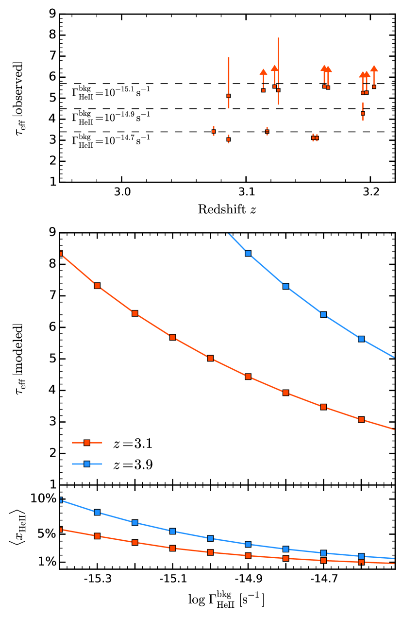
Figure 3.— Results of the radiative transfer simulations with just a uniform He II ionizing background and no quasar source. The red curve corresponds to the calculations performed at redshift $z=3.1$, while the blue curve is for $z=3.9$. Top panel: the observed distribution of the He II effective optical depth at $z=3.0-3.2$ from Worseck et al. (2014) & Worseck et al. in prep. The dashed curves show the mean effective optical depths on the same spatial scale as data ($\Delta z=0.04$) corresponding to the indicated $\Gamma_{\rm HeII}^{\rm bkg}$ value in the $1$D radiative transfer simulations. Middle panel: He II effective optical depth $\tau_{\rm eff}$ as a function of the He II ionizing background field $\Gamma_{\rm HeII}^{\rm bkg}$ from our $1$D radiative transfer algorithm. Bottom panel: He II fraction $x_{\rm HeII}$ as a function of He II background $\Gamma_{\rm HeII}^{\rm bkg}$.

The results are shown in Figure 3. The solid red line in the middle panel shows the values of our modeled He II effective optical depth as a function of the He II ionizing background $\Gamma_{\rm HeII}^{\rm bkg}$. The corresponding He II fraction $\langle x_{\rm HeII}\rangle$ is shown in the bottom panel of Figure 3. We find that the effective optical depth $\tau_{\rm eff}\simeq 4-5$ implies a characteristic He II ionizing background of $\Gamma_{\rm HeII}^{\rm bkg}\simeq 10^{-14.9}{\rm s}^{-1}$, which will refer to henceforth as our fiducial value for $z=3.1$. This He II background corresponds to an average He II fraction $\langle x_{\rm HeII}\rangle\simeq 0.02$. While uniformity is likely not a good assumption during He II reionization, which makes the above number highly approximate (and probably an underestimate for $x_{\rm HeII}$), it is a good assumption thereafter, i.e. $z\simeq 2.5$, where fluctuations of He II ionizing background are on the order of unity (McQuinn & Worseck, 2014).

We also preformed the same set of calculations at higher redshift of $z=3.9$ and plot the results as blue curves in Figure 3. Note, that at higher redshifts the gas in the intergalactic medium is becoming more dense, and the steep redshift dependence of the GP optical depth $\tau_{\rm GP}\propto(1+z)^{3/2}$ gives rise to significantly higher optical depths at $z=3.9$. Thus at these high redshifts even He II fractions of $x_{\rm HeII}\sim 0.01$ give rise to large effective optical depths $\tau_{\rm eff}\gtrsim 5$. While we mostly consider $z=3.1$, § 5.2 considers $z\simeq 3.9$.

3.2. Time Evolution of the Ionized Fraction

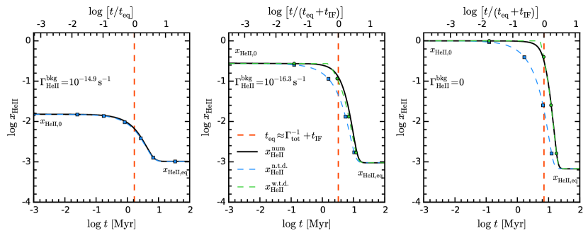
Figure 4.— Time evolution of the He II fraction, $x_{\rm HeII}\left(t,R\right)$, at a single location in the proximity zone at $R=25$ cMpc, produced from our radiative transfer solution (solid black curve), compared to the analytical expression given by eqn. (16) (dashed blue curve with square markers). The left panel shows the results for a model with $\Gamma_{\rm HeII}^{\rm bkg}=10^{-14.9}{\rm s^{-1}}$ ($x_{\rm HeII,0}\simeq 0.02$). The middle panel is the same, but for $\Gamma_{\rm HeII}^{\rm bkg}=10^{-16.3}{\rm s^{-1}}$ ($x_{\rm HeII,0}\simeq 0.3$). The zero background model $\Gamma_{\rm HeII}^{\rm bkg}=0$ (i.e., $x_{\rm HeII,0}=1$) is shown in the right panel. The dashed green curves correspond to the corrected analytical solution given by eqn. (19). The He II fraction $x_{\rm HeII,eq}$ and the equilibration time $t_{\rm eq}$ (red dashed vertical line in all panels) are evaluated using the quasar photoionization rate for a fully equilibrated IGM in the analytic expression.

Consider the case of a quasar emitting radiation for time $t_{\rm Q}$ into a homogeneous IGM with He II fraction $x_{\rm HeII}$. The time evolution of the He III ionization front is governed by the equation (Haiman & Cen, 2001; Bolton & Haehnelt, 2007a)

$$\frac{dR_{\rm IF}}{dt}=\frac{Q_{\rm 4Ry}-\frac{4}{3}R_{\rm IF}^{3}\alpha_{\rm HeIII}n_{\rm He}^{2}}{4\pi R_{\rm IF}^{2}x_{\rm HeII}n_{\rm He}},$$ (14)

which has the solution

$$R_{\rm IF}=R_{S}\left[1-{\rm exp}\left(-\frac{t_{\rm Q}}{x_{\rm HeII}t_{\rm rec}}\right)\right]^{1/3},$$ (15)

where $t_{\rm rec}=1/n_{\rm e}\alpha_{\rm A}$ is the recombination timescale and $R_{\rm S}$ is the classical Strömgren radius $R_{\rm S}=\left(\frac{3Q_{\rm 4Ry}}{4\pi\alpha_{\rm A}n_{\rm HeIII}n_{\rm e}}\right)^{1/3}$, which is the radius of the sphere around a source of radiation, within which ionizations are exactly balanced by recombinations.

Previous observational studies of the H I Ly$\alpha$ proximity zones around $z\simeq 6$ quasars have primarily focused on measuring proximity zone sizes (Cen & Haiman, 2000; Madau & Rees, 2000; Mesinger & Haiman, 2004; Fan et al., 2006; Carilli et al., 2010), guided by the faulty intuition that, for assuming a highly neutral IGM $x_{\rm HI}\sim 1$, the location where the transmission profile goes to zero can be identified with the location of the ionization front $R_{\rm IF}$ in eqn. (15). However, the transmission profile for a H II region expanding into a significantly neutral IGM can be difficult to distinguish from that of a “classical” proximity zone embedded in an already highly ionized IGM (Bolton & Haehnelt, 2007b; Maselli et al., 2007; Lidz et al., 2007). This degenerate situation arises, because even very small residual neutral fractions in the proximity zone $x_{\rm HI}\gtrsim 10^{-5}$ are sufficient to saturate H I Ly$\alpha$, which may occur well before the location of the ionization front is reached (Bolton & Haehnelt, 2007a). Thus naively identifying the size of the proximity zone with the location of the ionization front $R_{\rm IF}$, can lead to erroneous conclusions about the parameters governing eqn. (15), e.g. the quasar lifetime and the ionization state of the IGM.

A similar degeneracy also exists for He II proximity zones, which is exemplified in Figure 2 where the He II transmission saturates at $R\simeq 50$  cMpc, whereas the ionization front is located much further from the quasar $R_{\rm IF}\simeq 67$ cMpc (dashed vertical line). However, all previous work analyzing the structure of He II proximity zones has been based on the assumption that the edge of the observed proximity zone can be identified with $R_{\rm IF}$ (Hogan et al., 1997; Anderson et al., 1999; Syphers & Shull, 2014; Zheng et al., 2015). In addition, the majority of studies have assumed that helium is completely singly ionized $x_{\rm HeII}=1$ for quasars at $3.2<z<3.5$ (Hogan et al., 1997; Anderson et al., 1999; Zheng et al., 2015), whereas our discussion in the previous section (see Figure 3) indicates that at $z=3.1$ observations of the effective optical depth suggest that $\Gamma_{\rm HeII}^{\rm bkg}=10^{-14.9}{\rm s^{-1}}$ implying $x_{\rm HeII}\simeq 0.01$ (although the average $x_{\rm HeII}$ could be much larger if some regions are predominantly He II at $z>2.8$, Compostella et al. 2013; Worseck et al. 2014). Hence, in many regions one is actually in the classical proximity zone regime, where radiation from the quasar increases the ionization level of nearby material which was already highly ionized to begin with and the location of the ionizaton front is irrelevant. Furthermore, as we describe below, the background level determines the equilibration timescale $t_{\rm eq}\approx 1/\Gamma_{\rm HeII}^{\rm bkg}$ (see eqn. 7), which is the characteristic time on which the He II ionization state of IGM gas responds to the changes in the radiation field. For our fiducial value of the background $\Gamma_{\rm HeII}^{\rm bkg}=10^{-14.9}{\rm s^{-1}}$, $t_{\rm eq}\simeq 2.5\times 10^{7}\,{\rm yr}$ is comparable to the Salpeter time. This suggests that the approach of $x_{\rm HeII}$ to equilibrium is the most important physical effect in He II proximity zones, and in what follows we introduce a simple analytical equation for understanding this time evolution.

The full solution to the time evolution of $x_{\rm HeII}$ is given by eqn. (6), which involves a nontrivial integral because $\Gamma_{\rm tot}$, $n_{\rm e}$ and $\alpha_{\rm A}$ are all functions of time. Indeed, this is exactly the equation that is solved at every grid cell in our $1$D radiative transfer calculation, by integrating over infinitesimal timesteps (see eqn. 8). However, in the limit of a highly ionized IGM $x_{\rm HI}\ll 1$, $n_{\rm e}\propto(1+z)^{3}$ which is approximately constant over the quasar lifetimes we consider. Furthermore, as we will demonstrate later, the low singly ionized fraction $x_{\rm HeII}\ll 1$ implies that the attenuation is small in most of the proximity zone and, hence, the photoionization rate $\Gamma_{\rm tot}$ is also approximately constant in time. Similarly, $\alpha_{\rm A}$ varies only weakly with temperature (i.e., $\propto T^{-0.7}$), and given that the temperature will also not vary significantly with time if the HeII already has been reionized, $\alpha_{\rm A}$ can also be approximated as constant. In this regime where $\Gamma_{\rm tot}$, $n_{\rm e}$ and $\alpha_{\rm A}$ are constant in time, eqn. (8) reduces to the simpler expression evaluated at $t=t_{\rm Q}$, the quasar lifetime:

$$x_{\rm HeII}\left(t_{\rm Q}\right)=x_{\rm HeII,eq}+\left(x_{\rm HeII,0}-x_{\rm HeII,eq}\right)e^{-t_{\rm Q}/t_{\rm eq}},$$ (16)

Given that the recombination timescale $t_{\rm rec}\equiv 1/\alpha_{\rm A}n_{\rm e}\simeq 10^{9}\,{\rm yr}$ is very long compared to the longest ionization timescales $1/\Gamma^{\rm bkg}_{\rm HeiI}$, we can write $t_{\rm eq}\approx 1/\Gamma_{\rm tot}$, $x_{\rm HeII,0}\approx\alpha_{\rm A}n_{\rm e}/\Gamma^{\rm bkg}_{\rm HeII}$, and $x_{\rm HeII,eq}\approx\alpha_{\rm A}n_{\rm e}t_{\rm eq}$.

In the left panel of Figure 4, the solid black curve shows the time evolution of $x_{\rm HeII}\left(t,R\right)$ at a single location in the proximity zone $R=25$ cMpc, produced from our radiative transfer solution for the quasar photon production rate $Q_{\rm 4Ry}=10^{56.1}{\rm s^{-1}}$ and finite background case $\Gamma_{\rm HeII}^{\rm bkg}=10^{-14.9}{\rm s^{-1}}$ corresponding to an initial He II fraction $x_{\rm HeII,0}=0.02$. The dashed blue curve is the analytical solution eqn. (16). where $x_{\rm HeII,eq}$ and $t_{\rm eq}$ have been evaluated from the code outputs, using the total photoionization rate $\Gamma_{\rm tot}$ for a fully equilibrated IGM. In other words, we evaluate $\Gamma_{\rm tot}(t=\infty)=\Gamma_{\rm QSO}(t=\infty)+\Gamma_{\rm HeII}^{\rm bkg}$ where $t=\infty$ is taken to be our last output at $t=100\,{\rm Myr}$. It is clear that for the case $\Gamma_{\rm HeII}^{\rm bkg}=10^{-14.9}{\rm s^{-1}}$ and thus an initially highly ionized IGM $x_{\rm HeII}\simeq 10^{-2}$, eqn. (16) provides an excellent match to the result of the full radiative transfer calculation.

Due to the patchy and inhomogeneous nature of He II reionization some regions on the IGM might, however, have a very high He II fraction. Therefore, it is important to check if our analytical approximation also holds in this case. The middle and right panels of Figure 4 show the time evolution of the He II fraction at the same location and value of $Q_{\rm 4Ry}$, but now for $\Gamma_{\rm HeII}^{\rm bkg}=10^{-16.3}{\rm s^{-1}}$ and $\Gamma_{\rm HeII}^{\rm bkg}=0$, which correspond to $x_{\rm HeII,0}\simeq 0.3$ and $x_{\rm HeII,0}=1$ respectively. The analytical approximation (blue squares and curve) clearly fails to reproduce the time evolution. Specifically, it predicts too rapid a response to the quasar ionization relative to the true evolution, and this discrepancy is largest for $\Gamma_{\rm HeII}^{\rm bkg}=0$ where the true evolution to equilibrium is delayed by $\sim 5.5$ Myr.

Recall that, because we observe on the light cone, the speed of light is effectively infinite in our code. Thus, at the location $R=25$ cMpc we expect no delay in the response of the proximity zone to the quasar radiation caused by finite light travel time effects. For the $x_{\rm HeII,0}\simeq 0.02$ ($\Gamma_{\rm HeII}^{\rm bkg}=10^{-14.9}{\rm s^{-1}}$) case the ionization front travels at nearly the speed of light and, because we observe on the light cone, there is thus no noticeable delay between the evolution of the He II fraction and eqn. (16). However, if the ionization front does not travel at the speed of light, which will be the case for the lower backgrounds $\Gamma_{\rm HeII}^{\rm bkg}=10^{-16.3}{\rm s^{-1}}$ and $\Gamma_{\rm HeII}^{\rm bkg}=0$ and correspondingly higher He II fractions ($x_{\rm HeII,0}\simeq 0.3$ and $x_{\rm HeII,0}=1$), then the time that it takes the ionization front to propagate to the location $R=25$ cMpc is no longer negligible relative to the equilibration timescale, and the response of the He II fraction will be delayed.

We can estimate this time delay by noting that the location of the ionization front (see eqn. 15) is given by

$$R_{\rm IF}\approx\left[\frac{3Q_{\rm 4Ry}t_{\rm IF}}{4\pi n_{\rm He}x_{\rm HeII}}\right]^{1/3},$$ (17)

assuming that $t_{\rm Q}\ll x_{\rm HeII}t_{\rm rec}=(x_{\rm HeII}/1.0)1.16\times 10^{9}\,{\rm yr}$, valid for $x_{\rm HeII}\sim 0.3-1.0$ and the quasar lifetimes we consider. In this regime the ionization front is simply the radius of the ionized volume around the quasar. Inverting this equation, we obtain that at a location $R$, the time delay between the quasar turning on and the arrival of the first ionizing photons is

$$t_{\rm IF}\left(R\right)=6.7\ \left(\frac{x_{\rm HeII}}{1.0}\right)\left(\frac{{Q_{\rm 4Ry}}}{10^{56}\ {\rm s^{-1}}}\right)^{-1}\left(\frac{R}{25\ {\rm cMpc}}\right)^{3}{\rm Myr}$$ (18)

For $R=25$ cMpc this delay is very nearly the delay seen in the middle and right panels of Figure 4, suggesting a simple physical interpretation for the behavior of the He II fraction in the proximity zone for the $\Gamma_{\rm HeII}^{\rm bkg}=10^{-16.3}{\rm s^{-1}}$ and $\Gamma_{\rm HeII}^{\rm bkg}=0$ cases. Namely, eqn. (16) still describes the equilibration of the He II fraction, but it must be modified to account for the delay in the arrival of the ionization front, only after which equilibration begins to occur. We thus write

$$x_{\rm HeII}\left(t_{Q},r\right)=x_{\rm HeII,eq}+\left(1-x_{\rm HeII,eq}\right){\rm e}^{\frac{-\left(t_{\rm Q}-t_{\rm IF}\right)}{t_{\rm eq}}}$$ (19)

The green curves in the middle and right panels of Figure 4 illustrate that the simple equilibration time picture, but now modified to account for a delay in the arrival of the ionization front, provides a good description of the time evolution of $x_{\rm HeII}$ in the proximity zone for $\Gamma_{\rm HeII}^{\rm bkg}=10^{-16.3}{\rm s^{-1}}$ and $\Gamma_{\rm HeII}^{\rm bkg}=0$ cases.

To summarize, we have shown that the He II fraction in quasar proximity zones is governed by a simple analytical equation (eqn. 16), which describes the exponential time evolution from an initial pre-quasar ionization state $x_{\rm HeII,0}$ to an equilibrium value $x_{\rm HeII,eq}$. The enhanced photoionization rate near the quasar $\Gamma_{\rm tot}$ sets both the timescale of the exponential evolution $t_{\rm eq}=1/\Gamma_{\rm tot}$, and the equilibrium value attained $x_{\rm HeII,eq}\approx\alpha_{\rm A}n_{\rm e}t_{\rm eq}$. For very high He II fractions $x_{\rm HeII,0}\simeq 1$, this exponential equilibration is delayed by the time it takes the sub-luminal ionization front to arrive to a given location.

3.3. Degeneracy between Quasar Lifetime $t_{\rm Q}$ and He II Ionizing Background $\Gamma_{\rm HeII}^{\rm bkg}$

Previous work on H I proximity zones at $z\sim 6$ have pointed out that the quasar lifetime and ionization state of the IGM (or equivalently the ionizing background) are degenerate in determining the location of the ionization front $R_{\rm IF}$ (Bolton & Haehnelt, 2007a, b; Lidz et al., 2007; Bolton et al., 2012), which is readily apparent from the exponent in eqn. (15). Although, many studies simply assume a fixed value for the quasar lifetime of $t_{Q}=10^{7}\,{\rm yr}$ when making inferences about the ionization state of the IGM (but see Bolton et al., 2012, for a more careful treatment). This degeneracy between lifetime and ionizing background is complicated by the fact that, at $z\sim 6$ only lower limits on the hydrogen neutral fraction $x_{\rm HI}$ (upper limits on the background photoionization rate $\Gamma_{\rm HI}^{\rm bkg}$) can be obtained from lower limits on the GP absorption optical depth. The situation is further exacerbated if there are significant spatial fluctuations in the background caused by foreground galaxies that may have ‘pre-ionized’ the IGM (Lidz et al., 2007; Bolton & Haehnelt, 2007b; Wyithe et al., 2008).

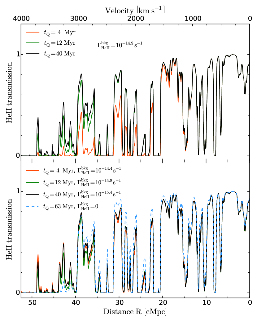
Figure 5.— Illustration of the partial degeneracy between the He II ionizing background and the quasar lifetime for the specified values of $\Gamma_{\rm HeII}^{\rm bkg}$ and $t_{\rm Q}$. The upper panel shows three models with $t_{\rm Q}=4$ Myr (red), $t_{\rm Q}=12$ Myr (green) and $t_{\rm Q}=40$ Myr (black) with He II background fixed to our fiducial value $\Gamma_{\rm HeII}^{\rm bkg}=10^{-14.9}{\rm s^{-1}}$. The bottom panel shows four models with the same values of quasar lifetime as before, but with different He II backgrounds. The red curve corresponds to $t_{\rm Q}=4$ Myr and $\Gamma_{\rm HeII}^{\rm bkg}=10^{-14.4}{\rm s^{-1}}$, whereas the solid black curve corresponds to $t_{\rm Q}=40$ Myr and $\Gamma_{\rm HeII}^{\rm bkg}=10^{-15.4}{\rm s^{-1}}$. The model with $t_{\rm Q}=12$ Myr and $\Gamma_{\rm HeII}^{\rm bkg}=10^{-14.9}{\rm s^{-1}}$ is shown by the green curve, and the dashed blue curve shows a $\Gamma_{\rm HeII}^{\rm bkg}=0$ model with $t_{\rm Q}=63$ Myr. The photon production rate is $Q_{\rm 4Ryd}=10^{56.1}{\rm s^{-1}}$ for all models.

An analogous degeneracy exists between $t_{\rm Q}$ and $x_{\rm HeII}$ for He II proximity zones, as we illustrate in Figure 5. The upper panel shows three example transmission spectra for the same skewer and value of He II background, but different values of quasar lifetime, which are clearly distinguishable. The situation changes if we also allow the He II background to vary, which is shown in the bottom panel of Figure 5 where transmission spectra are plotted for the same skewer, but several distinct combinations of lifetime and background. The nearly identical resulting spectra indicate that the same degeneracy exists at $z\simeq 3.1$ between the quasar lifetime $t_{\rm Q}$ and the value of the He II ionizing background $\Gamma_{\rm HeII}^{\rm bkg}$. In what follows, we discuss this degeneracy in detail, aided by our analytical model for the time evolution of the He II fraction from the previous section.

We can understand this degeneracy by rearranging eqn. (16)

$$x_{\rm HeII}\left(t_{\rm Q},R\right)=x_{\rm HeII,eq}\left[1+\frac{\Gamma_{\rm QSO}}{\Gamma_{\rm HeII}^{\rm bkg}}{\rm e^{-\frac{t_{\rm Q}}{t_{\rm eq}\left(R\right)}}}\right]$$ (20)

where for simplicity we have focused on the finite background case where the ionization front time delay can be ignored. There are two regimes that are relevant to this degeneracy. First, very near the quasar the attenuation of $\Gamma_{\rm QSO}$ is negligible, implying that $t_{\rm eq}\propto\Gamma_{\rm QSO}^{-1}\propto R^{2}$ and given by

$$t_{\rm eq}=0.08\,\left(\frac{{Q_{\rm 4Ry}}}{10^{56}\ {\rm s^{-1}}}\right)^{-1}\left(\frac{R}{5\,{\rm cMpc}}\right)^{2}\,{\rm Myr}.$$ (21)

At small distances ($R\lesssim 15$ cMpc in Fig. 5) in the highly ionized ‘core’ of the proximity zone, $t_{\rm eq}\ll t_{\rm Q}$ for the quasar lifetimes we consider, and eqn. (20) indicates that the proximity zone structure depends only on the luminosity of the quasar, which determines $x_{\rm HeII,eq}\approx\alpha_{\rm A}n_{\rm e}/\Gamma_{\rm QSO}$, but there is no sensitivity to either $t_{\rm Q}$ or $\Gamma_{\rm HeII}^{\rm bkg}$.

Second, at larger distances the equilibration time grows as $t_{\rm eq}\propto R^{2}$ and will eventually be comparable to the quasar lifetime. We define the equilbration distance $R_{\rm eq}$ to be the location where $t_{\rm eq}(R_{\rm eq})\equiv t_{\rm Q}$, which gives

$$R_{\rm eq}=17\,\left(\frac{Q_{\rm 4Ry}}{10^{56}\ {\rm s^{-1}}}\right)^{1/2}\left(\frac{t_{\rm Q}}{1\,{\rm Myr}}\right)^{1/2}\,{\rm cMpc},$$ (22)

where for simplicity we neglect the impact of attenuation of $\Gamma_{\rm QSO}$. At distances comparable to the equilibration distance $R\sim R_{\rm eq}$, eqn. (20) indicates that the He II fraction will be sensitive to $t_{\rm Q}$. Note that at $R\sim R_{\rm eq}$ the quasar still dominates over the background $\Gamma_{\rm QSO}\gg\Gamma_{\rm HeII}^{\rm bkg}$, such that $x_{\rm HeII,eq}$ is still independent of $\Gamma_{\rm HeII}^{\rm bkg}$. One then sees from eqn. (20) that for any change in quasar lifetime $t_{\rm Q}$ one can always make a corresponding change to the value of $\Gamma_{\rm HeII}^{\rm bkg}$ to yield the same value of $x_{\rm HeII}$. But note that this degeneracy holds only at a single radius $R$, because $t_{\rm eq}\left(R\right)$ is a function of $R$, whereas our $\Gamma_{\rm HeII}^{\rm bkg}$ is assumed to be spatially constant. Therefore, there is no way to choose a constant $\Gamma_{\rm HeII}^{\rm bkg}$ such that the $x_{\rm HeII}\left(t_{\rm Q},R\right)$ matches different values of $t_{\rm Q}$ at all $R$. In reality, $\Gamma_{\rm HeII}^{\rm bkg}$ will fluctuate spatially, but it will not have the required dependence on $R$ to counteract the lifetime dependence.

Similar arguments also apply when $\Gamma_{\rm HeII}^{\rm bkg}=0$, and the $x_{\rm HeII}(t,R)$ evolution is governed by eqn. (19). In this case, the time evolution depends only on the quasar lifetime $t_{\rm Q}$ and the ionizing photon production rate of the quasar $Q_{\rm 4Ry}$. Very close to the quasar ($R\lesssim 15$ cMpc), there is no sensitivity to quasar lifetime provided that $t_{\rm Q}-t_{\rm IF}(R)\gg t_{\rm eq}$, which is the case for the long quasar lifetime model $t_{\rm Q}=63\,$ Myr shown in Figure 5 with $\Gamma_{\rm HeII}^{\rm bkg}=0$ (dashed blue curve), which is indistinguishable from the finite background models at small radii. Although note that for much shorter quasar lifetimes $t_{\rm Q}\sim t_{\rm IF}\left(R\right)$ comparable to the ionization front travel time, eqn. (19) indicates one may retain sensitivity to the quasar lifetime even in the core of the zone. At larger distances $R\gtrsim 15$ Mpc where $t_{\rm Q}-t_{\rm IF}\left(R\right)\sim t_{\rm eq}$, the $\Gamma_{\rm HeII}^{\rm bkg}=0$ case becomes sensitive to quasar lifetime according to eqn. (19), but Figure 5 still indicates that the transmission profile is remarkably similar to the finite background case. In principle $Q_{\rm 4Ry}$ could be varied to produce a curve that appears even more degenerate, but we do not explore that here (but see the discussion in § 5.2).

Finally, an obvious difference between the $\Gamma_{\rm HeII}^{\rm bkg}=0$ and finite background case is of course the transmission level far from the quasar, which is zero for $\Gamma_{\rm HeII}^{\rm bkg}=0$, but corresponds to a finite value of $\tau_{\rm eff}$ for $\Gamma_{\rm HeII}^{\rm bkg}\neq 0$ (see Figure 3). At low redshifts $z\simeq 3$ where the effective optical depth can be measured, this provides an independent constraint on $\Gamma_{\rm HeII}^{\rm bkg}$ which rules out a $\Gamma_{\rm HeII}^{\rm bkg}=0$ model. As discussed in § 3.1, the enhanced sensitivity of $\tau_{\rm eff}$ measurements to the He II background level for He II GP absorption at $z\sim 3$, as compared to H I GP absorption at $z\sim 6-7$ (where only upper limits on the background are available), constitutes an important difference between He II and H I proximity zones, which can be leveraged to break the degeneracy between the quasar lifetime $t_{\rm Q}$ and He II ionizing background $\Gamma_{\rm HeII}^{\rm bkg}$, as we will elaborate on in the next section.

4. Understanding the Structure of the Proximity Zone from Stacked Spectra

Density fluctuations in the intergalactic medium around the quasar result in a significant variation in the proximity zone sizes for individual sightlines, which complicates our ability to constrain any parameters from quasar proximity regions. This effect is illustrated in Figure 6, where we show simulated transmission profiles for the same model with values of quasar lifetime $t_{\rm Q}=10$ Myr, He II ionizing background of $\Gamma_{\rm HeII}^{\rm bkg}=10^{-14.9}{\rm s^{-1}}$ and photon production rate of $Q_{\rm 4Ry}=10^{56.1}{\rm s^{-1}}$, but for two skewers that have different underlying density fields. The bottom panel shows the case for the same quasar lifetime and photon production rate, but with the He II background set to zero. A nonzero background $\Gamma_{\rm HeII}^{\rm bkg}$ results in significantly more transmission far from the quasar, and concomitant sightline-to-sightline scatter, increasing the ambiguity in determining the edge of the He II proximity zone (see also discussion in Bolton & Haehnelt, 2007a, b; Lidz et al., 2007).

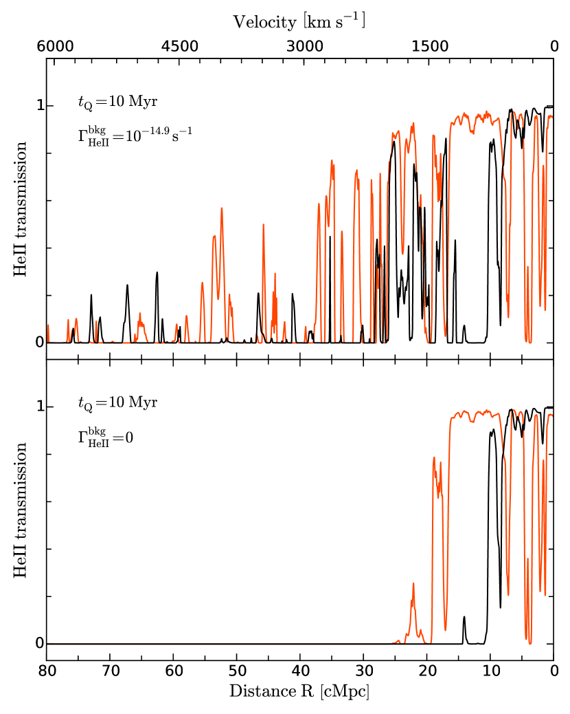
Figure 6.— He II proximity region for two different density skewers and the same model parameters (top panel: $t_{\rm Q}=10$ Myr, $\Gamma_{\rm HeII}^{\rm bkg}=10^{-14.9}{\rm s}^{-1}$, bottom panel: $t_{\rm Q}=10$ Myr, $\Gamma_{\rm HeII}^{\rm bkg}=0$). Density fluctuations alter the proximity region profile even with other parameters fixed, acting as a source of uncertainty in our analysis.

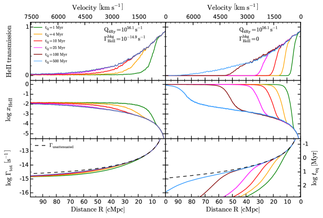
Figure 7.— Results of the radiative transfer simulations. Three panels show (from top to bottom): a) transmission profiles for different values of quasar lifetime and fixed values of $\Gamma_{\rm HeII}^{\rm bkg}=10^{-14.9}{\rm s^{-1}}$ and $Q_{\rm 4Ry}=10^{56.1}{\rm s^{-1}}$; b) evolution of the median He II fraction $x_{\rm HeII}$ for each of the models; c) total photoionization rate $\Gamma_{\rm tot}$ (dashed line corresponds to the total unattenuated photoionization rate). Left side panels show models with He II ionizing background $\Gamma_{\rm HeII}^{\rm bkg}=10^{-14.9}{\rm s}^{-1}$, while the right side panels show models with zero background, i.e., $\Gamma_{\rm HeII}^{\rm bkg}=0$. The equilibration timescale $t_{\rm eq}$ is plotted on the right $y$-axis in the bottom panel.

One approach to mitigate the impact of these density fluctuations, is to average them down by stacking different He II proximity regions, using potentially all $\sim 30$ He II Ly$\alpha$ forest sightlines observed to date (Worseck et al., 2011; Syphers et al., 2012). From the perspective of the modeling, this also helps to isolate the salient dependencies of the mean transmission profile on the model parameters. In this section, we analyze stacked He II Ly$\alpha$ profiles and study their dependence on the three parameters that govern the structure of the proximity zones: the quasar lifetime $t_{\rm Q}$, the He II ionizing background $\Gamma^{\rm bkg}_{\rm HeII}$, and the quasar photon production rate $Q_{\rm 4Ry}$.

4.1. The Dependence on Quasar Lifetime $t_{\rm Q}$

In Figure 7 we show stacks of $1000$ skewers for a sequence of proximity zone models with different quasar lifetimes in the range $t_{\rm Q}=1-500$ Myr, indicated by the colored curves, but with other parameters ($\Gamma_{\rm HeII}^{\rm bkg}$ and $Q_{\rm 4Ry}$) fixed. The panels show, from top to bottom, the stacked transmission profiles in He II Ly$\alpha$ region, the He II fraction $x_{\rm HeII}$, and the total photoionization rate $\Gamma_{\rm tot}=\Gamma_{\rm QSO}+\Gamma_{\rm HeII}^{\rm bkg}$ together with the unattenuated photoionization rate $\Gamma_{\rm unatt.}$. The panels on the left show the models with fixed values of $\Gamma_{\rm HeII}^{\rm bkg}=10^{-14.9}{\rm s^{-1}}$, whereas the right side illustrates the $\Gamma_{\rm HeII}^{\rm bkg}=0$ case. The photon production rate has been set to fiducial value $Q_{\rm 4Ry}=10^{56.1}{\rm s^{-1}}$ throughout.

Several qualitative trends are readily apparent from Figure 7. First, as was also mentioned in § 3.3, at the smallest radii $R\lesssim 5$ cMpc, there is a ‘core’ of the proximity zone, which is insensitive to the changes of the quasar lifetime such that all transmission profiles overlap. Second, it is clear that both with ($\Gamma_{\rm HeII}^{\rm bkg}=10^{-14.9}{\rm s}^{-1}$) and without ($\Gamma_{\rm HeII}^{\rm bkg}=0$) a He II ionizing background, increasing the quasar lifetime $t_{\rm Q}$ results in larger proximity zones, reflecting the longer time that the nearby IGM has been exposed to the radiation from the quasar. Third, in the presence of a He II ionizing background $\Gamma_{\rm HeII}^{\rm bkg}=10^{-14.9}{\rm s}^{-1}$, the transmission profile shape loses sensitivity to quasar lifetime for models with $t_{\rm Q}>25$ Myr, whereas for $\Gamma_{\rm HeII}^{\rm bkg}=0$ case, the proximity zone continues to grow with increasing quasar lifetime up to large values of $t_{\rm Q}=500$ Myr.

We can gain a better physical understanding of the origin of these trends from the equation that describes the time evolution of the He II fraction $x_{\rm HeII}\left(t\right)$ given by eqn. (16) and discussed in § 3.2 and § 3.3. In what follows we focus on the specific example $\Gamma_{\rm HeII}^{\rm bkg}=10^{-14.9}{\rm s}^{-1}$, but our discussion also applies to the case of zero ionizing background, provided that the equation for the time evolution is modified to account for the time-delay associated with the arrival of the ionization front (see eqn. (19) in § 3.2). At $z\sim 3$, observations of the effective optical depth strongly favor a finite background (see § 3.1) $\Gamma_{\rm HeII}^{\rm bkg}\simeq 10^{-14.9}{\rm s}^{-1}$ ($x_{\rm HeII}\simeq 10^{-2}$), although most of the previous interpretations of observed He II proximity regions have concentrated on the $\Gamma_{\rm HeII}^{\rm bkg}=0$ case (Shull et al., 2010; Syphers & Shull, 2014; Zheng et al., 2015).

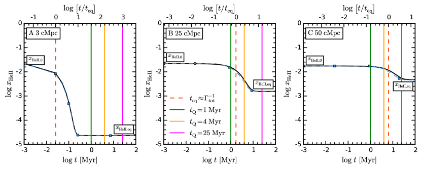
Figure 8.— Time evolution of $x_{\rm HeII}\left(t,R\right)$ at different distances from the quasar: A) $3$ cMpc, B) $25$ cMpc, and C) $50$ cMpc. Solid black and dashed blue curves show $x_{\rm HeII}\left(t,R\right)$ evolution as output from the radiative transfer algorithm and analytical approximation based on eqn. (16), respectively. Red dashed vertical lines in each panel show the equilibration time $t_{\rm eq}$ at the distance $R$; green, orange and magenta vertical lines indicate three quasar lifetimes we consider here, i.e., $t_{\rm Q}=\left[1,4,25\right]$ Myr. These calculations use our fiducial value of the He II ionizing background $\Gamma_{\rm HeII}^{\rm bkg}=10^{-14.9}{\rm s}^{-1}$, and have a photon production rate $Q_{\rm 4Ry}=10^{56.1}\,{\rm s^{-1}}$.

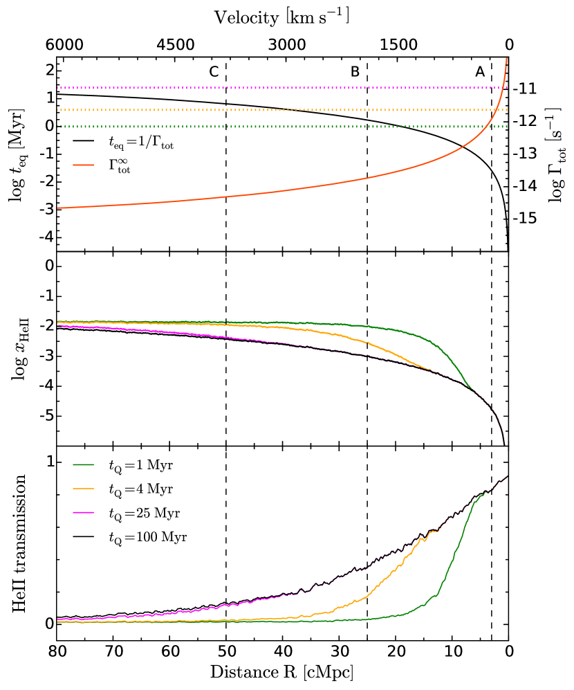
Figure 9.— Top panel: total photoionization rate $\Gamma_{\rm tot}$ as a function of distance $R$ (red) and the equilibration time $t_{\rm eq}=1/\Gamma_{\rm tot}$ (black). Dashed vertical lines correspond to the locations A,B and C in Figure 8 where we traced the time-evolution of the He II fraction. Three horizontal dotted lines in the upper panel correspond to the values of quasar lifetimes $t_{\rm Q}$ that we consider in Figure 8. Middle panel: time evolution of the He II fraction computed at $t=t_{\rm Q}=\left[1,4,25,100\right]\ {\rm Myr}$ as a function of distance $R$ from the quasar. Bottom panel: stacked transmission profiles for models with different quasar lifetimes (same as Figure 7).

The three panels in Figure 8 show the time evolution of the He II fraction at three different distances from the quasar $R=\left[3,25,50\right]$ cMpc, labeled A, B, and C, respectively. The black curves show the average $x_{\rm HeII}\left(t\right)$ computed from $100$ skewers, where the quasar was on for the entire $t_{\rm Q}=100$ Myr that is shown. The dashed blue curves show the time evolution from eqn. (16), where for the input parameters we have averaged the outputs from the radiative transfer code. Specifically, to compute the blue curves we take an average value of photoionization rate $\langle\Gamma_{\rm tot}\rangle$ which is a mean of 100 skewers and we do the same for the equilibrium $x_{\rm HeII,eq}=\langle\alpha_{\rm A}\left({\rm T}\right)n_{\rm e}\rangle/\langle\Gamma_{\rm tot}\rangle$, and initial neutral fractions $x_{\rm HeII,0}=\langle\alpha_{\rm A}\left({\rm T}\right)n_{\rm e}\rangle/\Gamma_{\rm HeII}^{\rm bkg}$ .

This procedure excellently reproduces the evolution given by the solid black curves, computed from a full time integration of the radiative transfer. Whereas we previously saw that this analytical approximation provides a good fit to the time evolution of the He II fraction of a single skewer (see Figure 4), it is somewhat surprising that it also works so well for the stacked spectra using these averaged quantities.

As Figure 8 shows the full time evolution of He II fraction over $100$ Myr, observing a quasar with a given quasar lifetime $t_{\rm Q}$ is equivalent to evaluating $x_{\rm HeII}\left(t\right)$ at the time $t=t_{\rm Q}$. The green, yellow, and magenta vertical lines indicate three possible quasar lifetimes of $t_{\rm Q}=1,\ 4,\ {\rm and}\ 25$ Myr, respectively. The spatial profile of $x_{\rm HeII}$ and Ly$\alpha$ transmission are shown in the middle and bottom panels of Figure 9 for the same three quasar lifetime models (with the same line colors as in Figure 8). The black curves in these two panels show the “equilibrium” $t=\infty$ profiles for $x_{\rm HeII}$ and the transmission, which we define to correspond to $t_{\rm Q}=100\,{\rm Myr}$, at which time $x_{\rm HeII}$ has fully equlibrated. The vertical dashed lines labeled A, B, and C in Figure 9 indicate the three distances from the quasar $R=\left[3,25,50\right]$ cMpc for which the time evolution is shown in Figure 8.

First, consider location A in the inner ‘core’ of the proximity zone at a distance of $R=3$ cMpc, at which the He II fraction and transmission profiles in Figure 9 are all identical for the quasar lifetimes we consider. The uppermost panel of Figure 9 shows the equilibration time as a function of distance from the quasar, which indicates that at $R=3\,{\rm cMpc}$ $t_{\rm eq}=0.025$ Myr. The reason why all quasar lifetimes are indistinguishable at this distance can be easily understood from the $x_{\rm HeII}\left(t\right)$ evolution in the left panel of Figure 8. Irrespective of whether the quasar has been emitting for $t_{\rm Q}=1$ Myr (green), $t_{\rm Q}=4$ Myr (yellow) or $t_{\rm Q}=16$ Myr (magenta), because at this distance the equilibration time (red vertical dashed line) $t_{\rm eq}\ll t_{\rm Q}$, the IGM has already equilibrated $x_{\rm HeII,eq}\simeq 2.5\times 10^{-5}$, and there is thus no sensitivity to quasar lifetime (see also the discussion in § 3.3 and eqn. 20).

Note however that the $t_{\rm eq}\sim R^{2}$ dependence of equilibration time shown in the top panel of Figure 9 indicates that at greater distances, the equilibration time is larger and becomes comparable to the lifetimes we consider. This manifests as significant differences in the stacked $x_{\rm HeII}$ and transmission profiles for different lifetimes in Figure 9, which can again be understood from the time evolution in Figure 8. For example, consider location B (middle panel of Figure 8) at $R=25$ cMpc, at which the equilibration time is $t_{\rm eq}=1.7$ Myr (red vertical dashed line). For the shortest quasar lifetime of $1$ Myr (green line), the IGM has not been illuminated long enough to equilibrate, i.e., $t_{\rm Q}<t_{\rm eq}$, and thus still reflects the He II fraction $x_{\rm HeII,0}$ consistent with the $\Gamma_{\rm HeII}^{\rm bkg}$ that prevailed before the quasar turned on. This $x_{\rm HeII,0}\simeq 2.2\times 10^{-2}$, much larger than the equilibrium value $x_{\rm HeII,eq}\simeq 1.5\times 10^{-3}$, explains why the corresponding transmission at location B in Figure 9 (green curve) lies far below the fully equilibrated model $t_{\rm Q}=100$ Myr (black curve). Likewise, the $t_{\rm Q}=4$ Myr model (yellow) is still in the process of equilibriating, whereas the $t_{\rm Q}=25$ Myr model (magenta) has fully equilibrated, explaining the respective values of the $x_{\rm HeII}$ and transmission for these models at location B in Figure 9.

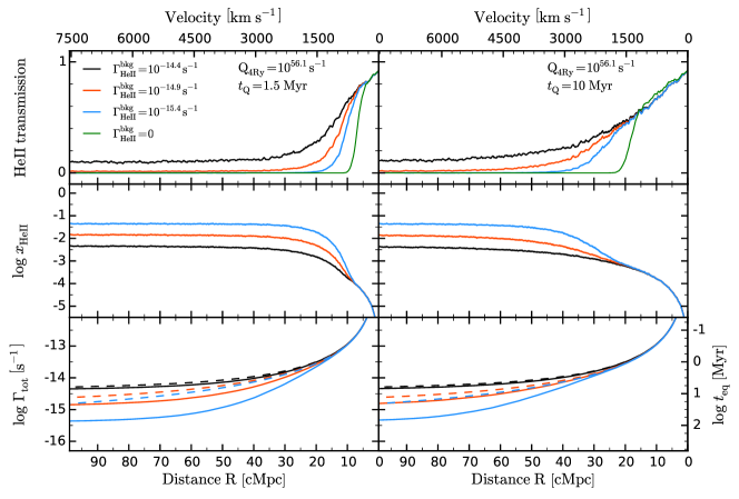
Figure 10.— Stacked proximity region trends when varying the He II ionizing background, where each curve is calculated from $1000$ skewers. Lefthand panels show three models with $\Gamma_{\rm HeII}^{\rm bkg}=\left[10^{-14.4},10^{-14.9},10^{-15.4},0\right]\ {\rm s}^{-1}$ for a quasar lifetime $t_{\rm Q}=1.5$ Myr. Righthand panels show the same models of $\Gamma_{\rm HeII}^{\rm bkg}$ but for the quasar lifetime $t_{\rm Q}=10$ Myr. All panels take a photon production rate of $Q_{\rm 4Ry}=10^{56.1}{\rm s^{-1}}$. See Figure 7 for a description of the quantities plotted on the $y$-axis.

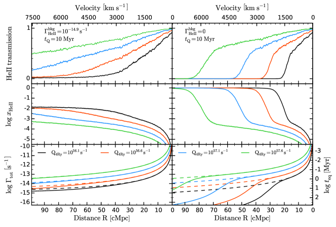
Figure 11.— Stacked proximity region trends with varying the quasar $4~{}$Ry photon production rate, ${\rm Q_{4Ry}}$, where each curve is calculated from $1000$ skewers. All curves assume a fixed quasar lifetime of $t_{\rm Q}=10$ Myr and fixed He II ionizing background $\Gamma_{\rm HeII}^{\rm bkg}$ where the lefthand panels take $\Gamma_{\rm HeII}^{\rm bkg}=10^{-14.9}{\rm s}^{-1}$ and the righthand panels take $\Gamma_{\rm HeII}^{\rm bkg}=0$ (i.e., $x_{\rm HeII}=1$). See Figure 7 for a description of the quantities plotted on the $y$-axis.

Because equilibration time increases with distance from the quasar, the stacked transmission profile becomes sensitive to larger quasar lifetimes at larger radii. This is evident from the transmission profiles in Figure 7 and Figure 9, where models with progressively larger lifetimes peel off from the equilibrium model ($t_{\rm Q}=100$ Myr) at progressively larger radii. However, eventually far from the quasar, this sensitivity saturates, as $t_{\rm eq}$ approaches its asymptotic value $t_{\rm eq}\sim 1/\Gamma_{\rm HeII}^{\rm bkg}$ (see upper panel of Figure 9), which for our fiducial $\Gamma_{\rm HeII}^{\rm bkg}=10^{-14.9}{\rm s}^{-1}$ corresponds to $t_{\rm eq}=25$ Myr. This saturation effect is illustrated by the time evolution at location C, $R=50$ cMpc from the quasar, in the right panel of Figure 8. If the quasar has been illuminating the IGM for $t_{\rm Q}=25$ Myr (magenta curve), the He II fraction has nearly reached equilibrium $x_{\rm HeII,eq}$, and thus at location C Figure 9 exhibits only a small but still noticeable difference between the $x_{\rm HeII}$ at $t_{\rm Q}=25$ Myr and the equilibrium model (black curve), and consequently the transmission profiles (lower panel) hardly differ at all. It would clearly be extremely challenging to distinguish between different models with $t_{\rm Q}>25$ Myr. Finally, at the largest radii $R>R_{\rm bkg}=70$ cMpc, where $R_{\rm bkg}$ is defined to be the location where $\Gamma_{\rm HeII}^{\rm bkg}=\Gamma_{\rm QSO}$, the quasar no longer dominates over the background, and all the transmission profiles converge to the mean transmission set by the He II background. Finally, we again note that if $\Gamma_{\rm HeII}^{\rm bkg}=0$, there is no such asymptote in the equilibration time, and the transmission profile continues to be sensitive to values of quasar lifetime as large as $t_{\rm Q}=500$ Myr as shown in Figure 7. However, in practice for very long quasar lifetimes and therefore very large proximity zones, one might eventually encounter locations in the universe where the background is no longer zero.

4.2. The Dependence on the He II background $\Gamma_{\rm HeII}^{\rm bkg}$

In Figure 10 we illustrate the impact of varying the He II ionizing background $\Gamma_{\rm HeII}^{\rm bkg}$ on the stacked transmission profile, with $t_{\rm Q}$ and $Q_{\rm 4Ry}$ held fixed. The left panels show a quasar lifetime of $t_{\rm Q}=1.5$ Myr, whereas the right show $t_{\rm Q}=10$ Myr. Four different values for $\Gamma_{\rm HeII}^{\rm bkg}$ are plotted, including the $\Gamma_{\rm HeII}^{\rm bkg}=0$ case.

From Figure 10, we see that in the inner core $R<5\,{\rm cMpc}$ of the proximity zone, the transmission profile is independent of $\Gamma_{\rm HeII}^{\rm bkg}$, analogous to the behavior in Figure 7, where we saw that the core is also independent of $t_{\rm Q}$. As discussed in § 3.3 (see also the previous section), this insensitivity to $\Gamma_{\rm HeII}^{\rm bkg}$ and $t_{\rm Q}$ can be understood from eqn. (20) governing the time evolution of $x_{\rm HeII}$. For $t_{\rm eq}\ll t_{\rm Q}$, the IGM has already equilibrated and $x_{\rm HeII}(t_{\rm Q})\approx x_{\rm HeII,eq}$. At small distances $R\ll R_{\rm bkg}$ the quasar dominates over the background $\Gamma_{\rm QSO}\gg\Gamma_{\rm HeII}^{\rm bkg}$ and attenuation is negligible, hence the equilibrium He II fraction $x_{\rm HeII,eq}\propto\Gamma_{\rm QSO}^{-1}$ is determined by the quasar photon production rate alone, and is independent of the background and quasar lifetime.

In the previous section we argued that the equilibration time picture explains why the transmission profiles for progressively larger lifetimes peel off from the equilibrium model ($t_{\rm Q}=100$ Myr) at progressively larger radii (see Figure 7). The curves in Figure 10 illustrate that varying the ionizing background has a different effect, namely to change the slope of the transmission profile about this peel off point, as well as to determine the transmission level far from quasar. The different response of the transmission profile to these two parameters, $t_{\rm Q}$ and $\Gamma_{\rm HeII}^{\rm bkg}$, results from the functional form of eqn. (20). The stronger peel off behavior with $t_{\rm Q}$ is due to the exponential dependence on the quasar lifetime $t_{\rm Q}$ in eqn. (20), whereas the milder variation of the slope with $\Gamma_{\rm HeII}^{\rm bkg}$ arises because of the inverse proportionality of $x_{\rm HeII,eq}$ on $\Gamma_{\rm HeII}^{\rm bkg}$. Furthermore, at large distances from the quasar where $\Gamma_{\rm tot}\simeq\Gamma_{\rm HeII}^{\rm bkg}$, $x_{\rm HeII,eq}$ approaches $x_{\rm HeII,0}\propto 1/\Gamma_{\rm HeII}^{\rm bkg}$ and the background sets the absorption level as expected. As we also noted in § 3.3, the different dependence of the transmission profile on $t_{\rm Q}$ and $\Gamma_{\rm HeII}^{\rm bkg}$ suggests that the degeneracy between these parameters could be broken by the shape of the transmission profile, which we discuss further in § 5.2.

4.3. The Dependence on the Photon Production Rate $Q_{\rm 4Ry}$

Figure 11 shows the effect of the photon production rate on the structure of the proximity zone. The quasar lifetime has been set to the value $t_{\rm Q}=10$ Myr, and the background is $\Gamma_{\rm HeII}^{\rm bkg}=10^{-14.9}{\rm s}^{-1}$ on the left and $\Gamma_{\rm HeII}^{\rm bkg}=0$ on the right. One can see that the impact of the photon production rate $Q_{\rm 4Ry}$ on the resulting transmission profile is twofold. First, as expected, more luminous quasars produce larger proximity zones, i.e., increasing the photon production rate by $0.5$ dex expands the characteristic size of the proximity zone by a factor of $\sim 2$. Second, besides increasing the overall size, the slope of the stacked transmission profile becomes shallower when $Q_{\rm 4Ry}$ is increased.

The increase in proximity zone size with $Q_{\rm 4Ry}$ can be easily understood in the equilibration time picture. From eqn. (22), we see that the equilibration distance $R_{\rm eq}$, which sets the location where the transmission profile becomes sensitive to $t_{\rm Q}$ and approaches the mean transmission level of the IGM (see Figure 7), scales as $R_{\rm eq}\propto Q_{\rm 4Ry}^{1/2}$. Hence an increase (decrease) in photon production rate $Q_{\rm 4Ry}$ results in a larger (smaller) characteristic size of the proximity zone.

To understand the change in transmission profile slope with $Q_{\rm 4Ry}$, consider that in the core of the proximity zone where $t_{\rm eq}\ll t_{\rm Q}$, the He II fraction has equilibrated and is given by $x_{\rm HeII}\left(t\right)=x_{\rm HeII,eq}$, where $x_{\rm HeII,eq}\propto Q_{\rm 4Ry}^{-1}$. As the transmitted flux is just the exponential of a constant times $x_{\rm HeII,eq}$, an increase (decrease) in $Q_{\rm 4Ry}$ makes this exponent smaller (larger) and thus the slope of the transmission profile becomes shallower (steeper).

4.4. The Dependence on the spectral slope $\alpha$

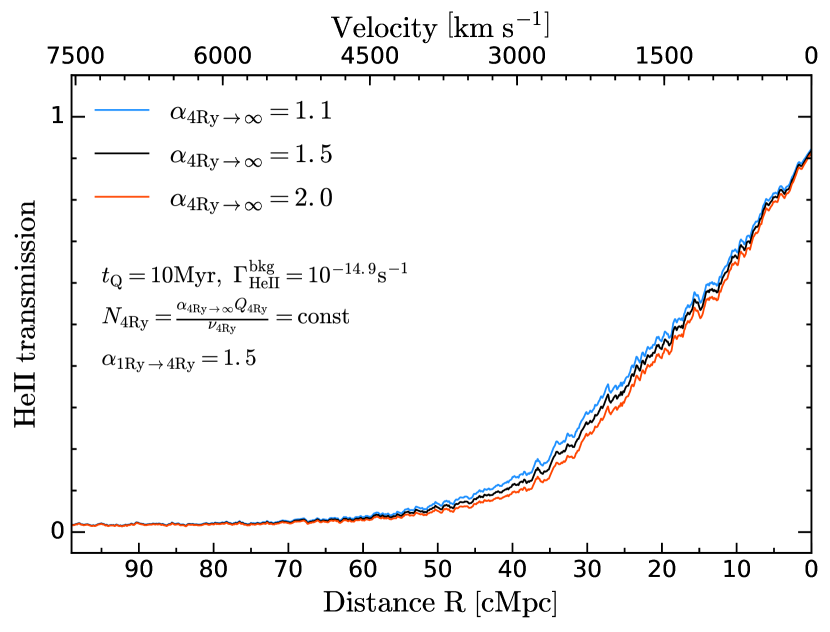
Figure 12.— Stacked proximity region trends with varying the slope of quasar SED above $4$ Ry, $\alpha_{\rm 4Ry\rightarrow\infty}$, where each curve is calculated from $1000$ skewers. All curves assume a fixed quasar lifetime of $t_{\rm Q}=10$ Myr and fixed He II ionizing background $\Gamma_{\rm HeII}^{\rm bkg}=10^{-14.9}{\rm s}^{-1}$.

As we illustrated in § 2.2, the total quasar photon production rate $Q_{\rm 4Ry}$ at frequencies above the He II ionization threshold depends on the assumed slope of the quasar SED $\alpha$ blueward of $4$ Ry. Throughout the paper we have assumed that $\alpha=1.5$ is constant at all frequencies blueward of $1$ Ry and simply varied the value of $Q_{\rm 4Ry}$ to illustrate its effect on the stacked transmission profiles (see § 4.3). However, the spectral slope regulates the number of hard photons with long mean free path which can affect the transmission profiles at large distances from the quasar. Therefore, it is not obvious whether $Q_{\rm 4Ry}$ and $\alpha$ impact the structure of the proximity zone in the same way.

We thus run a set of radiative transfer simulations to further explore this question. In order to disentangle the effects of $Q_{\rm 4Ry}$ and $\alpha$ on the transmission profiles we chose to fix the quasar specific luminosity $N_{\rm 4Ry}$ at $4$ Ry (see eqn. 1), which can be deduced from the observable quasar specific luminosity at the H I ionization threshold of $1$ Ry by scaling it down to He II ionization threshold with constant spectral slope $\alpha_{\rm 1Ry\rightarrow 4Ry}=1.5$. We then freely vary the spectral slop $\alpha_{\rm 4Ry\rightarrow\infty}$ within the range $\alpha_{\rm 4Ry\rightarrow\infty}=1.1-2.0$. Although, the actual slope of quasar SED at $\lambda\leq 912{\rm\AA}$ is not currently well known, the chosen range of $\alpha_{\rm 4Ry\rightarrow\infty}$ values is motivated by the constraints on the power-law index from Lusso et al. (2015), who found $\alpha_{\nu}=1.70\pm 0.61$ at $\lambda\leq 912{\rm\AA}$.

Figure 12 illustrates the effect of the spectral slope on the structure of the proximity zone. The quasar lifetime and He II background are fixed at $t_{\rm Q}=10$ Myr and $\Gamma_{\rm HeII}^{\rm bkg}=10^{-14.9}{\rm s^{-1}}$, respectively. Three curves show stacked transmission profiles for our fiducial value $\alpha_{\rm 4Ry\rightarrow\infty}=1.5$ (black), harder slope $\alpha_{\rm 4Ry\rightarrow\infty}=1.1$ (blue), and softer slope $\alpha_{\rm 4Ry\rightarrow\infty}=2.0$ (red). It is apparent from Figure 12 that the effect of the spectral slope on the structure of the proximity zone is negligible in comparison to the effect of the overall photon production rate $Q_{\rm 4Ry}$ (see Figure 11).

Consider that when specific luminosity $N_{\rm 4Ry}$ is fixed at $4{\rm Ry}$, the quasar photon production rate $Q_{\rm 4Ry}$ scales with $\alpha_{\rm 4Ry\rightarrow\infty}$ as $Q_{\rm 4Ry}\propto\alpha_{\rm 4Ry\rightarrow\infty}^{-1}$ (see eqn. 1). Thus, varying the value of $\alpha_{\rm 4Ry\rightarrow\infty}$, results in $25-45\%$ changes in the photon production rate $Q_{\rm 4Ry}$ (which is the ratio of assumed spectral slopes $\alpha_{\rm 4Ry\rightarrow\infty}$ in different models). Thus, one would expect a significant difference in the resulting transmission according to Figure 11. However, the more important quantity here is the cross-section weighted quasar He II photoionization rate $\Gamma_{\rm QSO}$ given by eqn. (3), which regulates the time-evolution of the He II fraction (and, consequently, the transmission profile). Since the ionization cross-section scales as $\sigma_{\nu}\propto\left(\nu/\nu_{\rm th}\right)^{-3}$, the resulting dependence of the He II photoionization rate in the unattenuated limit on the spectral slope is $\Gamma_{\rm QSO}\propto\left(\alpha_{\rm 4Ry\rightarrow\infty}+3\right)^{-1}$. Hence, the difference between the photoionization rates of the fiducial model $\alpha_{\rm 4Ry\rightarrow\infty}=1.5$ and the two models in Figure 12 with $\alpha_{\rm 4Ry\rightarrow\infty}=1.1$ and $\alpha_{\rm 4Ry\rightarrow\infty}=2.0$ is only $\Delta\Gamma\approx 10\%$. Therefore, there is no significant effect in the resulting transmission in He II proximity zone even for relatively large variations in the assumed spectral slope of quasar SED blueward of $4$ Ry.

5. Discussion

In the previous section we assumed only single values of quasar lifetime and He II background when exploring their impact on the stacked transmission profiles. However, this approach is probably too simplistic because in reality these parameters are expected to vary. The He II background will fluctuate from one line-of-sight to another due to the density fluctuations. Analogously, quasars will also have a distribution of the lifetimes. Moreover, the complete reionization of intergalactic helium is a temporally extended process. Thus, the conditions in the IGM will evolve and might affect the sensitivity of our models to the quasar and IGM parameters. Therefore, in this section we want to: $\left(1\right)$ check if the results we obtained in previous sections still hold if we consider more realistic models with a distribution of quasar lifetimes and He II ionizing backgrounds as one expects to encounter in the universe, and $\left(2\right)$ check if our results are valid at higher redshifts where the He II ionizing background cannot be determined from effective optical depth measurements.

In what follows we consider two diagnostic methods. First, we use the same stacked transmission profiles that we discussed in previous sections. Second, we study the distribution of the He II proximity zone sizes, the statistics that has been previously used in the literature to characterize high-redshift H I and He II proximity zones.

5.1. The Effect of the Distribution of Quasar Lifetimes and He II Backgrounds on the stacked Transmission Profiles

In what follows we study the impact of the distribution of quasar lifetimes and He II backgrounds on the shape of the stacked transmission profiles in He II Ly$\alpha$ regions at $z=3.1$ using the same stacking technique described in § 4.

First, we consider the distribution of quasar lifetimes only, while keeping He II background and quasar photon production rate fixed to our fiducial values $\Gamma_{\rm HeII}^{\rm bkg}=10^{-14.9}{\rm s^{-1}}$ and $Q_{\rm 4Ry}=10^{56.1}{\rm s^{-1}}$, respectively. The upper panel of Figure 13 shows the comparison between the stacked transmission profiles of our fiducial model with single quasar lifetime $t_{\rm Q}=10$ Myr and three models with different distributions of $t_{\rm Q}$. We model the distribution of quasar lifetimes as a uniform sampling from $5$ discrete $t_{\rm Q}$ values centered on ${\rm log}\ (t_{\rm Q}/{\rm Myr})=1.00$ spanning a total range of $0\leq{\rm log}\ (t_{\rm Q}/{\rm Myr})\leq 2$, but with different widths $\Delta{\rm log}\ (t_{\rm Q}/{\rm Myr})=\left[0.5,1.0,2.0\right]$. This is done by constructing stacks of $1000$ skewers, where each skewer is randomly chosen from one of the single lifetime models over the range specified by the width. The blue curve in the upper panel of Figure 13 represents the stack of skewers taken from models with ${\rm log}\ \left(t_{\rm Q}/{\rm Myr}\right)=\left[0.75,0.875,1.00,1.125,1.25\right]$, red is a stack of skewers with ${\rm log}\ \left(t_{\rm Q}/{\rm Myr}\right)=\left[0.50,0.75,1.00,1.25,1.50\right]$ and green is ${\rm log}\ \left(t_{\rm Q}/{\rm Myr}\right)=\left[0.00,0.50,1.00,1.50,2.00\right]$. The numbers in square brackets represent the values of $t_{\rm Q}$ or $\Gamma_{\rm HeII}^{\rm bkg}$ (see below) used in the models that contributed to the stacks of the distribution models.

The upper panel of Figure 13 clearly shows that in comparison to the single lifetime model, there appears to be a reduction in the transmission in the range $R\simeq 10-40$ cMpc in the stacked spectra of models with the distribution of quasar lifetimes. This is due to the skewers with lower values of $t_{\rm Q}$. In these models the IGM did not have enough time to respond to the changes in the radiation field caused by the quasar and still reflects a higher He II fraction set by the He II ionizing background, resulting in decreased transmission. Furthermore, the transmission becomes more depressed as the width of the quasar lifetime distribution increases, indicating that stacked transmission profiles are also sensitive to the width of the quasar lifetime distribution.

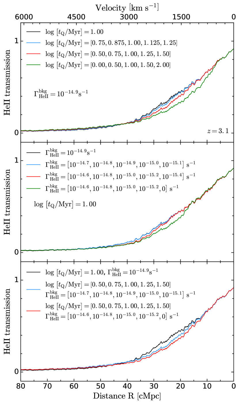
Figure 13.— Top panel: effect of the quasar lifetime distribution on the stacked transmission profile. The He II background is fixed for all models to $\Gamma_{\rm HeII}^{\rm bkg}=10^{-14.9}{\rm s^{-1}}$. Each of the curves represents a stack of $1000$ skewers. The black curve shows the stacked profile of the model with single value of quasar lifetime $t_{\rm Q}=10$ Myr, while other curves correspond to the stacked profiles of the models that take distribution of $t_{\rm Q}$ with different widths: ${\rm log}\ (t_{\rm Q}/{\rm Myr})=\left[0.75,0.875,1.00,1.125,1.25\right]$ (blue), ${\rm log}\ (t_{\rm Q}/{\rm Myr})=\left[0.50,0.75,1.00,1.25,1.50\right]$ (red), ${\rm log}\ (t_{\rm Q}/{\rm Myr})=\left[0.00,0.50,1.00,1.50,2.00\right]$ (green). Middle panel: The same, but for distribution of He II backgrounds. Quasar lifetime is fixed to ${\rm log}\ (t_{\rm Q}/{\rm Myr})=1.00$. The black curve has a fiducial value of $\Gamma_{\rm HeII}^{\rm bkg}=10^{-14.9}{\rm s^{-1}}$, and other curves take the distribution of backgrounds, i.e., $\Gamma_{\rm HeII}^{\rm bkg}=\left[10^{-14.7},10^{-14.8},10^{-14.9},10^{-15.0},10^{-15.1}\right]{\rm s^{-1}}$ (blue), $\Gamma_{\rm HeII}^{\rm bkg}=\left[10^{-14.6},10^{-14.8},10^{-15.0},10^{-15.2},10^{-15.4}\right]{\rm s^{-1}}$ (red), and $\Gamma_{\rm HeII}^{\rm bkg}=\left[10^{-14.6},10^{-14.8},10^{-15.0},10^{-15.2},0\right]{\rm s^{-1}}$ (green). Bottom panel: The combined effect of the distributions of quasar lifetimes and He II backgrounds.

Similarly, we now investigate how the distribution of He II backgrounds affects the stacked transmission profiles. As we discussed in § 3.1, our fiducial value of He II background $\Gamma_{\rm HeII}^{\rm bkg}=10^{-14.9}{\rm s^{-1}}$ is derived from measurements of the He II effective optical depth $\tau_{\rm eff}$ which give $\tau_{\rm eff}\simeq 4.5$ at $z=3.1$ (see Figure 3). Therefore, the distribution of He II ionizing backgrounds should also correspond to the same observed mean effective optical depth of $\tau_{\rm eff}\simeq 4.5$. Analogously to § 3.1, we run our radiative transfer calculation with the quasar turned off for $100$ skewers chosen from several models with different values of the He II background. We focus on two uniform distributions for $\Gamma_{\rm HeII}^{\rm bkg}$ which yield the same effective optical depth $\tau_{\rm eff}\simeq 4.5$: $\Gamma_{\rm HeII}^{\rm bkg}=\left[10^{-14.7},10^{-14.8},10^{-14.9},10^{-15.0},10^{-15.1}\right]{\rm s^{-1}}$ and $\Gamma_{\rm HeII}^{\rm bkg}=\left[10^{-14.6},10^{-14.8},10^{-15.0},10^{-15.2},10^{-15.4}\right]{\rm s^{-1}}$. We then run our $1$D radiative transfer algorithm with the quasar on for $t_{\rm Q}=10$ Myr and calculate $10$ different models with the above mentioned values of He II background. Similar to the distribution of quasar lifetimes, we calculate two stacked transmission profiles using $1000$ skewers randomly chosen from these models.

The results of this exercise are shown in the middle panel of Figure 13, where the black curve corresponds to the model with a single value of He II background fixed at our fiducial value of $\Gamma_{\rm HeII}^{\rm bkg}=10^{-14.9}{\rm s^{-1}}$, the blue curve shows the model with a background distribution that spans a range of $0.4$ dex $\Gamma_{\rm HeII}^{\rm bkg}=\left[10^{-14.7}-10^{-15.1}\right]{\rm s^{-1}}$, and the red curve is for the model spanning $0.8$ dex $\Gamma_{\rm HeII}^{\rm bkg}=\left[10^{-14.6}-10^{-15.4}\right]{\rm s^{-1}}$. We also include a model in which $20\%$ of the IGM at $z\simeq 3$ is still represented by the regions with $x_{\rm HeII}=1$, or, equivalently, $\Gamma_{\rm HeII}^{\rm bkg}=0$, which is shown in the middle panel of Figure 13 by the green curve. It is apparent that for the distributions we consider here, varying the He II background such that the mean effective optical depth is fixed, has only a small effect on the resulting transmission profile. However, if measurements of the He II effective optical depth cannot rule out the existence of the regions of IGM with high fractions of singly ionized helium, including them into the distribution of backgrounds can produce a stronger effect on the stacked transmission profile. Nevertheless, comparing to the upper panel of Figure 13 we can conclude that the distribution of quasar lifetimes has a dominant effect on the stacked transmission profile and future attempts to model stacked proximity zone should take this into account. This is illustrated in the bottom panel of Figure 13 where we combine these effects and model both the distributions of quasar lifetimes $t_{\rm Q}$ and He II backgrounds $\Gamma_{\rm HeII}^{\rm bkg}$ simultaneously, by combining skewers drawn from different models in both parameters. Note, that even in the model where $20\%$ of IGM has $\Gamma_{\rm HeII}^{\rm bkg}=0$ ($x_{\rm HeII}=1$), when convolved with a broad distribution of quasar lifetimes, the impact of these regions with $x_{\rm HeII}=1$ is not very significant.

In § 4 we showed that variations in the quasar lifetime and He II background impact stacked transmission profiles in distinct ways. Our analysis here shows that the width of the distribution of quasar lifetimes, can significantly change the shape of the stacked transmission profile, and should be included in any attempt to model real observations. Nevertheless, we argue that that at $z\simeq 3.1$ one should be able to put interesting constraints on the quasar lifetime given that the average He II background can be determined from the level of transmission in the IGM as quantified by effective optical depth measurements (see Figure 3 in § 3.1), and due to the fact that the stacked transmission profile is relatively insensitive to fluctuations in the He II background.

5.2. Sensitivity to the Quasar Lifetime and He II Background at Higher Redshifts

Recall Figure 3, where the blue curve shows the evolution of the mean He II effective optical depth $\tau_{\rm eff}$ and the mean He II fraction at $z=3.9$ in our simulations. At this higher redshift, the $\tau_{\rm GP}\propto(1+z)^{3/2}$ dependence of the optical depth, implies that even backgrounds which correspond to a IGM with on average relatively low He II fraction of only $\simeq 0.03-0.04$, correspond to very large effective optical depth is $\tau_{\rm eff}\simeq 8-9$. Thus, unlike the situation at $z\simeq 3$, it would be extremely challenging to measure an optical depth that high with HST/COS, making it virtually impossible to measure the He II background and thus distinguish between IGM with low He II fraction ($x_{\rm HeII}<0.05$) and the high He II fraction ($x_{\rm HeII}=1$) at $z\simeq 4$. It is, therefore, interesting to explore whether the shape of the transmission profile of He II proximity zones can be used to independently probe both the quasar lifetime and the He II background at $z\sim 4$, where the background cannot be independently constrained.

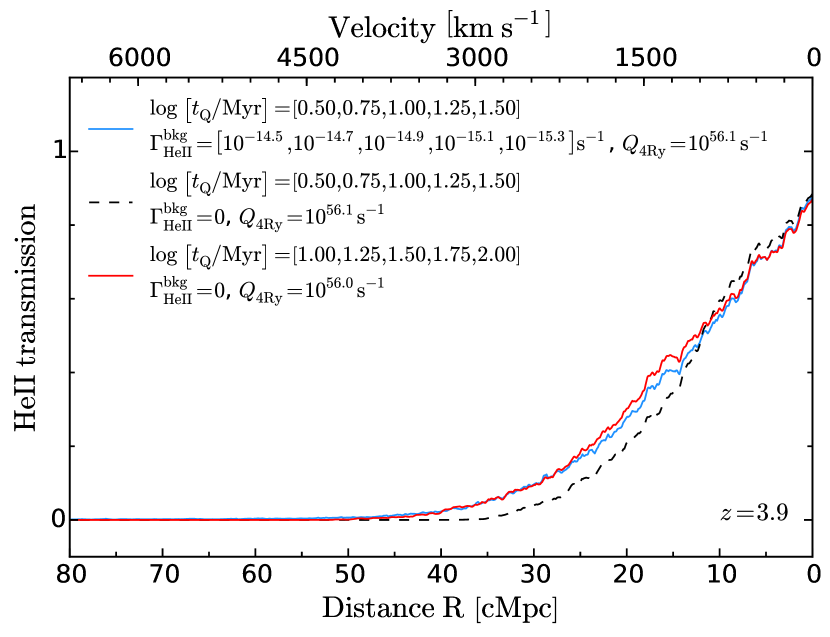
Figure 14.— Comparison between the stacked finite He II background model with $\Gamma_{\rm HeII}^{\rm bkg}=\left[10^{-14.5},10^{-14.7},10^{-14.9},10^{-15.1},10^{-15.3}\right]\ {\rm s^{-1}}$, ${\rm log}\ (t_{\rm Q}/{\rm Myr})=\left[0.50,0.75,1.00,1.25,1.50\right]$ (solid blue curve) and zero He II background models ($x_{\rm HeII}=1$ initially) with the same quasar lifetime distribution (dashed black curve). Both models have a fiducial value of photon production rate $Q_{\rm 4Ry}=10^{56.1}{\rm s^{-1}}$. The solid red curve shows the model with ${\rm log}\ (t_{\rm Q}/{\rm Myr})=\left[1.00,1.25,1.50,1.75,2.00\right]$ and reduced photon production rate $Q_{\rm 4Ry}=10^{56.0}{\rm s^{-1}}$. All calculations are performed at quasar redshift $z=3.9$.

We begin by applying our method to skewers drawn from the same hydrodynamical simulation at redshift $z=3.9$. Following our approach in the previous subsection, we choose a finite background model with uniform distribution $\Gamma_{\rm HeII}^{\rm bkg}=\left[10^{-14.5},10^{-14.7},10^{-14.9},10^{-15.1},10^{-15.3}\right]{\rm s^{-1}}$. For the distribution of lifetimes we adopt ${\rm log}\ (t_{\rm Q}/{\rm Myr})=\left[0.50,0.75,1.00,1.25,1.50\right]$, and fix the photon production rate to $Q_{\rm 4Ry}=10^{56.1}{\rm s^{-1}}$. The resulting stacked transmission profile is shown by the blue curve in Figure 14. Despite the finite background and relatively small average He II fraction $\langle x_{\rm HeII}\rangle\simeq 0.05$, far from the quasar $R>50$ cMpc, the average transmission is very nearly zero reflecting the large effective optical depth $\tau_{\rm eff}\simeq 8-9$ for this model. The dashed black curve in Figure 14 shows the stacked transmission profile for a model with the same distribution of quasar lifetimes, but with $\Gamma_{\rm HeII}^{\rm bkg}=0$ and hence an IGM with $\langle x_{\rm HeII}\rangle=1.0$, and $Q_{\rm 4Ry}$ fixed to the same value. In the absence of the He II background, one sees that the proximity zone is smaller, and the transmission approaches zero at smaller distance from the quasar than for the finite background model. This significant difference in the transmission profile naively suggests that proximity zones can be used to determine the value of the background.

However, clearly one way of compensating for this difference between the transmission profiles is to consider: $1$) a distribution with longer quasar lifetimes and, $2$) a change in the quasar photon production rate $Q_{\rm 4Ry}$, for the zero background model. Both of these parameter variations change the size of the proximity zone, which could make the two models look more similar. In principle the photon production rate $Q_{\rm 4Ry}$ should be determined by our knowledge of the quasar magnitudes, however in practice the average quasar SED is not well constrained at energies above $4$ Ry, giving rise to at least $\sim 50\%$ relative uncertainty in $Q_{\rm 4Ry}$ (see e.g. Lusso et al., 2015). To illustrate these parameter degeneracies, we increase the values of $t_{\rm Q}$ in our distribution for the zero background model by $0.50$ dex to ${\rm log}\ (t_{\rm Q}/{\rm Myr})=\left[1.00,1.25,1.50,1.75,2.00\right]$, and simultaneously slightly reduce the value of the photon production rate by $0.1$ dex to $Q_{\rm 4Ry}=10^{56.0}{\rm s^{-1}}$. The result of this exercise is shown by the solid red curve in Figure 14, which shows that the the transmission profiles for a highly doubly ionized helium ($\langle x_{\rm HeII}\rangle=0.05$) and a completely singly ionized helium ($\langle x_{\rm HeII}\rangle=1.0$) are essentially indistinguishable.

In conclusion we see, that at $z\sim 4$ the limited sensitivity of HST/COS combined with the steep rise of effective optical depth with redshift (see Figure 3), implies that one will likely only be able to place lower limits on the the average effective optical depth $\tau_{\rm eff}$, and hence upper limits on the value of the He II background. The two very different models that we considered for the He II background in Figure 14 are expected to be consistent with such limits. Without an independent measurement on the He II background, and given our poor knowledge of the SEDs of quasars above 4 Ryd, the similarity of the models in Figure 14 (blue and red curves) illustrate that it will be extremely challenging to break the degeneracies between quasar lifetime, ionizing background, and photon production rate, given existing data or even data that might be collected in the future with HST/COS. Thus, in contrast with $z\sim 3$, where an independent determination of the the He II background from effective optical depth measurements allows one to infer the quasar lifetime from proximity zones, the proximity zones of $z\sim 4$ quasars alone cannot independently constrain the quasar lifetime and ionization state of the IGM. Nevertheless, a degenerate combination of these parameters would still be extremely informative, and could be combined with other measurements to yield tighter constraints.

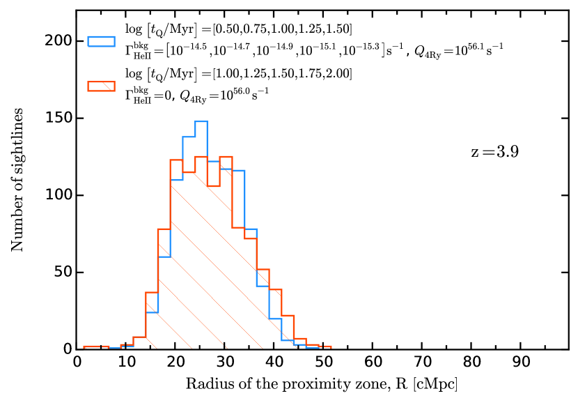
Figure 15.— Distribution of the He II proximity zone sizes measured from radiative transfer calculations on $1000$ skewers. The models are the same as in Figure 14. The size of the proximity zone is defined as the location where the smoothed spectra crosses the threshold $F=0.1$ (see text for details). The overlap of the histograms makes it impossible to precisely distinguish one model from another.

5.3. Distribution of the Proximity Zone Sizes

Previous studies of H I proximity zones at $z\simeq 6$ have concentrated on the location of the ‘edge’ of the ionized regions in order to infer the unknown parameters governing proximity zones. In this section we adopt a similar technique to investigate if it is a better diagnostic tool than stacking, considered in the previous section, for constraining the properties of the IGM and quasars at $z=3.9$.

We follow previous conventions (Fan et al., 2006) and define the size of the He II proximity zone to be the location where the appropriately smoothed transmission profile crosses the threshold value $F=0.1$ for the first time. For the choice of smoothing we follow conventions that have been adopted in the study of H I proximity zones at $z\sim 6$ (Fan et al., 2006; Carilli et al., 2010; Bolton & Haehnelt, 2007a; Lidz et al., 2007). Specifically, following the work of Fan et al. (2006), these studies smooth the spectra by a Gaussian filter with ${\rm FWHM=20\AA}$ in the observed frame, which corresponds to a velocity interval $\Delta v\sim 700\ {\rm km\ s^{-1}}$ or proper distance $R_{\rm prop}\simeq 0.97$ Mpc. We adopt the same value of the smoothing scale in proper units $R_{\rm prop}^{z=3.9}=0.97$ Mpc, which corresponds to a comoving scale of $R_{\rm com}=4.75$ cMpc at $z=3.9$, or a velocity interval $\Delta v\sim 410\,{\rm km\,s^{-1}}$. This is approximately twice the FWHM of HST/COS (for G140L grating).

Figure 15 shows the distribution of the proximity zone sizes determined in this way measured from a set of $1000$ skewers for the two models shown in Figure 14 whose stacked spectra were degenerate. Given the large degree of overlap between the histograms for these two models, and the relatively small number $\simeq 8$ of $z\gtrsim 3.5$ quasars with HST/COS spectra it is clear that it will be extremely challenging to measure the value of quasar lifetime or He II background using this definition of the proximity zone size. In § 4 we discussed how density fluctuations also introduce scatter in the distribution of the proximity zone sizes and thus complicate our ability to infer parameters (see Figure 6). We conclude that this statistical approach of measuring the sizes of He II proximity zones does not result in higher sensitivity to the properties of quasars or the IGM parameters at high redshift $z\sim 4$.

6. Mock Observations

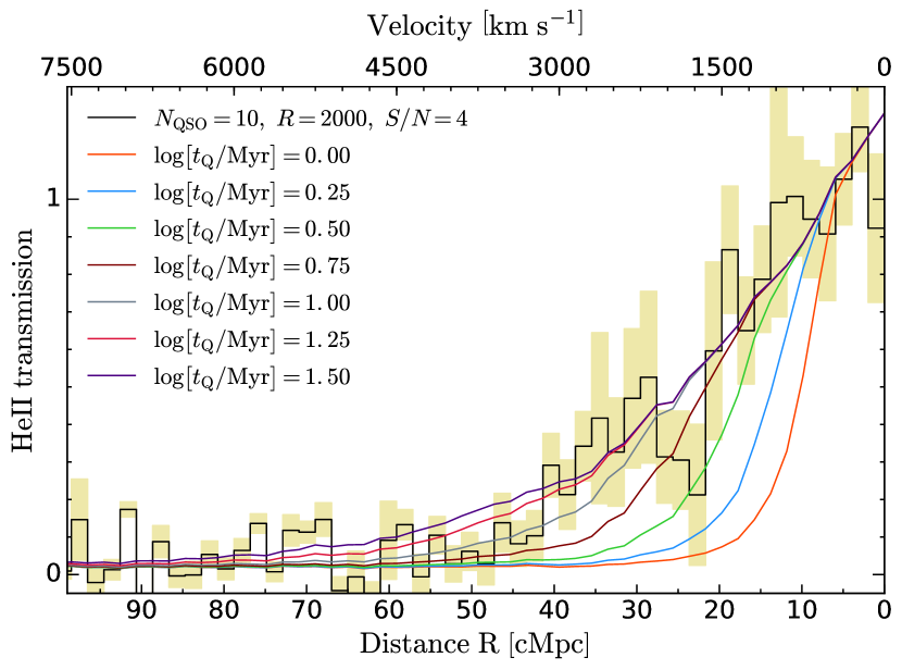
Figure 16.— Comparison of the mock observed He II proximity zones to the results of radiative transfer simulations. The histogram shows the stack of $10$ simulated skewers from our fiducial model with $t_{\rm Q}=10$ Myr, $\Gamma_{\rm HeII}^{\rm bkg}=10^{-14.9}{\rm s^{-1}}$ and $Q_{\rm 4Ry}=10^{56.1}{\rm s^{-1}}$. The resolution of each skewer has been reduced to $R=2000$ to match low-resolution HST/COS data, the noise has been added with resulting $S/N=4$. The yellow shaded area shows 1-$\sigma$ errorbars calculated via bootstrapping. Models with different values of quasar lifetime $t_{\rm Q}$ consist of $1000$ skewers also reduced to the same resolution.

In order to get a feeling for the the constraints on quasar lifetime $t_{\rm Q}$ that can be obtained with existing samples of He II proximity zone spectra (Worseck et al., 2011, 2014; Syphers et al., 2012) we perform a simple comparison of our model stacked transmission profiles to a mock observational dataset. Specifically, we randomly select $10$ skewers from our fiducial model with $t_{\rm Q}=10$ Myr and mock up the properties of real HST/COS data by convolving these spectra with a Gaussian line-spread function matched to HST/COS moderate resolution spectra $R=\lambda/\Delta\lambda=2000$ or FWHM=$150~{}{\rm km~{}s^{-1}}$ (comparable to the G140L grating). We also add Gaussian distributed noise to each spectrum assuming a constant signal-to-noise ratio $S/N=4$. The black histogram in Figure 16 shows the resulting stacked transmission profile in the He II proximity zone region. We also calculate 1-$\sigma$ errorbars for this mock dataset using the bootstrap technique, which is illustrated by the yellow shaded area. We then compare the stack with several simulated models with different values of $t_{\rm Q}$ ($1000$ skewers per model with the same resolution of $R=2000$). It is apparent from the example shown in Figure 16 that we should be able to measure the quasar lifetime within a factor of $\sim 2-3$ uncertainty.

We plan to use the method described in this paper for the follow-up analysis of real observational data. However, there is a range of uncertainties that can complicate the estimation of average quasar lifetime from the stacked transmission profiles. First, in order to stack quasar spectra one needs to take care of the flux normalization, which depends on the fitted quasar continuum. Statistical errors on the power-law fit to the quasar continuum in the He II Ly$\alpha$ forest are typically few per cent for the low $S/N$ spectra (Worseck et al., 2011, 2014). However, given the large variance indicated by the yellow shaded region in Figure 16, continuum errors will not significantly impact our results since flucutations in the IGM dominate the scatter. Similarly, the spectral resolution does not affect our constraints on quasar lifetime because we choose to stack individual spectra. Thus, we are more interested in the information contained in the shape and the slope of the stacked transmission profile, but not the individual absorption lines in the He II Ly$\alpha$ forest. In addition, large errors in the quasar systemic redshift that result from using rest-frame UV emission lines (typical uncertainties are $500-1000\ {\rm km\ s^{-1}}$; Shen et al., 2011) can result in a $5-10$ cMpc uncertainty in the quasar location. While these redshift errors can be easily modeled, they will nevertheless degrade our constraints on the parameters governing the proximity zone. However, these uncertainities can be easily mitigated by obtaining near-infrared spectra of the narrow forbidden [O III] line, which is an excellent tracer of the systemic redshift (Boroson, 2005), or by obtaining spectra of the low-ionization Mg II line which traces systemic redshift to $\sim\delta v\simeq 200~{}{\rm km~{}s^{-1}}$(Shen et al., 2011). The detection of molecular emission lines with ALMA can also be used to establish the systemic redshift (Carilli & Walter, 2013).

7. Summary & Conclusions

We have used a combination of numerical hydrodynamical simulations and a $1$D radiative transfer algorithm to study the evolution of the He II proximity zones around quasars at $z\simeq 3$ and $z\simeq 4$. We have analyzed the effects of the quasar lifetime ($t_{\rm Q}$), the average He II ionizing background ($\Gamma_{\rm HeII}^{\rm bkg}$), and the photon production rate of the quasar ($Q_{\rm 4Ry}$) on the transmission profiles of He II proximity zones.

Previous work analyzing the structure of He II proximity zones have assumed that the edge of the observed proximity zone can be identified with the radius of the quasar ionization front $R_{\rm IF}$ (Hogan et al., 1997; Anderson et al., 1999; Zheng et al., 2015). We showed that the He II proximity zones of quasars in an IGM with $x_{\rm HeII}\simeq 1$ and quasar lifetimes $t_{\rm Q}\simeq 30\,{\rm Myr}$, can look identical to those in an IGM with primarily doubly ionized helium $x_{\rm HeII}\simeq 0.03-0.05$ and shorter lifetimes $t_{\rm Q}\simeq 10\,{\rm Myr}$. Thus, analogous to the situation of H I proximity zones around $z\sim 6$ quasars (Bolton & Haehnelt, 2007a; Lidz et al., 2007; Maselli et al., 2007), naively identifying the size of the proximity zone with the location of the ionization front can lead to erroneous conclusions about the parameters which govern them. Furthermore, whereas the majority of previous work (Hogan et al., 1997; Anderson et al., 1999; Zheng et al., 2015) has assumed that helium is completely singly ionized $x_{\rm HeII}\simeq 1$, we argued that observations of the effective optical depth at $z=3.1$ suggest the characteristic $\Gamma_{\rm HeII}^{\rm bkg}=10^{-14.9}{\rm s^{-1}}$ and hence Helium is highly doubly ionized in He III regions $x_{\rm HeII}\simeq 0.02$. Thus He II proximity zones are more likely to in a regime where radiation from the quasar increases the ionization level of nearby material which was already highly ionized to begin with, making the location of the ionizaton front irrelevant.

We introduced a new and more appropriate way of thinking about proximity zones in terms of the time-evolution of the He II fraction and its approach to equilibrium, which governs both the case of a quasar turning on in an IGM for which Helium is singly ionized, as well as case where the IGM is already highly doubly ionized. We presented a simple analytical formula describing this time evolution, and showed that it agrees with the results of detailed radiative transfer calculations. This model was used to understand how proximity zone properties reflect the quasar lifetime, He II-ionizing background, and the photon production rate, and the degeneracies between these parameters. The approach to ionization equilibrium in the proximity zone is set by the equilibration timescale, which is the inverse of the local photoionization rate $t_{\rm eq}\simeq\Gamma_{\rm tot}^{-1}$. It follows that for an IGM in which Helium is already highly doubly ionized, which is likely to be the case at $z=3.1$, the maximum value of the quasar lifetime that one can probe is $t_{\rm Q}^{\rm max}\simeq 1/\Gamma_{\rm HeII}^{\rm bkg}\simeq 2.5\times 10^{7}\,{\rm yr}$, which is comparable to the Salpeter time.

IGM density fluctuations result in significant dispersion in the sizes and properties of the He II proximity zone, making it difficult to isolate parameter dependencies. In order to eliminate this source of variation, we investigated stacking proximity zones for ensembles of quasars. At $z\simeq 3.1$ we find that because the value of He II ionizing background is determined independently from the measurements of the He II effective optical depth, the degeneracy which exists between quasar lifetime and He II background can be broken. Therefore the resulting stacked transmission profiles at $z\simeq 3.1$ can be used to determine the quasar lifetime. Unfortunately, in contrast to the case of $z\simeq 3.1$, the He II ionizing background is poorly constrained at higher redshifts $z\simeq 4$, because the increase in the He II effective optical depth, implies the transmission is beyond the sensitivity limit of HST/COS. Combined with additional uncertainties in the quasar SED above $4$ Ry, it will be extremely challenging to determine quasar lifetime or He II background independently using He II proximity zones of $z\simeq 4$ quasars. We also showed that the shape of the stacked transmission profiles is highly sensitive to the distribution of quasar lifetimes, which should be taken into account in any attempt of modeling the observational data. On the other hand, a broad distribution of He II backgrounds does not impact the stacked profiles significantly.

In the future we plan to stack the existing $\sim 30$ spectra of He II proximity zones to measure the average quasar lifetime. In the context of the next generation of UV space missions, it would also be extremely interesting to acquire He II Ly$\alpha$ transmission spectra covering the proximity zones of $z\simeq 2-4$ quasars, which would allow one to constrain the quasar lifetime as a function of luminosity and redshift, as well as characterize the ionization state of the IGM as a function of cosmic time. In addition, we note that the general equilibration time picture explored in this work in the context of He II proximity zones is also applicable to study the properties of the H I proximity zones around $z\simeq 6-7$ quasars. These studies would also benefit from stacking of multiple sightlines, which would yield interesting insights into the evolution of quasars and the intergalactic medium.

Finally, if helium in the IGM was significantly singly ionized before a quasar turns on, photoelectric heating by the expanding quasar ionization front can boost the temperature of the surrounding gas producing a so-called “thermal proximity effect” (Meiksin et al., 2010), which might be detectable via the thermal broadening of absorption lines in the H I Ly$\alpha$ forest (Bolton et al., 2012). In the future work we will use the radiative transfer code developed here to explore the thermal proximity effect in detail, and study its potential for constraining the quasar lifetime and the He II fraction in the IGM.

8. Acknowledgements

We would like to thank members of the ENIGMA group at the Max-Planck-Institut für Astronomie (MPIA) for useful discussions and comments on the paper. We are grateful to the anonymous referee for comments and suggestions, which greatly improved the text. J.F.H. acknowledges generous support from the Alexander von Humboldt foundation in the context of the Sofja Kovalevskaja Award. The Humboldt foundation is funded by the German Federal Ministry for Education and Research. M.M. acknowledges support from NASA through a grant from the Space Telescope Institute, HST-AR-13903.00. G.W. has been supported by the Deutsches Zentrum für Luft- und Raumfahrt (DLR) under contract 50 OR 1317. Partly based on observations made with the NASA/ESA Hubble Space Telescope (Programs 11528 and 12033) obtained from the Mikulski Archive for Space Telescopes (MAST). The Space Telescope Science Institute is operated by the Association of Universities for Research in Astronomy, Inc., under NASA contract NAS5-26555.

Appendix A Appendix A: Light Travel Effects

The radiative transfer algorithm we used in this study works under the assumption of the infinite speed of light. This assumption can result in the nonphysical ionization fronts traveling with speed greater than a speed of light. However, previous works (White et al., 2003; Shapiro et al., 2006; Bolton & Haehnelt, 2007a; Lidz et al., 2007; Davies et al., 2014) have found that the infinite speed of light assumption describes exactly the ionization state of the gas along the light cone. Here we will show that this is indeed correct.

Let $X\left(r,t\right)$ be the gas property (ionization state of the gas influenced by the quasar radiation) at position $r$ from the quasar and time $t$. It is influenced by the properties at position $r^{\prime}>r$ if $r^{\prime}$ is located on the backward light cone. Time evolution of the property $X\left(r,t\right)$ is, thus, given by

$$\begin{split}X\left(r,t\right)=X\left(r^{\prime},t-dt\right)+\\ \int_{r}^{\infty}dr^{\prime}f\left(r^{\prime},t-\left[r^{\prime}-r\right]/c\right)dt\end{split}$$ (A1)

where $f$ is the function describing the ionization state of the gas at the position $r^{\prime}$ and the luminosity of the quasar at time $\left(r_{QSO}-r\right)/c$ in the past. The differential form of this equation is described by

$$\frac{dX\left(r,t-r/c\right)}{dt}=\int_{r}^{\infty}dr^{\prime}f\left(r^{\prime},t-r^{\prime}/c\right)$$ (A2)

Evaluating the property $X\left(r,t\right)$ on the light cone gives

$$\frac{dX\left(r,t_{LC}\right)}{dt_{LC}}=\int_{r}^{\infty}dr^{\prime}f\left(r^{\prime},t_{LC}\right)$$ (A3)

where time on the light cone $t_{LC}=t-r/c$

This solution is identical to the one given by the infinite speed of light approximation

$$\frac{dX\left(r,t\right)}{dt}=\int_{r}^{\infty}dr^{\prime}f\left(r^{\prime},t\right)$$ (A4)

As long as the boundary conditions for the $X\left(r,t\right)$ are the same as the light cone time boundary conditions the infinite speed of light code provides the same solution for the state of gas as solving for this state on the light cone. The light cone solution is the solution relevant for the line-of-sight proximity region.

Appendix B Appendix B: The Impact of Lyman-Limit Systems

For the expected values of the He II ionizing background (see § 3), clouds which have H I Ly$\alpha$ forest column densities of $N_{\rm HI}\gtrsim 10^{15}\,{\rm cm^{-2}}$ (McQuinn et al., 2009a) will be dense enough to self-shield against He II ionizing photons, making them much more abundant than the higher column density H I Lyman-limit systems ($N_{\rm HI}>10^{17.3}\,{\rm cm^{-2}}$). For such self-shielding absorbers, the quasar photoionization rate $\Gamma_{\rm QSO}$ is always properly attenuated within the He II-LLS, experiencing the correct $e^{-\tau}$ attenuation in every pixel along the sightline, as determined by our radiative transfer algorithm. However, the photoionization rate due to the He II ionizing background, $\Gamma_{\rm HeII}^{\rm bkg}$, was introduced as a constant homogeneous quantity in every pixel, and this effectively treats these overdense self-shielded regions as being optically thin. Ignoring this attenuation will give He II fractions in the overdense He II-LLSs which are systematically too low, which then further manifests as errors in our radiative transfer from the quasar. An exact treatment of this problem is clearly impossible with a one-dimensional radiative transfer implementation, since the full solution requires attenuating the UV background coming from rays in all directions. In order to model the self-shielding of He II-LLSs from the UV background more accurately, we adapt an algorithm first introduced in McQuinn & Switzer (2010).

First, the algorithm identifies the locations of LLS along the skewer, defined as the pixels with overdensities above a threshold value of $1+\delta>5$. Regions that have overdensities $1+\delta<5$ experience an initial unattenuated background photoionization rate $\Gamma_{\rm HeII}^{\rm bkg}$. Whereas, the He II ionizing background is attenuated inside of each segment with $1+\delta>5$ based on the optical depth to neighboring cells. Specifically, the algorithm assumes half of $\Gamma_{\rm HeII}^{\rm bkg}$ comes to the overdense region from each side. It then calculates the optical depth in one direction $\tau_{<i}=\sigma_{\rm HeII}\times N_{{\rm HeII},<i}$ for all pixels inside the overdense segment, where $i$ is the pixel number, $\sigma_{\rm HeII}$ is the He II cross-section at the ionizing edge, and $N_{{\rm HeII},<i}$ is the He II column density to the pixel $i$ from pixels $<i$ above the overdensity threshold. Similarly, the code computes the contribution to the optical depth $\tau_{>i}$ arising in the other direction from pixels $>i$. The He II ionizing background coming from each direction, $\Gamma_{\rm HeII}^{\rm bkg}/2$, is then attenuated inside the overdense segment by $e^{-\tau_{<i}}$ and $e^{-\tau_{>i}}$, respectively, and these two contributions are summed to give the final attenuated background photoionization rate in the cell. This procedure is performed at each time step of the radiative transfer evolution, and is iterated until convergence is achieved.

Without self-shielding in He II-LLSs, our procedure for initializing the $x_{\rm HeII}$ in the code is straightforward. With the quasar off, the only source of radiation is the background, and since this background is assumed to be present in each pixel, the initial He II fractions are set by simply imposing optically thin photoionization equilibrium. With self-shielding however, the value of the background is attenuated in the LLS pixels, and these pixels must be initialized with their correct equilibrium He II fraction. But because we compute the attenuation by integrating out to determine the optical depth in two directions, the level of attenuation depends on the He II fraction in other neighboring pixels. To ensure that the quasar radiative transfer begins with the correct initial He II fractions at $t=0$, we adopt the following approach. Similar to the case without self-shielding, we first initialize each pixel assuming optically thin ionization equilibrium with the unattenuated UV background, which underestimates the He II fractions in LLS pixels. We start the calculation at time $t=-5\times t_{\rm eq}$ with the quasar turned off, where $t_{\rm eq}=1/\Gamma_{\rm HeII}^{\rm bkg}$ is the characteristic timescale for the He II fraction to reach its equilibrium value (see eqn. 7). This procedure ensures that photoionization equilibrium with the background is achieved at all pixels, including those self-shielding pixels for which the background is attenuated. The quasar is then turned on at time $t=0$ and the photoionization rate becomes $\Gamma_{\rm tot}=\Gamma_{\rm QSO}+\Gamma_{\rm HeII}^{\rm bkg}$, and thus the radiative transfer is evolved with the appropriate initial conditions everywhere.

He II Lyman-limit systems are dense self-shielding absorbers that can act to stop the ionization front in its tracks. They will add variance to the profile of He II proximity zones. These systems are captured in simulations, but as we have mentioned our default radiative transfer algorithm makes their helium overly doubly ionized by the uniform ionizing background.

Figure 17 shows an example skewer from our radiative transfer algorithm. We ran our algorithm for $10$ Myr and use our fiducial value of He II ionizing background (see § 3) of $\Gamma_{\rm HeII}^{\rm bkg}=10^{-14.9}{\rm s^{-1}}$ and $Q_{\rm 4Ry}=10^{56.1}{\rm s^{-1}}$.

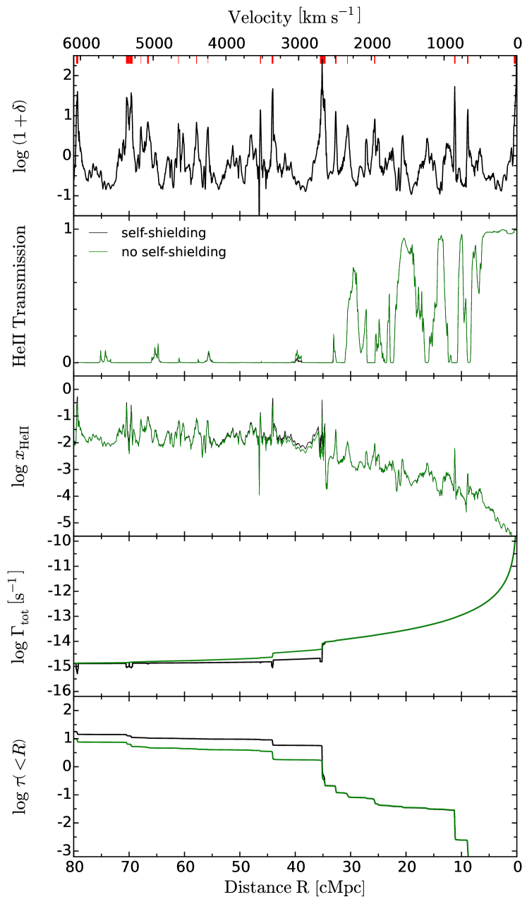
Figure 17.— Impact of Lyman Limit Systems on the proximity zone. From top to bottom panels show: distribution of the overdensities (all locations of He II-LLS are marked by the red ticks on top), transmission in He II, evolution of the He II fraction $x_{\rm HeII}$, total photoionization rate $\Gamma_{\rm tot}$ and the Lyman continuum optical depth $\tau\left(<R\right)$.

Note that ignoring LLSs can lead to inaccurate results for three different reasons: 1) the initial He II fractions are not correct in the LLS pixels because the pixels are initialized under the assumption that they are optically thin, and the initial He II fractions in these pixels are thus set too low. These self-shielding pixels should have very high He II fractions, but instead they start out highly doubly ionized and thus reach their equilibrium ionization state too soon; 2) the total photoionization rate $\Gamma_{\rm tot}$ in the He II-LLS pixels is incorrect because the UVB is not attenuated, hence their $t_{\rm eq}$ are too short, and they thus evolve away from their (incorrect) initial state too fast; 3) these two effects result in incorrect He II fractions at various He II-LLS locations along the skewer, which then implies that the amount of attenuation between any location and the quasar is incorrectly modeled, the photoionization rate $\Gamma_{\rm tot}$ is overestimated everywhere, and thus evolution of the He II fractions in the proximity zone will proceed too quickly.

Now first consider locations very close to the quasar, i.e., $R\ll R_{\rm bkg}$, such that the quasar dominates over the background. For these locations the presence of He II-LLSs make no difference. Referring to the three reasons described above, we can see that this is true because: 1) very near the quasar $t_{\rm eq}(R)\sim 10^{4}-10^{5}\,{\rm yr}$ and thus for the typical quasar lifetimes we consider $t_{\rm eq}\ll t_{\rm Q}$ and the He II fraction has already reached its equilibrium value and has no memory of the incorrect LLS initial conditions; 2) the quasar completely dominates over the UVB, so incorrectly attenuating the UVB changes $t_{\rm eq}=\Gamma_{\rm tot}^{-1}$ negligibly; 3) given that 1) and 2) will be even more true closer to the quasar, the attenuation is correctly modeled, and the He II fractions with and without He II-LLSs are essentially the same. Examining Figure 17, we see that for $R<30$ cMpc, where the quasar radiation completely dominates over the He II ionizing background, all parameters are indistinguishable with and without self-shielding.

At distances $R>30$  cMpc one reaches the regime where the He II background becomes comparable to the photoionization rate of the quasar and LLSs become important. According to the three criteria we used before this happens because: 1) for typical values of quasar lifetimes that we consider $t_{\rm eq}\geq t_{\rm Q}$ and thus $x_{\rm HeII}$ can still be out of equilibrium at $t\sim t_{\rm Q}$. Consequently, setting the initial He II fraction correctly based on the attenuated background radiation field $\Gamma_{\rm HeII}^{\rm bkg}$ is important. If LLS attenuation is ignored, the initial $x_{\rm HeII}$ are too low and are underestimated at the end of each time-step; 2) because at these radii $\Gamma_{\rm HeII}^{\rm bkg}\sim\Gamma_{\rm QSO}$ the equilibration time becomes strongly dependent on $\Gamma_{\rm HeII}^{\rm bkg}$ and it will be too short if the UVB is not attenuated properly, thus the rate of the gas evolution will be incorrect; 3) the result is the lack of attenuation in the overdense pixels, which leads to the too quick evolution of a proximity zone. One can see this effect in Figure 17 at $R>30$  cMpc. The photoionization rate in the no self-shielding case (green) is clearly overestimated in the He II-LLSs, where $x_{\rm HeII}$ is lower than in the self-shielding case (black).

Finally, at distances $R>60$  cMpc, the total photoionization rate $\Gamma_{\rm tot}$ is totally dominated by the UV background and the quasar radiation $\Gamma_{\rm QSO}$ has a very weak effect on the IGM. But at this point the treatment of He II-LLSs is unimportant for predicting the transmitted flux because essentially all of the transmission in the He II Ly$\alpha$ forest comes from the underdense regions and the He II-LLSs are always line black.

Ultimately, He II-LLSs do not change the results dramatically neither in the inner part of the proximity zone, nor at larger distances ($R>30$ cMpc) where they have the biggest effect on the photoionization rate and thus He II fraction. The reason is that in both models the optical depth $\tau\left(<R\right)$ becomes larger than unity at $R\sim 30$ cMpc and the resulting attenuation ${\rm e}^{-\tau}$ is effectively the same with or without self-shielding. Therefore, despite some differences at large distances, inside the proximity zone of the quasar, where the ionizations are dominated by the quasar, the effect of self-shielding in LLSs on the ionizing background radiation field is negligible.

In addition, high column density H I absorption line systems ($N_{\rm HI}\gtrsim 10^{-17}{\rm cm^{-2}}$, i.e. H I LLSs) might also impact our radiative transfer calculations. Although these dense clouds are only rarely encountered in the ambient IGM, they are preferentially clustered around quasars (Hennawi et al., 2006; Hennawi & Prochaska, 2007; Prochaska et al., 2013a, 2015), and the photoevaporation of such systems may slow down the propagation of the ionization fronts and, consequently, change the structure of He II transmission profiles. In order to investigate the impact of these systems on our results, we artificially increased the overdensity of pixels at $R\lesssim 150$ ckpc radius from the location of the quasar halo by a factor of 5. We then performed our radiative transfer calculations again and found no significant differences in the resulting He II transmission. However, we note that in order to fully explore the effect of high column density H I systems one should do a coupled radiative transfer calculation of H I, He I and He II.

Appendix C Appendix C: He II ionizing radiation from recombinations

The recombinations to the ground state of He II produce additional He II ionizing radiation, that can affect the evolution of the He II fraction and subsequently change the transmission profile in the He II proximity zone. In reality calculation of this radiation is a $3$D problem that can not be simply addressed with our $1$D radiative transfer algorithm. In addition, introducing this radiation in our radiative transfer algorithm would effectively make each cell also a source of ionizing radiation and, therefore, would complicate the calculations. In what follows, we estimate the importance of recombination radiation using a simple analytical toy model and argue that it can be safely neglected.

Consider a spherically symmetric region around the quasar of size equal to the radius of the ionization front $R_{\rm IF}$ (see eqn. 15). For the purpose of this calculations let us assume that He II ionizing photons are produced only from the recombinations of helium ions and free electrons inside this region. We assume further that the distribution of the gas density and temperature ($T=10^{4}$ K) are homogeneous inside the region with an average He II fraction $x_{\rm HeII}=0.02$, and that all recombination radiation is emitted only at a single frequency $\nu_{\rm th}$ corresponding to the He II ionization threshold of $4$ Ryd. A remote observer tracks the evolution of the radiation field inside the region only along a $1$D line-of-sight towards the center of the region.

Using the equation of radiative transfer we can estimate the monochromatic intensity $I_{\nu}$ of the recombination radiation at any location $R$ along the line-of-sight coming from the location $R^{\prime}$ inside the spherical region as

$$I_{\nu}=\int_{0}^{s\left(R^{\prime}-R\right)}j_{\nu}e^{-\tau_{\rm s}}{\rm d}s$$ (C1)

where $\tau_{\rm s}=\int_{0}^{s\left(R^{\prime}-R\right)}N_{\rm HeII}\sigma_{\nu}{\rm d}s$ is the optical depth in the IGM along the direction $s\left(R^{\prime}-R\right)$ connecting points $R^{\prime}$ and $R$. This distance $s\left(R^{\prime}-R\right)$ can be expressed through the viewing angle $\theta$ ($0<\theta<\pi$) between the radial direction to $R^{\prime}$ and the line-of-sight as

$$s\left(R^{\prime}-R\right)^{2}=R^{2}+R^{\prime 2}-2RR^{\prime}\cos(\theta)$$ (C2)

We choose to align our $z$-axis with the direction of R and hence $\theta$ is the usual polar angle in spherical coordinates. The free-bound emissivity $j_{\nu}$ is given by

$$j_{\nu}=\frac{h^{4}\nu^{3}}{(2\pi m_{\rm e}kT)^{3/2}c^{2}}e^{\frac{-h(\nu-\nu_{\rm th})}{k_{\rm B}T}}n_{\rm e}n_{\rm HeIII}\sigma_{\nu}\left(\nu\right)$$ (C3)

where $n_{\rm e}$ and $n_{\rm HeIII}$ are the densities of electrons and ions, respectively.

Combining eqn. (C1) and eqn. (C3) the intensity of the recombination radiation can be written as

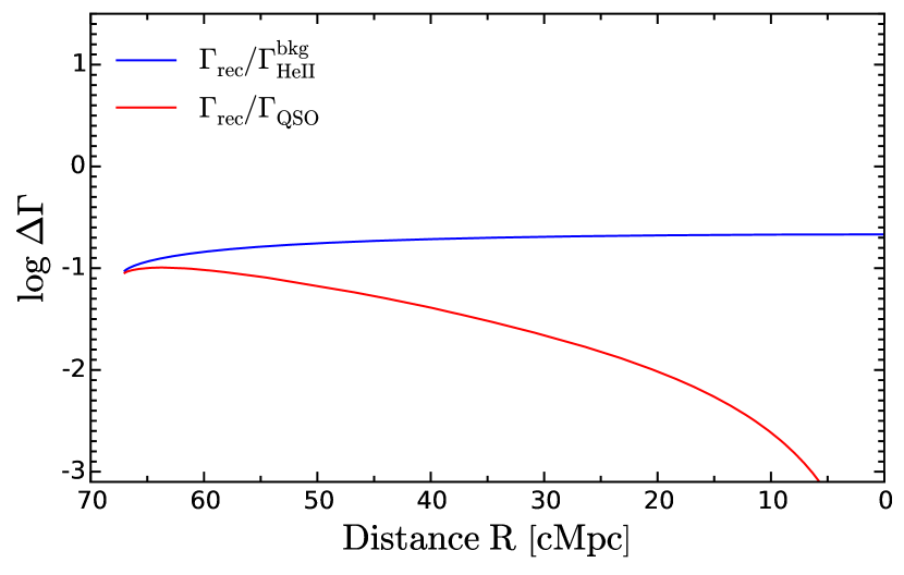
Figure 18.— Comparison between He II recombination radiation photoionization rate $\Gamma_{\rm rec}$ and quasar photoionization rate $\Gamma_{\rm QSO}$ (red curve) and He II ionizing background $\Gamma_{\rm HeII}^{\rm bkg}=10^{-14.9}{\rm s^{-1}}$ (blue curve) for mean He II fraction $\langle x_{\rm HeII}\rangle=0.02$.

$$I_{\nu}\left(\theta\right)=\int_{0}^{s\left(R^{\prime}-R\right)}\frac{h^{4}\nu^{3}\sigma_{\nu}\left(\nu\right)n_{\rm e}n_{\rm HeIII}}{(2\pi m_{\rm e}k_{\rm B}T)^{3/2}c^{2}}e^{\frac{-h(\nu-\nu_{\rm th})}{k_{\rm B}T}}e^{-\tau_{s}}{\rm d}s$$ (C4)

Integrating over the solid angle $\Omega$ we obtain the mean azimuthally symmetric intensity of the recombination radiation $4\pi J_{\nu}$ at location $R$ along the line-of-sight

$$4\pi J_{\nu}=\int I_{\nu}{\rm d}\Omega=2\pi\int_{0}^{\pi}I_{\nu}\left(\theta\right)\sin{\theta}{\rm d}\theta$$ (C5)

Lastly, given eqn. (C5) for the mean intensity $4\pi J_{\nu}$ we calculate the He II photoionization rate due to recombinations $\Gamma_{\rm rec}$ as

$$\Gamma_{\rm rec}=\int_{\nu_{\rm th}}^{2\nu_{\rm th}}\frac{4\pi J_{\nu}}{h_{\rm P}\nu}\sigma_{\nu}\left(\nu\right){\rm d}\nu$$ (C6)

Recall, that we approximated the recombination radiation as being propagated with a single frequency corresponding to $4$ Ryd. However, this will make it impossible to calculate the frequency-averaged photoionization rate and we, therefore, assume a narrow finite frequency interval $\nu_{\rm th}\leq\nu\leq 2\nu_{\rm th}$ in order to calculate the integral in eqn. (C6).

We compare $\Gamma_{\rm rec}$ to the values of quasar photoionization rate $\Gamma_{\rm QSO}$ and He II ionizing background $\Gamma_{\rm HeII}^{\rm bkg}=10^{-14.9}{\rm s^{-1}}$ taken from our fiducial model with quasar lifetime $t_{\rm Q}=10$ Myr and quasar photon production rate $Q_{\rm 4Ry}=10^{56.1}{\rm s^{-1}}$. The location of the ionization front is this model is approximately $R_{\rm IF}\simeq 67$ cMpc, we thus use this value as a boarder of the region where the recombination radiation is calculated. The results are shown in Figure 18. The blue curve shows the ratio of the He II photoionization rates due to recombinations $\Gamma_{\rm rec}$ and the He II background $\Gamma_{\rm HeII}^{\rm bkg}$. This ratio stays nearly constant throughout the region we consider, with $\Gamma_{\rm rec}$ being $\simeq 10-30\%$ of the $\Gamma_{\rm HeII}^{\rm bkg}$. Not only do recombinations constitute a minor correction to the background, but because $\Gamma_{\rm rec}$ does not vary significantly with distance $R$, it could also be effectively absorbed into the background and thought of as a small correction to it. At the same time, the red curve shows the ratio between $\Gamma_{\rm rec}$ and quasar photoionization rate $\Gamma_{\rm QSO}$. It is clear that the quasar photoionization rate dominants at all distances $R$ from the quasar, making the contribution of recombination radiation to the total radiation field in the He II proximity region essentially negligible.

Although our analtyical estimate of $\Gamma_{\rm rec}$ is admittedly rather crude, according to Figure 18 including recombination radiation in our calculation will not significantly change the results of our $1$D radiative transfer.

Appendix D Appendix D: Generating He II Skewers

We calculate He II spectra along each of the skewers drawn from the SPH simulations following the procedure described in Theuns et al. (1998). We use densities and velocities of the SPH particles at each pixel, combined with the He II fraction and temperature resulting from our radiative transfer calculation to compute the observed flux $F\left(v\right)=e^{-\tau_{\rm HeII}\left(v\right)}$, with the He II optical depth $\tau_{\rm HeII}\left(v\right)$ of the pixel given by

$$\begin{split}\tau_{\rm HeII}\left(v\right)=\frac{\sigma_{\alpha}c}{\sqrt{\pi V}}n_{\rm He}x_{\rm HeII}\left(1+\delta\right)\frac{\Delta R}{1+z}\\ \times{\rm exp}\left(-\left[\frac{v-v_{H}}{V}\right]^{2}\right)\end{split}$$ (D1)

where $V^{2}=2k_{\rm B}T/m_{\rm He}$ is the Doppler width of helium with mass $m_{\rm He}$, $c$ is the speed of light, $T$ is the temperature inside the cell, $n_{\rm He}x_{\rm HeII}$ is the density of He II, $\Delta R$ is the pixel width, $\sigma_{\rm HeII}$ is He II Ly$\alpha$ cross-section, and the term ${v_{\rm H}}$ describes the combination of Hubble and peculiar velocities.

We similarly compute the H I Ly$\alpha$ optical depth. Hydrogen gas is also considered optically thin to the ionizing radiation and analogously to helium, we introduce an H I ionizing background photoionization rate $\Gamma_{\rm HI}^{\rm bkg}$ to mimic the influence of other sources in the Universe, with a value of $\Gamma_{\rm HI}^{\rm bkg}=1\times 10^{-12}{\rm s^{-1}}$ chosen to match the mean transmitted flux at $z\simeq 3.1$ in agreement with recent measurements by Becker et al. (2013).

References

- Abel & Haehnelt (1999) Abel, T., & Haehnelt, M. G. 1999, ApJ, 520, L13
- Adelberger & Steidel (2005) Adelberger, K. L., & Steidel, C. C. 2005, ApJ, 630, 50
- Anderson et al. (1999) Anderson, S. F., Hogan, C. J., Williams, B. F., & Carswell, R. F. 1999, AJ, 117, 56
- Bajtlik et al. (1988) Bajtlik, S., Duncan, R. C., & Ostriker, J. P. 1988, ApJ, 327, 570
- Becker et al. (2013) Becker, G. D., Hewett, P. C., Worseck, G., & Prochaska, J. X. 2013, MNRAS, 430, 2067
- Bolton et al. (2012) Bolton, J. S., Becker, G. D., Raskutti, S., et al. 2012, MNRAS, 419, 2880
- Bolton & Haehnelt (2007a) Bolton, J. S., & Haehnelt, M. G. 2007a, MNRAS, 374, 493
- Bolton & Haehnelt (2007b) —. 2007b, MNRAS, 381, L35
- Borisova et al. (2015) Borisova, E., Lilly, S. J., Cantalupo, S., et al. 2015, ArXiv e-prints, arXiv:1510.00029
- Boroson (2005) Boroson, T. 2005, AJ, 130, 381
- Cantalupo et al. (2014) Cantalupo, S., Arrigoni-Battaia, F., Prochaska, J. X., Hennawi, J. F., & Madau, P. 2014, Nature, 506, 63
- Carilli & Walter (2013) Carilli, C. L., & Walter, F. 2013, ARA&A, 51, 105
- Carilli et al. (2010) Carilli, C. L., Wang, R., Fan, X., et al. 2010, ApJ, 714, 834
- Carswell et al. (1982) Carswell, R. F., Whelan, J. A. J., Smith, M. G., Boksenberg, A., & Tytler, D. 1982, MNRAS, 198, 91
- Cen & Haiman (2000) Cen, R., & Haiman, Z. 2000, ApJ, 542, L75
- Cole & Kaiser (1989) Cole, S., & Kaiser, N. 1989, MNRAS, 237, 1127
- Compostella et al. (2013) Compostella, M., Cantalupo, S., & Porciani, C. 2013, MNRAS, 435, 3169
- Conroy & White (2013) Conroy, C., & White, M. 2013, ApJ, 762, 70
- Croom et al. (2005) Croom, S. M., Boyle, B. J., Shanks, T., et al. 2005, MNRAS, 356, 415
- Davies et al. (2014) Davies, F. B., Furlanetto, S. R., & McQuinn, M. 2014, ArXiv e-prints, arXiv:1409.0855
- Davis et al. (1985) Davis, M., Efstathiou, G., Frenk, C. S., & White, S. D. M. 1985, ApJ, 292, 371
- Fan et al. (2002) Fan, X., Narayanan, V. K., Strauss, M. A., et al. 2002, in Lighthouses of the Universe: The Most Luminous Celestial Objects and Their Use for Cosmology, ed. M. Gilfanov, R. Sunyeav, & E. Churazov, 309
- Fan et al. (2006) Fan, X., Strauss, M. A., Becker, R. H., et al. 2006, AJ, 132, 117
- Faucher-Giguère et al. (2008) Faucher-Giguère, C.-A., Lidz, A., Zaldarriaga, M., & Hernquist, L. 2008, ApJ, 673, 39
- Fechner et al. (2004) Fechner, C., Baade, R., & Reimers, D. 2004, A&A, 418, 857
- Furlanetto & Lidz (2011) Furlanetto, S. R., & Lidz, A. 2011, ApJ, 735, 117
- Gallerani et al. (2008) Gallerani, S., Ferrara, A., Fan, X., & Choudhury, T. R. 2008, MNRAS, 386, 359
- Gonçalves et al. (2008) Gonçalves, T. S., Steidel, C. C., & Pettini, M. 2008, ApJ, 676, 816
- Goodman (2003) Goodman, J. 2003, MNRAS, 339, 937
- Gunn & Peterson (1965) Gunn, J. E., & Peterson, B. A. 1965, ApJ, 142, 1633
- Haardt & Madau (2012) Haardt, F., & Madau, P. 2012, ApJ, 746, 125
- Haiman & Cen (2001) Haiman, Z., & Cen, R. 2001, in Astronomical Society of the Pacific Conference Series, Vol. 222, The Physics of Galaxy Formation, ed. M. Umemura & H. Susa, 101
- Haiman & Hui (2001) Haiman, Z., & Hui, L. 2001, ApJ, 547, 27
- Heap et al. (2000) Heap, S. R., Williger, G. M., Smette, A., et al. 2000, ApJ, 534, 69
- Hennawi & Prochaska (2007) Hennawi, J. F., & Prochaska, J. X. 2007, ApJ, 655, 735
- Hennawi & Prochaska (2013) —. 2013, ApJ, 766, 58
- Hennawi et al. (2015) Hennawi, J. F., Prochaska, J. X., Cantalupo, S., & Arrigoni-Battaia, F. 2015, Science, 348, 779
- Hennawi et al. (2006) Hennawi, J. F., Prochaska, J. X., Burles, S., et al. 2006, ApJ, 651, 61
- Hogan et al. (1997) Hogan, C. J., Anderson, S. F., & Rugers, M. H. 1997, AJ, 113, 1495
- Hopkins et al. (2008) Hopkins, P. F., Hernquist, L., Cox, T. J., & Kereš, D. 2008, ApJS, 175, 356
- Hopkins et al. (2006) Hopkins, P. F., Hernquist, L., Cox, T. J., Robertson, B., & Springel, V. 2006, ApJS, 163, 50
- Hopkins et al. (2005) Hopkins, P. F., Hernquist, L., Martini, P., et al. 2005, ApJ, 625, L71
- Hopkins & Quataert (2010) Hopkins, P. F., & Quataert, E. 2010, MNRAS, 407, 1529
- Jakobsen et al. (2003) Jakobsen, P., Jansen, R. A., Wagner, S., & Reimers, D. 2003, A&A, 397, 891
- Kirkman & Tytler (2008) Kirkman, D., & Tytler, D. 2008, MNRAS, 391, 1457
- Kormendy & Ho (2013) Kormendy, J., & Ho, L. C. 2013, ARA&A, 51, 511
- Kormendy & Richstone (1995) Kormendy, J., & Richstone, D. 1995, ARA&A, 33, 581
- Larson et al. (2011) Larson, D., Dunkley, J., Hinshaw, G., et al. 2011, ApJS, 192, 16
- Lidz et al. (2007) Lidz, A., McQuinn, M., Zaldarriaga, M., Hernquist, L., & Dutta, S. 2007, ApJ, 670, 39
- Lusso et al. (2015) Lusso, E., Worseck, G., Hennawi, J. F., et al. 2015, ArXiv e-prints, arXiv:1503.02075
- Madau & Meiksin (1994) Madau, P., & Meiksin, A. 1994, ApJ, 433, L53
- Madau & Rees (2000) Madau, P., & Rees, M. J. 2000, ApJ, 542, L69
- Martini (2004) Martini, P. 2004, Coevolution of Black Holes and Galaxies, 169
- Martini & Weinberg (2001) Martini, P., & Weinberg, D. H. 2001, ApJ, 547, 12
- Maselli et al. (2007) Maselli, A., Gallerani, S., Ferrara, A., & Choudhury, T. R. 2007, MNRAS, 376, L34
- McQuinn (2009b) McQuinn, M. 2009b, ApJ, 704, L89
- McQuinn et al. (2009a) McQuinn, M., Lidz, A., Zaldarriaga, M., et al. 2009a, ApJ, 694, 842
- McQuinn & Switzer (2010) McQuinn, M., & Switzer, E. R. 2010, MNRAS, 408, 1945
- McQuinn & Worseck (2014) McQuinn, M., & Worseck, G. 2014, MNRAS, 440, 2406
- Meiksin et al. (2010) Meiksin, A., Tittley, E. R., & Brown, C. K. 2010, MNRAS, 401, 77
- Mellema et al. (2006) Mellema, G., Iliev, I. T., Alvarez, M. A., & Shapiro, P. R. 2006, NA, 11, 374
- Mesinger & Haiman (2004) Mesinger, A., & Haiman, Z. 2004, ApJ, 611, L69
- Miralda-Escudé et al. (2000) Miralda-Escudé, J., Haehnelt, M., & Rees, M. J. 2000, ApJ, 530, 1
- Prochaska et al. (2013a) Prochaska, J. X., Hennawi, J. F., & Simcoe, R. A. 2013a, ApJ, 762, L19
- Prochaska et al. (2015) Prochaska, J. X., O’Meara, J. M., Fumagalli, M., Bernstein, R. A., & Burles, S. M. 2015, ApJS, 221, 2
- Prochaska et al. (2013b) Prochaska, J. X., Hennawi, J. F., Lee, K.-G., et al. 2013b, ApJ, 776, 136
- Schawinski et al. (2015) Schawinski, K., Koss, M., Berney, S., & Sartori, L. F. 2015, MNRAS, 451, 2517
- Schawinski et al. (2010) Schawinski, K., Evans, D. A., Virani, S., et al. 2010, ApJ, 724, L30
- Shapiro et al. (2006) Shapiro, P. R., Iliev, I. T., Alvarez, M. A., & Scannapieco, E. 2006, ApJ, 648, 922
- Shen et al. (2009) Shen, Y., Strauss, M. A., Ross, N. P., et al. 2009, ApJ, 697, 1656
- Shen et al. (2011) Shen, Y., Richards, G. T., Strauss, M. A., et al. 2011, ApJS, 194, 45
- Shull et al. (2010) Shull, J. M., France, K., Danforth, C. W., Smith, B., & Tumlinson, J. 2010, ApJ, 722, 1312
- Shull et al. (2012) Shull, J. M., Stevans, M., & Danforth, C. W. 2012, ApJ, 752, 162
- Soltan (1982) Soltan, A. 1982, MNRAS, 200, 115
- Springel (2005c) Springel, V. 2005c, MNRAS, 364, 1105
- Springel et al. (2005a) Springel, V., Di Matteo, T., & Hernquist, L. 2005a, ApJ, 620, L79
- Springel et al. (2005b) —. 2005b, MNRAS, 361, 776
- Syphers et al. (2012) Syphers, D., Anderson, S. F., Zheng, W., et al. 2012, AJ, 143, 100
- Syphers & Shull (2014) Syphers, D., & Shull, J. M. 2014, ApJ, 784, 42
- Telfer et al. (2002) Telfer, R. C., Zheng, W., Kriss, G. A., & Davidsen, A. F. 2002, ApJ, 565, 773
- Theuns et al. (1998) Theuns, T., Leonard, A., Efstathiou, G., Pearce, F. R., & Thomas, P. A. 1998, MNRAS, 301, 478
- Trainor & Steidel (2013) Trainor, R., & Steidel, C. C. 2013, ApJ, 775, L3
- White et al. (2012) White, M., Myers, A. D., Ross, N. P., et al. 2012, MNRAS, 424, 933
- White et al. (2003) White, R. L., Becker, R. H., Fan, X., & Strauss, M. A. 2003, AJ, 126, 1
- Worseck et al. (2007) Worseck, G., Fechner, C., Wisotzki, L., & Dall’Aglio, A. 2007, A&A, 473, 805
- Worseck et al. (2014) Worseck, G., Prochaska, J. X., Hennawi, J. F., & McQuinn, M. 2014, ArXiv e-prints, arXiv:1405.7405
- Worseck & Wisotzki (2006) Worseck, G., & Wisotzki, L. 2006, A&A, 450, 495
- Worseck et al. (2011) Worseck, G., Prochaska, J. X., McQuinn, M., et al. 2011, ApJ, 733, L24
- Wyithe et al. (2008) Wyithe, J. S. B., Bolton, J. S., & Haehnelt, M. G. 2008, MNRAS, 383, 691
- Wyithe & Loeb (2003) Wyithe, J. S. B., & Loeb, A. 2003, ApJ, 595, 614
- Yu & Lu (2004) Yu, Q., & Lu, Y. 2004, ApJ, 602, 603
- Yu & Tremaine (2002) Yu, Q., & Tremaine, S. 2002, MNRAS, 335, 965
- Zheng et al. (2015) Zheng, W., Syphers, D., Meiksin, A., et al. 2015, ApJ, 806, 142