Solitons and vortices in nonlinear potential wells

Abstract

We consider self-trapping of topological modes governed by the one- and two-dimensional (1D and 2D) nonlinear-Schrödinger/Gross-Pitaevskii equation with effective single- and double-well (DW) nonlinear potentials induced by spatial modulation of the local strength of the self-defocusing nonlinearity. This setting, which may be implemented in optics and Bose-Einstein condensates, aims to extend previous studies, which dealt with single-well nonlinear potentials. In the 1D setting, we find several types of symmetric, asymmetric and antisymmetric states, focusing on scenarios of the spontaneous symmetry breaking. The single-well model is extended by including rocking motion of the well, which gives rise to Rabi oscillations between the fundamental and dipole modes. Analysis of the 2D single-well setting gives rise to stable modes in the form of ordinary dipoles, vortex-antivortex dipoles (VADs), and vortex triangles (VTs), which may be considered as produced by spontaneous breaking of the axial symmetry. The consideration of the DW configuration in 2D reveals diverse types of modes built of components trapped in the two wells, which may be fundamental states and vortices with topological charges $m=1$ and $2$, as well as VADs (with $m=0$) and VTs (with $m=2$).

I Introduction and the model

It is commonly known that in spaces of different dimension, $D$, bright solitons of scalar complex field $\phi$ may be supported by balance between the focusing nonlinearity and diffraction Agrawal . The solitons created by focusing term $|\phi|^{2m}\phi$ in the underlying nonlinear Schrödinger/Gross-Pitaevskii equation (NLSE/GPE) are unstable in the case when the same setting gives rise to the collapse, i.e., at $mD\geq 2$, according to the Talanov’s criterion Talanov . In particular, the Townes’ solitons Townes , which form degenerate families with the norm that does not depend on the propagation constant, are destabilized by the critical collapse (corresponding to $mD=2$) in the 2D space with the cubic nonlinearity, $m=1$ Berge' , and in the 1D space with the quintic self-focusing, $m=2$ Mario .

In the absence of linear trapping potentials, an effective nonlinear potential (alias pseudopotential pseudo ) for optical waves in photonic media, and for matter waves in a Bose-Einstein condensate (BEC) BEC can be induced by the spatial modulation of the local strength of the cubic nonlinearity, accounted for by coefficient $\sigma(\mathbf{r})$ RMP :

$$i\psi_{z}=-\frac{1}{2}\nabla^{2}\psi+\sigma(\mathbf{r})|\psi|^{2}\psi,$$ (1)

the respective Hamiltonian being

$$H=\frac{1}{2}\int\int\left[\left|\nabla\psi\right|^{2}+\sigma(x)|\phi(x)|^{4}\right]dx.$$ (2)

In optics, $\psi$ is the scaled amplitude of the guided electromagnetic field, $z$ is the propagation distance and the set of transverse coordinates is $\mathbf{r}=(x,y)$ or $x$, in the 1D and 2D settings, respectively. In terms of the GPE, $z$ is the scaled time, and the scattering length, which is proportional to $\sigma(\mathbf{r})$ in Eq. (1), can be modified by means of the Feshbach resonance in external magnetic or optical fields FR-Randy -FR-Tom . The spatial modulation of the scattering length in atomic condensates was experimentally demonstrated on the submicron scale experiment-inhom-Feshbach . The necessary spatial profile may be also induced as an averaged spatial pattern “painted” by a fast moving laser beam painting , or by an optical-flux lattice Cooper . Another approach makes use of an appropriate magnetic lattice, into which the condensate is loaded magn-latt , or of magnetic-field concentrators concentrator . In optics, the modulation of the nonlinearity strength can be achieved by means of inhomogeneous doping of the waveguide with nonlinearity-enhancing impurities Kip . Alternatively, one can use a uniform dopant density, onto which an external field imposes an inhomogeneous distribution of detuning from the respective two-photon resonance.

The nonlinear potential induced by the modulation of the self-focusing nonlinearity, which corresponds to $\sigma(\mathbf{r})<0$ in Eq. (1), can readily support stable solitons in the 1D geometry, as has been demonstrated in various settings 1D-attr ; Thawatchai . On the other hand, in the 2D geometry, stable fundamental solitons can be maintained only by modulation profiles with sharp edges, all vortex solitons being unstable 2D-attr ; 2D-Thawatchai ; RMP .

Recently, an alternative scheme was theoretically elaborated, based on the defocusing-nonlinearity strength growing at $r\rightarrow\infty$ at any rate exceeding $r^{D}$ Barcelona -SR . This scheme secures stable self-trapping of a great variety of fundamental and higher-order solitons, including solitary vortices Barcelona ; Barcelona2 ; SR , and complex 3D modes, such as soliton gyroscopes gyroscope , vortex-antivortex hybrids hybrid , and “hopfions” (vortex tori with intrinsic twist) Yasha . Moreover, the scheme was extended for discrete solitons discrete , quantum solitons in the Bose-Hubbard model LucaLuca , and 1D and 2SD settings with the spatially modulated long-range dipole-dipole repulsive interactions Raymond .

Stationary solutions to Eq. (1) are looked for as

$$\psi(\mathbf{r},z)=\phi(\mathbf{r})e^{i\mu z},$$ (3)

where $\mu$ determines the propagation constant, in terms of photonic models, or the chemical potential, $-\mu$, in BEC, and stationary wave function $\phi$ obeys equation

$$\mu\phi=\frac{1}{2}\nabla^{2}\phi+\sigma(\mathbf{r})|\phi|^{2}\phi.$$ (4)

Self-trapped solutions supported by the system are characterized by the norm (energy flow), defined as

$$N=\int\left|\phi(\mathbf{r})\right|^{2}d\mathbf{r}.$$ (5)

We aim to consider two types of nonlinearity-modulation profiles, in the 1D and 2D geometries alike. The first corresponds to the isotropic single-well setting, with the steep anti-Gaussian shape, which was introduced in Ref. Barcelona2 :

$$\sigma(\mathbf{r})=\exp\left(\alpha r^{2}\right),$$ (6)

with constant $\alpha>0$ which determines the width of the well, $\sim\alpha^{-1/2}$. Another version of the single-well profile, including a pre-exponential factor, was also considered in Ref. Barcelona2 :

$$\sigma(\mathbf{r})=\left(\sigma_{0}+\frac{\sigma_{2}}{2}r^{2}\right)\exp\left(\alpha r^{2}\right).$$ (7)

The main subject of the present work is an anisotropic double-well (DW) profile, whose 2D form can be defined as a natural extension of its single-well counterpart, possibly with the addition of a pre-exponential factor:

$$\sigma(\mathbf{r})=\left\{\sigma_{0}+\frac{\sigma_{2}}{2}\left[(|x|-x_{0})^{2}+y^{2}\right]\right\}\exp\left\{\alpha\left[(|x|-\beta x_{0})^{2}+y^{2}\right]\right\}$$ (8)

[cf. Eq. (7)], with constants $\sigma_{0,2}\geq 0$, and $x_{0}\geq 0$, where $x=\pm x_{0}$ are positions of centers of the two wells. Different types of the DW structure correspond to $\beta=1$ and $\beta=0$ in Eq. (8) (in the latter case, the bottom of each well is shifted from $x=\pm x_{0}$ towards $x=0$). A particular DW profile corresponds to $\sigma_{0}=1,\sigma_{2}=0,\beta=1$ in Eq. (8) [cf. Eq. (6) for the single well]:

$$\sigma(\mathbf{r})=\exp\left\{\alpha\left[(|x|-\beta x_{0})^{2}+y^{2}\right]\right\}.$$ (9)

The 1D counterpart of the DW setting based on Eq. (9) is considered below too.

It is commonly known that the ground state generated by the linear Schrödinger equation with a DW potential is always symmetric, with respect to the two potential wells LL . The interplay of the linear DW potentials with uniform self-focusing nonlinearities in models based on the NLSE/GPE gives rise to the fundamental effect of the spontaneous symmetry breaking (SSB) book ; NewsViews . In its simplest manifestation, the SSB implies that the probability to find the particle in one well of the DW potential is larger than in the other. This also means that another principle of quantum mechanics, according to which the ground state cannot be degenerate, is no longer valid in the nonlinear systems, as the SSB creates a degenerate pair of two mutually symmetric ground states, with the maximum of the wave function trapped in either potential well. While the same system admits a symmetric state coexisting with the asymmetric ones, it no longer represents the ground state above the SSB point, being, unstable against symmetry-breaking perturbations. In systems with the defocusing nonlinearity, the ground state remains symmetric and stable, while the SSB manifests itself in the form of the spontaneous breaking of the spatial antisymmetry of the first excited state.

The SSB was introduced in early works Davies , and then developed in detail in the system modeling the propagation of continuous-wave optical beams in dual-core nonlinear optical fibers Snyder . Depending on the form of the nonlinearity, it gives rise to symmetry-breaking bifurcations of the supercritical (alias forward) or subcritical (backward) type bif . The next step in the studies of the SSB phenomenology in dual-core systems was the detailed consideration of this effect for solitons, described by a system of linearly coupled partial differential NLSEs Wabnitz -Pak . The transition to asymmetric solitons in this system was predicted by means of the variational approximation Pare ; Pak and investigated in a numerical form Akhmed ; Pak . The analysis of the SSB in BEC and other models based on the GPE with the DW potential was initiated in Ref. Milburn , and later extended for bosonic Josephson junctions junction -junction-reviews and matter-wave solitons Warsaw .

Experimentally, the self-trapping of asymmetric states in the BEC of ⁸⁷Rb atoms loaded into the DW potential, as well as Josephson oscillations in the same setting, were reported in Ref. Markus . The SSB of laser beams coupled into an effective transverse DW potential created in a photorefractive medium was demonstrated in Ref. photo . A spontaneously established asymmetric regime of the operation of a symmetrically coupled pair of lasers was reported too lasers .

Here, our main objective is to study the SSB of self-trapped modes supported by effective nonlinear (pseudo)potentials. Previously, some results for such settings were reported in Refs. Thawatchai and China-DW , but the systematic analysis based on the model with the spatially modulated strength of the self-defocusing nonlinearity was not developed. Because we consider the models with the defocusing sign of the nonlinearity, the respective symmetric ground state is always stable and is not subject to the

SSB, as mentioned above. Therefore, we focus on the SSB featured by antisymmetric (dipole) modes, in the form of the spontaneous breaking of their spatial antisymmetry. Another manifestation of the SSB that we address in this work is spontaneous formation of anisotropic patterns in the 2D isotropic single-well configuration, a known example of that in usual models with the uniform nonlinearity being the creation of azimuthons azi .

Localized solutions to the 1D version of the stationary equation (4) are obtained in the numerical form by means of the Newton-Raphson method Yang . Symmetric 1D and 2D modes are also produced in an approximate analytical form by means of the Thomas-Fermi approximation (TFA). The stability was then studied by adding small perturbations to the stationary solutions, $e^{i\mu z}\phi_{s}(x)$, in the form of

$$\psi(x,z)=e^{i\mu z}\left[\phi_{s}(x)+g(x)e^{-i\lambda t}+f^{\ast}(x)e^{i\lambda^{\ast}z}\right],$$ (10)

cf. Eq. (3), where $g(x)$ and $f(x)$ are eigenmodes of the infinitesimal perturbation, $\lambda$ is the corresponding eigenfrequency, which is complex (in particular, imaginary) in the case of instability, and the asterisk stands for the complex conjugation. Substituting the perturbed solution, (10), in Eq. (4) and the subsequent linearization results in the following eigenvalue problem,

$$\left(\begin{array}[]{cc}\hat{L}&\sigma(x)\left(\phi_{s}(x)\right)^{2}\\ -\sigma(x)\left(\phi_{s}(x)\right)^{2}&-\hat{L}\end{array}\right)\left(\begin{array}[]{c}g(x)\\ f(x)\end{array}\right)=\lambda\left(\begin{array}[]{c}g(x)\\ f(x)\end{array}\right),$$ (11)

with $\hat{L}=\mu-(1/2)d^{2}/dx^{2}+2\sigma(x)\left(\phi_{s}(x)\right)^{2}$. This problem can be solved using the basic finite-difference scheme, thus finding the set of eigenfrequencies $\lambda$ and determining the stability of the underlying solution. In addition, direct numerical simulations of initially perturbed solutions are performed by means of the pseudospectral split-step Fourier method, to verify the predicted stability, as well as to explore the evolution of unstable states. The direct simulations are run with absorbers installed at edges of the computation domain. In the 2D setting, stationary solutions are obtained by dint of the modified squared-operator method introduced in Ref. Lakoba (see also book Yang ), and the stability is then investigated primarily through direct simulations.

The rest of the paper is organized as follows. The 1D DW setting and the SSB effect in it are considered in Section II. The dynamics of trapped modes in a single rocking (periodically moving) 1D well is addressed in Section III. Various stable and unstable states trapped in the single- and double-well structures in 2D are considered in Sections IV and V, respectively. The paper is concluded by Section VI.

II The one-dimensional setting

II.1 Basic 1D states: Symmetric, anti-symmetric, and asymmetric solitons

The 1D version of model (4), with the simplest DW modulation profile taken as the 1D variant of Eq. (9),

$$\sigma(x)=\exp\left[\alpha\left(\left(|x|-x_{0}\right)^{2}\right)\right],$$ (12)

gives rise to basic families of symmetric, antisymmetric and asymmetric (antisymmetry-breaking) states. Typical examples of shapes of these three types are presented in Fig. 1, for $\alpha=0.5$, $x_{0}=1$ and $\mu=5$.

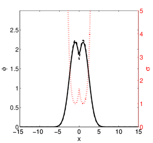
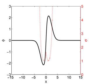
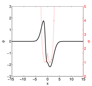
Figure 1: (Color online) Examples of numerically found 1D symmetric (a), antisymmetric (b) and asymmetric (c) states, for $\mu=5$ and the double-well nonlinearity-modulation profile given by Eq. (12) (depicted by the red dotted line), with $\alpha=0.5$ and $x_{0}=1$. The dashed line in (a), which almost overlaps with the numerically generated continuous profile, displays the respective TFA (Thomas-Fermi approximation), as given by Eq. (13).

The symmetric solutions, which represent the ground state of the model (see below), can be analytically approximated  by means of the TFA, which was efficiently applied to the description of ground states in 1D, 2D, and 3D versions of the model with the single-well structure Barcelona -Yasha , Raymond . The TFA neglects the kinetic-energy term (the second-order derivative) in the 1D version of Eq. (4), with $\sigma(x)$ substituted by expression (12):

$$\phi_{\mathrm{TFA}}(x)=\sqrt{\mu}\exp\left[-\left(\alpha/2\right)\left(|x|-x_{0}\right)^{2}\right].$$ (13)

The respective approximation for the norm of the symmetric modes is

$$N_{\mathrm{TFA}}(\mu)=\sqrt{\pi/\alpha}\mu\left[1+\mathrm{erf}\left(\sqrt{\alpha}x_{0}\right)\right],$$ (14)

where $\mathrm{erf}$ is the standard error function. The comparison of the TFA profile with its numerically generated counterpart is displayed in Fig. 1.

The stability investigation was conducted for all the three basic families, by numerically solving the eigenvalue problem based on Eq. (11), at different values of $\mu$ (i.e., different norms $N$), and different values of parameters $x_{0}$ and $\alpha$. It has been found that the symmetric family, which does not undergo any bifurcation, is completely stable.

The antisymmetric solutions are stable for low values of $\mu$ (sufficiently small $N$). Increasing $\mu$, one hits a bifurcation point, above which the antisymmetric state loses its stability and a new asymmetric (antisymmetry-breaking) branch emerges. This asymmetric branch may be stable, at least partially, depending on values of $x_{0}$ and $\alpha$.

Figure 2 demonstrates the stable symmetric branch, as well as the antisymmetric/asymmetric bifurcation scenario, for $x_{0}=1$ and $\alpha=0.5$. As shown in this example, and is true in the general case too, for all values of $x_{0}$ and $\alpha$ examined, the bifurcation is of the supercritical type, which means that the asymmetric solutions are stable immediately after the bifurcation point. Figure 2 shows that bistability exists between the symmetric and antisymmetric modes, and between the symmetric and asymmetric ones, below and above the bifurcation, respectively.

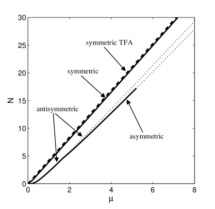
Figure 2: Branches $N(\mu)$ for symmetric, antisymmetric and asymmetric modes trapped in the 1D double-well nonlinear potential, for $x_{0}=1$ and $\alpha=0.5$. Here and in similar figures following below, stable and unstable solutions are indicated by continuous and dotted lines, respectively. The dashed line shows the TFA, as produced by Eq. (14) for the symmetric modes. This analytical approximation readily explains the nearly linear form of $N(\mu)$.

In the case shown in Fig. 2, the asymmetric branch is stable in a limited region, starting from the bifurcation point (at $\mu=1.719$, $N=4.748$) and up to $\mu=5.206$, $N=17.21$. The stability domain strongly depends on $\alpha$, as shown in Fig. 3, which displays stability/instability domains for the asymmetric states in the $\left(\alpha,N\right)$ plane for $x_{0}=1$ [this may be fixed in Eq. (4) by means of obvious rescaling]. In particular, for $\alpha<0.351$ the asymmetric states are stable in their entire existence region.

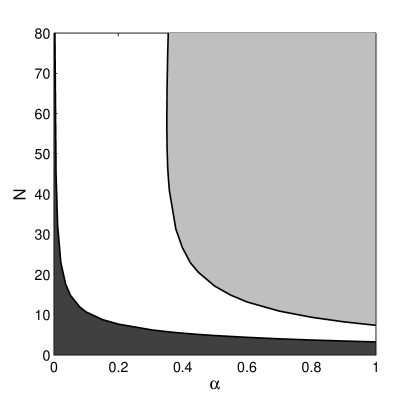
Figure 3: The stability diagram for the 1D asymmetric modes, in the $\left(\alpha,N\right)$ plane, at fixed $x_{0}=1$. Stable solutions exist in the white region. Asymmetric solutions do not exist in the dark area, at the bottom and left side of the diagram (the border between the white and dark regions is the line of the antisymmetry-breaking bifurcation for the antisymmetric branch). Unstable asymmetric solutions exist in the light-gray region.

Direct simulations, for unstable asymmetric states and unstable antisymmetric ones, demonstrate that they develop an oscillatory instability  and eventually converge to stable symmetric modes. The linear stability analysis shows that the instability of asymmetric states (when they are unstable) are accounted for by complex eigenvalues, while the unstable antisymmetric states are characterized by imaginary eigenvalues. With the increase of $\mu$ (i.e., the increase of the norm), the duration of the intermediate oscillatory evolution shrinks, which is related to the fact that the imaginary part of the stability eigenvalues (i.e., the instability growth rate) increases with the norm. Examples of the evolution of unstable asymmetric states are shown in Fig. 4, for $x_{0}=1$, $\alpha=0.5$, and $\mu=6.5$ or $15$. In these examples, the interval of the oscillatory behavior shrinks from $50<z<275$ at $\mu=6.5$ ($N=22.12$), to virtually no oscillations at $\mu=15$ ($N=55.26$). Similar results were obtained for unstable antisymmetric solutions, see Fig. 5. In this case, the interval of the oscillations shrinks from $20<z<215$ at $\mu=6.5$ ($N=23.34$) to $10<z<75$ at $\mu=15$ ($N=57.57$).

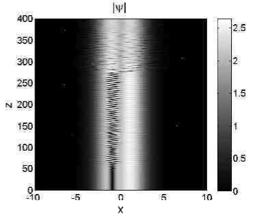
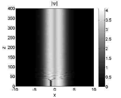
Figure 4: (Color online) The evolution of unstable 1D asymmetric states, at $x_{0}=1$, $\alpha=0.5$, into stable symmetric modes. (a) A conspicuous interval of the oscillatory instability is observed at relatively low values of $\mu$ (or $N$), here for $\mu=6.5$. (b) For large $\mu$ (here, for $\mu=15$). the transition to the symmetric state is much faster.

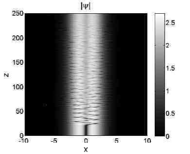
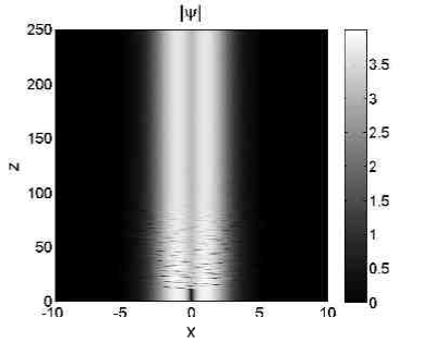
Figure 5: (Color online) The evolution of unstable 1D antisymmetric states into stable symmetric ones, at $x_{0}=1$ and $\alpha=0.5$: (a) $\mu=6.5$; (b) $\mu=15$.

In fact, the dynamics observed in Figs. 4(a) and 5(a) may be regarded as a manifestation of Josephson oscillations in the underlying bosonic coupler junction ; Markus ; junction2 ; junction-reviews .

II.2 Novel 1D modes: excited symmetric and composite asymmetric modes

The numerical analysis has revealed several new types of 1D states. One of them is the first excited symmetric state, which is shown in Fig. 6 for $x_{0}=1$, $\mu=5$ and $\alpha=0.5$. The classification of this state is based on the consideration of its energy, see below. This solution is actually a composition of two mutually reversed dipole states, centered in each well (this is better seen when the wells are set farther apart). The stability diagram for this type of the solutions is presented in Fig. 6. Note that (completely stable) excited symmetric states with two nodes ($k=2$) were also found in the model of the same type, but with a single-well shape of the local-nonlinearity modulation Barcelona2 .

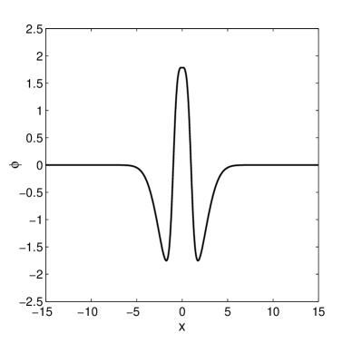
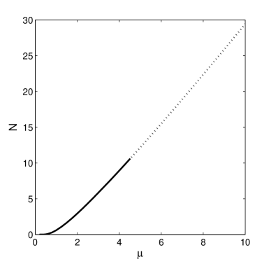
Figure 6: (a) A typical example of the first excited 1D symmetric state, for $x_{0}=1$, $\mu=5$ and $\alpha=0.5$. (b) The respective solution branch $N(\mu)$, for $x_{0}=1$ and $\alpha=0.5$. It is stable at $\mu<4.523$, i.e., $N<10.6059$.

Similar to the asymmetric mode, the stability of the first excited symmetric state strongly depends on $x_{0}$ and $\alpha$, see Fig. 7, the instability being always accounted for by complex eigenvalues. An example of the evolution of an unstable solution of this type is shown in Fig. 7. Like the unstable asymmetric and antisymmetric states presented above, it converges to a stable symmetric solution.

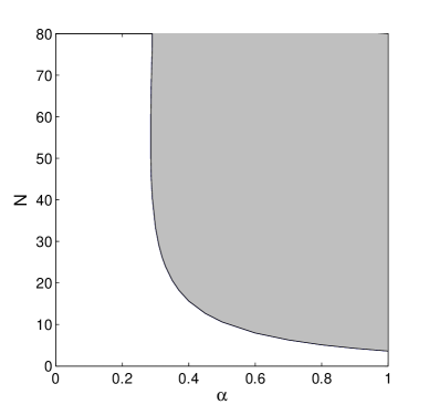
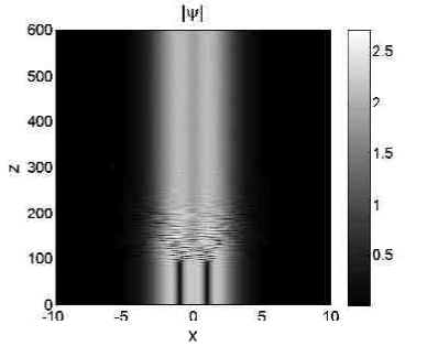
Figure 7: (Color online) (a) The stability diagram for the first excited 1D symmetric state (an example of which is shown in Fig. 6), in the $\left(\alpha,N\right)$ plane, for $x_{0}=1$. As above, the white and gray regions represent stable and unstable solutions, respectively. (b) The evolution of an unstable first excited symmetric state, for $x_{0}=1$, $\alpha=0.5$ and $\mu=7$.

Also found was a second excited symmetric state, an example of which is shown in Fig. 8 for $x_{0}=1$, $\mu=5$ and $\alpha=0.5$. This mode is composed of two $k=2$ single-well solutions, where, as mentioned above, $k$ is the number of nodes (zeroes) of the 1D mode trapped in the single nonlinear pseudopotential well Barcelona2 . Results for this solution family and its stability, for $x_{0}=1$ and $\alpha=0.5$, are presented in Fig. 8, and the dependence of the solution’s stability on $\alpha$ is shown in Fig. 9

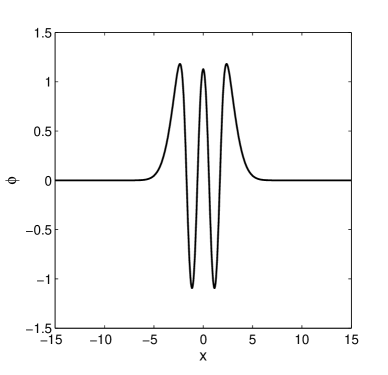
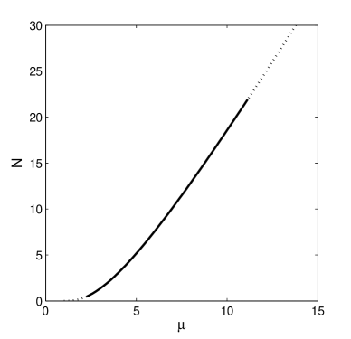
Figure 8: (a) A typical example of the second excited 1D symmetric state, for $x_{0}=1$, $\mu=5$ and $\alpha=0.5$. (b) The $N(\mu)$ curve for these solutions. The stability segment is $2.26<\mu<11.13$, i.e., $0.48<N<21.93$.

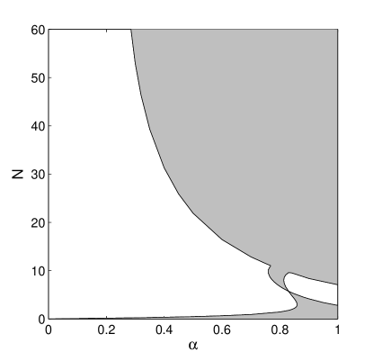
Figure 9: The stability diagram for the second excited 1D symmetric state, in the $\left(\alpha,N\right)$ plane, for $x_{0}=1$. The solutions are stable in white regions.

Similar to the unstable antisymmetric and asymmetric states considered above, the instability of the second excited symmetric states is accounted for by complex eigenvalues. The development of the instability transforms them into stable fundamental symmetric states, via a stage of oscillatory behavior. The latter stage is very long for low values of $\mu$ (or $N$), shrinking at larger $\mu$ (not shown here in detail).

Alongside the higher-order symmetric states introduced above, higher-order asymmetric solutions were found too. An example is a family of composite asymmetric states of the $[k=0,k=2]$ type, which are introduced in Fig. 10, for $x_{0}=1$, $\mu=5$ and $\alpha=0.5$. This mode is a combination of two single-well-based constituents: a fundamental solution on one side ($k=0$), and a solution with two nodes ($k=2$) on the other. Figure 10 exhibits a typical $N(\mu)$ branch for this type of composite modes. It is seen that the branch consists of two, almost coinciding, curves that merge at a certain point (in the present case, at $\mu=8.17$, $N=24.07$), with only the lower curve having a stability segment.

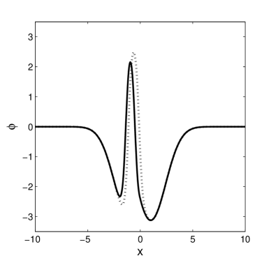
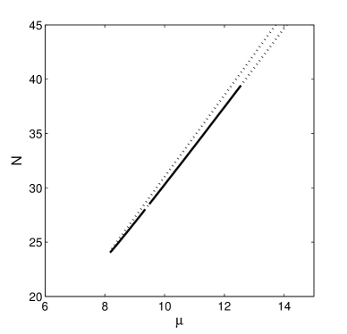
Figure 10: (a) The solid and dotted profiles show, severally, examples of stable and unstable composite 1D asymmetric solutions of the [$k=0,k=2$] type, for $x_{0}=1$, $\mu=10$ and $\alpha=0.5$. (b) $N(\mu)$ curves of the composite asymmetric states of these types, also for $x_{0}=1$ and $\alpha=0.5$. Two stable(solid) segments were found on the lower branch: at $8.17<\mu<9.34$, i.e., $24.05<N<27.98$, and at $9.49<\mu<12.54$, i.e., $28.51<N<39.38$.

The stability map for this type of the asymmetric composite modes in the plane of $\left(\alpha,N\right)$ is shown in Fig. 11. It exhibits not a single stability region, but a more complex map, with internal instability strips. The dark region at low values of $N$ (or $\mu$) refers to the region where the solutions do not exist, above the merger point of the two branches. Similar to what was shown before for symmetric unstable modes [see Fig. (7)], the evolution of unstable asymmetric composite modes originally exhibits an oscillatory behavior, leading to transformation into the stable fundamental symmetric mode (not shown here in detail).

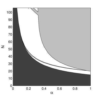
Figure 11: The stability diagram of the composite 1D modes of the $[k=0,k=0]$ type in the $\left(\alpha,N\right)$ plane, for $x_{0}=1$. Solutions do not exist in the dark region at the bottom of the plot. As above, the solutions are unstable in gray areas.

The relative stability of the different coexisting modes with equal norms is determined by the comparison of their Hamiltonians, given by the 1D version of Eq. (2). The respective $H(N)$ curves for all the above-mentioned 1D solutions are displayed in Fig. 12, for $x_{0}=1$, $\alpha=0.5$. As expected, the ground state, with the lowest value of the Hamiltonian, corresponds to the basic symmetric solution, while the first and second excited symmetric states have, respectively, higher values of $H$.

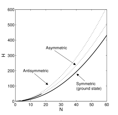
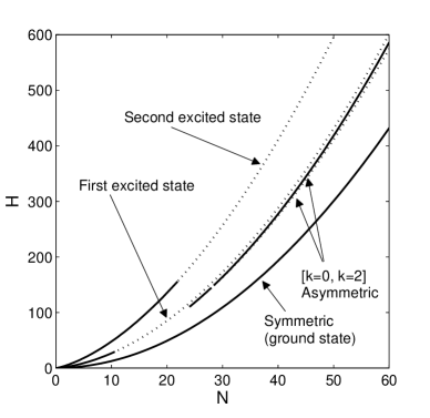
Figure 12: The Hamiltonian-versus-norm curves for families of 1D states, at $x_{0}=1$ and $\alpha=0.5$. Continuous and dotted lines refer to stable and unstable solutions, respectively. Panel (a) exhibits the curves for the basic symmetric, antisymmetric and asymmetric states. The composite asymmetric state of the $[k=0,k=2]$ type, as well as the first and second excited symmetric modes, are presented in panel (b) (the curve for the basic symmetric solutions, which represent the ground state, is included in both panels, for the sake of comparison).

II.3 The general 1D model: asymmetric modes

In addition to the detailed investigation reported above for the simplest version of the DW profile, based on Eq. (9), a partial analysis has been performed for the more general profile corresponding to Eq. (8). Specifically, we have examined the influence of parameters $\sigma_{0}$ and $\sigma_{2}$ on the stability of the asymmetric state. Figure 13 displays the respective stability diagram in the $\left(\alpha,N\right)$ plane, with $\sigma_{0}=1$, $\sigma_{2}=2$, $x_{0}=1$, and $\beta=0$. Similar results were also obtained for $\beta=1$ (not shown here). As seen in Fig. 13, asymmetric solutions were found for all values of $\alpha$, provided that the soliton’s norm is high enough (an expected outcome, as the effective DW potential depends on $N$). The stability region expands with the increase of $\alpha$, opposite to what is reported above for the simplified profile (9), cf. Fig. 3. When the constant term is absent, $\sigma_{0}=0$, the stability map features alternating stability and instability strips, as seen in Fig. 13(b). For the same parameters, but with $\sigma_{0}=1$ [Fig. 13(a)], the striped pattern, barely observed at small values of $\alpha$, is much less salient.

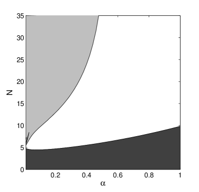
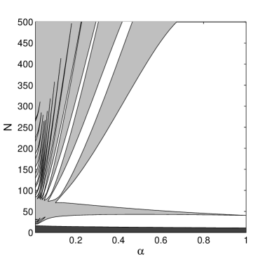
Figure 13: Stability diagrams for 1D asymmetric modes, obtained with the generalized nonlinearity-modulation profile (8), for $\sigma_{2}=2$, $x_{0}=1$, $\beta=1$, and (a) $\sigma_{0}=1$ or (b) $\sigma_{0}=0$. White and gray regions represent, as before, stable and unstable solutions, respectively. The asymmetric solutions do not exist in the dark region at the bottom of the plots, below the bifurcation of the antisymmetric mode.

III A rocking one-dimensional potential well

It is natural to extend the consideration of modes trapped in the single (pseudo)potential well to the case when the well is subject to rocking motion, which corresponds to

$$\sigma(z)=\exp\left[\alpha(x-A_{0}\cos(W_{0}z)^{2})\right]$$ (15)

in the 1D version of Eq. (1), where the $A_{0}$ and $W_{0}$ are the rocking amplitude and frequency. In the optical realization, this corresponds to to the planar waveguide with an undular guiding channel [in the plane of $\left(z,x\right)$], written by the local modulation of the defocusing nonlinearity rocking-optical . In the case of BEC, the rocking implies oscillatory motion of the nonlinearity-modulation profile, which can be readily implemented if the modulation is induced by the optically-controlled Feshbach resonance FR-Tom , as the controlling laser beam may be made moving painting .

Here, we focus on the fundamental and first-order (dipole) modes, both well-known to be stable in the static model Barcelona . In all the examples shown below, we fix $\alpha=0.5$, while the parameters of the rocking well were taken in ranges $0<A_{0}<4$ and $2\pi/40<W_{0}<2\pi$.

Starting with the fundamental modes, two evolution scenarios can be identified, depending on the initial value of the norm, $N$ (or $\mu$), and parameters $A_{0}$ and $W_{0}$. Namely, for the rocking period, $Z_{0}=2\pi/W_{0}$, exceeding a certain threshold value, the mode adiabatically follows the slowly rocking nonlinear well, maintaining its original shape. An example is shown in Fig. 14.

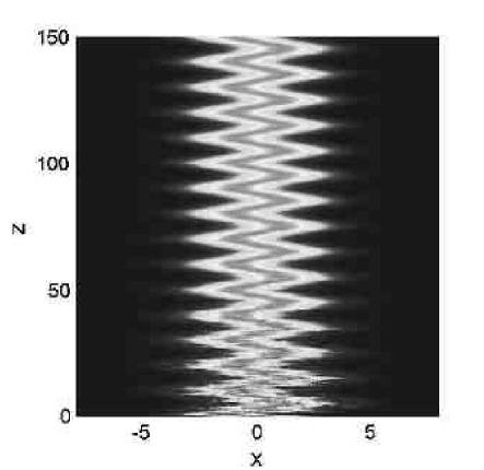
Figure 14: (Color online) An example of the stable evolution of a 1D fundamental mode, with $\mu=5$ ($N=12.22$), which adiabatically follows the single-well rocking with a large period, $Z_{0}=10$, and amplitude $A_{0}=1$.

On the other hand, for period $Z_{0}$ below this threshold, the shape of the initial fundamental soliton is not kept. In this case, the evolution of the solution is not smooth, and may exhibit different oscillatory patterns. Examples are shown in Fig. 15 for $\mu=5$, $A_{0}=1$ and $Z_{0}=4$ and $5$. Further, the dependence of the threshold value of the rocking period on the rocking amplitude, $A_{0}$, is shown in Fig. 16, for two fixed values of the norm.

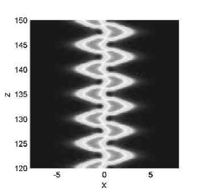
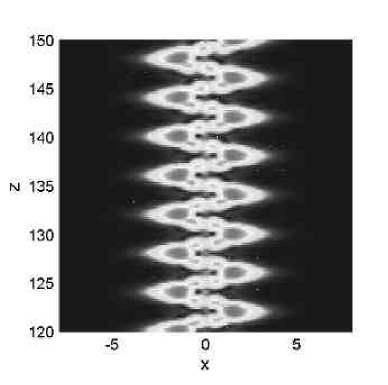
Figure 15: (Color online) Typical examples of the non-adiabatic evolution of the 1D fundamental mode, in the case of relatively fast rocking motion of the underlying nonlinear well. For $\mu=5$, $A_{0}=1$ and $Z_{0}=5$ (a), the wave pattern keeps a single-peak shape. With the rocking period further (slightly) decreasing to $Z_{0}=4$, the pattern breaks into fragments.

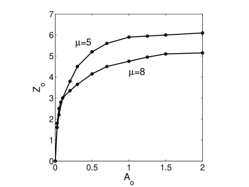
Figure 16: The threshold value of the rocking period, below which the evolution of the trapped 1D fundamental mode is non-adiabatic, see Fig. 15. Two curves pertain to fixed $N=12.22$ (the respective propagation constant in the absence of the rocking is $\mu_{0}=5$) and $N=19.74$ ($\mu_{0}=8$).

The evolution of the trapped dipole mode also turns out to be different above and below the threshold value of the rocking period, which is found to be virtually indistinguishable from the one shown in Fig. 16 for the fundamental solution. Below the threshold, the dipoles quickly transform into single-peak or fragmented patterns, which are quite similar to those observed in the case of the fundamental mode, see typical examples in Fig. 17 for $\mu=5$, $A_{0}=1$ and $Z_{0}=4$ or $5$.

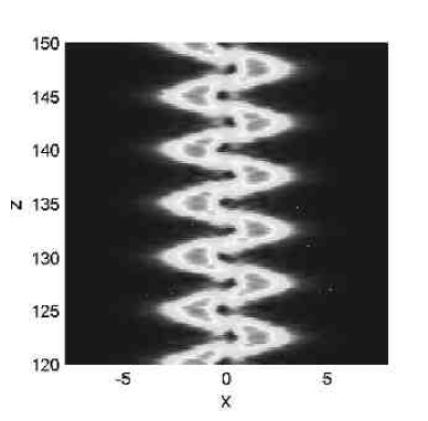
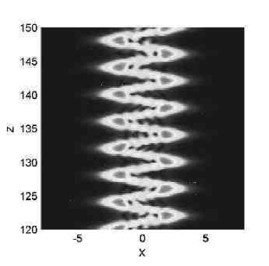
Figure 17: (Color online) The evolution of the 1D dipole mode trapped in the single rocking nonlinear well below the threshold, when the initial profile is destroyed. Similar to the situation with the fundamental mode (see Fig. 15), the dipole transforms into an oscillating single-peak pattern, at $\mu=5$, $A_{0}=1$ and $Z_{0}=5$ (a). At a still smaller rocking period, $Z_{0}=4$, the solution breaks into fragments (b).

On the other hand, when the rocking period is taken above the threshold, the mode periodically switches between the initial dipole shape and the fundamental soliton. This scenario, which may be considered as Rabi oscillations between the two soliton species (dipole and fundamental ones) in the rocking (pseudo)potential well Rabi , is demonstrated in Fig. 18 for $N=7.92$ (the respective propagation constant, corresponding to the dipole mode in the absence of the rocking, is $\mu=5$).

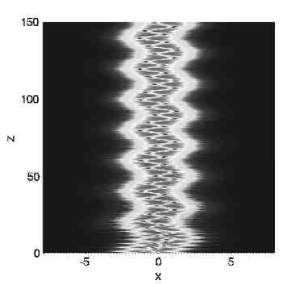
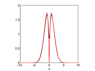
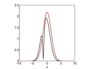
Figure 18: (Color online) (a) A typical example of the evolution of the1D dipole solution trapped in the slowly rocking nonlinear well (above the threshold value of the period), which results in Rabi oscillations between the dipole (b) and single-peak fundamental (c) modes. The parameters are $N=7.92$, $A_{0}=0.5$ and $Z_{0}=20$. Panels (b) and (c) compare the shapes of the periodically appearing fundamental and dipole modes (shown by black curves), and their stationary counterparts with the same norm (plotted by red curves).

Unlike the destructive oscillations below the threshold (see Fig. 17), the frequency of the Rabi oscillations above the threshold is different from the rocking frequency, $W_{0}$. Figure 19 shows the period of the intrinsic Rabi oscillations of the trapped mode, $Z_{\mathrm{i}}$, as a function of $N$. Detailed numerical analysis demonstrates that $Z_{\mathrm{i}}$ is insensitive to the rocking parameters, $Z_{0}$ and $A_{0}$. This feature is demonstrated in Fig. 20, where the frequency of the Rabi oscillations remains constant, while the rocking frequency varies. Thus, the Rabi oscillations between the fundamental and dipole states are actually a dynamical feature of the system based on the stationary profile of the nonlinearity modulation, while the rocking motion is a drive which helps to excite the oscillations.

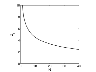
Figure 19: (Color online) The period of the Rabi (intrinsic) oscillations of the trapped 1D mode between the dipole and fundamental shapes, $Z_{\mathrm{i}}$, as a function of $N$.

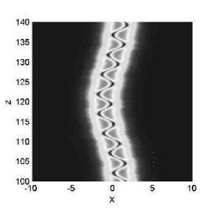
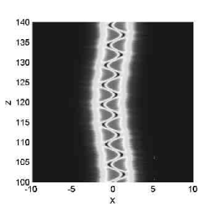
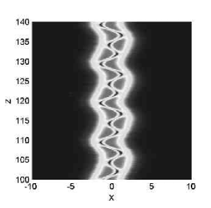
Figure 20: (Color online) Examples of the Rabi oscillations of the 1D trapped mode: (a) $A_{0}=1$, $Z_{0}=40$; (b) $A_{0}=0.5$, $Z_{0}=40$; (c) $A_{0}=0.5$, $Z_{0}=10$. In all the cases, $N=7.92$.

Actually, the Rabi oscillations are not completely robust. Gradually, the oscillations fade away, and the trapped mode slowly relaxes into the fundamental solution. The evolution period in the course of which the Rabi oscillations remain conspicuous reduces with the increase of the underlying rocking amplitude, $A_{0}$, and frequency, $W_{0}$.

IV The two-dimensional setting: the single-well nonlinear potential

The existence and stability of the axially-symmetric states, both fundamental (zero-vorticity) ones and vortices with a nonzero topological charge, in the 2D model with the isotropic single-well modulation profile, based on Eq. (7) with $\mathbf{r}_{0}=0$, including the simplified version (6), were reported in Ref. Barcelona2 . In this section we introduce and briefly consider additional higher-order modes, both nontopological and topological ones, which demonstrate the SSB effect in the form of spontaneous breaking of the axial symmetry. This setting, which is fundamental by itself, deserves a detailed study, results of which will be reported elsewhere Radik .

Examples of first-, second- and third-order states, which may be interpreted, respectively, as dipoles, “string tripoles” and “string quadrupoles”, are displayed in Fig. 21, for $\mu=5$ and $\alpha=0.5,$ the respective $N(\mu)$ curves being shown, for $\alpha=0.5$, in panel (d) of the figure. Direct simulations have demonstrated that families of the second- and third-order solutions are entirely unstable, and it is reasonable to conclude that their counterparts of still higher orders are unstable too. The instability-induced evolution transform the unstable modes into the ground state, as shown in Fig. 22 for an unstable dipole. On the other hand, as shown in Fig. 23, dipoles have a narrow stability interval at small values of $\mu$ (or $N$) (to the left of the red dot in the figure), which will be reported in detail in another work Radik .

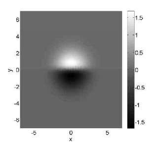
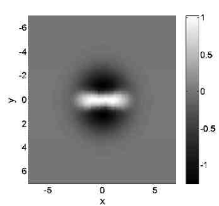
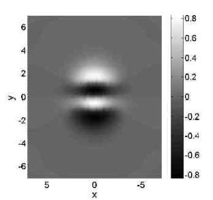
Figure 21: (Color online) Examples of unstable anisotropic higher-order 2D solutions, produced by stationary equation (4), with the single-well nonlinearity-modulation profile (6). Panels (a), (b) and (c) display examples of dipoles, “string tripoles”, and “string quadrupoles”, respectively, for $\mu=5$ and $\alpha=0.5.$

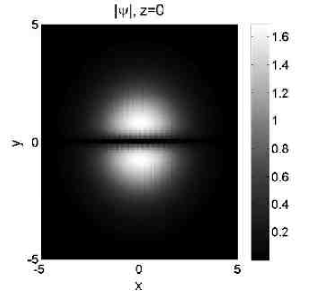
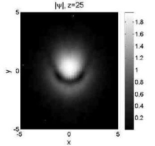
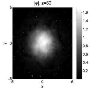
Figure 22: (Color online) The evolution of an unstable 2D dipole mode (the “first order” state from Fig. 21), at $\mu=5$ and $\alpha=0.5$.

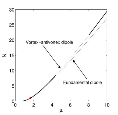
Figure 23: (Color online) The red dot (at $\mu=1.64,N=0.98$) marks the bifurcation of the family of VADs (vortex-antivortex dipoles) from the fundamental-dipole-mode branch in the single nonlinear 2D potential well, for $\alpha=0.5$. As before, solid and dashed curves refer to stable and unstable states, respectively. The fundamental-dipole-mode branch is destabilized at the bifurcation point.

More interesting 2D topological states trapped in the single nonlinear potential well are vortex-antivortex dipoles (VADs), shaped as fundamental solutions with an embedded pair of vortical holes carrying opposite topological charges, $\pm 1$, so that the total charge is zero, see an example in Fig. 24 for $\mu=5$ and $\alpha=0.5$. Systematic results for this family will be presented in Ref. Radik . In particular, it bifurcates, as a stable branch, from the family of the above-mentioned ordinary (fundamental) dipoles, as shown in Fig. 23. With the increase of $\mu$ and $N$, the VAD gets destabilized by oscillatory perturbations, and then restabilizes.

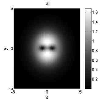
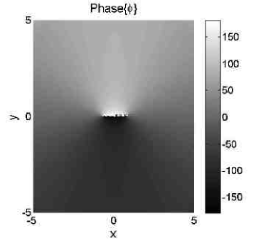
Figure 24: (Color online) An example of the amplitude (a) and phase (b) structure of a stable vortex-antivortex dipole trapped in the single 2D nonlinear well, for $\mu=5$ and $\alpha=0.5$. Here and in similar patterns displayed below, values of the phase are given in degrees (not in radians).

The branch of $m=2$ vortices gives rise, via a bifurcation, to another anisotropic topologically charged mode trapped in the single nonlinear potential well, namely, vortex triangles (VTs), see an example in Fig. 25 for $\mu=7$, $\alpha=0.5$. As shown in Fig. 26, this family indeed bifurcates, at

$$\mu=5.73,N=19.2$$ (16)

(if $\alpha=0.5$ is fixed), from the ordinary stable vortex branch with $m=2$, which was constructed, in the framework of the present model, in Ref. Barcelona2 . Figure 25(b) confirms that, following its parent vortex mode, the VT carries topological charge $m=2$. The fact that the triangular vortical state emerges from the double-charged vortex is a counter-intuitive manifestation of the SSB in the present setting, which, however, does not contradict general principles. Note that the present VT modes are different from rotating triangles built of well-separated unitary vortices, which were observed, as a dynamical regime initiated by splitting of unstable vortices with topological charge $m=3$ (rather than $m=2$), in the same model Barcelona2 .

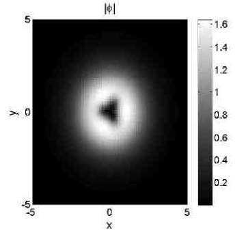
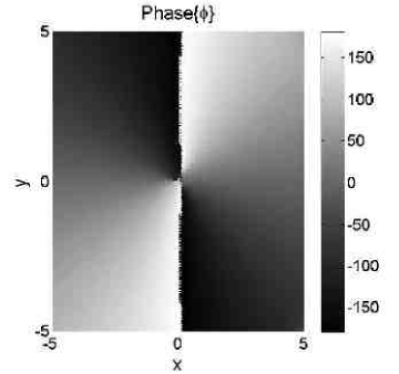
Figure 25: (Color online) The amplitude (a) and phase (b) structure of a vortex triangle supported by the single 2D nonlinear potential well, at $\alpha=0.5$, $\mu=7$ ($N=25.86$). This mode is weakly unstable, see Fig. 26 below.

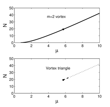
Figure 26: The $N(\mu)$ curves, demonstrating, for $\alpha=0.5$, the bifurcation of the the VT (vortex-triangle) branch (the bottom panel), from the family of ordinary stable vortices with topological charge $m=2$ (the upper panel; the curves are displayed in the different panels, as they would otherwise completely overlap). The circles mark, in both panels, the bifurcation point, at $\mu=5.73,N=19.2$. As before, solid and dotted lines refer to stable and unstable solutions, respectively. The short dashed bold segment refers to spinning VTs.

The stability analysis of the VTs demonstrates that, strictly speaking, the entire family is unstable. Further, direct simulations of the perturbed evolution demonstrate that, from bifurcation point (16), at which this branch appears, and up to $\mu=6.55$ ($N=23.43$), the VT exhibits rotation, as a robust object, at an angular velocity whose value depends on the initial perturbation. The rotation interval is designated by the (short) dashed bold segment in the bottom panel of Fig. 26). An example for such a spinning VT is shown in Fig. 27 for $\mu=6$.

At $\mu>6.55$, the VTs develop real instability, evolving into the above-mentioned stable VADs, see an example in Fig. 28, or into the ground state, as observed above for other species of unstable modes.

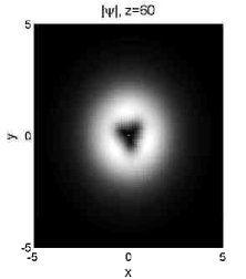
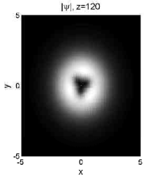
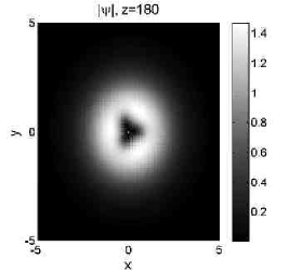
Figure 27: (Color online) The evolution of a robust vortex triangle, trapped in the single nonlinear potential well, at $\alpha=0.5$ and $\mu=6$ ($N=20.58$), with an initial perturbation that slightly increases its norm. The result is a triangle steadily rotating in the clockwise direction.

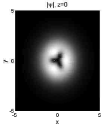
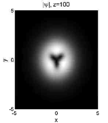
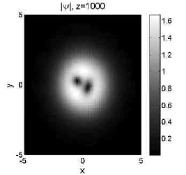
Figure 28: (Color online) The evolution of an unstable vortex triangle at $\alpha=0.5$ and $\mu=7$ ($N=25.86$).

The systematic numerical analysis has revealed other species of anisotropic modes trapped in the single isotropic nonlinear potential well. In particular, bound states of multiple (more than three) vortices were observed. One such species, a “vortex hexagon” with zero total topological charge, which is shown in Fig. 29, bifurcates from the unstable branch of tripoles from Fig. 21(b). This state, as well all other bound states of many vortices, are completely unstable.

Another type of solutions, in the form of isotropic higher-order (alias, excited) radial states of vortices, were found too, for the first time in the model of the present type. An example of an excited radial state of the vortex solution, with $m=1$ and one radial node (zero), is shown in Fig. 30. These solutions are unstable too, relaxing into the stable basic vortices (with the node-free radial structure).

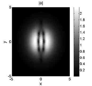
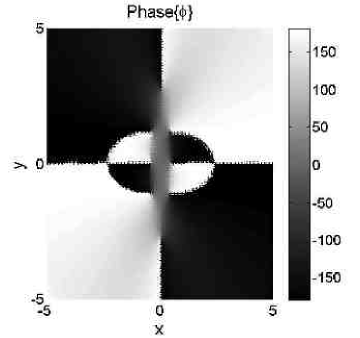
Figure 29: (Color online) An example of the amplitude (a) and phase (b) structure of an unstable vortex hexagon trapped in a single nonlinear potential well, for $\mu=10$, $\alpha=0.5$.

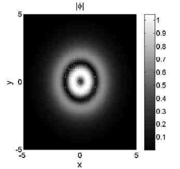
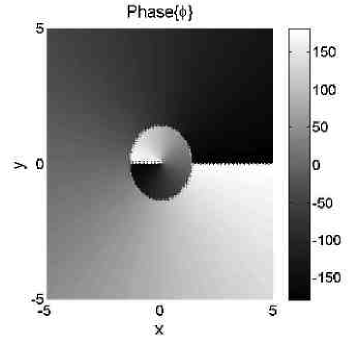
Figure 30: (Color online) An example of the amplitude (a) and phase (b) structure of an unstable excited radial vortex state, with $m=1$, $\mu=5$ and $\alpha=0.5$.

V The two-dimensional setting: the double-well (DW) nonlinear potential

V.1 Zero-vorticity states

The most essential object of the 2D analysis is the model with the DW nonlinearity profile, represented by Eq. (9), focusing on SSB scenarios in this setting (cf. a 2D DW profile based on the spatial modulation of the self-focusing nonlinearity, which was introduced in Ref. 2D-Thawatchai ). The respective fundamental symmetric state is illustrated by Fig. 31, for $\mu=5,\alpha=0.5$ and $x_{0}=1$. Direct simulations have shown that this state is stable for all values of $x_{0}$, $\mu$ and $\alpha$, with the respective $N(\mu)$ curve for $\alpha=0.5$ and $x_{0}=1$ displayed in Fig. 31).

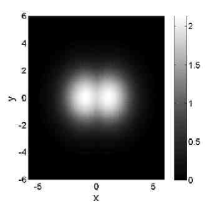
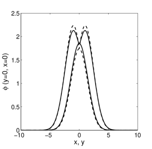
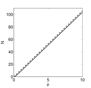
Figure 31: (Color online) (a) A typical example of the 2D stable symmetric fundamental state in the model with the double-well nonlinearity profile [see Eq. (9)] for $\mu=5$ $\alpha=0.5$ and $x_{0}=1$. (b) The cross-section profiles of the same solution, drawn through $x=0$ and $y=0$. The solid and dashed lines display, respectively, the numerically found solution and its counterpart produced by the TFA (Thomas-Fermi approximation) based on Eq. (17). (c) The respective $N(\mu)$ curve of stable symmetric solutions for $\alpha=0.5$ and $x_{0}=1$, with the dashed line representing the respective TFA given by Eq. (18).

This 2D symmetric state can be easily found in the approximate form in the framework of the TFA, cf. its 1D version (13):

$$\phi_{\mathrm{TFA}}(x,y)=\sqrt{\mu}\exp\left\{-\left(\alpha/2\right)\left[\left(|x|-x_{0}\right)^{2}+y^{2}\right]\right\},$$ (17)

the corresponding approximation for the norm being [cf. the 1D result (14)]:

$$N_{\mathrm{TFA}}(\mu)=\left(\pi/\alpha\right)\mu\left[1+\mathrm{erf}\left(\sqrt{\alpha}x_{0}\right)\right].$$ (18)

The latter result readily explains the nearly linear numerically found dependence $N(\mu)$ displayed in Fig. 31(b).

Antisymmetric zero-vorticity states, as well as asymmetric ones bifurcating from them, have been found too, but they turn out to be completely unstable (not shown here in detail), unlike their 1D counterparts, cf. Figs. 2 and 3. In direct simulations, unstable states of these type spontaneously rearrange into stable symmetric modes.

V.2 Semi-vortices trapped in the double-well potential

Stable semi-vortex 2D states can be composed of fundamental and vortex modes supported, severally, by the two nonlinear wells. A representative example, built of the fundamental solution and the vortex with topological charge $m=1$, is displayed in Fig. 32(a,b), for $x_{0}=2.5$, $\mu=5$ and $\alpha=0.5$. The respective stability diagrams, produced by varying $\mu$ at fixed $x_{0}$, and varying $x_{0}$ at fixed $\mu$, are presented in Figs. 32(c,d). It is seen that the composite state readily gets stabilized with the increase of $x_{0}$: at $\mu=5$, the solution is stable for $x_{0}>2.18$. For $x_{0}=2$, the solution is unstable for all values of $\mu$ and $N$ (not shown here in detail), while, at $x_{0}=2.5$, it is stable for $\mu>1.12$, $N>7.63$. When the semi-vortex solutions are unstable, they evolve into stable symmetric fundamental states.

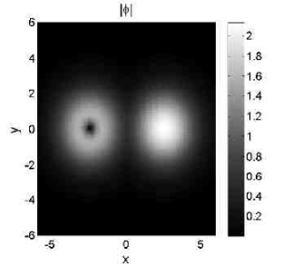
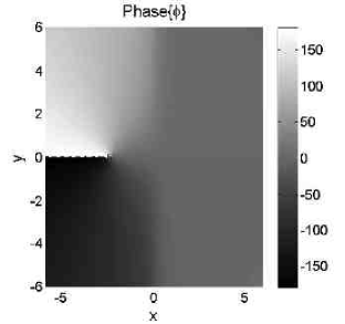
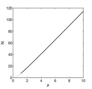
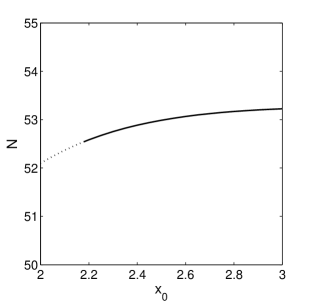
Figure 32: (Color online) (a,b) Amplitude and phase profiles of the semi-vortex composite state, built of a vortex with topological charge $m=1$ trapped in the left well, and a fundamental soliton trapped in the right well, for $x_{0}=2.5$, $\mu=5$ and $\alpha=0.5$. The respective $N(\mu)$ and $N\left(x_{0}\right)$ curves are displayed in panels (c) and (d), fixing $\alpha=0.5$ and $x_{0}=0.5$ or $\mu=5$, respectively.

For the semi-vortical complex built of the fundamental soliton and vortex with topological charge $m=2$, similar results were obtained, with an essential addition: the bifurcation of the VT occurs from its vortex component. Examples of composite modes of both types, including either the vortex component with $m=2$ or the VT generated by it, are displayed in panels (a)-(c) of Fig. 33 for $\mu=7$, the phase pattern being common to both. The stability of these complexes is presented in panels (d,e) of Fig. 33.

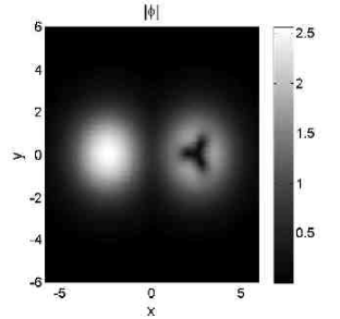
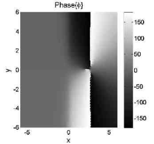
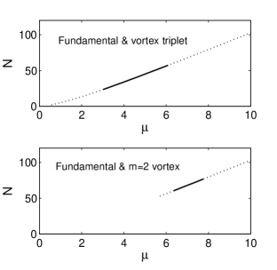
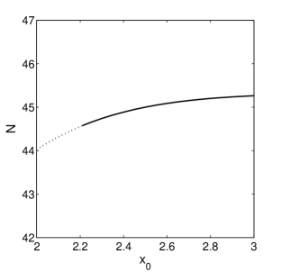
Figure 33: (Color online) (a)-(c) Amplitude profiles and a common phase pattern of 2D composite states built of a single-well fundamental mode in the left well, and a vortex with topological charge $m=2$, or a vortex triangle, bifurcating from it, in the right well, for $x_{0}=2.5$, $\mu=7$ and $\alpha=0.5$. (d) $N(\mu)$ curves for both species, at $\alpha=0.5$, $x_{0}=2.5$ (because of overlapping, the branches are shown separately). (e) The $N\left(x_{0}\right)$ plane, for $\mu=5$, below the bifurcation, where only the soliton-vortex complex exists.

In direct simulations, those semi-vortices with $m=2$ which are unstable turn into a stable complex built of a single-well fundamental state in one well and a VAD supported by the other. Following this observation, two different combinations of the fundamental soliton and VAD, supported by the individual wells, were investigated in detail: horizontal and vertical ones, with the line connecting centers of the two vortices (which built the VAD) oriented, respectively, parallel or perpendicular to the axis of the two-well configuration, see Figs. 34(a,b) and (c,d), respectively. The former species is partially stable: for instance, at $\mu=5$, it is stable for $x_{0}>1.70$, see Fig. 34. When fixing $x_{0}=2$, the stability region is $\mu>2.96$, $N>26.38$ (Fig. 34), while for $x_{0}=1.5$ the solution is entirely unstable. Complexes of the latter (perpendicular) type are always unstable, which can be understood, as only a horizontally aligned dipole may realize an energy minimum in the present setting. In both cases, unstable complexes converge to the ground-state symmetric modes.

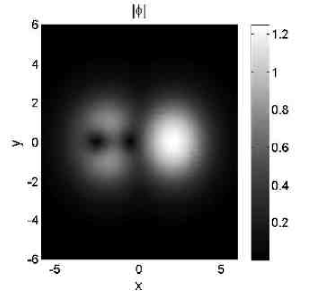
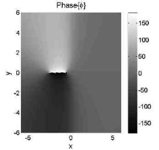
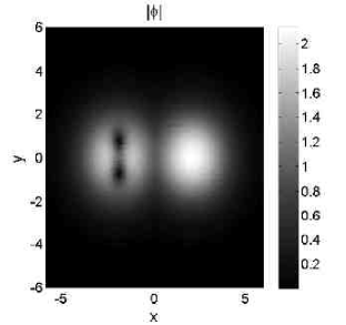
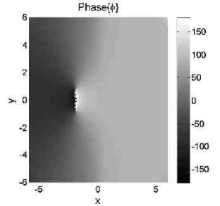
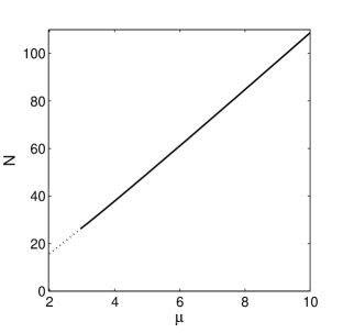
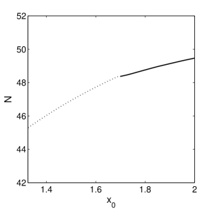
Figure 34: (Color online) Examples of semi-vortex complexes built of the single-well fundamental soliton in the right well, and a horizontal (a,b) or vertical (c,d) vortex-antivortex dipole in the left one, for $x_{0}=2$, $\mu=5$ and $\alpha=0.5$. Complexes of the vertical type are completely unstable. (e) The $N(\mu)$ curve for complexes of the horizontal type with $\alpha=0.5$ and $x_{0}=2$. (f) The corresponding $N\left(x_{0}\right)$ curve, for $\mu=5$.

V.3 Dual-vortex configurations supported by the double-well potential

Dual-vortex complexes, composed of vortices with $|m|=1$ trapped in the two wells, were constructed too. Figures 35(a,b) and (c,d) show examples of such complexes, built of individual vortices with topological charges $\left(m=+1,m=-1\right)$ or $\left(m=+1,m=+1\right)$, so that the respective total charges are $0$ or $2$. In both cases, the results are similar: the solutions are unstable at $x_{0}=2$, and stable at $x_{0}=2.5$. Fixing $\mu=5$, the $\left(+1,-1\right)$ complex is stable for $x_{0}>2.31$, $N>46.38$ (Fig. 35), while its counterpart of the $\left(+1,+1\right)$ type is stable at $\ x_{0}>2.26$, $N>46.21$ (Fig. 35). In this case too, unstable solutions transform themselves into symmetric ground-state modes.

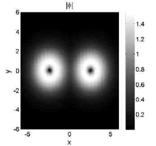
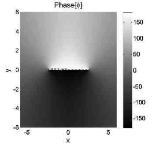
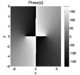
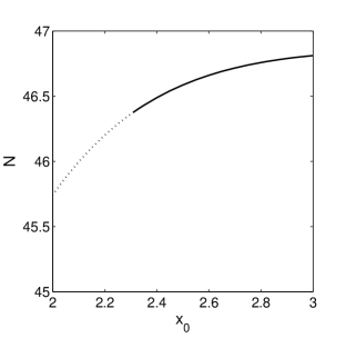
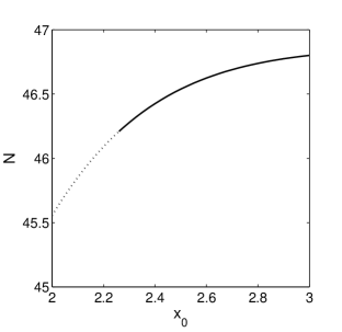
Figure 35: (Color online) Examples of dual-vortex complexes with topological-charge sets $\left(+1,-1\right)$ (a,b) and $\left(+1,+1\right)$ (c,d), for $x_{0}=2.5$, $\mu=5$ and $\alpha=0.5$. The $N(x_{0})$ curves, with $\mu=5$, for the complexes of these two types are displayed in panels (e) and (f), respectively.

Dual-vortex complexes built of vortices with $|m|=2$ were also addressed. In both cases of topological-charge sets $\left(+2,-2\right)$ and $\left(+2,+2\right)$, the transition (bifurcation) from the individual double vortices to the VTs occurs, thus giving rise to additional dual-VT complexes. An example of the complex for the charge set $\left(+2,-2\right)$ is displayed in Figs. 36(a,b), with the respective bifurcation diagram shown in Fig. 36. In this case, the dual-vortex complexes are stable at $5.71<\mu<7.96$, i.e., $37.92<N<61.73$. Further, an example of the related dual-VT complex, with the same charge set, $\left(+2,-2\right)$, and the same parameters is presented in Fig. 36(c,d). The dual-VT complexes of this type are stable at $3.05<\mu<6.07$, i.e., $12.69<N<41.52$. For $\mu=5$ and varying $x_{0}$, the dual-vortex complexes with topological charges $\left(+2,-2\right)$ are stable at $x_{0}>2.40$ for fixed $\mu=0.5$, as shown in Fig. 36 (in this case, VTs do not exist, as they are generated by the bifurcation at larger values of $\mu$).

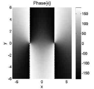
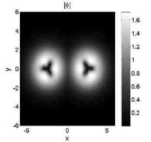
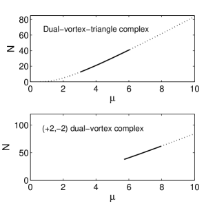
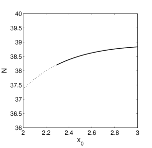
Figure 36: (Color online) Dual-vortex complexes with topological charges $\left(+2,-2\right)$, built of two single-well vortices (a,b), or vortex triangles (c,d), for $x_{0}=2.5$, $\mu=7$ and $\alpha=0.5$. (e) The respective $N(\mu)$ curves, for $x_{0}=2.5$ and $\alpha=0.5$. (f) The $N(x_{0})$ curve, for the dual-vortex complexes at fixed $\mu=5$.

Similar results for the complexes pertaining to the topological-charge set $\left(+2,+2\right)$ are presented in Fig. 37. Here, for $x_{0}=2.5$, the dual-vortex complexes, and ones built of the VTs, are stable at $6.74<\mu<7.71$, i.e., $48.37<N<58.82$, and $4.47<\mu<5.54$, i.e., $25.30<N<35.87$, respectively. For $\mu=5$, the solutions are stable at $x_{0}>2.45$, as shown in Fig. 37.

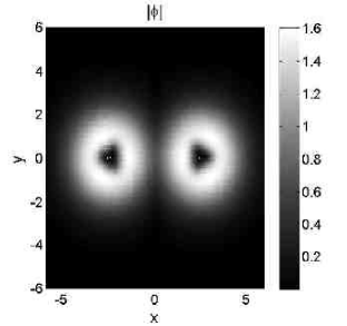
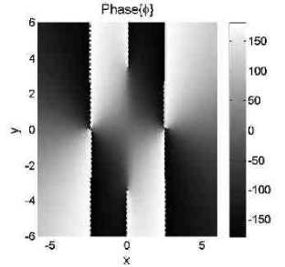
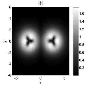
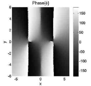
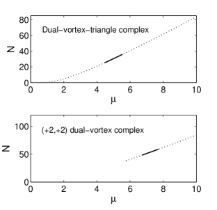
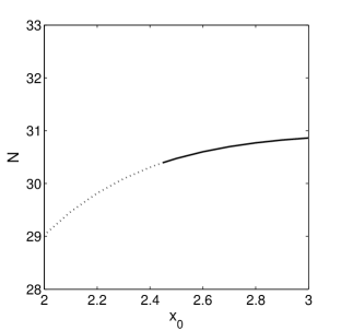
Figure 37: (Color online) The same as in Fig. 36, but for the vortex and vortex-triangle complexes with the topological-charge set $\left(+2,+2\right)$.

A conspicuous difference of the configuration with the charge set $(+2,+2)$ from the above one with charges $(+2,-2)$, observed in Fig. 37(a) [cf. Fig. 36(a)], is relatively strong deformation of cores of both left and right vortices. This is explained by attractive and destructive interference of overlapping fields of the vortices in the gap between their cores, in the cases of opposite and identical signs of the two vorticities, respectively. Indeed, in the latter case the destructive interference removes the field from the gap, making inner boundaries of the cores nearly flat, as seen in Fig. 37(a). A similar argument helps to understand the difference between the mutual orientations of the VTs, which is observed in Figs. 36(c) and 37(c): the interferometric removal of the field from the inter-core gap in the configuration case makes it possible to keep the empty corners inside the gap.

It is relevant to mention too that the stability regions are somewhat smaller for the complexes with the charge set $(+2,+2)$ than for their counterparts with charges $(+2,-2)$. Note that the difference between the dual-vortex complexes corresponding to charge sets $\left(+m,-m\right)$ and $\left(+m,+m\right)$ is much smaller in the case of $m=1$ than for $m=2$, cf. Fig. 35. This is explained by the fact that the size of the vortex core is essentially smaller for $m=1$.

All the complexes with $|m|=2$ are completely unstable at $x_{0}=2$. Direct simulations show that unstable solutions of these types transform themselves into the ground-state symmetric state, or into symmetric complexes of VADs (their description is following below). On the contrary to the VTs in the single-well case (see Fig. 27), the triangles forming stable dual-VT complexes in the DW potential do not exhibit rotation when perturbations are added to the initial configuration.

Dual-vortex composites, constructed of an $|m|=1$ vortex trapped in one well, and an $|m|=2$ vortex in the other, were also investigated. In this configuration, two families, with topological charges $\left(+1,+2\right)$ and $\left(-1,+2\right)$, were examined. Similar to the dual vortex complexes with $|m|=2$ mentioned above, bifurcations of structures, with the same charges, where VTs replace the vortex with $|m|=2$, are observed. An example of the vortex-vortex complex with the charge set $\left(+1,+2\right)$ is demonstrated in Fig. 38(a,b), for $\mu=7$ and $x_{0}=2.5$. For this charge set, the bifurcation diagram in the $\left(N,\mu\right)$ plane is displayed in Fig. 38 for $x_{0}=2.5$. In this case, the vortex-vortex complexes are stable at $6.58<\mu<7.84$, i.e., $56.02<N<70.36$. The corresponding vortex-VT complexes with charges $\left(+1,+2\right)$, demonstrated in Fig. 38(c,d) for $\mu=7$ and $x_{0}=2.5$, are stable at $3.01<\mu<5.91$, i.e., $17.85<N<48.50$. When fixing $\mu=5$ and varying $x_{0}$, the complexes with topological charges $\left(+1,+2\right)$ are stable at $x_{0}>2.29$.

Equivalent results were also observed for the other charge set, $\left(-1,+2\right)$, see Fig. 39). Examples of the vortex-vortex and vortex-VT structures, in this topological setting, are displayed in Figs. 38(a,b) and Figs. 38(c,d), respectively, for $\mu=7$ and $x_{0}=2.5$. For $x_{0}=2.5$, the vortex-vortex complexes are stable at $6.07<\mu<9.07$, i.e., $50.41<N<84.65$, and the vortex-VT ones are stable at $2.11<\mu<6.24$, i.e., $9.69<N<52.27$ (Fig. 39). As seen in Fig. 39, for fixed $\mu=5$, the stability holds at $x_{0}>2.36$.

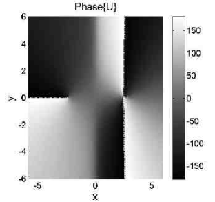
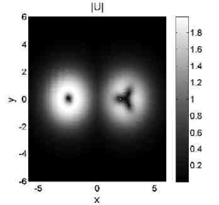
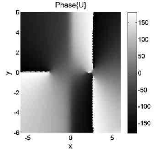
Figure 38: (Color online) Examples of dual-vortex mixtures, with the topological-charge set $\left(+1,+2\right)$, composed of $m=1$ and $m=2$ vortices trapped in the two wells (panels a and b), or an $m=1$ vortex and a VT (vortex triangle) (panels c and d), both for $x_{0}=2.5$, $\mu=7$. The $N(\mu)$ curves for both families, are presented in panel (e), for fixed $x_{0}=2.5$. Panel (f) shows the respective $N(x_{0})$ curve, for $\mu=5$.

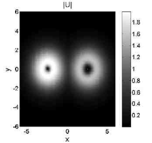
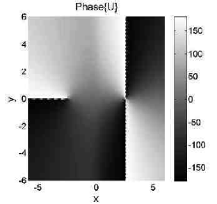
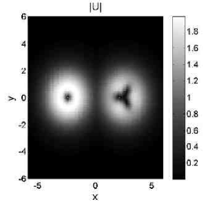
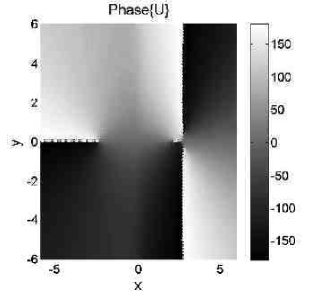
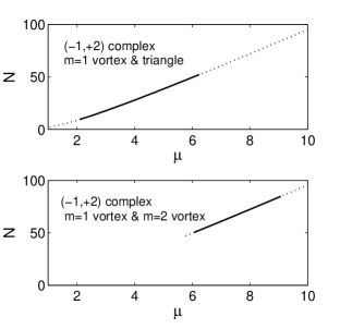
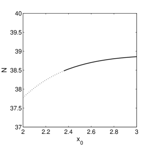
Figure 39: (Color online) The same as in Fig. 38, but for the vortex-vortex and vortex-VT complexes with the topological-charge set $\left(-1,+2\right)$.

Lastly, four combinations of VADs, of the horizontal and vertical types, as well as with identical or opposite orientations of the left and right dipoles, were constructed and analyzed too, see Fig. 40(a-h). A single species among them which was found to be partly stable corresponds to the horizontal structure shown in Fig. 40(c,d), in which the left and right components have opposite signs (recall that the semi-vortex complex with a VAD component may also be stable solely in the case when this component is horizontal, see Fig. 34; an explanation for the feasible stability of the horizontal structure in the present case is essentially the same, as only the horizontal orientation of the dipoles may realize an energy minimum). For this solution, the $N(\mu)$ curve, with fixed $x_{0}=3$ [Fig. 40], and the $N(x_{0})$ one, with fixed $\mu=5$ [Fig. 40], exhibit stability regions at $\mu>5.15$ and $x_{0}>3.05$, respectively. The unstable solutions evolve into the symmetric ground-state mode, or, in some cases, into stable combinations of VADs. In addition to these four complexes built of parallel VADs, another one, composed of a vertical VAD in one well and a horizontal VAD in the other, was also constructed. This state (which is not shown here), is entirely unstable

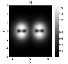
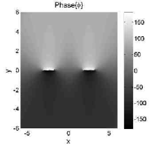
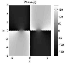
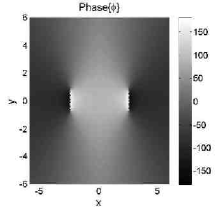
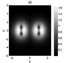
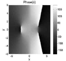
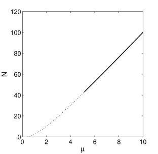
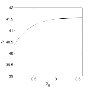
Figure 40: (Color online) (a)-(h) Four different combinations of two single-well VADS (vortex-antivortex dipoles), for $x_{0}=2.5$, $\mu=5$ and $\alpha=0.5$. (i) The $N(\mu)$ curve, for the single (partly) stable combination, shown in (c,d), for $x_{0}=3$ and $\alpha=0.5$. (j) The $N(x_{0})$ curve for the same family, at $\mu=5$.

To complete the study of dual-vortex complexes, it is relevant to mention that ones of both $\left(+m,-m\right)$ and $\left(+m,+m\right)$ types, composed of vortices proper (with $m=1$ and $2$) or VTs, as well as the VAD complexes with identical or opposite orientations, do not demonstrate spontaneous breaking of their symmetry or antisymmetry with respect to the underlying DW structure, in the entire parameter region explored in our analysis. Recall that, as mentioned above, antisymmetric complexes composed of 2D fundamental modes feature spontaneous breaking of the antisymmetry, but both the resulting asymmetric complexes and the antisymmetric parent ones are completely unstable.

VI Conclusion

The purpose of this work is to extend the analysis of the recently introduced class of models which admit self-trapping of stable solitons, vortices, and more complex topologically structured modes, with the help the defocusing cubic nonlinearity whose local strength grows fast enough from the center to periphery. In addition to the previously studied models with the single-well profile of the nonlinearity modulation, we have introduced the DW (double-well) settings in the 1D and 2D geometry, which may be realized in nonlinear optics and BEC. In both cases of the single- and double-well profiles, we have investigated various scenarios of the spontaneous formation of self-trapped modes, both nontopological and topological ones, whose symmetry may be lower than that of the underlying modulation pattern, due to the occurrence of the SSB (spontaneous symmetry breaking) in these systems. In particular, in the 2D single-well setting we have found unstable tripole and quadrupole modes and, on the other hand, partly stable ordinary (fundamental) dipoles, VADs (vortex-antivortex dipoles) and VTs (vortex triangles). The most essential results are reported for the DW settings, in 1D and 2D alike. Due to the repulsive sign of the nonlinearity, symmetric modes are always stable, realizing the system’s ground state. However, the antisymmetric (dipole) states are subject to the SSB (more accurately speaking, this is spontaneous breaking of the antisymmetry). The resulting asymmetric states are partly stable in 1D, but unstable in 2D. While most results have been obtained in a numerical form, the1D and 2D symmetric states were analyzed by means of the TFA (Thomas-Fermi approximation). Stability domains have been identified for diverse 2D semi-vortex and dual-vortex configurations, built of vortices with topological charges $m=1$ and $2$, VTs and VADs, trapped in each individual nonlinear potential well of the DW structure.

In the framework of the 1D system, we have also considered the model with the rocking single well. If the rocking period is large enough, the originally trapped dipole mode features Rabi oscillations between the fundamental (single-peak) and dipole shapes.

In the 2D model, it may be interesting to introduce a system of three (rather than two) nonlinear-potential wells, which form an equilateral triangle, as such a configuration realizes the most fundamental 2D setting (simplex) Pfau . On the other hand, in terms of the BEC model, a challenging problem is to consider 3D configurations generalizing their 2D counterparts gyroscope -Yasha .

References

- (1) Y. S. Kivshar and G. P. Agrawal, Optical Solitons: From Fibers to Photonic Crystals (Academic Press: San Diego, 2003).
- (2) V. I. Talanov, Pis’ma Zh. Eksp. Teor. Fiz. 11, 303 (1970) [JETP Lett. 11, 199 (1970)].
- (3) R. Y. Chiao, E. Garmire, and C. H. Townes, Phys. Rev. Lett . 13, 479 (1964).
- (4) L. Bergé, Phys. Rep. 303, 259 (1998); E. A. Kuznetsov and F. Dias, ibid. 507, 43 (2011).
- (5) F. Kh. Abdullaev and M. Salerno, Phys. Rev. A 72, 033617 (2005).
- (6) W. A. Harrison, Pseudopotentials in the Theory of Metals (Benjamin: New York, 1966).
- (7) S. Giorgini, L. P. Pitaevskii, and S. Stringari, Rev. Mod. Phys. 80, 1215 (2008); H. T. C. Stoof, K. B. Gubbels, and D. B. M. Dickrsheid, Ultracold Quantum Fields (Springer: Dordrecht, 2009).
- (8) Y. V. Kartashov, B. A. Malomed, and L. Torner, Rev. Mod. Phys. 83, 247 (2011).
- (9) S. E. Pollack, D. Dries, M. Junker, Y. P. Chen, T. A. Corcovilos, and R. G. Hulet, Phys. Rev. Lett. 102, 090402 (2009).
- (10) C. C. Chin, R. Grimm, P. Julienne, and E. Tsienga, Rev. Mod. Phys. 82, 1225 (2010).
- (11) D. M. Bauer, M. Lettner, C. Vo, G. Rempe, and S. Dürr, Nature Phys. 5, 339 (2009); M. Yan, B. J. DeSalvo, B. Ramachandhran, H. Pu, and T. C. Killian, Phys. Rev. Lett. 110, 123201 (2013).
- (12) R. Yamazaki, S. Taie, S. Sugawa, and Y. Takahashi, Phys. Rev. Lett. 105, 050405 (2010).
- (13) K. Henderson, C. Ryu, C. MacCormick, and M. G. Boshier, New J. Phys. 11, 043030 (2009).
- (14) N. R. Cooper, Phys. Rev. Lett. 106, 175301 (2011).
- (15) H. S. Ghanbari, T. D. Kieu, A. Sidorov, and P. Hannaford, J. Phys. B: At. Mol. Opt. Phys. 39, 847 (2006); O. Romero-Isart, C. Navau, A. Sanchez, P. Zoller, and J. I. Cirac, Phys. Rev. Lett. 111, 145304 (2013); S. Ghanbari, A. Abdalrahman, A. Sidorov, and P. Hannaford, J. Phys. B: At. Mol. Opt. Phys. 47, 115301 (2014); S. Jose, P. Surendran, Y. Wang, I. Herrera, L. Krzemien, S. Whitlock, R. McLean, A. Sidorov, and P. Hannaford, Phys. Rev. A 89, 051602 (2014).
- (16) C. Navau, J. Prat-Camps, and A. Sanchez, Phys. Rev. Lett. 109, 263903 (2012).
- (17) J. Hukriede, D. Runde, and D. Kip, J. Phys. D 36, R1 (2003).
- (18) G. Theocharis, P. Schmelcher, P. G. Kevrekidis, and D. J. Frantzeskakis, Phys. Rev. A 72, 033614 (2005); H. Sakaguchi and B. A. Malomed, Phys. Rev. E 72, 046610 (2005); F. K. Abdullaev and J. Garnier, Phys. Rev. A 72, 061605(R) (2005); G. Dong, B. Hu, and W. Lu, ibid. 74, 063601 (2006); G. Fibich, Y. Sivan, and M. I. Weinstein, Physica D 217, 31 (2006); D. A. Zezyulin, G. L. Alfimov, V. V. Konotop, and V. M. Pérez-García, Phys. Rev. A 76, 013621 (2007); F. Kh. Abdullaev, A. Gammal, M. Salerno, and L. Tomio, ibid. 77, 023615 (2008); L. C. Qian, M. L. Wall, S. Zhang, Z. Zhou, and H. Pu, ibid. 77, 013611 (2008); A. S. Rodrigues, P. G. Kevrekidis, M. A. Porter, D. J. Frantzeskakis, P. Schmelcher, and A. R. Bishop, ibid. 78, 013611 (2008); Y. Kominis and K. Hizanidis, Opt. Exp. 16, 12124 (2008); Y. V. Kartashov, V. A. Vysloukh, and L. Torner, Opt. Lett. 33, 1747 (2008); ibid. 33, 2173 (2008); F. Kh. Abdullaev, R. M. Galimzyanov, M. Brtka, and L. Tomio, Phys. Rev. E 79, 056220 (2009); V. M. Pérez-García and R. Pardo, Physica D 238, 1352 (2009); A. V. Yulin, Yu. V. Bludov, V. V. Konotop, V. Kuzmiak, and M. Salerno, Phys. Rev. A 84, 063638 (2011); J. Belmonte-Beitia, V. M. Pérez-García, and V. Brazhnyi, Commun. Nonlinear Sci. Numer. Simulat. 16, 158 (2011); H. J. Shin, R. Radha, and V. Ramesh Kumar, Phys. Lett. A 375, 2519 (2011); X.-F. Zhou, S.-L. Zhang, Z.-W. Zhou, B. A. Malomed, and H. Pu, Phys. Rev. A 85, 033603 (2012); Y. Kominis, ibid. 87, 063849 (2013); T. Wasak, V. V. Konotop, and M. Trippenbach, EPL 105, 64002 (2014).
- (19) T. Mayteevarunyoo, B. A. Malomed, and G. Dong, Phys. Rev. A 78, 053601 (2008); A. Acus, B. A. Malomed, and Y. Shnir, Physica D 241, 987 (2012).
- (20) Y. Sivan, G. Fibich, and M. I. Weinstein, Phys. Rev. Lett. 97, 193902 (2006); H. Sakaguchi and B. A. Malomed, Phys. Rev. E 73, 026601 (2006); Y. V. Kartashov, B. A. Malomed, V. A. Vysloukh, and L. Torner, Opt. Lett. 34, 770 (2009); O. V. Borovkova, Y. V. Kartashov, and L. Torner, Phys. Rev. A 81, 063806 (2010).
- (21) T. Mayteevarunyoo, B. A. Malomed, and A. Reoksabutr, J. Mod. Opt. 58, 1977 (2011).
- (22) O. V. Borovkova, Y. V. Kartashov, B. A. Malomed, and L. Torner, Opt. Lett. 36, 3088 (2011).
- (23) O. V. Borovkova, Y. V. Kartashov, B. A. Malomed, and L. Torner, Phys. Rev. E 84, 035602 (R) (2011).
- (24) Q. Tian, L. Wu, Y. Zhang, and J.-F. Zhang, Phys. Rev. E 85, 056603 (2012); Y. Wu, Q. Xie, H. Zhong, L. Wen, and W. Hai, Phys. Rev. A 87, 055801 (2013).
- (25) R. Driben, Y. V. Kartashov, B. A. Malomed, T. Meier, and L. Torner, Phys. Rev. Lett. 112, 020404 (2014).
- (26) R. Driben, Y. Kartashov, B. A. Malomed, T. Meier, and L. Torner, New J. Phys. 16, 063035 (2014).
- (27) Y. V. Kartashov, B. A. Malomed, Y. Shnir, and L. Torner, Phys. Rev. Lett. 113, 264101 (2014).
- (28) G. Gligorić, A. Maluckov, L. Hadzievski, and B. A. Malomed, Phys. Rev. E 88, 032905 (2013).
- (29) L. Barbiero, B. A. Malomed, and L. Salasnich, Phys. Rev. A 90, 063611 (2014).
- (30) Y. Li, J. Liu, W. Pang, and B. A. Malomed, Phys. Rev. A 88, 053630 (2013).
- (31) Q. Xie, L. Wang, Y. Wang, Z. Shen, and J. Fu, Phys. Rev. E 90, 063204 (2014).
- (32) R. Driben, T. Meier, and B. A. Malomed, Sci. Rep. 5, 9420 (2015).
- (33) D. Landau and E. M. Lifshitz, Quantum Mechanics (Moscow: Nauka Publishers, 1974).
- (34) Spontaneous Symmetry Breaking, Self-Trapping, and Josephson Oscillations, B. A. Malomed, editor (Springer-Verlag: Berlin and Heidelberg, 2013).
- (35) B. A. Malomed, Nature Photonics 9, 287-289 (2015).
- (36) E. B. Davies, Commun. Math. Phys. 64, 191 (1979); J. C. Eilbeck, P. S. Lomdahl, and A. C. Scott, Physica D 16, 318 (1985).
- (37) A. W. Snyder, D. J. Mitchell, L. Poladian, D. R. Rowland, and Y. Chen, J. Opt. Soc. Am. B 8, 2101 (1991).
- (38) G. Iooss and D. D. Joseph, Elementary Stability Bifurcation Theory (Springer-Verlag: New York, 1980).
- (39) E. M. Wright, G. I. Stegeman, and S. Wabnitz, Phys. Rev. A 40, 4455 (1989).
- (40) C. Paré and M. Fłorjańczyk, Phys. Rev. A 41, 6287 (1990); A. I. Maimistov, Kvant. Elektron. 18, 758 [Sov. J. Quantum Electron. 21, 687 (1991)].
- (41) N. Akhmediev and A. Ankiewicz, Phys. Rev. Lett. 70, 2395 (1993).
- (42) P. L. Chu, B. A. Malomed, and G. D. Peng, J. Opt. Soc. Am. B 10, 1379 (1993).
- (43) G. L. Alfimov, P. G. Kevrekidis, V. V. Konotop, and M. Salerno, Phys. Rev. E 66, 046608 (2002).
- (44) G. J. Milburn, J. Corney, E. M. Wright, and D. F. Walls, “Quantum dynamics of an atomic Bose-Einstein condensate in a double-well potential”, Phys. Rev. A 55, 4318-4324 (1997); A. Smerzi, S. Fantoni, S. Giovanazzi, and S. R. Shenoy, Phys. Rev. Lett. 79, 4950 (1997).
- (45) S. Raghavan, A. Smerzi, S. Fantoni, and S. R. Shenoy, Phys. Rev. A 59, 620-633 (1999); A. Smerzi and S. Raghavan, ibid. 61, 063601 (2000).
- (46) K. Sakmann, A. I. Streltsov, O. E. Alon, and L. S. Cederbaum, Phys. Rev. Lett. 103, 220601 (2009); M. Chuchem, K. Smith-Mannschott, M. Hiller, T. Kottos, A. Vardi, and D. Cohen, Phys. Rev. A 82, 053617 (2010).
- (47) R. Gatti and M. K. Oberthaler, J. Phys. B: At. Mol. Opt. Phys. 40, R61 (2007); M. A. Cazalilla, R. Citro, T. Giamarchi, E. Orignac, and M. Rigol, Rev. Mod. Phys. 83, 1405 (2011).
- (48) M. Matuszewski, B. A. Malomed, and M. Trippenbach, Phys. Rev. A 75, 063621 (2007).
- (49) M. Albiez, R. Gati, J. Fölling, S. Hunsmann, M. Cristiani, and M. K. Oberthaler, Phys. Rev. Lett. 95, 010402 (2005).
- (50) P. G. Kevrekidis, Z. Chen, B. A. Malomed, D. J. Frantzeskakis, and M. I. Weinstein, Phys. Lett. A 340, 275 (2005).
- (51) T. Heil, I. Fischer, W. Elsässer, J. Mulet, and C. R. Mirasso, Phys. Rev. Lett. 86, 795 (2001); P. Hamel, S. Haddadi, F. Raineri, P. Monnier, G. Beaudoin, I. Sagnes, A. Levenson, and A. M. Yacomotti, Nature Photonics 9, 311 (2015).
- (52) A. S. Desyatnikov, A. A. Sukhorukov, and Y. S. Kivshar, Phys. Rev. Lett. 95, 203904 (2005).
- (53) J. Yang, Nonlinear Waves in Integrable and Nonintegrable Systems (SIAM: Philadelphia, 2010).
- (54) T. I. Lakoba and J. Yang, J. Comput. Phys. 226, 1668 (2007); T. I. Lakoba and J. Yang, Stud. Appl. Math. 118, 153 (2007).
- (55) I. L. Garanovich, S. Longhi, A. A. Sukhorukov, and Y. S. Kivshar, Phys. Rep. 518, 1 (2012).
- (56) A. Gubeskys, B. A. Malomed, and I. M. Merhasin, Stud. Appl. Math. 115, 255 (2005); Y. V. Kartashov, V. A. Vysloukh, and L. Torner, Phys. Rev. Lett. 99, 233903 (2007); K. G. Makris, D. N. Christodoulides, O. Peleg, M. Segev, and D. Kip, Opt. Exp. 16, 10309 (2008); F. Dreisow, A. Szameit, M. Heinrich, T. Pertsch, S. Nolte, A. Tünnermann, and S. Longhi, Phys. Rev. Lett. 102, 076802 (2009); T. Kanna, R. B. Mareeswaran, F. Tsitoura, H. E. Nistazakis, and D. J. Frantzeskakis, J. Phys. A: Math. Theor. 46, 475201 (2013).
- (57) R. Driben, N. Dror, B. A. Malomed, and T. Meier, to be published.
- (58) T. Lahaye, T. Pfau, and L. Santos, Phys. Rev. Lett. 104, 170404 (2010).