Adjoint Methods for Guiding Adaptive Mesh Refinement in Wave Propagation Problems

Abstract

One difficulty in developing numerical methods for hyperbolic systems of conservation laws is the fact that solutions often contain regions where much higher resolution is required than elsewhere in the domain, particularly since the solution may contain discontinuities or other localized features. The Clawpack software deals with this issue by using block-structured adaptive mesh refinement to selectively refine around propagating waves. For problems where only a target area of the total solution is of interest, a method that allows identifying and refining the grid only in regions that influence this target area would significantly reduce the computational cost of finding a solution.

In this work, we show that solving the time-dependent adjoint equation and using a suitable inner product with the forward solution allows more precise refinement of the relevant waves. We present acoustics examples in one and two dimensions and a tsunami propagation example. To perform these simulations, the use of the adjoint method has been integrated into the adaptive mesh refinement strategy of the open source Clawpack and GeoClaw software. We also present results that show that the accuracy of the solution is maintained and the computational time required is significantly reduced through the integration of the adjoint method into AMR.

65M08, 86A05.

1 Introduction

Hyperbolic systems of conservation laws

(1) $$q_{t}+f(q)_{x}+g(q)_{y}=0$$

appear in the study of numerous physical phenomena where wave motion is important, and hence methods for numerically calculating solutions to these systems of partial differential equations have broad applications over multiple disciplines. Complicating the development of numerical methods for solving these systems is the fact that many solutions are not smooth, but rather contain discontinuities that lead to computational difficulties. One approach for accurately approximating such solutions is to use the high-resolution finite volume method described in [21, 22], which focuses on calculating cell averages rather than a pointwise approximation at grid points and uses Riemann solvers combined with limiters to avoid non-physical oscillations.

Regardless of the accuracy of the particular algorithm being utilized, the error associated with using a discrete grid to solve an originally continuous problem is always present. This error can be reduced by increasing the refinement of the mesh being utilized, but computation time considerations limit the amount of refinement that is practical. Adaptive mesh refinement (AMR) clusters grid points in areas of interest, such as discontinuities or regions where the solution has a complicated structure. This allows refinement of grid cells in regions of interest, without spending computational effort refining portions of the domain where the solution is smooth or not of interest. A block-structured AMR algorithm developed to work in conjunction with wave-propagation algorithms [8] is available as the AMRClaw package of Clawpack [14], and is also used in the GeoClaw variant of Clawpack for modeling tsunamis, storm surge, and other geophysical flows (e.g. [7, 23, 25]).

A key component of any AMR algorithm is the criterion for deciding which grid cells should be refined. In AMRClaw, one strategy is a Richardson error estimation procedure that compares the solution on the existing grid with the solution on a coarser grid, and refines cells where this error estimate is greater than a specified tolerance [8]. Another approach is to simply flag cells where the gradient of the solution (or an undivided difference of neighboring cell values) is large. For GeoClaw applications to tsunami and storm surge modeling, the approach often used is to flag cells where the surface elevation of the water is perturbed from sea level beyond some set tolerance. These approaches would refine anywhere that the tolerance is exceeded, irrespective of the fact that the area of interest may be only a subregion of the full solution domain. To address this, recent versions of AMRClaw and GeoClaw also allow specifying “refinement regions,” space-time subsets of the computational domain where refinement above a certain level can be either required or forbidden. This is essential in many GeoClaw applications where only a small region along the coast (some community of interest) must be refined down to a very fine resolution (often $1/3$ arcsecond, less than 10 meters) as part of an ocean-scale simulation. These AMR regions can also be used to induce the code to follow only the waves of interest, e.g. as a tsunami propagates across the ocean, but to do so optimally often requires multiple attempts and careful examination of how the solution is behaving, generally using coarser grid runs for guidance. This manual guiding of AMR may also fail to capture some waves that are important. For example, a portion of a tsunami wave may appear to be heading away from the community of interest but later reflect off a distant shoreline or underwater features, or edge waves may be excited that propagate along the continental shelf for hours after the primary wave has passed. These challenges in tsunami modeling were the original motivation for the work reported here and we include one example in Section 5.3 to illustrate our new approach.

For any problem where only a particular area of the total solution is of interest, a method that allows specifically targeting and refining the grid in regions that influence this area of interest would significantly reduce the computational cost of finding a solution. Other applications where this could be very useful include earthquake simulation, for example, where again the desire might be to efficiently refine only the waves that will reach a particular seismometer or community of interest.

In this paper we show how the time-dependent adjoint problem can be used in conjunction with the AMR strategy already present in AMRClaw. We consider situations where the solution over a small subset of the full computational domain is of interest. We first consider the case where we care about the solution only at a single point in time, but then show that this can be easily extended to the more typical case where we care about a small spatial subset over a range of times, e.g. the full simulation time. The code for all the examples presented is available online at [15], and can be modified for use on other problems.

We only consider linear problems in this work, including examples in 1 and 2 space dimensions for variable-coefficient linear acoustics, and the tsunami problem in Section 5.3. For the latter problem we use GeoClaw, which in general solves the nonlinear shallow water equations, but restrict our attention to the above-mentioned application of tracking waves in the ocean that will reach the region of interest. Since a tsunami in the ocean typically has a amplitude less than one meter, which is very small compared to the ocean depth, these equations essentially reduce to the linear shallow water equations and the adjoint equations linearized about the ocean at rest is sufficient for our needs. In Section 7 we make some comments about extension to nonlinear problems.

Adjoint equations have been used computationally for many years in a variety of different fields, with wide ranging applications. A few examples include weather model tuning [18], aerodynamics design optimization [17, 19, 20], automobile aerodynamics [30], and geodynamics [12]. They have been used for seismic inversion [1, 33] and recently also applied to tsunami inversion [10]. The adjoint method has also been used for error estimation in the field of aerodynamics [4] and for general coupled time-dependent systems [2]. Various solution methods have been combined with adjoint approaches, including Monte Carlo [11], finite volume [27], finite element [2], and spectral-element [33] methods.

The adjoint method has also been used to guide adaptive mesh refinement, typically by estimating the error in the calculation and using that to determine how to adjust the grid, e.g. [13, 28, 29, 34]. However, in these works steady state problems are solved and the adjoint problem takes the form of another steady state problem, typically yielding a large sparse system of linear equations to be solved. By contrast, in our time-dependent problem the adjoint equation will also be time-dependent, and must be solved backwards in time.

Computationally there are two different varieties of adjoint methods: the discrete adjoint, where the PDE is first discretized and the adjoint system is derived by algorithmic differentiation of this discretization, and the continuous approach, where the adjoint of the original mathematical equation is first derived and then discretized. For some problems (e.g. to obtain precise error estimates or for optimizaiton or control problems), it is crucial that the adjoint equations solved be the adjoint of the discretized forward problem. Li and Petzold [24] introduce a hybrid approach combining aspects of discrete and continuous adjoint approaches for computing sensitivities in time-dependent problems where AMR is used, but do not discuss using the adjoint to guide AMR.

In our case we are primarily interested in identifying regions in space where the grid for the forward problem should be refined and for this the continuous adjoint approach appears to be sufficient and is much easier to implement. In Section 2 we derive the adjoint equation for the PDE of interest and show that it is also a hyperbolic PDE, which can be solved by the same finite volume methods using Clawpack as are used for the forward problem. Determining the boundary conditions for the adjoint PDE can be difficult for some problems and limits the ability to use the continous adjoint approach (e.g. [24]), but for the hyperbolic equations we consider we will see that these can be easily obtained and implemented using the ghost cell methodology of Clawpack.

The discretization we use for the adjoint equation is not the adjoint of the forward problem discretization and is not even solved on the same computational grid. In the work presented here, we only solve the adjoint problem once on a fixed grid and interpolate as needed to the AMR grids being used for the forward problem (see Section 4). More complicated approaches in which AMR is also applied to the adjoint problem are currently being studied.

2 The Adjoint Equation

Suppose $q(x,t)$ is the solution to the time-dependent linear equation (with spatially varying coefficients)

(2) $$q_{t}(x,t)+A(x)q_{x}(x,t)=0,\quad a\leq x\leq b,\quad t_{0}\leq t\leq t_{f}$$

subject to some known initial conditions, $q(x,t_{0})$, and some boundary conditions at $x=a$ and $x=b$. Here $q(x,t)\in{{\rm l}\kern-1.49994pt{\rm R}}^{m}$ for a system of $m$ equations and we assume $A(x)\in{{\rm l}\kern-1.49994pt{\rm R}}^{m\times m}$ is diagonalizable with real eigenvalues at each $x$, so that Eq. 2 is a hyperbolic system of equations.

Now suppose we are interested in calculating the value of a functional

(3) $$J=\int_{a}^{b}\varphi^{T}(x)q(x,t_{f})dx$$

for some given $\varphi(x)$. For example, if $\varphi(x)=\delta(x-x_{0})$ then $J=q(x_{0},t_{f})$ is the solution value at the point $x=x_{0}$ at the final time $t_{f}$. This is the situation we consider in this paper, with the delta function smeared out around the region of interest for the computational approach.

If $\hat{q}(x,t)\in{{\rm l}\kern-1.49994pt{\rm R}}^{m}$ is any other function then multiplying this by Eq. 2 and integrating yields

(4) $$\int_{a}^{b}\int_{t_{0}}^{t_{f}}\hat{q}^{T}(x,t)\left(q_{t}(x,t)+A(x)q_{x}(x,t)\right)dx\,dt=0$$

for any time $t_{0}<t_{f}$, then integrating by parts twice yields the equation

(5) $$\int_{a}^{b}\left.\hat{q}^{T}q\right|^{t_{f}}_{t_{0}}dx+\int_{t_{0}}^{t_{f}}\left.\hat{q}^{T}Aq\right|^{b}_{a}dt-\int_{t_{0}}^{t_{f}}\int_{a}^{b}q^{T}\left(\hat{q}_{t}+\left(A^{T}\hat{q}\right)_{x}\right)dx\,dt=0.$$

By defining the adjoint equation,

(6) $$\hat{q}_{t}(x,t)+(A^{T}(x)\hat{q}(x,t))_{x}=0,$$

setting $\hat{q}(x,t_{f})=\varphi(x)$, and selecting the appropriate boundary conditions for $\hat{q}(x,t)$ such that the integral in time vanishes (see below), we can eliminate all terms from Eq. 5 except the first term, to obtain

(7) $$\int_{a}^{b}\hat{q}^{T}(x,t_{f})q(x,t_{f})dx=\int_{a}^{b}\hat{q}^{T}(x,t_{0})q(x,t_{0})dx.$$

Therefore, the integral of the inner product between $\hat{q}$ and $q$ at the final time is equal to the integral at the initial time $t_{0}$:

(8) $$J=\int_{a}^{b}\hat{q}^{T}(x,t_{0})q(x,t_{0})dx.$$

Note that we can replace $t_{0}$ in Eq. 4 with any $t$ so long as $t_{0}\leq t\leq t_{f}$, which would yield Eq. 8 with $t_{0}$ replaced by $t$. From this we observe that the locations where the inner product $\hat{q}(x,t)^{T}q(x,t)$ is large, for any $t$ with $t_{0}\leq t\leq t_{f}$, are the areas that will have a significant effect on the inner product $J$. These are the areas where the solution should be refined at time $t$.

To make use of this, we must first solve the adjoint equation Eq. 6 for $\hat{q}(x,t)$. Note, however, that this requires using “initial” data $\hat{q}(x,t_{f})$, so the adjoint problem must be solved backward in time. The strategy used for this is discussed in Section 4.

Note that it is also possible to use adjoint equations to compute sensitivities of $J$ to changes in the input data, by using the equation

$$\delta J=\int\hat{q}(x,t_{0})\,\delta q(x,t_{0})\,dx.$$

This has led to the adjoint equations being utilized for system control in a wide variety of applications such as shallow-water wave control [32] and optimal control of free boundary problems [26]. As a simple example, if we take $\varphi(x)=\hat{q}(x,t_{f})$ to be a delta function then this adjoint method approach would provide us with the sensitivity of a single solution point to changes in the data $q(x,t_{0})$. This is also useful in solving inverse problems and potential applications of this approach in tsunami modeling are being studied separately.

3 Numerical Methods

We use Clawpack [14] to solve both the forward problem and the adjoint equation. Clawpack utilizes logically rectangular grids, and each grid cell is viewed as a volume over which cell averages of the solution variables are calculated. At each time step, the interface between two cells is treated as a Riemann problem that is solved to compute the waves propagating into the grid cells. The Riemann problem is simply the initial value problem together with piecewise constant data, which is determined by the cell averages of the dependent variables. The cell averages are then updated by the waves propagating into the grid cell from each cell edge. These Riemann problems are solved using Riemann solvers, or more commonly approximate Riemann solvers, which vary depending on the specific equations being solved. In two-dimensional problems a transverse Riemann problem must also be solved, in which the waves moving normal to a cell edge are split in the transverse direction and are used to modify the cell averages in adjacent rows of grid cell. This approach is presented in more detail in [21], and various examples can be found in Chapters 20-22 of [22].

Note that the forward problem Eq. 2 is not in conservation form (unless $A$ is constant), and the examples we consider below have this form. The adjoint equation Eq. 6, however, is a hyperbolic problem in conservation form. Conversely, if we started with a linear problem in conservation form then the adjoint problem obtained via integration by parts would be in non-conservation form. Either way, it is important to use methods that can handle non-conservative hyperbolic systems, a feature of the general wave-propagation methods used in Clawpack. Another approach available in Clawpack is the f-wave formulation for conservative equations with spatially varying flux functions, required for the nonlinear shallow water equations over varying topography and originally presented for shallow water equations in [3]. In the f-wave approach, it is the difference in the flux normal to the interface between two cells that is split into waves, and these waves are then used to update the adjacent cells. GeoClaw uses this f-wave formulation to solve an augmented Riemann problem that also robustly handles wetting and drying in inundation zones [16]. Using this f-wave approach to solve the adjoint equations for shallow water problems has been shown to yield accurate results [31]. With the aim of incorporating the adjoint method code developed for AMR into GeoClaw, the examples provided in this paper also utilize f-wave formulations for the adjoint even when the problem does not pertain to geophysical flows.

The mesh refinement used in AMRClaw, which is incorporated into the Clawpack software, consists of multiple levels of nested patches, each of which is generally refined in both time and space to preserve the stability of the finite volume method. This means that for each time step taken on a coarser grid, multiple steps must be taken on finer grids. At each time step it is necessary to fill in ghost cell values around each finer grid in order to provide accurate boundary conditions for the time step. For each ghost cell, the values come from either a neighboring grid at the same level, if such a grid exists, or by interpolating in both time and space from the values in the underlying coarse grid. This requires that the code be organized to advance the time step on the coarsest grid first, and then update the necessary number of time steps on finer grids. This same procedure is used recursively at all the grid levels, meaning that the finest patches are updated last.

Grids are refined by flagging cells were the resolution is determined to be insufficient, and then clustering the flagged cells into rectangular refinement patches. An integral part of the refinement algorithm, which is presented in [9] and [6], is clustering the flagged cells into grid patches that limit the number of unflagged cells contained in the grids while also not introducing too many separate patches using an algorithm of Berger and Rigotsis [5]. The grids are also constrained to follow a nesting criterion, so any grid patch at level $n$ must be contained in a grid patch at level $n-1$. Every few time steps the features in the solution that require refinement will have moved, which requires the grid patches to be recalculated based on newly flagged cells. Based on this, the methodology utilized for selecting which cells to flag will have a significant impact on both the accuracy of the results and the time required for the computation to run.

4 Combining Mesh Refinement and the Adjoint Problem

By developing a strategy for taking advantage of the sensitivity information provided by adjoint methods and incorporating it into an AMR algorithm, it is possible to significantly reduce the computational time required to find the solution. As examples, we present acoustics problems in both one and two dimensions, and a tsunami modeling case.

In utilizing the adjoint solution to guide mesh refinement for the original problem, which we will refer to as the “forward problem,” a fairly coarse grid solution to the adjoint equation has produced excellent results. Exploring the implications and benefits of allowing for mesh refinement when solving the adjoint problem is a possible direction for future work. For the examples shown later in the paper, the adjoint problem is solved on a grid that is not refined.

Consider the one dimensional problem Eq. 2 and recall that the adjoint equation Eq. 6 has the form

$$\hat{q}_{t}+\left(A^{T}(x)\hat{q}\right)_{x}=0,$$

where the initial condition for $\hat{q}$ is given at the final time, $\hat{q}(x,t_{f})=\varphi(x)$, and is selected to highlight the impact of the solution on some region of interest. Clawpack is designed to solve equations forward in time, so we consider the function

$$\tilde{q}(x,t) =\hat{q}(x,t_{f}-t).$$

This gives us the new problem

$$\tilde{q}_{t}-\left(A^{T}(x)\tilde{q}\right)_{x}=0 x\in[a,b],\hskip 7.22743ptt>0$$

$$\tilde{q}(a,t)=\hat{q}(a,t_{f}-t) 0\leq t\leq t_{f}-t_{0}$$

$$\tilde{q}(b,t)=\hat{q}(b,t_{f}-t) 0\leq t\leq t_{f}-t_{0}$$

with initial condition $\tilde{q}(x,0)=\varphi(x)$. This problem is then solved using the Clawpack software. Snapshots of this solution are saved at regular time intervals, $t_{0},t_{1},\cdots,t_{N}$. After the solution is calculated, snapshots of the adjoint solution are retrieved by simply setting

$$\hat{q}(x,t-t_{n})=\tilde{q}(x,t_{n})$$

for $n=0,1,\cdots,N$.

With the adjoint solution in hand, we now turn to the forward problem. As refinement occurs in space for the forward problem, maintaining the stability of the finite volume method requires that refinement must also occur in time. Therefore, as the forward solution is refined, solution data for the adjoint problem is no longer available at the corresponding times (since only snapshots at regular time intervals of the adjoint solutions were saved) or locations (since the adjoint solution was calculated on a coarse grid). To address this issue, the solution for the adjoint problem at the necessary locations is approximated using bilinear interpolation from the data present on the coarser grid. To be conservative, when considering the forward problem at time $t$ with

$$t_{n}\leq t\leq t_{n+1},$$

both $\hat{q}(x,t_{n})$ and $\hat{q}(x,t_{n+1})$ are taken into account.

When solving the forward problem we are then able to take the inner product between the current time step in the forward problem and the two corresponding time steps in the adjoint problem in order to determine which areas in the forward wave are going to impact the region of interest. These areas are then flagged for refinement, and the next time step is taken.

5 Numerical Results

We present several examples using linear acoustics and tsunami modeling. The timing benefits of using the adjoint method to guide mesh refinement are shown through the two dimensional examples in Sections 5.2.4 and 5.3.1.

5.1 Acoustics In One Space Dimension

Clawpack contains AMR implementations in 2D and 3D but not for one-dimensional problems. However, we start by describing our strategy in 1D since the adjoint approach is best visualized through these examples. Consider the linear acoustics equations in one dimension in a piecewise constant medium, with wall boundary conditions on both the left and the right:

$$p_{t}(x,t)+K(x)u_{x}(x,t) =0 x\in[a,b],\hskip 7.22743ptt>t_{0},$$

$${\rho(x)}u_{t}(x,t)+{p_{x}(x,t)} =0 x\in[a,b],\hskip 7.22743ptt>t_{0},$$

$$u(a,t)=0,\hskip 7.22743ptu(b,t) =0 t\geq t_{0}.$$

Here, $p$ is the pressure, $u$ is the velocity, $K$ is the bulk modulus, and $\rho$ is the density. Setting

$$A(x)=\left[\begin{matrix}0&K(x)\\ 1/\rho(x)&0\end{matrix}\right],\hskip 21.68121ptq(x,t)=\left[\begin{matrix}p(x,t)\\ u(x,t)\end{matrix}\right],$$

gives us the equation $q_{t}(x,t)+A(x)q_{x}(x,t)=0$. Suppose that we are interested in the accurate estimation of the pressure in the interval $1.8<x<2.3$. Setting $J=\int_{1.8}^{2.3}p(x,t_{f})\,dx$, the problem then requires that

(9) $$\varphi(x)=\left[\begin{matrix}I(x)\\ 0\end{matrix}\right],$$

where

(12) $$I(x)=\left\{\begin{array}[]{lr}1&\hskip 21.68121pt\textnormal{if }1.8<x<2.3\\ 0&\textnormal{otherwise.}\end{array}\right.$$

Define

$$\hat{q}(x,t_{f})=\left[\begin{matrix}\hat{p}(x,t_{f})\\ \hat{u}(x,t_{f})\end{matrix}\right]=\varphi(x),$$

and note that Eq. 4 holds for this problem. If we define the adjoint problem

$$\hat{q}_{t}+\left(A^{T}(x)\hat{q}\right)_{x} =0 x\in[a,b],\hskip 7.22743ptt>t_{0}$$

$$\hat{u}(a,t)=0,\hskip 7.22743pt\hat{u}(b,t) =0 t\geq t_{0},$$

then we are left with Eq. 7, which is the expression that allows us to use the inner product of the adjoint and forward problems at each time step to determine what regions will influence the point of interest at the final time.

As an example, consider a linear system with piecewise constant coefficients where $t_{0}=0$, $a=-5$, $b=3$, $K=1$ and

$$\rho(x)=\left\{\begin{array}[]{lr}1&\hskip 21.68121pt\textnormal{if }x<0\\ 4&\textnormal{if }x>0,\end{array}\right.$$

giving a jump in sound speed from $c=1$ on the left to $c=0.5$ on the right. As initial data for $q(x,t)$ we take a Gaussian hump in pressure in the left region, and a zero velocity. The initial hump in pressure is given by

$$p(x,0)=\exp\left(-\beta(x+2)^{2}\right)$$

with $\beta=50$. As time progresses, the hump splits into equal left-going and right-going waves which interact with the walls and the interface giving both reflected and transmitted waves.

As the “initial” data for $\hat{q}(x,t_{f})=\varphi(x)$ we have a square pulse in pressure, which was described above in Equations Eq. 9 and Eq. 12 at the final time. As time progresses backwards, the pulse splits into equal left-going and right-going waves which interact with the walls and the interface giving both reflected and transmitted waves. Fig. 1 shows the Clawpack results for the pressure of both the forward and adjoint solutions at six different times, on a grid with 1000 grid points and no mesh refinement. Both of these problems are run using $t_{f}=20$, so the forward solution is run from $t=0$ to $t=20$ and the adjoint solution is run from $t=20$ to $t=0$.

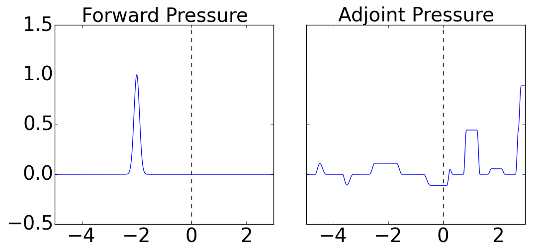
(a) Results for $t=0.0$ seconds.

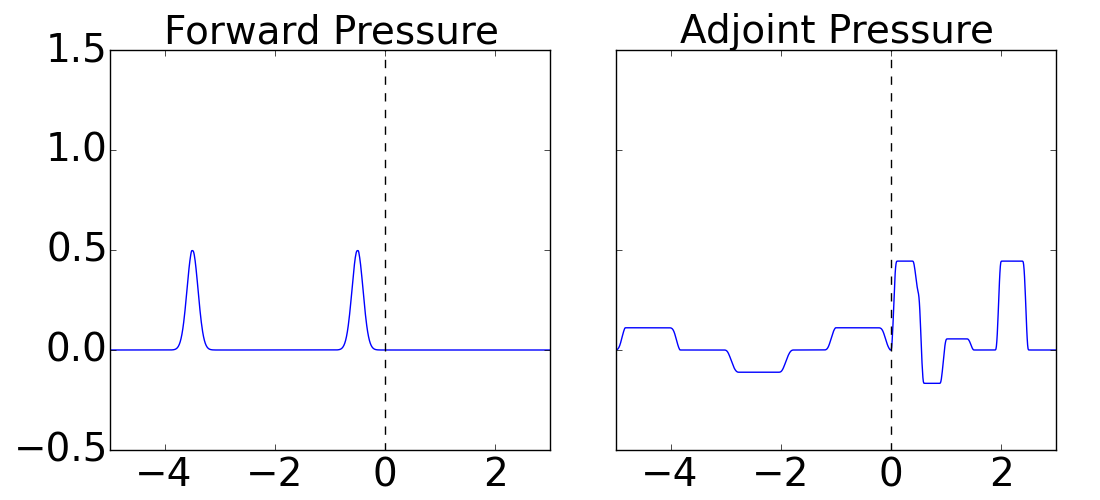
(b) Results for $t=1.5$ seconds.

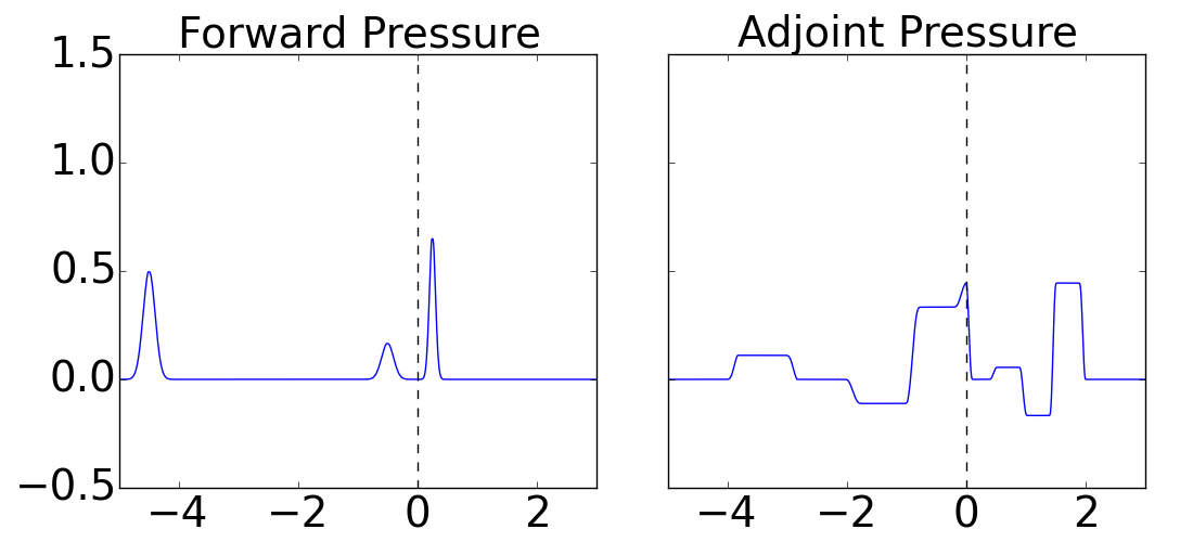
(c) Results for $t=2.5$ seconds.

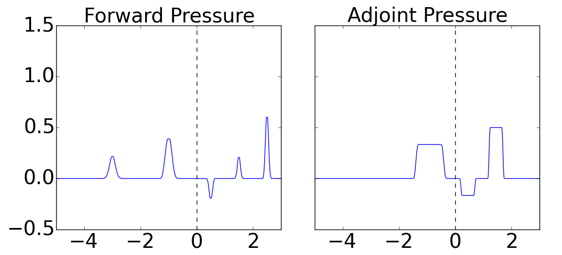
(d) Results for $t=15.0$ seconds.

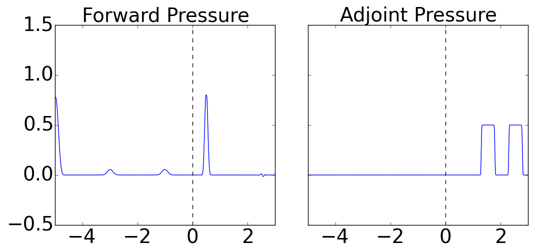
(e) Results for $t=19.0$ seconds.

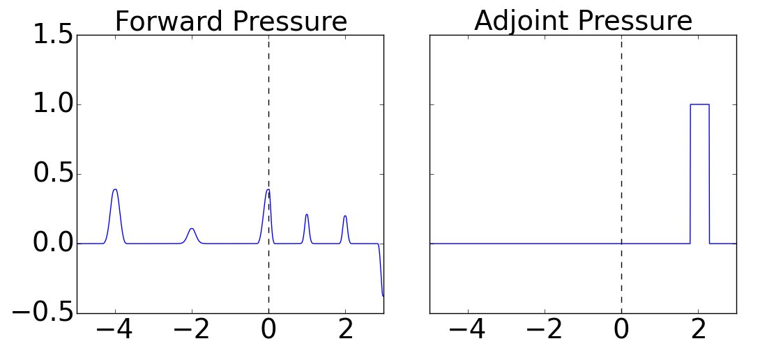
(f) Results for $t=20.0$ seconds.

Figure 1: Computed results for one-dimensional acoustics problem. The $y$-axis is the same for both plots in each subfigure. The adjoint pressure evolves backward in time from (f) to (a).

To better visualize how the waves are moving through the domain, it is helpful to look at the data in the $x$-$t$ plane as shown in Fig. 2(a). For Fig. 2(a), the horizontal axis is the position, $x$, and the vertical axis is time. The left plot shows in red the locations where the $1-$norm of $q(x,t)$ is greater than or equal to $0.1$. The right plot shows in blue the locations where the $1-$norm of $\hat{q}(x,t)$ is greater than or equal to $0.1$.

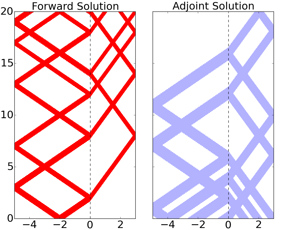
(a) The 1-norm of $q(x,t)$ and $\hat{q}(x,t)$ are shown in the left and right figures respectively, showing all waves.

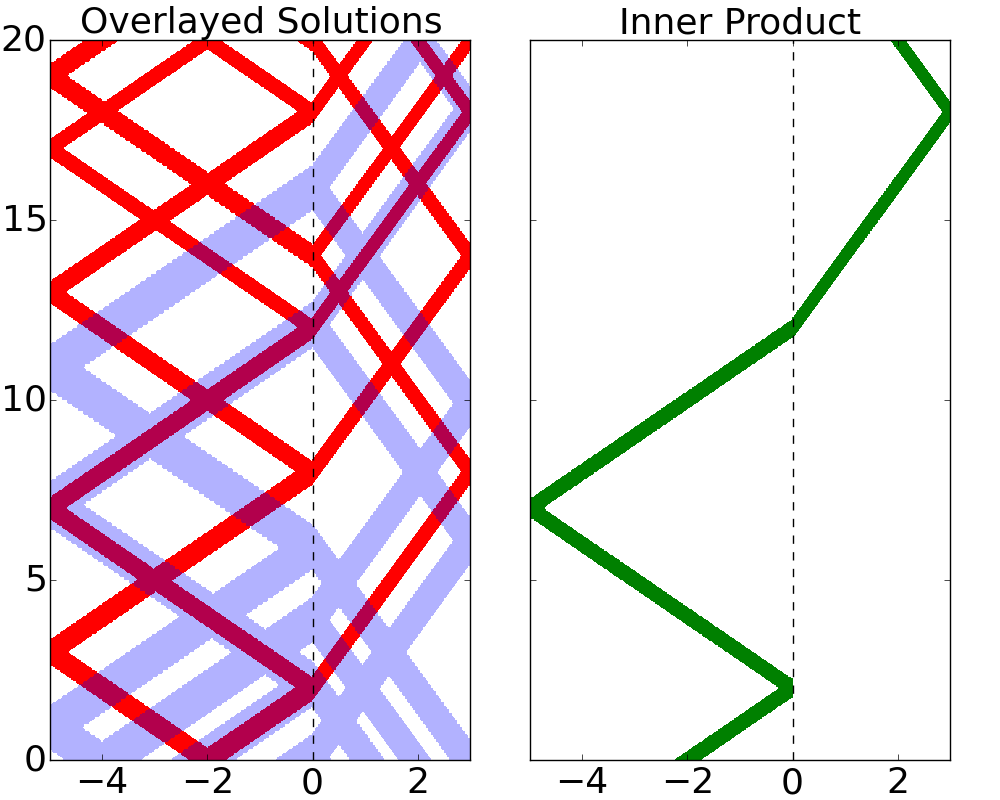
(b) The 1-norm of $q(x,t)$ and $\hat{q}(x,t)$ are overlayed in the left figure. Their inner product is shown in the right, indicating where the forward problem should be refined when only the solution $q(x,t)$ for $1.8<x<2.3$ at time $t=20$ is of interest.

Figure 2: Computed results for one-dimensional acoustics from Fig. 1, shown in the $x$-$t$ plane. The $y$-axis is the same for both plots in each subfigure.

5.1.1 Single Point In Time

Suppose that we are interested in the solution $q(x,t)$ in the region given by $1.8<x<2.3$ at the time $t=20$. We have already computed the adjoint solution, and have shown that by taking the inner product between the adjoint solution and the forward solution it is possible to identify the regions that will actually influence our region of interest at the final time. In the left side of Fig. 2(b) we have overlayed the forward and adjoint solutions, and viewing the data in the $x$-$t$ plane makes it fairly clear which parts of the wave from the forward solution actually effect our region of interest at the final time.

Figure 2(b) also shows, on the right, the locations where the inner product between the forward and adjoint solution is greater than or equal to 0.1 as time progresses. At each time step this is clearly identifying the regions in the computational domain that we are interested in. If we were using adaptive mesh refinement, these areas identified by where $\hat{q}^{T}(x,t)q(x,t)$ exceeds some tolerance are precisely the areas we would flag for refinement. Note that a mesh refinement strategy based on wherever the $1-$norm of $q(x,t)$ is large would result in refinement of many areas in the computational domain that will have no effect on our area of interest at the final time (all the red regions in the left plot of Fig. 2(a)).

5.1.2 Time Range

Suppose that we are interested in the accurate estimation of the pressure in the interval given by $1.8<x<2.3$ for the time range $t_{s}\leq t\leq t_{f}$, where $t_{s}=18$ and $t_{f}=20$. Define $\hat{q}(x,t;\overline{t})$ as the adjoint based on data $\hat{q}(x,\overline{t})=\varphi(x)$. Then for each $\hat{t}$ in the interval $[t_{s},t_{f}]$, we need to consider the inner product of $q(x,t)$ with $\hat{q}(x,t;\hat{t})$. Note that since the adjoint is autonomous in time, $\hat{q}(x,t;\hat{t})=\hat{q}(x,t_{f}-\hat{t}+t;t_{f})$. Therefore, we must consider the inner product

$$\hat{q}^{T}(x,t_{f}-\hat{t}+t;t_{f})q(x,t)$$

for $\hat{t}\in[t_{s},t_{f}]$. Since we are in fact only concerned when this inner product is greater than some tolerance, we can simply consider

$$\max\limits_{t_{s}\leq\hat{t}\leq t_{f}}\hat{q}^{T}(x,t_{f}-\hat{t}+t;t_{f})q(x,t)$$

and refine when this maximum inner product is above the given tolerance. Define $\tau=t_{f}-\hat{t}+t$. Then this maximum inner product can be rewritten as

$$\max\limits_{T\leq\tau\leq t}\hat{q}^{T}(x,\tau;t_{f})q(x,t)$$

where $T=\min(t+t_{f}-t_{s},~{}t_{f})$.

We now drop the cumbersum notation $\hat{q}(x,t;t_{f})$ in favor of the simpler $\hat{q}(x,t)$ with the understanding that the adjoint is based on the data $\hat{q}(x,t_{f})=\varphi(x)$. The left side of Fig. 3 shows in red the locations where the 1-norm of $q(x,t)$ is greater than or equal to 0.1 and in blue the locations where the 1-norm of $\hat{q}(x,\tau)$ is greater than or equal to 0.1, for $T\leq\tau\leq t$. Figure 3 also shows, on the right, the locations where the maximum inner product equation given above exceeds the tolerance of 0.1. At each time step this is clearly identifying the regions in the computational domain that will influence the interval of interest in the given time range. Therefore, the regions identified by this method are the regions that should be refined at each time step.

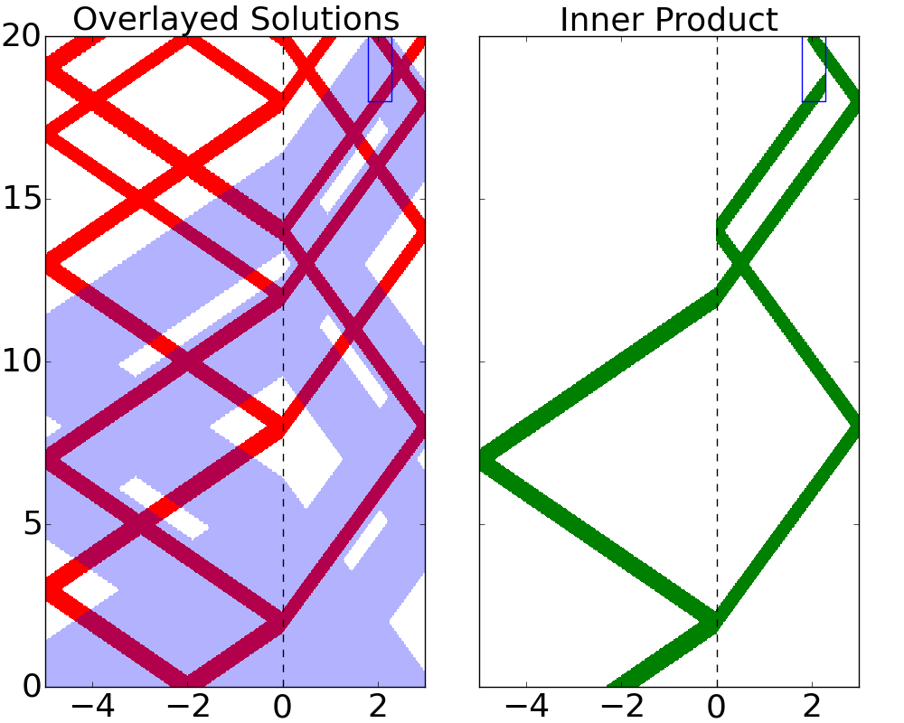
Figure 3: Computed results for one-dimensional acoustics in the case when the solution $q(x,t)$ for $1.8<x<2.3$ and $18\leq t\leq 20$ is of interest, as indicated by the box in each $x$–$t$ plot. Left: 1-norm for $q(x,t)$ and $\hat{q}(x,\tau)$ for $18\leq\tau\leq 20$. Right: Max inner product over the given time range, showing the additional wave that must be refined. The time axis is the same for both plots.

5.2 Acoustics in Two Space Dimensions

In two dimensions the linear acoustics equations are

$$p_{t}(x,y,t)+K(x,y)\left(u_{x}(x,y,t)+v(x,y,t)_{y}\right) =0 x\in[a,b],y\in[\alpha,\beta],t>t_{0}$$

$$\rho(x,y)u_{t}(x,y,t)+{p_{x}(x,y,t)} =0 x\in[a,b],y\in[\alpha,\beta],t>t_{0}$$

$$\rho(x,y)v_{t}(x,y,t)+{p_{y}(x,y,t)} =0 x\in[a,b],y\in[\alpha,\beta],t>t_{0}.$$

Setting

$$A(x,y)=\left[\begin{matrix}0&K&0\\ 1/\rho&0&0\\ 0&0&0\end{matrix}\right],\hskip 7.22743ptB(x,y)=\left[\begin{matrix}0&0&K\\ 0&0&0\\ 1/\rho&0&0\end{matrix}\right],\hskip 7.22743ptq(x,y,t)=\left[\begin{matrix}p\\ u\\ v\end{matrix}\right],$$

gives us the equation $q_{t}(x,y,t)+A(x,y)q_{x}(x,y,t)+B(x,y)q_{y}(x,y,t)=0$.

Suppose that we are interested in the accurate estimation of the pressure in the area defined by a square centered about $(x,y)=(3.56,0.56)$. Setting

$$J=2\int_{3.32}^{3.8}\int_{0.32}^{0.8}p(x,y,t_{f})dy\,dx,$$

the problem then requires that

(13) $$\varphi(x,y)=\left[\begin{matrix}2I(x,y)\\ 0\\ 0\end{matrix}\right],$$

where

(16) $$I(x,y)=\left\{\begin{array}[]{lr}1&\hskip 21.68121pt\textnormal{if }3.32\leq x\leq 3.8\textnormal{ and }0.32\leq y\leq 0.8,\\ 0&\textnormal{otherwise.}\end{array}\right.$$

Note that the coefficient of 2 in the definition of the functional $J$ is chosen for convenience. This coefficient can be chosen to be any value, provided that the refinement tolerance later on is adjusted accordingly. Define

$$\hat{q}(x,y,t_{f})=\left[\begin{matrix}\hat{p}(x,y,t_{f})\\ \hat{u}(x,y,t_{f})\\ \hat{v}(x,y,t_{f})\end{matrix}\right]=\varphi(x,y),$$

and note that for any time $t_{0}<t_{f}$ we have

$$\int_{t_{0}}^{t_{f}}\int_{a}^{b}\int_{\alpha}^{\beta}\hat{q}^{T}\left(q_{t}+A(x,y)q_{x}+B(x,y)q_{y}\right)dy\,dx\,dt=0.$$

Integrating by parts yields the equation

$$\left.\int_{a}^{b}\int_{\alpha}^{\beta}\hat{q}^{T}q\,dy\,dx\right|^{t_{f}}_{t_{0}} +\left.\int_{t_{0}}^{t_{f}}\int_{\alpha}^{\beta}\hat{q}^{T}A(x,y)q\,dy\,dt\right|^{b}_{a}+\left.\int_{t_{0}}^{t_{f}}\int_{a}^{b}\hat{q}^{T}B(x,y)q\,dx\,dt\right|^{\beta}_{\alpha}$$

(17) $$- \int_{t_{0}}^{t_{f}}\int_{a}^{b}\int_{\alpha}^{\beta}q^{T}\left(\hat{q}_{t}+\left(A^{T}(x,y)\hat{q}\right)_{x}+\left(B^{T}(x,y)\hat{q}\right)_{y}\right)dy\,dx\,dt=0.$$

Note that if we can define an adjoint problem such that all but the first term in this equation vanishes then we are left with

$$\int_{a}^{b}\int_{\alpha}^{\beta}\hat{q}^{T}(x,y,t_{f})q(x,y,t_{f})dy\,dx=\int_{a}^{b}\int_{\alpha}^{\beta}\hat{q}^{T}(x,y,t_{0})q(x,y,t_{0})dy\,dx,$$

which is the expression that allows us to use the inner product of the adjoint and forward problems at each time step to determine what regions will influence the point of interest at the final time. The adjoint problem required to accomplish this depends on the boundary conditions of the forward problem in question. Two different boundary conditions for the forward problem and the corresponding adjoint problems are discussed further below.

As an example, consider $t_{0}=0$, $a=-4$, $b=8$, $\alpha=-1$, $\beta=11$, $K=4$ and $\rho=1$. As initial data for $q(x,y,t)$ we take a smooth radially symmetric hump in pressure, and a zero velocity in both $x$ and $y$ directions. The initial hump in pressure is given by

(20) $$p(x,y,0)=\left\{\begin{array}[]{lr}3+\cos\left((\pi\left(r-0.5\right)/w\right)&\hskip 21.68121pt\textnormal{if }\left|r-0.3\right|\leq w,\\ 0&\textnormal{otherwise.}\end{array}\right.$$

with $w=0.15$ and $r=\sqrt{\left(x-0.5\right)^{2}+\left(y-1\right)^{2}}$. As time progresses, this hump in pressure will radiate outward symmetrically.

Since the time interval of interest is given by $t_{s}\leq t\leq t_{f}$, at time $t$ we will refine the computational mesh where

$$\max\limits_{T\leq\tau\leq t}\hat{q}^{T}(x,y,\tau)q(x,y,t)$$

is above some tolerance, with $T=\min(t+t_{f}-t_{s},0)$. For the examples below this tolerance is set to $0.02$.

Note that adaptive mesh refinement was used for the forward problem in these three examples, and the black outlines in each figure are the edges of different refinement levels. In each example, three levels of refinement are allowed for the forward problem, with a refinement ratio of 2 from each grid to the next. The adjoint problems were solved on a $50\times 50$ grid with no mesh refinement, which is also the resolution of the coarsest level for the forward problems.

5.2.1 Wall boundary conditions for a time point of interest

Suppose that $t_{f}=1.5$ seconds and that we are interested in the accurate calculation of the pressure only at the final time (so $t_{s}=t_{f}=1.5$). If we have the boundary conditions

$$u(a,y,t)=0,\hskip 7.22743ptu(b,y,t)=0 t\geq 0,$$

(21) $$v(x,\alpha,t)=0,\hskip 7.22743ptv(x,\beta,t)=0 t\geq 0,$$

then all but the first term in Equation Eq. 17 vanish if we define the adjoint problem

$$\hat{q}_{t}+\left(A^{T}(x,y)\hat{q}\right)_{x}+\left(B^{T}(x,y)\hat{q}\right)_{y}=0 x\in[a,b],y\in[\alpha,\beta],t>0$$

(22) $$\hat{u}(a,y,t)=0,\hskip 7.22743pt\hat{u}(b,y,t)=0 t\geq 0$$

$$\hat{v}(x,\alpha,t)=0,\hskip 7.22743pt\hat{v}(x,\beta,t)=0 t\geq 0.$$

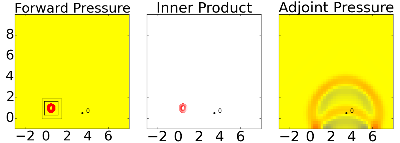
(a) Results at $t=0$.

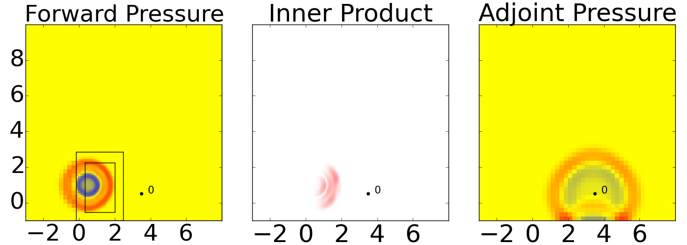
(b) Results at $t=0.5$.

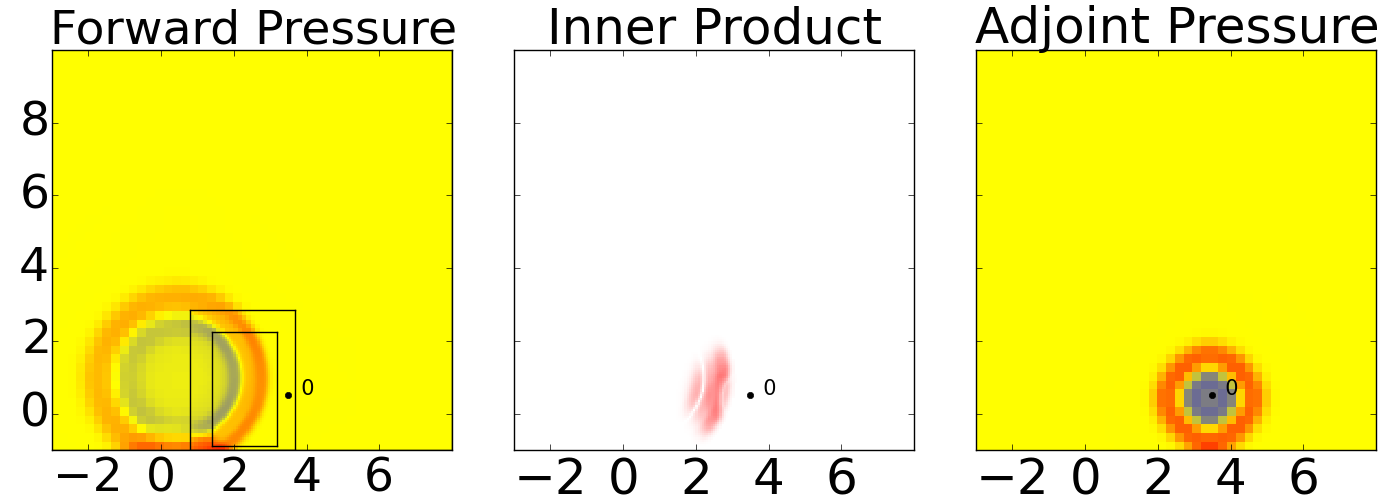
(c) Results at $t=1.0$.

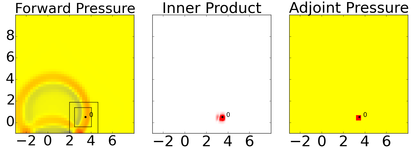
(d) Results at $t=1.5$.

Figure 4: Pressure for the two-dimensional acoustics problem with zero boundary conditions when only the pressure over the small region shown by the red square in the adjoint pressure plot at the final time t = 1.5 is of interest. The color scale for both pressure figures goes from blue to red, and ranges between $-1.0$ and 1.0 for the forward pressure and between $-0.25$ and 0.25 for the adjoint pressure. The color scale for the inner product figure goes from white to red, and ranges between 0 and 0.25. The $y$-axis is the same for all plots in each subfigure.

As the initial data for the adjoint $\hat{q}(x,y,t_{f})=\varphi(x,y)$ we have a square pulse in pressure, which was described in Equations Eq. 13 and Eq. 16. As time progresses backwards, waves radiates outward and reflect off the walls. As the initial data for $q(x,y,t)$ we have $q(x,y,0)=\left[p(x,y,0),0,0\right]^{T}$ where $p(x,y,0)$ is given in Equation Eq. 20.

Fig. 4 shows the Clawpack results for the pressure for both the forward and adjoint solutions at various times, as well as the inner product between the two. Here it is easy to see that the refinement is occurring where the inner product is large, and how the interaction between the forward and adjoint problems at each time step is generating the inner product.

5.2.2 Wall boundary conditions for a time range of interest

Now suppose that $t_{f}=6$ seconds, and that we are interested in the accurate calculation of the pressure over the time interval $1.0\leq t\leq 6.0$ (so, $t_{s}=1$ second). As in the previous example, consider wall boundary conditions Eq. 21. Then all but the first term in Equation Eq. 17 vanish if we define the adjoint problem Eq. 22.

(a) $t=0.0$

(b) $t=2.7$

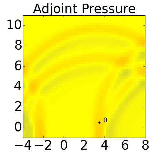
(c) $t=4.5$

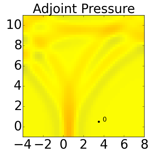
(d) $t=6.0$

Figure 5: Pressure for the two-dimensional acoustics adjoint problem with zero boundary conditions. Results are for the shown times given in seconds before the final time, since the “initial” conditions are given at the final time. The color scale goes from blue to red, and ranges between -0.3 and 0.3.

(a) Results at $t=0.0$ seconds.

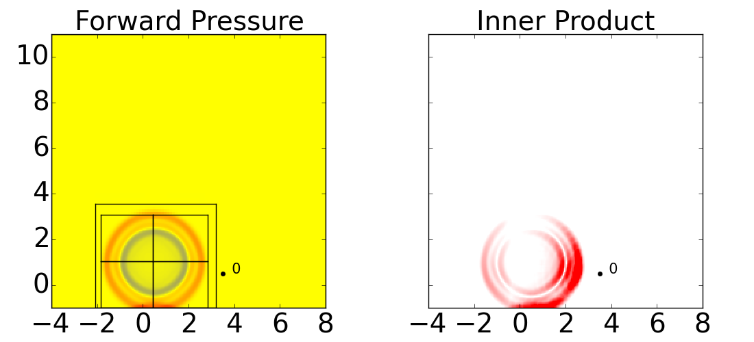
(b) Results at $t=0.9$ seconds.

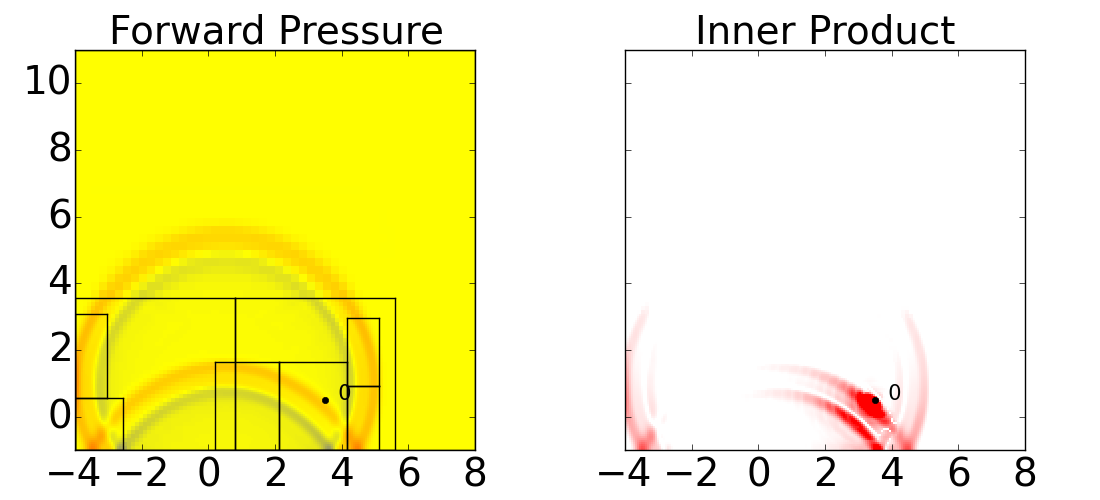
(c) Results at $t=2.1$ seconds.

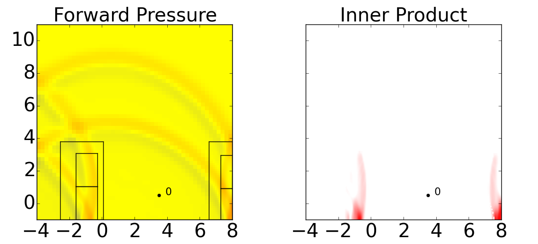
(d) Results at $t=3.9$ seconds.

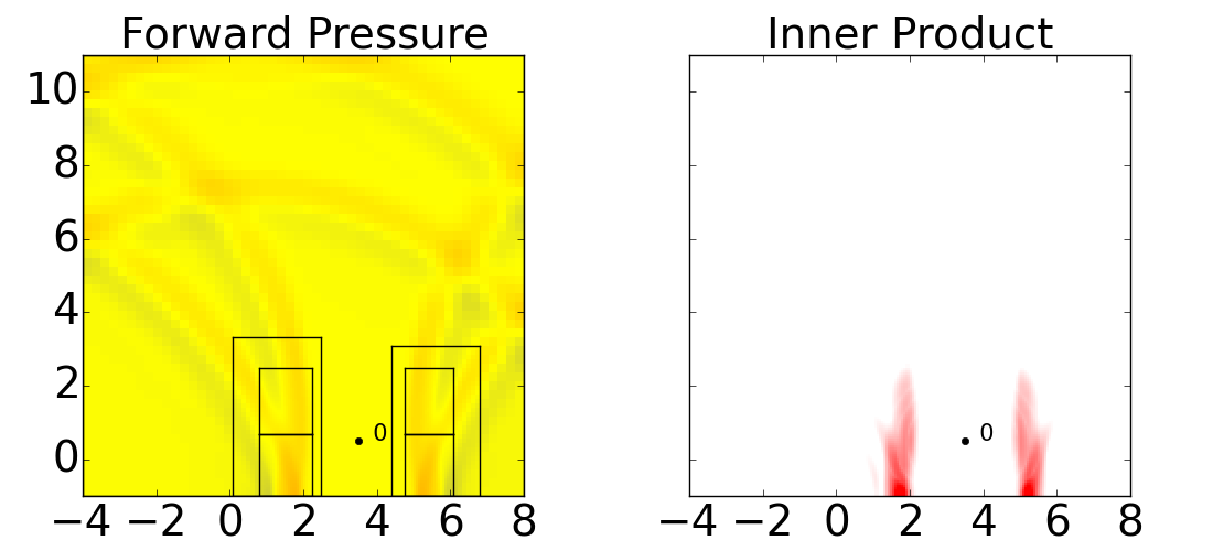
(e) Results at $t=5.1$ seconds.

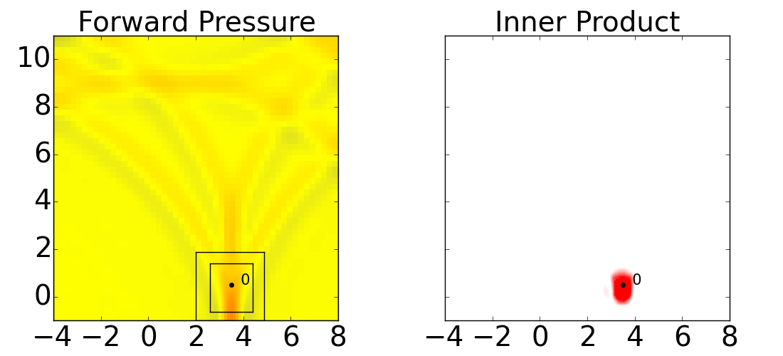
(f) Results at $t=6.0$ seconds.

Figure 6: Computed results for two-dimensional acoustics forward problem with zero boundary conditions. The $y$-axis is the same for both plots in each subfigure. The color scale for the pressure figures goes from blue to red, and ranges between $-1.5$ and 1.5. The color scale for the inner product figures goes from white to red, and ranges between 0.01 and 0.12.

Using the same initial conditions at in the previous example, Fig. 5 shows the Clawpack results for the adjoint pressure, $\hat{p}(x,y,t)$, at four different times. Again, as the initial data for $q(x,y,t)$ we have $q(x,y,0)=\left[p(x,y,0),0,0\right]^{T}$ where $p(x,y,0)$ is given in Equation Eq. 20. To more easily visualize which areas of the computational domain should be refined at each time step, it is helpful to consider the maximum inner product over the appropriate time range,

$$\max\limits_{T\leq\tau\leq t}\hat{q}^{T}(x,y,\tau)q(x,y,t),$$

with $T=\min(t+t_{f}-t_{s},0)$. Recall that the areas where this is large are the areas where adaptive mesh refinement should take place. Fig. 6 shows the Clawpack results for the pressure, $p(x,y,t)$, at six different times, along with this maximum inner product.

5.2.3 Mixed boundary conditions for a time range of interest

Now suppose one of the boundaries has outflow or non-reflecting boundary conditions, e.g. at $x=a$. The assumtion in this case is that this is an artificial computational boundary and ideally we would be solving a problem with no boundary at this edge. In other words we are assuming that if we were to solve the problem on a larger domain, extended for $x<a$, then waves that pass $x=a$ will not give rise to reflections that re-enter the computational domain. If we now consider the adjoint equation on the hypothetical extended domain, it is clear that waves in the adjoint solution should also pass through the computational boundary at $x=a$. Hence non-reflecting boundary conditions are the correct conditions to impose on the adjoint solution at any boundary where non-reflecting boundaries are assumed for the forward problem.

Using the same initial conditions and values for $t_{s}$ and $t_{f}$ as in the previous example, we now replace the boundary conditions at $x=a$ and $y=\beta$ by outflow boundary conditions to illustrate this. Figure 7 shows the Clawpack results for the pressure, $\hat{p}(x,y,t)$, at four different times. Fig. 8 shows the Clawpack results for the pressure, $p(x,y,t)$, at six different times, along with the maximum inner product in the appropriate time range.

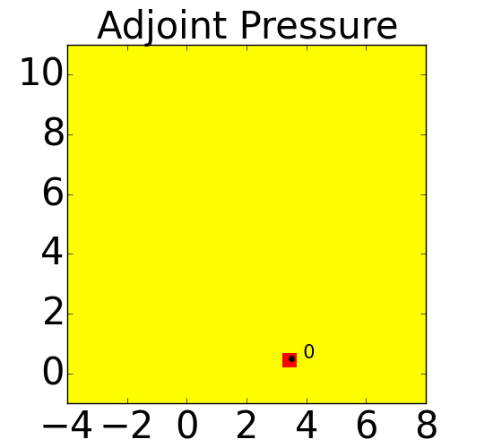
(a) $t=0.0$

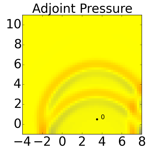
(b) $t=2.7$

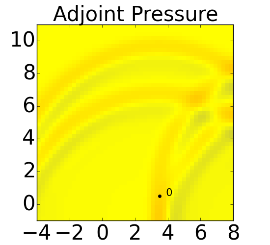
(c) $t=4.5$

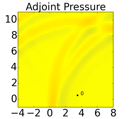
(d) $t=6.0$

Figure 7: Pressure for the two-dimensional acoustics adjoint problem with zero boundary conditions at $x=b$ and $y=\alpha$, and outflow boundary conditions at $x=a$ and $y=\beta$. Results are for the shown times given in seconds before the final time, since the “initial” conditions are given at the final time. The color scale goes from blue to red, and ranges between $-0.3$ and 0.3.

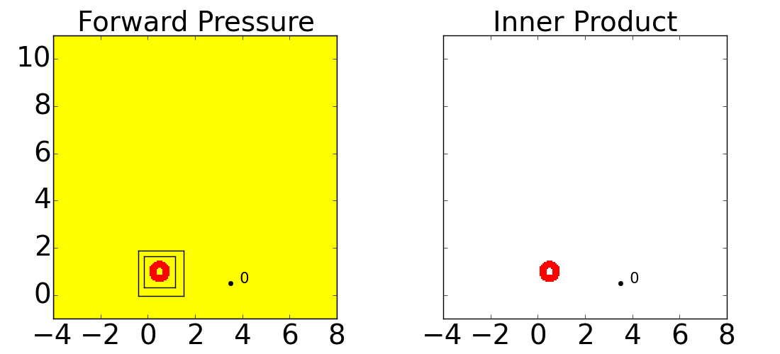
(a) Results at $t=0.0$ seconds.

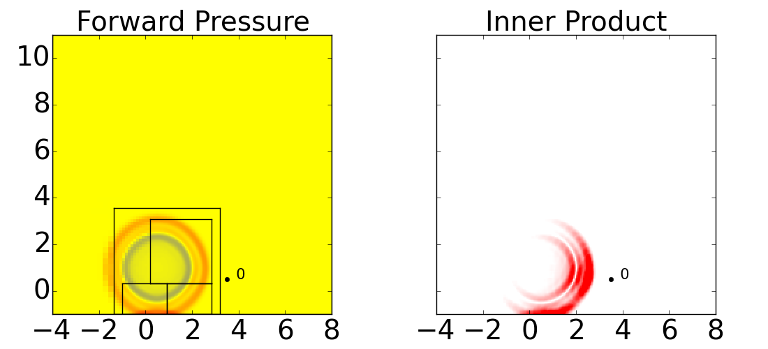
(b) Results at $t=0.9$ seconds.

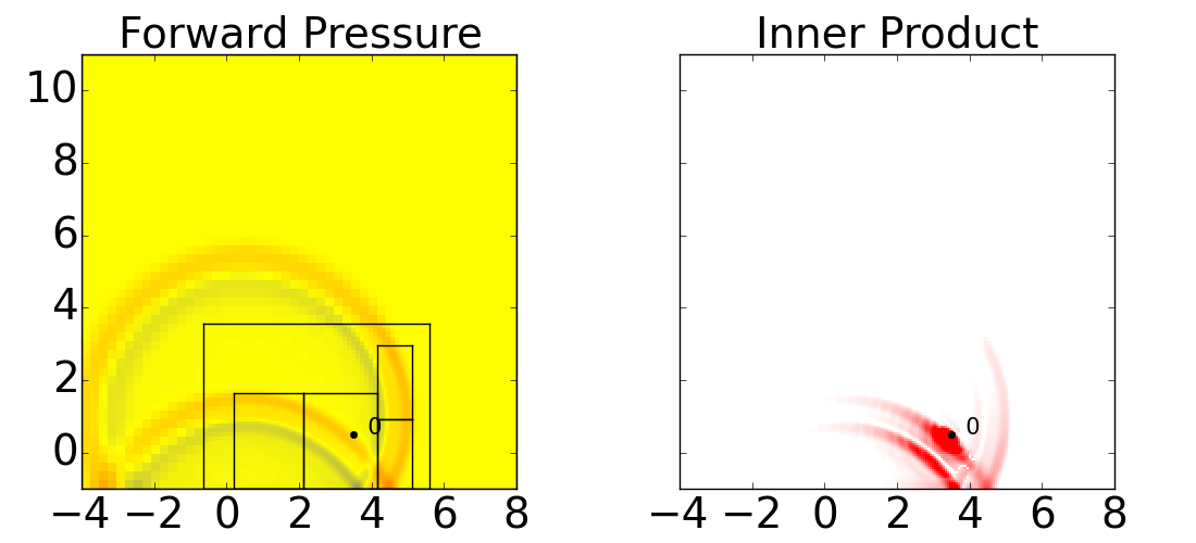
(c) Results at $t=2.1$ seconds.

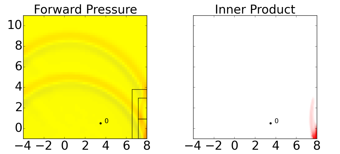
(d) Results at $t=3.9$ seconds.

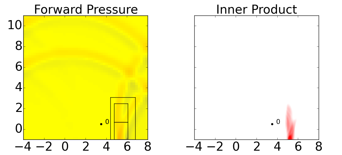
(e) Results at $t=5.1$ seconds.

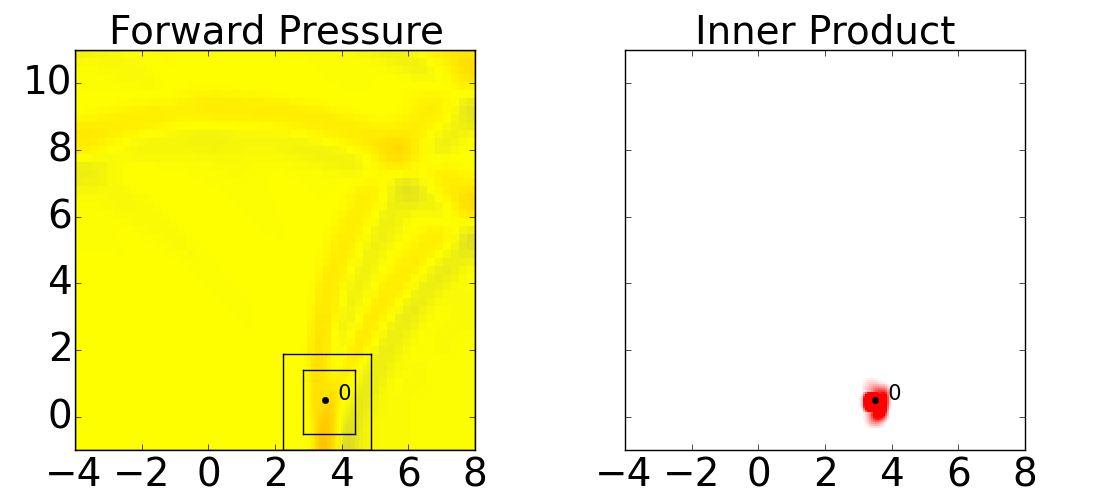
(f) Results at $t=6.0$ seconds.

Figure 8: Computed results for two-dimensional acoustics forward problem with zero boundary conditions at $x=b$ and $y=\alpha$, and outflow boundary conditions at $x=a$ and $y=\beta$. The $y$-axis is the same for both plots in each subfigure. The color scale for the pressure figures goes from blue to red, and ranges between $-1.5$ and 1.5. The color scale for the inner product figures goes from white to red, and ranges between 0.01 and 0.12. Compare this to Fig. 6, where we were refining around two waves converging on the gauge.

5.2.4 Computational Performance

All of the above examples were run on a laptop, and the same examples utilizing the standard AMR flagging techniques were also run for timing comparisons.

For the acoustics examples, the standard refinement technique in AMRClaw computes the spatial difference in each direction and for each component of $q$ and flags any points where this is greater than some tolerance. We will refer to this flagging technique as pressure-flagging. In contrast, for the adjoint refinement technique we are computing the inner product between $\hat{q}$ and $q$, where the times at which each of these is evaluated are problem specific, and flagging any point where this inner product is greater than some tolerance. We will refer to this flagging technique as adjoint-flagging.

Table 1: Timing comparison for the examples in Section 5.2 given in seconds.

		Adjoint-Flagging
Example	Pressure-Flagging	Forward	Adjoint
Section 5.2.1	3.137	1.325	0.465
Section 5.2.2	15.664	6.866	0.683
Section 5.2.3	13.504	5.492	0.666

For these examples, the tolerance for pressure-flagging is set to 0.1 and the tolerance for the adjoint-flagging is set to 0.02. The timing results for these examples is shown in Table 1. In the table, the timings in the “Pressure-Flagging” column refer to the time required when utilizing the pressure-flagging techniques available in AMRClaw, the timings in the “Forward” column refer to the time required to solve the problem when utilizing the adjoint-flagging method, and the timings in the “Adjoint” column refer to the time required to solve the adjoint equations. Note that the adjoint-flagging method does require solving two different problems, but the total computational time required is still significantly less than the time required for the original refinement method.

Another consideration when comparing the adjoint-flagging method with the pressure-flagging method already in place in AMRClaw is the accuracy of the results. To test this, a gauge was placed in each example and the output at that gauge compared across the different methods.

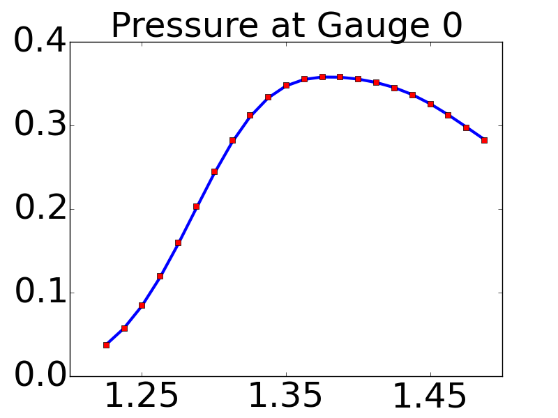
(a) From example in Section 5.2.1

(b) From example in Section 5.2.2

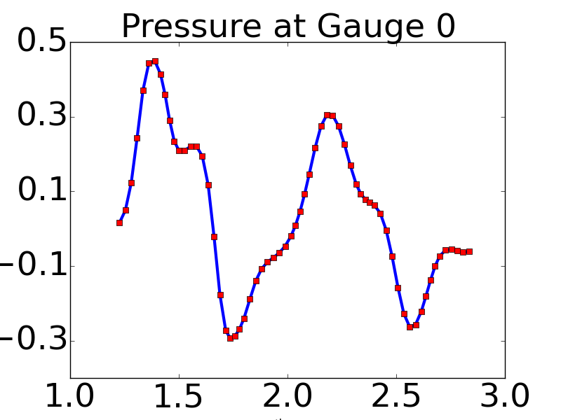
(c) From example in Section 5.2.3

Figure 9: Overlaid gauge results for acoustics problems using the original and adjoint refinement methods. Results for the original pressure-flagging refinement method are shown in red squares, and the results for the adjoint refinement method are shown in the blue lines. Along the $x$-axis, the time since the beginning of the simulation is shown in seconds.

In the acoustics examples the gauge was placed at the center of the region of interest: $(x,y)=(3.5,0.5)$, and is shown as a black dot in each of the two dimensional acoustics figures previously shown. In Fig. 9 the gauge results from the adjoint-flagging method are shown as a blue line and then the results from the pressure-flagging method were overlaid in red squares. Note that the two outputs are indistinguishable for all three examples, indicating that the use of the adjoint method did not have a significant detrimental impact on the accuracy of the calculated results.

5.3 Tsunami Modeling

Blaise et al. [10] present a method to reconstruct the tsunami source using a discrete adjoint approach. In this work we focus on the problem of efficiently solving the shallow water equations once the initial water displacement is known, and discretize the continuous adjoint for the linearized shallow water equations. The goal is to identify waves propagating over the ocean that must be accurately tracked because they will reach a point of interest on the coast, which is otherwise difficult to automate for reasons mentioned in the introduction.

The algorithms used in GeoClaw for tsunami modeling are described in detail in [23], and in general solve the two-dimensional nonlinear shallow water equations

(23) $$h_{t}+(hu)_{x}+(hv)_{y} =0,$$

(24) $$(hu)_{t}+(hu^{2}+\tfrac{1}{2}gh^{2})_{x}+(huv)_{y} =-ghB_{x},$$

(25) $$(hv)_{t}+(huv)_{x}+(hv^{2}+\tfrac{1}{2}gh^{2})_{y} =-ghB_{y},$$

where $u(x,y,t)$ and $v(x,y,t)$ are the depth-averaged velocities in the two horizontal directions, $B(x,y,t)$ is the topography, $g$ is the gravitational constant, and $h(x,y,t)$ is the fluid depth. We will use $\eta(x,y,t)$ to denote the water surface elevation,

$$\eta(x,y,t)=h(x,y,t)+B(x,y,t),$$

$\mu=hu$ to denote the momentum in the $x$ direction, and $\gamma=hv$ to denote the momentum in the $y$ direction.

As initial data, we consider a source model for the 1964 Alaska earthquake, which generated a tsunami that affected the entire Pacific Ocean. The major waves impinging on Crescent City, California from this tsunami all occurred within 11 hours after the earthquake, so simulations will be run to this time. To simulate the effects of this tsunami on Crescent City a coarse grid is used over the entire Pacific (1 degree resolution) where the ocean is at rest. In addition to AMR being used to track propagating waves on finer grids, higher levels of refinement are allowed or enforced around Crescent City when the tsunami arrives. A total of 4 levels of refinement are used, starting with 1-degree resolution on the coarsest level, and with refinement ratios of 5, 6, and 6 from one level to the next. Only 3 levels were allowed over most of the Pacific, and the remaining level was used over the region around Crescent City. Level 4, with 20-second resolution, is still too coarse to provide any real detail on the effect of the tsunami on the harbor. It does, however, allow for a comparison of flagging cells for refinement using the adjoint method and using the default method implemented in Geoclaw.

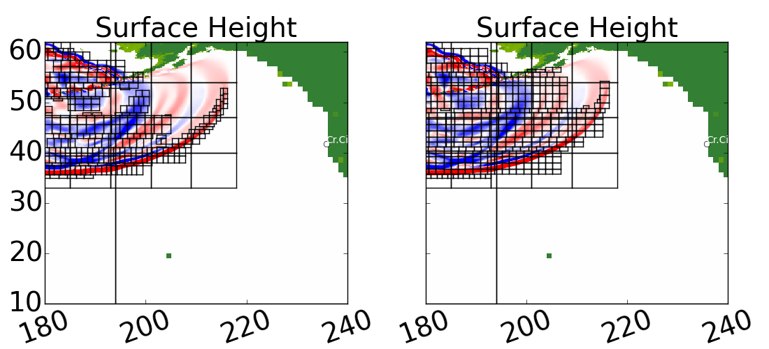
(a) Results 2 hours after the earthquake.

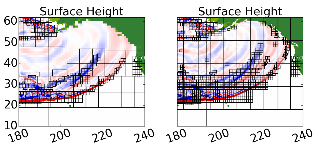
(b) Results 4 hours after the earthquake.

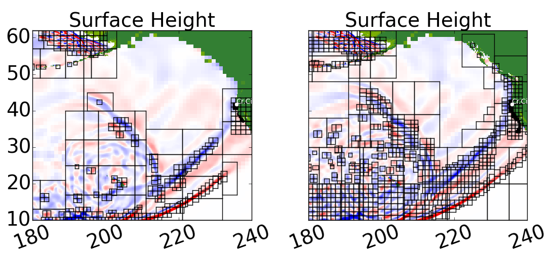
(c) Results 6 hours after the earthquake.

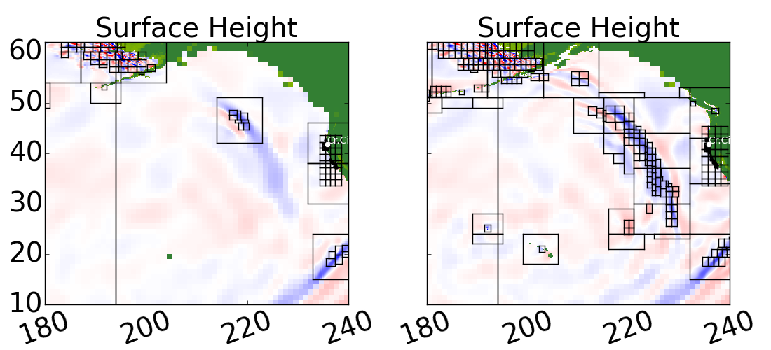
(d) Results 8 hours after the earthquake.

Figure 10: Computed results for tsunami propagation problem on two different runs utilizing the surface-flagging technique. The $y$-axis is the same for both plots in each subfigure. In each subfigure the left shows results for a tolerance of $0.14$ and the right shows results for a tolerance of $0.09$. The color scale goes from blue to red, and ranges between $-0.3$ and 0.3 meters (surface elevation relative to sea level). Rectangles show patches of up to 60 $\times$ 60 grid cells.

The default Geoclaw refinement technique flags cells for refinement when the elevation of the sea surface relative to sea level is above some set tolerance [23]. We will refer to this flagging method as surface-flagging. The value selected for this tolerance has a significant impact in the results calculated by the simulation, since a smaller tolerance will result in more cells being flagged for refinement. Consequently, a smaller tolerance both increases the simulation time required and theoretically increases the accuracy of the results.

Two Geoclaw simulations were preformed using surface-flagging, one with a tolerance of $0.14$ and another with a tolerance of $0.09$. Fig. 10 shows the results of these two simulations side by side for the sake of comparison. Recalling that the black outlines in each figure are the edges of grid patches at different refinement levels, it is easy to see that as expected the simulation with the smaller tolerance flagged more cells for refinement. Note that the simulation with a surface-flagging tolerance of $0.14$ continues to refine the first wave until it arrives at Crescent City about 5 hours after the earthquake, but after about 6 hours stops refining the main secondary wave which reflects off the Northwestern Hawaiian (Leeward) Island chain before heading towards Crescent City. The second simulation, with a surface-flagging tolerance of $0.09$ continues to refine this secondary wave until it arrives at Crescent City.

These two tolerances were selected because they are illustrative of two constraints that typically drive a Geoclaw simulation. The larger surface-flagging tolerance, of $0.14$, is approximately the largest tolerance that will refine the initial wave until it reaches Crescent City. Therefore, it essentially corresponds to a lower limit on the time required: any Geoclaw simulation with a larger surface-flagging tolerance would run more quickly but would fail to give accurate results for even the first wave. Note that for this particular example, even when the simulation will only give accurate results for the first wave to reach Crescent City, a large area of the wave front that is not headed directly towards Crescent City is being refined with the AMR. The smaller surface-flagging tolerance, of $0.09$, refines all of the waves of interest that impinge on Crescent City thereby giving more accurate results at the expense of longer computational time.

Now we consider the adjoint approach, which will allow us to refine only those sections of the wave that will affect our target region. The linearized shallow water equations govern waves with small-amplitude relative to the fluid depth. In the case of ocean waves, the nonlinear effects become significant when a wave approaches a shore line. Since the water depth in the adjoint solution is only used to identify areas of interest, high order accuracy is not necessary. Furthermore, computational efficiency is the driving force behind our implementation of the adjoint method. Therefore, we have solved the simpler linearized equations for the adjoint problem. However, the algorithms for the nonlinear equations already implemented in GeoClaw are still utilized for the forward problem (albeit with a variant of the Roe approximate Riemann solver [16] that amounts to a local linearization at each cell edge).

To find the adjoint problem for the linearized equations, we begin by letting $(\mu,\gamma)=(hu,hv)$ represent the momentum and noting that the two momentum equations from Eq. 23 can be rewritten as

$$\mu_{t}+(hu^{2})_{x}+gh(h+B)_{x}+(huv)_{y} =0,$$

$$\gamma_{t}+(huv)_{x}+(hv^{2})_{y}+gh(h+B)_{y} =0.$$

Linearizing these equations as well as the continuity equation about a flat surface $\bar{\eta}$ and zero velocity $\bar{u}=0$, with $\bar{h}(x,y)=\bar{\eta}-B(x,y)$ gives

$$\tilde{\eta}_{t}+\tilde{\mu}_{x}+\tilde{\gamma}_{y} =0$$

$$\tilde{\mu}_{t}+g\bar{h}(x,y)\tilde{\eta}_{x} =0$$

$$\tilde{\gamma}_{t}+g\bar{h}(x,y)\tilde{\eta}_{y} =0$$

for the perturbation $(\tilde{\eta},\tilde{\mu},\tilde{\gamma})$ about $(\bar{\eta},0,0)$. Dropping tildes and setting

$$A(x,y)=\left[\begin{matrix}0&1&0\\ g\bar{h}(x,y)&0&0\\ 0&0&0\end{matrix}\right],\hskip 7.22743ptB(x,y)=\left[\begin{matrix}0&0&1\\ 0&0&0\\ g\bar{h}(x,y)&0&0\end{matrix}\right],\hskip 7.22743ptq(x,y,t)=\left[\begin{matrix}\eta\\ \mu\\ \gamma\end{matrix}\right],$$

gives us the system $q_{t}(x,y,t)+A(x,y)q_{x}(x,y,t)+B(x,y)q_{y}(x,y,t)=0$.

For this example, we are interested in the accurate calculation of the water surface height in the area about Crescent City, California. To focus on this area, we define a circle of radius $1^{\circ}$ centered about $(x_{c},y_{c})=(235.80917,41.74111)$ where $x$ and $y$ are being measured in degrees. Setting

$$J=4\int_{x_{min}}^{x_{max}}\int_{y_{min}(x)}^{y_{max}(x)}\eta(x,y,t_{f})dy\,dx,$$

where the limits of integration define the appropriate circle, the problem then requires that

(26) $$\varphi(x,y)=\left[\begin{matrix}I(x,y)\\ 0\\ 0\end{matrix}\right],$$

where

(29) $$I(x,y)=\left\{\begin{array}[]{ll}1&\hskip 21.68121pt\textnormal{if~{}}\sqrt{\left(x-x_{c}\right)^{2}+\left(y-y_{c}\right)^{2}}\leq 1,\\ 0&\hskip 21.68121pt\textnormal{otherwise.}\end{array}\right.$$

Define

$$\hat{q}(x,y,t_{f})=\left[\begin{matrix}\hat{\eta}(x,y,t_{f})\\ \hat{\mu}(x,y,t_{f})\\ \hat{\gamma}(x,y,t_{f})\end{matrix}\right]=\varphi(x,y),$$

and note that

$$\int_{t_{0}}^{t_{f}}\int_{a}^{b}\int_{\alpha}^{\beta}\hat{q}^{T}\left(q_{t}+A(x,y)q_{x}+B(x,y)q_{y}\right)dy\,dx\,dt=0.$$

Again, integrating by parts yields the equation Eq. 17 and the adjoint equation has the form

(30) $$\hat{q}_{t}+\left(A^{T}(x,y)\hat{q}\right)_{x}+\left(B^{T}(x,y)\hat{q}\right)_{y}=0.$$

We require this to hold in the same domain as the forward problem, while also imposing a coastline and boundary conditions similar to those that constrained the forward problem.

The topography files used for the adjoint problem are the same as those used for the forward problem. However, given that the adjoint problem is being solved on a coarser grid than the forward problem, the coastline between the two simulations varies. Internally, GeoClaw constructs a piecewise-bilinear function from the union of any provided topography files. This function is then integrated over computational grid cells to obtain a single topography value in each grid cell. Note that this means that the topography used in finer cells for the forward problem has an average value that is equal to the corresponding coarse cell value in the adjoint problem. Since the coastline varies between the two simulations, when computing the inner product it is possible to find grid cells that are wet in the forward solution and dry in the adjoint solution. In this case, the inner product in those grid cells is set to zero.

The boundary conditions at the coastline also vary slightly between the forward and adjoint problems. The solution of the forward problem involved using a variant of the Roe approximate Riemann solver [16], which allows for a changing coastline due to inundation. For our simplified solution of the linearized adjoint equation, we assume wall boundary conditions (zero normal velocity) at the interfaces between any wet cell and dry cell.

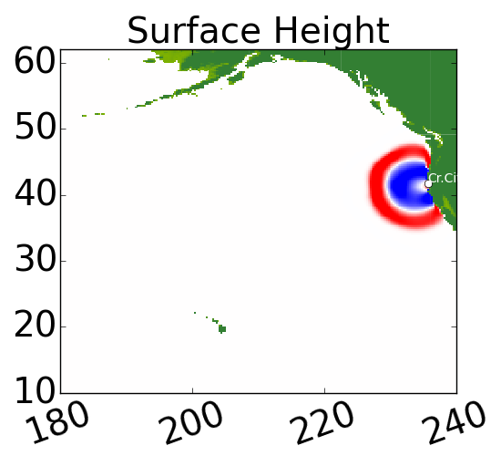
(a) 1 hour

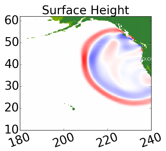
(b) 3 hours

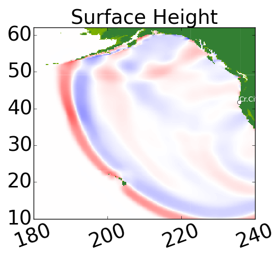
(c) 5 hours

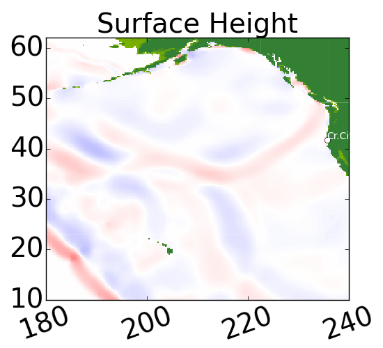
(d) 7 hours

Figure 11: Computed results for tsunami propagation adjoint problem. Times shown are the number of hours before the final time, since the “initial” conditions are given at the final time. The color scale goes from blue to red, and ranges between $-0.05$ and $0.05$.

As the initial data for the adjoint $\hat{q}(x,y,t_{f})=\varphi(x,y)$ we have a circular area with elevated water height as described in equations Eq. 26 and Eq. 29. Fig. 11 shows the results for the simulation of this adjoint problem. For this simulation a grid with 15 arcminute $=0.25^{\circ}$ resolution was used over the entire Pacific and no grid refinement was allowed. The simulation was run out to 11 hours.

The simulation of this tsunami using adjoint-flagging for the AMR was run using the same initial grid over the Pacific, the same refinement ratios, and the same initial water displacement as our previous surface-flagging simulation. The only difference between this simulation and the previous one is the flagging technique utilized. The first waves arrive at Crescent City around 4 hours after the earthquake, so we set $t_{s}=3.5$ hours and $t_{f}=11$ hours. Recall that the areas where the maximum inner product over the appropriate time range,

$$\max\limits_{T\leq\tau\leq t}\hat{q}^{T}(x,y,\tau)q(x,y,t)$$

with $T=\min(t+t_{f}-t_{s},0)$, is large are the areas where adaptive mesh refinement should take place.

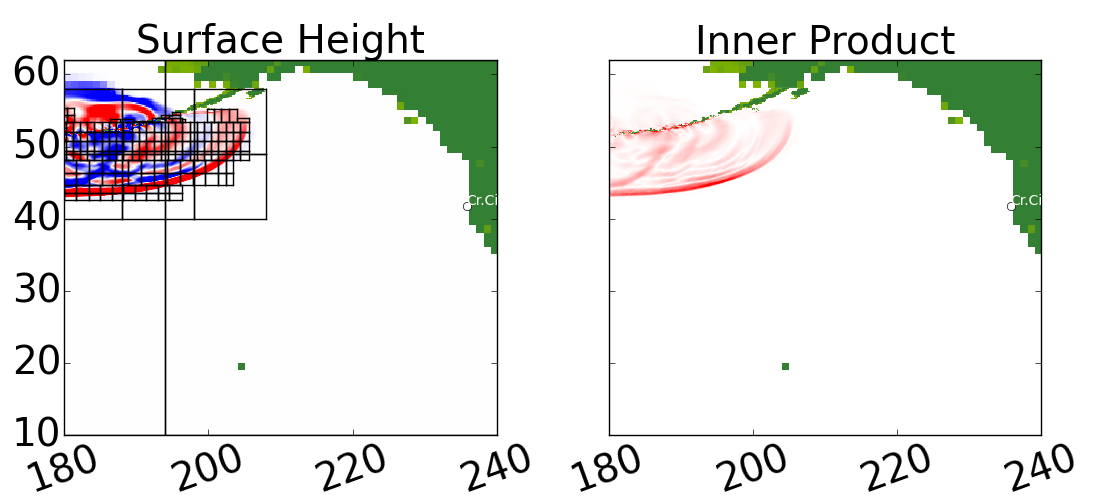
(a) Results 1 hour after the earthquake.

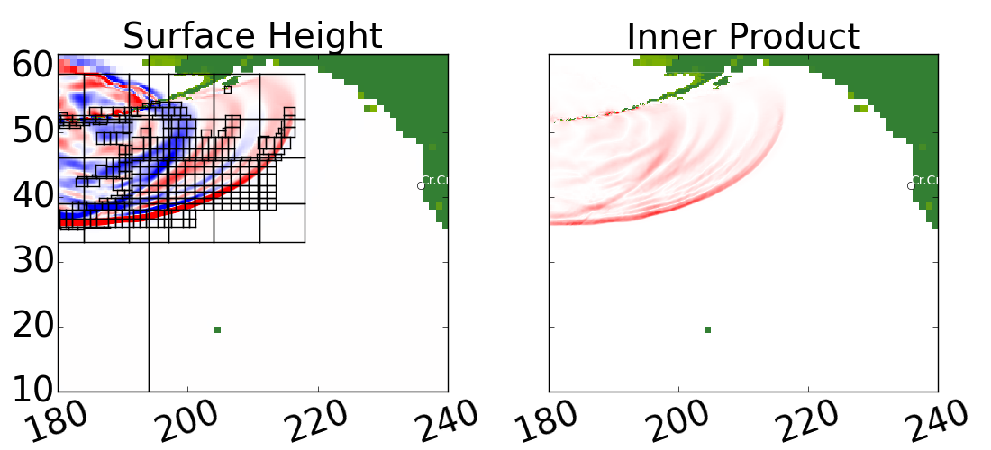
(b) Results 2 hours after the earthquake.

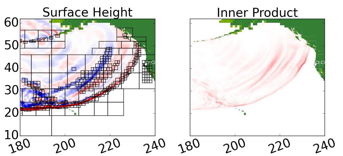
(c) Results 4 hours after the earthquake.

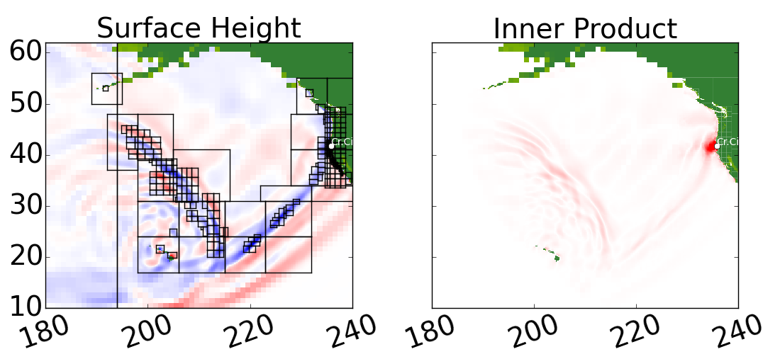
(d) Results 6 hours after the earthquake.

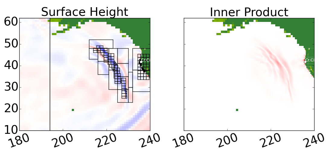
(e) Results 8 hours after the earthquake.

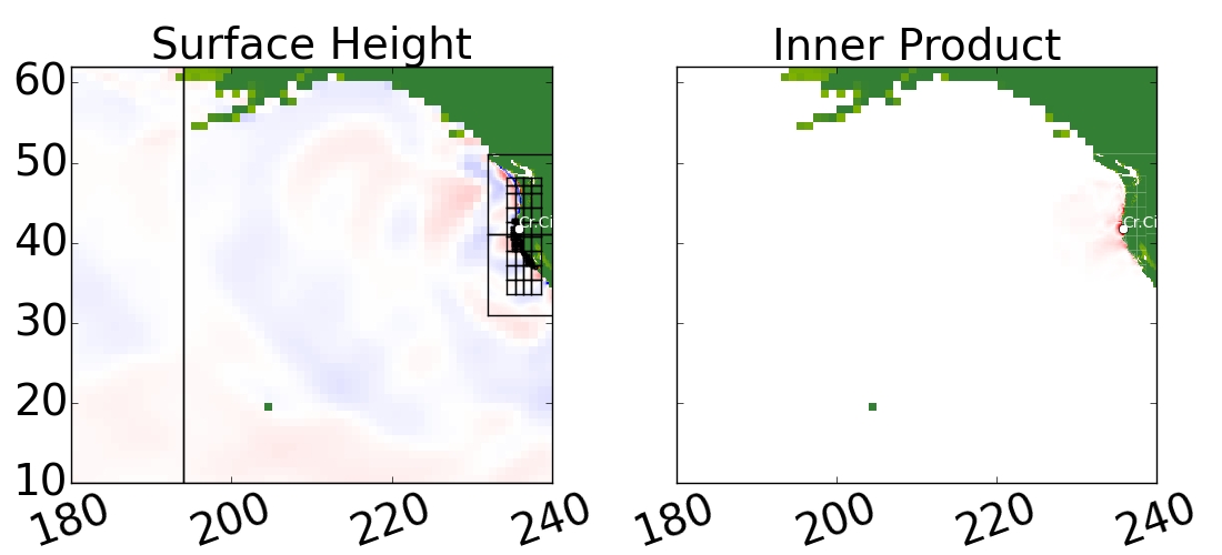
(f) Results 10 hours after the earthquake.

Figure 12: Computed results for tsunami propagation problem. The $y$-axis is the same for both plots in each subfigure. The color scale for the surface height figures goes from blue to red, and ranges between $-0.3$ and 0.3. The color scale for the inner product figures goes from white to red, and ranges between 0 and 0.05.

Fig. 12 shows the Geoclaw results for the surface height at six different times, along with the maximum inner product in the appropriate time range. Recalling that the black outlines in each figure are refined grid patch edges, it is clear that this method significantly reduced the extent of the refined regions.

5.3.1 Computational Performance

The above example was run on a quad-core laptop, for both the surface-flagging and adjoint-flagging methods, and the OpenMP option of GeoClaw was enabled which allowed all four cores to be utilized. The timing results for the tsunami simulations are shown in Table 2. Recall that two simulations were run using surface-flagging, one with a tolerance of $0.14$ (“Large Tolerance” in the table) and another with a tolerance of $0.09$ (“Small Tolerance” in the table). Finally, a GeoClaw example using adjoint-flagging was run with a tolerance of $0.004$ (“Forward” in the table), which of course required a simulation of the adjoint problem the timing for which is also shown in the table.

Table 2: Timing comparison for the example in Section 5.3 given in seconds.

Surface-Flagging		Adjoint-Flagging
Small Tolerance	Large Tolerance	Forward	Adjoint
8310.285	5724.461	5984.48	26.901

As expected, between the two GeoClaw simulations which utilized surface-flagging the one with the larger tolerance took significantly less time. Note that although solving the problem using adjoint-flagging did require two different simulations, the adjoint problem and the forward problem, the computational time required falls between the timing required for the two simulations which utilized surface-flagging.

Another consideration when comparing the adjoint-flagging method with the surface-flagging method already in place in GeoClaw is the accuracy of the results. To test this, gauges were placed in the example and the output at the gauges compared across the two different methods.

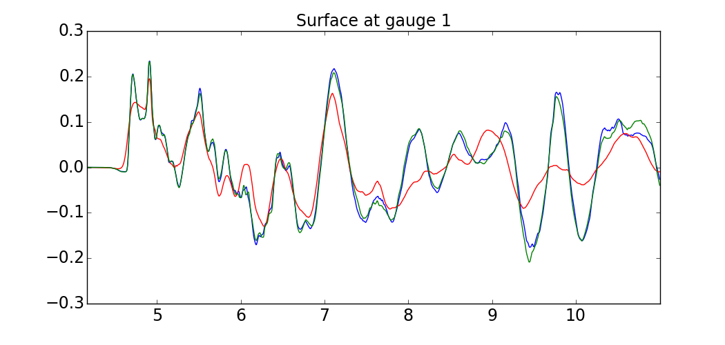
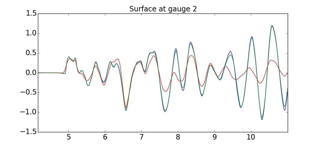
Figure 13: Computed results at gauges for tsunami propagation problem. The results from the simulation using the adjoint method are shown in blue, the results from the simulation using the surface-flagging method with a tolerance of $0.14$ are shown in red, and the results from the simulation using the surface-flagging method with a tolerance of $0.09$ are shown in green. Along the $x$-axis, the time since the occurrence of the earthquake is shown in hours.

For the tsunami example two gauges are used: gauge 1 is placed at $(x,y)=(235.536,41.67)$ which is on the continental shelf to the west of Crescent City, and gauge 2 is placed at $(x,y)=(235.80917,41.74111)$ which is in the harbor of Crescent City. In Fig. 13 the gauge results from the adjoint method are shown in blue, the results from the surface-flagging technique with a tolerance of $0.14$ are shown in red, and the results from the surface-flagging technique with a tolerance of $0.09$ are shown in green. Note that the blue and green lines are in fairly good agreement, indicating that the use of the adjoint method did not have a significant detrimental impact on the accuracy of the calculated results when compared with the smaller tolerance run using the surface-flagging method. However, the larger tolerance run using the surface-flagging method agrees fairly well only for the first wave but then rapidly loses accuracy.

6 Conclusions

Integrating an adjoint method approach to cell flagging into the already existing AMR algorithm in Clawpack results in significant time savings for all of the simulations shown here. For all three two-dimensional acoustics examples examined here, there was no visible loss of accuracy when using the adjoint method. Furthermore, the pressure-flagging technique required roughly twice as much computational time as the adjoint-flagging technique for each of the examples. It should be noted that these were rather simplified examples chosen for the sake of highlighting different aspects of the adjoint technique. With more complex examples the time savings are likely to be even larger.

For the tsunami example, the surface-flagging technique simulation with a tolerance of $0.14$ has the advantage of a low computational time but only provides accurate results for the first wave to reach Crescent City. The surface-flagging technique simulation with a tolerance of $0.09$ refines more waves and therefore provides accurate results for a longer period of time. However, it has the disadvantage of having a long computational time requirement. The use of the adjoint method allows us to retain accurate results while also reducing the computational time required.

Therefore, using the adjoint method to guide adaptive mesh refinement can reduce the computational expense of solving a system of equations while retaining the accuracy of the results by enabling targeted refinement of the regions of the domain that will influence a specific area of interest.

The code for all the examples presented in this work is available online at [15], and includes the code for solving the adjoint Riemann problems. This code can be easily modified to solve different problems. Note that it requires the addition of a new Riemann solver for the adjoint problem.

7 Future Work

The method described in this paper flags cells for refinement wherever the norm of the relevant inner product between the forward and adjoint solutions is above some tolerance. Choosing a sufficiently small tolerance will trigger refinement of all regions where the forward solution might need to be refined, and in our current approach these will be refined to the finest level specified in the computation. To optimize efficiency, it would be desirable to have error bounds based on the adjoint solution that could be used to refine the grid more selectively to achieve some target error tolerance for the final quantity of interest. We believe this can be accomplished using the Richardson extrapolation error estimator that is built into AMRClaw to estimate the point-wise error in the forward solution and then using the adjoint solution to estimate its effect on the final quantity of interest. This is currently under investigation and we hope to develop a robust strategy that can be applied to a wide variety of problems for general inclusion into Clawpack. We will also be expanding the repository of examples available online.

In this paper the adjoint solution for both the acoustics and tsunami examples was computed on a fixed grid. Allowing AMR to take place when solving the adjoint equation should increase the accuracy of the results, since it would enable a more accurate evaluation of the inner product between the forward and adjoint solutions. In an effort to guide the AMR of the adjoint problem in a similar manner to the method used for the forward problem, the two problems would need to be solved somewhat in conjunction and the inner product between the two considered for both the flagging of the cells in the adjoint problem as well as the flagging of cells in the forward problem. One approach that is used to tackle this issue is checkpointing schemes, where the forward problem is solved and the solution at a small number of time steps is stored for use when solving the adjoint problem [35]. The automation of this process is another area of future work, and involves developing an evaluation technique for determining the number of checkpoints to save or when to shift from refining the adjoint solution to refining the forward solution and vice versa.

For the tsunami example we linearized the shallow water equations about a flat surface, which we used to solve the adjoint problem. This is sufficient for many important applications, in particular for tsunami applications where the goal is to track waves in the ocean where the linearized equtions are very accurate. If an adjoint method is desired in the inundation zone, or for other nonlinear hyperbolic equations, then the adjoint equation is derived by linearizing about a particular forward solution. This would again require the development of an automated process to shift between solving the forward problem, linearizing about that forward problem, and solving the corresponding adjoint problem. Finally, in this work we assumed wall boundary conditions when a wave interacted with the coastline in the adjoint problem. This assumption, along with the use of the linearized shallow water equations, becomes significant when a wave approaches a shore line. Allowing for more accurate iterations between waves and the coastline in the solution of the adjoint problem is another area for future work.

References

- [1] V. Akcelik, G. Biros, and O. Ghattas, Parallel multiscale Gauss-Newton-Krylov methods for inverse wave propagation, in Proceedings of the 2002 ACM/IEEE Conference on Supercomputing, SC ’02, 2002, pp. 1–15.
- [2] L. Asner, S. Tavener, and D. Kay, Adjoint-based a posteriori error estimation for coupled time-dependent systems, SIAM J. Sci. Comput., 34 (2012), p. A2394–A2419.
- [3] D. S. Bale, R. J. LeVeque, S. Mitran, and J. A. Rossmanith, A wave propagation method for conservation laws and balance laws with spatially varying flux functions, SIAM J. Sci. Comput., 24 (2002), pp. 955–978.
- [4] R. Becker and R. Rannacher, An optimal control approach to a posteriori error estimation in finite element methods, Acta Numerica, 10 (2001), pp. 1–102.
- [5] M. Berger and I. Rigoutsos, An algorithm for point clustering and grid generation, IEEE T. Syst. Man Cyb., 21 (1991), pp. 1278–1286.
- [6] M. J. Berger and P. Colella, Local adaptive mesh refinement for shock hydrodynamics, J. Comput. Phys., 82 (1989), pp. 64–84.
- [7] M. J. Berger, D. L. George, R. J. LeVeque, and K. T. Mandli, The GeoClaw software for depth-averaged flows with adaptive refinement, Adv. Water Res., 34 (2011), pp. 1195–1206, www.clawpack.org/links/papers/awr11.
- [8] M. J. Berger and R. J. LeVeque, Adaptive mesh refinement using wave-propagation algorithms for hyperbolic systems, SIAM J. Numer. Anal., 35 (1998), pp. 2298–2316.
- [9] M. J. Berger and J. Oliger, Adaptive mesh refinement for hyperbolic partial differential equations, J. Comput. Phys., 53 (1984), pp. 484–512.
- [10] S. Blaise, A. St-Cyr, D. Mavriplis, and B. Lockwood, Discontinuous Galerkin unsteady discrete adjoint method for real-time efficient tsunami simulations, J. Comput. Phys., 232 (2013).
- [11] G. Buffoni and E. Cupini, The adjoint advection-diffusion equation in stationary and time dependent problems: a reciprocity relation, Rivista di Matematica della Universita di Parma, 4 (2001), pp. 9–19.
- [12] H.-P. Bunge, C. R. Hagelberg, and B. J. Travis, Mantle circulation models with variational data assimilation: inferring past mantle flow and structure from plate motion histories and seismic tomography, Geophys. J. Int., 152 (2003), pp. 280–301.
- [13] V. Carey, D. Estep, A. Johansson, M. Larson, and S. Tavener, Blockwise adaptivity for time dependent problems based on coarse scale adjoint solutions, SIAM J. Sci. Comput., 32 (2010), pp. 2121–2145.
- [14] Clawpack Development Team, Clawpack software, 2015, http://www.clawpack.org. Version 5.3.
- [15] B. N. Davis, Adjoint code repository, https://github.com/BrisaDavis/adjoint.
- [16] D. L. George, Augmented Riemann solvers for the shallow water equations over variable topography with steady states and inundation, J. Comput. Phys., 227 (2008), pp. 3089–3113.
- [17] M. B. Giles and N. A. Pierce, An introduction to the adjoint approach to design, Flow Turbul. Combust., 65 (2000), pp. 393–415.
- [18] M. C. G. Hall, Application of adjoint sensitivity theory to an atmospheric general circulation model, J. Atmos. Sci., 43 (1986), pp. 2644–2652.
- [19] A. Jameson, Aerodynamic design via control theory, J. Sci. Comput., 3 (1988), pp. 233–260.
- [20] G. J. Kennedy and J. R. R. A. Martins, An adjoint-based derivative evaluation method for time-dependent aeroelastic optimization of flexible aircraft, in Proceedings of the 54th AIAA/ASME/ASCE/AHS/ASC Structures, Structural Dynamics, and Materials Conference, Boston, MA, April 2013. AIAA-2013-1530.
- [21] R. J. LeVeque, Wave propagation algorithms for multidimensional hyperbolic systems, J. Comput. Phys., 131 (1997), pp. 327–353.
- [22] , Finite Volume Methods for Hyperbolic Problems, Cambridge University Press, 2004.
- [23] R. J. LeVeque, D. L. George, and M. J. Berger, Tsunami modeling with adaptively refined finite volume methods, Acta Numerica, (2011), pp. 211–289.
- [24] S. Lia and L. Petzold, Adjoint sensitivity analysis for time-dependent partial differential equations with adaptive mesh refinement, J. Comput. Phys., 198 (2004), pp. 310–325.
- [25] K. T. Mandli and C. N. Dawson, Adaptive mesh refinement for storm surge, Ocean Modelling, 75 (2014), pp. 36–50, doi:10.1016/j.ocemod.2014.01.002, http://www.sciencedirect.com/science/article/pii/S1463500314000031 (accessed 2015-04-28).
- [26] J. Marburger, Adjoint-based optimal control of time-dependent free boundary problems, 2012, http://arxiv.org/abs/1212.3789.
- [27] A. Mishra, K. Mani, D. Mavriplis, and J. Sitaraman, Time-dependent adjoint-based optimization for coupled aeroelastic problems, in 31st AIAA Applied Aerodynamic Conference, San Diego, CA, 2013. AIAA 2013-2906.
- [28] M. Nemec and M. J. Aftosmis, Adjoint error estimation and adaptive refinement for embedded-boundary Cartesian meshes, in 18th AIAA Computational Fluid Dynamics Conference, 2007.
- [29] M. Nemec, M. J. Aftosmis, and M. Wintzer, Adjoint-based adaptive mesh refinement for complex geometries, 46th AIAA Aerospace Sciences Meeting, (2008).
- [30] C. Othmer, Adjoint methods for car aerodynamics, Journal of Mathematics in Industry, 4 (2014), 6.
- [31] B. F. Sanders and S. F. Bradford, High-resolution, monotone solution of the adjoint shallow-water equations, Int. J. Numer. Meth. Fluids, 32 (2002), p. 139–161.
- [32] B. F. Sanders and N. D. Katopodes, Adjoint sensitivity analysis for shallow-water wave control, J. Eng. Mech., 126 (2000), p. 909–919.
- [33] J. Tromp, C. Tape, and Q. Liu, Seismic tomography, adjoint methods, time reversal and banana-doughnut kernels, Geophys. J. Int., 160 (2005), pp. 195–216.
- [34] D. A. Venditti and D. L. Darmofal, Adjoint error estimation and grid adaptation for functional outputs: Application to quasi-one-dimensional flow, J. Comput. Phys., 164 (2000), pp. 204–227.
- [35] Q. Wang, P. Moin, and G. Iaccarino, Minimal repetition dynamic checkpointing algorithm for unsteady adjoint calculation, SIAM J. Sci. Comput., 31 (2009), pp. 2549–2567.