Bayesian parameter estimation for effective field theories
Abstract
We present procedures based on Bayesian statistics for estimating, from data, the parameters of effective field theories (EFTs). The extraction of low-energy constants (LECs) is guided by theoretical expectations in a quantifiable way through the specification of Bayesian priors. A prior for natural-sized LECs reduces the possibility of overfitting, and leads to a consistent accounting of different sources of uncertainty. A set of diagnostic tools are developed that analyze the fit and ensure that the priors do not bias the EFT parameter estimation. The procedures are illustrated using representative model problems, including the extraction of LECs for the nucleon mass expansion in SU(2) chiral perturbation theory from synthetic lattice data.
pacs:
02.50.-r, 11.10.Ef, 21.45.-v, 21.60.-nI Introduction
Effective field theories (EFTs) describe physics in the presence of a separation of scales. They exploit known symmetries to construct general interactions at the lower momentum scale that do not depend on unresolved details of the physics from the higher scale Kaplan (1995); Phillips (2002); Burgess (2007); Epelbaum (2010). A ratio (or, in the case of multiple scales, ratios) between the separated scales is formed, enabling a power-counting scheme that organizes the (renormalized) contributions of different operators to observables in an order-by-order expansion in the ratio(s) Epelbaum (2010). The effects of unresolved physics are parametrized by the coefficients of these operators, called low-energy constants (LECs). Estimating these LECs using experimental data or numerical simulations of the underlying theory is essential if the EFT is to be used to make quantitative predictions. But, since the EFT expansion is written in terms of a ratio of disparate scales, even in the absence of such data, we expect the LECs in the EFT should be of “natural” size, that is, of order unity when expressed using the appropriate scales.
In this paper we lay out a framework for EFT practitioners to obtain estimates of the LECs in their EFT while incorporating all the information at their disposal. A Bayesian formulation of the problem is ideal for this, as it facilitates folding theoretical expectations—such as that the LECs should be natural—into parameter estimation. Using only data (together with their statistical errors) to constrain the LECs can lead to distortions in the fits; this is already recognized by EFT practitioners who adapt their fitting procedures to include additional information (e.g., in fitting NN scattering data, see Sec. II.1). The use of priors is thus very well motivated in the EFT context. Even though it is still controversial in other contexts, such Bayesian reasoning has recently found several significant applications in EFTs for nuclear physics Descotes-Genon et al. (2004); Ledwig et al. (2014); Zhang et al. (2015); Furnstahl et al. (2015a); Pérez and Papenbrock (2015); Griesshammer et al. (2015). But priors can bias the parameter extraction if not used carefully. Validating the prior is a key element of robust parameter estimation.
The naturalness priors and Bayesian framework also allow us to examine the impact of higher-order terms in the EFT. Those terms can be incorporated into the fit, either through a known functional form or via the assumed EFT expansion for observables (see Ref. Furnstahl et al. (2015a)), and then accounted for using the rule of marginalization. This allows the parameter estimation to account for all three sources of uncertainty in the extraction of LECs Furnstahl et al. (2015b):
-
1.
Data uncertainties from experiment or numerical simulations.
-
2.
Systematic errors from truncating the EFT.
-
3.
Errors from methods used to compute observables.
These uncertainties are often intertwined and must be dealt with consistently, and each is nontrivial to estimate. For example, even when there is a large amount of high-quality data available, as in the case of NN scattering, that data must be carefully analyzed for consistency, as in the self-consistent database of Ref. Navarro Pérez et al. (2013). But, while errors of the first type are often included in LEC extractions—and errors of the third type are sometimes also accounted for—it is far rarer for such extractions to consider the systematic errors from truncation of the EFT. Yet neglecting those means we fail to incorporate all the information we have about the EFT when determining the best values for LECs.
Using information on LEC naturalness also ameliorates the well-known phenomena of “overfitting” and “underfitting” within the EFT:
-
Overfitting. The parameters get fine-tuned to the data. A naturalness prior reduces the risk of this, since it restricts degenerate directions in the EFT parameter space. Together with marginalization over higher orders, the prior additionally ensures that the LECs are not tuned to reproduce the data better than expected from the theoretical truncation error.
-
Underfitting. The model provides an inadequate representation of at least part of the data being fit (e.g., not high enough order). Marginalization over higher EFT orders ensures that the combined data and truncation uncertainties—which together determine the total uncertainty of the LECs—grows as the EFT parameter increases. Without this feature, blind application of least-squares fitting can lead to low-order LECs being overly influenced by data in an energy domain where the corresponding EFT expression has large errors.
When conducting EFT parameter estimation using data over a large range of the expansion parameter, it is possible to experience tendencies toward both overfitting and underfitting. In the past these biases have usually been decoupled in EFT fits by limiting the parameter range over which data are fitted. But, ideally, all available data would be used to inform results. A well-constructed prior protects against these biases while simultaneously relieving the scientist of the responsibility of justifying an arbitrarily chosen cutoff of data. We will show that our Bayesian EFT parameter estimation converges simply and intuitively, and that it does so even for data sets that include regions where the EFT converges poorly, or not at all.
This is achieved by computing so-called posterior probability distributions (pdfs) for LECs with all assumptions, such as naturalness, made explicit. We develop a system of diagnostics that ensure consistent, reproducible posteriors, with all assumptions manifested through the use of Bayesian priors. The diagnostics also allow tests of the sensitivity to particular prior prescriptions. Such a framework avoids both overfitting and underfitting in a statistically well-defined way, thereby maximizing the information from data that enters the LEC determination.
The probability distributions yield estimates of the parameters of the effective theory that are derived from both the data considered and underlying knowledge of the theory itself. Propagating the resulting uncertainties to the EFT’s predictions displays the impact that uncertainties in the data used to fix the LECs have on those predictions. By combining those results with our prescription for truncation errors from Ref. Furnstahl et al. (2015a) we can fully account for the uncertainties in the EFT (we do not address here the uncertainties from calculational methods, although their inclusion is well defined), thereby providing reliable guidance as to the power of new experimental or lattice data to improve theoretical predictions.
Following Refs. Schindler and Phillips (2009a); Furnstahl et al. (2015b), where a model problem was introduced to simulate the systematic behavior of an EFT expansion, we will explore representative examples to demonstrate issues that occur in EFT parameter estimation. To simulate the extraction of EFT parameters from data, we contrive functions of a single variable, say, . This function is designed to have a Taylor series whose coefficients are order unity within a radius of convergence that is equal, or close, to 1:
| (1) |
The s play the role of LECs in this example. They are extracted from synthetic data to which Gaussian noise is added to simulate experimental errors. In this case, the data are generated by choosing a set of —typically evenly spaced— points up to a maximum value of ; given the point , the data point and error are
| (2) |
where is normally distributed with mean 0 and standard deviation 1. is a specified relative error.
The goal of the model problems is then to reliably estimate as many EFT parameters as possible given certain synthetic data. We do this by choosing a truncation order for the “theory” (which is really just a polynomial) and determining the posterior pdfs of the coefficients in
| (3) |
from the data.111The extension to an EFT with multiple coefficients at a given order and/or more than one expansion parameter because of multiple low-energy scales follows by generalizing the vector of coefficients (e.g., see Sec. V.3). To ensure that the extraction is robust and reliable, one includes by a marginalization integral the contributions from a (hopefully finite) number of influential higher-order coefficients up to some order . This accounts for the uncertainties in the posterior that arise as an artifact of finite-order truncation of the EFT, as presented in Ref. Furnstahl et al. (2015a). For the simple models here, this marginalization is the same as doing parameter estimation up to truncation order .
These model problems allow us to control the “natural” size of the coefficients being determined, the distribution and range of the “experimental” data, and its precision. We can explore pertinent EFT issues such as the presence of unnatural coefficients or improvements gained by adding new data, while avoiding the computational cost of computing observables from EFTs order-by-order.
However, such models do not include certain generic aspects of actual EFTs. An obvious extension of Eq. (3) is to a problem with two light scales, as occurs in chiral perturbation theory (PT), where the pion mass and the (assumed small) external momentum can be used to form two independent expansion parameters. Here we deal only with series in one variable; the extension to additional variables should be straightforward.
Another aspect of EFTs which is not reflected in Eq. (3) is that the coefficient of the term of will typically be a non-analytic function of , , of which the LEC forms only the constant part. For the parameter-estimation problems being discussed here it is crucial that the non-analytic parts of —i.e. all but the LEC that appears in it—are predicted by the EFT. (Indeed, at certain orders in the EFT expansion contains no LEC and is completely predicted.) Thus, up to the order to which the EFT series has been computed, these non-analytic pieces can be removed from the parameter-estimation problem by simply subtracting them from the data. Of course, such a subtraction is only feasible for orders where the are known. But, at all orders in the EFT, the should be for in the domain where the EFT applies. This allows us to deal with higher-order terms in the EFT series by imposing a naturalness prior on unknown higher-order coefficients—even in this general case where the coefficient is, in fact, a function—thereby facilitating marginalization over the higher-order terms.
Such non-analytic terms occur in one of our examples: the estimation of LECs for the two-flavor PT expansion of nucleon mass up to sixth chiral order. In this application, which was previously considered in Ref. Schindler and Phillips (2009a), the LECs are linearly related to the data used for the extractions, just like our generic polynomial model. This example is difficult because it involves extracting a relatively large number of LECs from lattice data in a region where contributions at different orders are not easily distinguished.
In anticipation of later applications to chiral EFT for nuclei, we also examine the impact on our procedures of situations where the quantity for which we have data is a nonlinear function of the LECs . In addition, we will need to account for higher-order contributions to the posterior when they have an unknown form or are impractical to compute. Our strategy is to build upon Ref. Furnstahl et al. (2015a) and use the expected naturalness of the expansion coefficients for the fit observables rather than the LECs themselves above the order . This alternative approach is discussed in Sec. III.1.
In Sec. II, we first briefly review alternative procedures used to supplement standard least-squares methods when fitting LECs for chiral EFT, and then outline our Bayesian framework for EFT parameter estimation. Sec. III gives an overview of the procedures and diagnostics for LEC estimation, illustrated with a particular model problem. A flowchart for using the diagnostic framework is presented in Sec. IV and the major steps are illustrated with examples using a different model. Additional case studies, including a nonlinear model and the PT mass expansion, are briefly explored in Sec. V. In Sec. VI we summarize and present plans for future analyses with the diagnostic framework by the BUQEYE222Bayesian Uncertainty Quantification: Errors for Your EFT. collaboration.
II Statistical Methods
II.1 Least-squares minimization
The underlying basis for extracting LECs is generally minimization of a least-squares objective function for a set of observables (e.g., see Ekström et al. (2013)):
| (4) |
where is the value of the EFT expansion parameter at which the observable was measured, is the total number of data, is the experimental measurement of the observable, is the corresponding EFT prediction at given a set of LECs (which we denote collectively as the vector ), and is the uncertainty associated with the observable. A conventional least-squares minimization would take to be the experimental error, but, as already noted, in practice the procedure is modified to take account of additional elements, such as theoretical errors. Recent fits made of LECs for nucleon-nucleon scattering in chiral EFT in Ref. Carlsson et al. (2015) and Ref. Epelbaum et al. (2015), which apply different regularization schemes, provide representative examples of the modifications.
Carlsson et al. add the different sources of uncertainty in quadrature for each observable Carlsson et al. (2015),
| (5) |
where is the experimental uncertainty, and are computational uncertainties (both included as the third type of uncertainty listed in the Introduction), and is the systematic EFT truncation error. The latter is estimated for scattering at momentum as a constant times the expected expansion parameter raised to a power given by the first omitted order (), namely , with the breakdown scale of chiral EFT. The constant is determined self-consistently by requiring that including the full of Eq. (5) equals the number of degrees of freedom, as advocated in Ref. Dobaczewski et al. (2014).
Epelbaum et al. Epelbaum et al. (2015) use but address the danger of underfitting by limiting the region of fit data according to estimates of the domain of validity at each EFT order. They also augment the function with penalty terms to enforce an expected relation between two LECs (Wigner symmetry) and to limit the allowed range of the D-state probability of the deuteron. These serve to restrict the parameter space for the least-squares fit, which limits overfitting. As part of the uncertainty quantification (but not the fit itself), error estimates are made based on expectations for truncation errors. In Ref. Furnstahl et al. (2015a), these estimates were shown to be justified semi-quantitatively by Bayesian arguments and a naturalness prescription.
The Bayesian approach we advocate for parameter estimation has a different structure to the procedures of Ref. Carlsson et al. (2015); Epelbaum et al. (2015); it is an interesting and relevant question whether those procedures can also be derived or motivated by a Bayesian framework under prescribed conditions. For example, in Ref. Furnstahl et al. (2015b), it was noted (drawing on Stump et al. Stump et al. (2001)) that when Gaussian priors are used one can account for missing higher-order contributions by a modified, augmented . However, this does not take the form of adding experimental and theory errors in quadrature as in Eq. (5). We do not intend to pursue these connections further here. Rather we have sketched these examples to highlight that the use of a priori supplementary information is standard practice in state-of-the-art LEC optimization.
II.2 Bayesian parameter estimation
We generically use the notation to denote the pdf of given that is true. The Bayesian framework for parameter estimation determines the posterior , which is the joint probability distribution for the full set of LECs given the data (including their errors) and any other information . includes the form of the EFT expansion and the order at which it is truncated, together with additional knowledge such as the expected naturalness of the LECs. We emphasize that the posterior distribution contains much greater content than just the “best-fit” values for the coefficients (which might, but need not necessarily, be identified as the vector that maximizes the posterior). When a Gaussian approximation to the posterior is appropriate, the full content may be effectively summarized by values for the maximum and a covariance matrix. But, for determining how the uncertainties propagate, it is generally necessary to start with the full posterior.
To make progress, we express the desired pdf in terms of other pdfs that we can calculate or use to implement prior information, e.g., about naturalness. This is done using the basic rules of probabilistic inference, the sum and product rules, and their immediate consequences such as Bayes’ theorem and marginalization Gregory (2005); Sivia and Skilling (2006). It was demonstrated by Cox that this is the unique set of rules that follow from basic postulates of consistency Cox (1946, 1961); Jaynes (2003).
The product rule dictates two ways to decompose a joint probability:
| (6) |
A simple rearrangement of the two decompositions yields Bayes’ theorem, which when applied to the posterior for parameter estimation yields
| (7) |
The pdf in the denominator, , which is called the evidence for , has no dependence on and is therefore determined here by normalization. (In this context the normalization follows from the sum rule for probabilities, but the unnormalized magnitude of the resulting integral is useful in Bayesian model selection, see Sec. II.5 below.) Rewriting Eq. (7) as a proportionality, we have
| (8) |
The posterior is therefore determined by the product of two probabilities, the likelihood and the prior . The Bayesian procedure for estimating LECs proceeds by identifying a likelihood based on the available experimental data, assigning an appropriate prior, and finally analyzing the properties of the posterior for , including the dependence on the choice of prior. From the computed posterior, we can propagate the LEC uncertainties to the predictions of the EFT. We describe the practical implementation of this procedure in Sec. III. We pay particular attention to problems that can occur if the prior is not well chosen and develop a set of diagnostics by which such problems may be identified.
The unadorned least-squares minimization procedure with follows from particular choices for the likelihood and prior. The pdf for independent data given the LECs and relevant information including the form and truncation order of the EFT is given by
| (9) |
with the objective function defined in Eq. (4).333The principle of maximum entropy (MaxEnt) Jaynes (1957) can be used to derive this likelihood in the Bayesian framework Gregory (2005); Sivia and Skilling (2006). In general we need a covariance matrix to account for correlated data. Note that the theory itself, including the LECs and all other pertinent information, is on the right-hand side of the conditional here, i.e., it is given information. If we identify the “best-fit” parameters with the maximum of the posterior from Eq. (8) (maximum likelihood), then the Bayesian procedure is equivalent to least-squares minimization if we choose the prior to be uniform (i.e., independent of ) in regions where the likelihood is nonzero (or non-negligible). This equivalence does, though, blur the significant interpretative difference between and . This difference in frequentist and Bayesian perspectives will be discussed in Sec. II.4
One might think that a uniform prior is a natural, unbiased choice, but there are subtleties (e.g., in what variable it should be uniform and whether uniformity accounts for all available constraints) Sivia and Skilling (2006). Furthermore, in the context of EFTs we know that the LECs should not have any unrestricted value, but instead can be expected to be distributed in some “natural” range around zero. Thus a uniform prior encodes information that is not expected, namely that parameters in any interval are equally likely. But this prior is the baseline for many analyses, and so we use it throughout as a benchmark. We will use the term “least-squares fit” interchangeably with maximizing the posterior of using a uniform prior. However, we stress again that in practice, especially in the EFT context, least-squares is often augmented with other criteria, such as those reviewed in Sec. II.1.
II.3 Marginalization
The sum rule of probabilities says a pdf should be normalized, that is,
| (10) |
where the integration is over the appropriate range of . The sum rule implies that for a joint pdf we find
| (11) |
which is marginalization, with the product rule applied to obtain the second form.
This rule allows us to “integrate out” parameters from a joint distribution to obtain a pdf which depends only on the parameter(s) of interest. One can also “integrate in” parameters, expressing a pdf for some parameters in terms of integrals over joint distributions with other parameters. This is especially useful when the form of a pdf of interest is not known, but joint distributions with other parameters are known.
We use the rule of marginalization extensively in several different contexts.
-
1.
Projection: to quote LEC results and plot pdfs. We derive two-dimensional pdfs from the full joint posterior by integrating over all the other parameters:
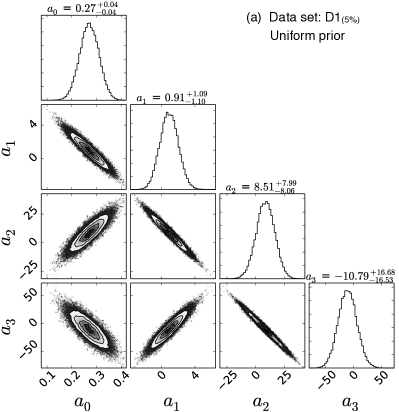
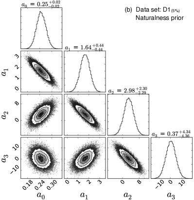
(12) Such marginalized posteriors for the model used in Refs. Schindler and Phillips (2009a); Furnstahl et al. (2015b) are shown in the plots below the diagonal in Fig. 1, where the -axis scale is at the bottom. (This model will be used in Sec. III to illustrate the general procedures and diagnostics.) The s are displayed as intensity plots, and so reveal the regions of high joint probability for pairs of LECs. Such projected posterior plots are therefore useful for diagnosing correlations between the LECs obtained from the analysis. Further details of their interpretation will be discussed in Sec. III.2. Note that in this case, the posteriors are two-dimensional Gaussians, but in general they can be more complicated and even multi-modal.
One further marginalization step reduces the two-dimensional pdfs to one-dimensional pdfs for a particular LEC, i.e.
(13) These pdfs appear on the diagonal in Fig. 1. Here, the individual posteriors are simple Gaussians, but again, in general, they can be highly non-Gaussian.
-
2.
Higher orders: to account for higher-order terms in the EFT expansion and avoid underfitting when extracting low-order LECs. Marginalization is a straightforward method to account for such higher-order terms whose coefficients may not be well-constrained by the data but can still be assumed to be natural. In particular, if we need to determine coefficients up to order but wish to account for contributions up to order , we marginalize according to
(14) -
3.
Integrating in: to describe pdfs of interest in terms of pdfs with known analytic forms. For example, the prior distribution can be expressed in terms of a naturalness parameter,
(15) where parameterizes the width of prior pdf for the LECs . By introducing the marginalization integral over , the prior for the LECs is specified quantitatively by its width and can be calculated.
II.4 Interpretation
In Sec. II.2 we noted how the Bayesian procedure can yield the same maximum likelihood result obtained from a frequentist procedure. However, the interpretations are quite different. In the strict frequentist view, the only valid interpretation of probability is as the relative frequency of an event out of a large ensemble of repeatable experiments Olive et al. (2014). Thus the outcomes of experiments are treated as random variables. Model parameters (e.g., the LECs), on the other hand, are fixed — they do not have a probability distribution, so the Bayesian posterior we seek has no meaning. The complete focus is on the likelihood. Thus, strictly speaking, a frequentist confidence interval (CI) exists only for data. It gives the probability that, for fixed parameters, a large set of experiments will yield results that fall in the interval % of the time.
In the Bayesian interpretation, probabilities express the current state of knowledge about the parameters, which allows us to calculate Bayesian degree-of-belief (DoB) intervals for the true values of the parameters. These are established by integrations over posteriors for (or some subset) to determine the desired intervals. For example, a 68% DoB interval for a parameter means that the particular input data and information lead to a probability of 68% that the true value of is in that interval. The data are fixed while the parameters have a pdf.
The use of the word “belief” here is somewhat unfortunate, because it might suggest to some readers that results are subjective. And indeed, different priors can lead to different outcomes for the posterior pdfs—particularly in the case where data are sparse or of low quality. But, the Bayesian framework is completely rigorous once the prior is specified. It permits a careful tracing of assumptions through to probabilistic consequences for parameters. In the case of EFT the assignment and interpretation of the prior should not be a source of controversy: it merely encodes a priori information about the parameter of interest. Furthermore, the prior can also represent knowledge from previous determinations or measurements. The use of Bayesian priors thus provides a quantifiable way to include guidance from both theory and previous experiments. It makes explicit the assumptions that are inherent in EFT parameter estimation, but are usually left largely implicit. We also mention in this context that, given specified pieces of “testable information” for the parameters, the Method of Maximum Entropy (MaxEnt) Jaynes (1957) can be used to derive the least informative priors based on the known information.
The interplay of likelihood and prior in limiting cases embodies desired outcomes that otherwise have to be imposed by hand. If the data are numerous and of good quality, a highly peaked likelihood will be the dominant contribution to the posterior if the prior is not too restrictive Sivia and Skilling (2006). On the other hand, if the likelihood for a parameter is not well-constrained by the data, the prior will have the dominant effect. In the case of LEC parameter estimates, a naturalness prior can restrict the effect of parameters that are not well-constrained by data by suppressing contributions from regions of parameter space driven by spurious correlations.
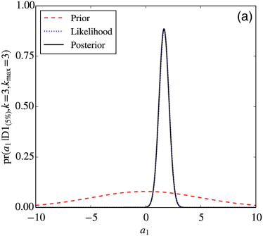
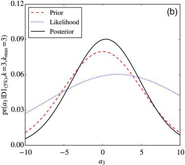
An example of a parameter that is well-determined by data is shown in Fig. LABEL:sub@fig:likelihood-win, where the prior does not affect the posterior for that parameter because it is essentially uniform in the region where the likelihood has support. Figure LABEL:sub@fig:prior-win shows an example where the posterior largely reflects the input prior, since the parameter is not strongly localized by the slowly varying likelihood. We refer to this latter situation as the posterior “returning the prior”. These are marginalized posterior distributions from the same joint pdf , which means that even though the prior does not seem to play a role in Fig. LABEL:sub@fig:likelihood-win, this is because it has restricted the domain of the parameter in Fig. LABEL:sub@fig:prior-win. Thus the first parameter is insensitive, but only because the prior prevented other, higher-order, parameters from contributing in unnatural regions of parameter space. An example of a spurious correlation can be seen in Fig. LABEL:sub@fig:triangle_D1_uniform, where is correlated with the ill-determined cubic coefficient . The amelioration of this problem is then seen in Fig. 1LABEL:sub@fig:triangle_D1_Gaussian, where the correlation is almost completely removed when an appropriate naturalness prior is applied.
II.5 Bayes evidence
In this section we explain how Bayesian methods facilitate a quantitative approach to model selection: which model from a set of models is preferred by the data? Our presentation draws on material from Refs. Sivia and Skilling (2006); Gregory (2005); Trotta (2008).
We should first clarify what we mean by “model” in this context. After all, an EFT is said to be model-independent because the theory is constructed in the most general form consistent with the symmetries of the underlying interaction. We use “model” here to mean any theoretical construct for computing an observable. Examples of quantitative Bayesian comparisons between EFT models could be the predictive power of EFTs with different degrees of freedom for the same data set, or an analysis of the increase in predictive power for observables using different orders in the same EFT.
For two models and and the same data set , the relevant pdfs to compare are the posteriors for each model given the data, called the model evidence: and . Note that there is no reference to a particular parameter set here; the comparison is not between two fits but between two models. We can use Bayes’ theorem to express the evidence ratio for the two models:
| (16) |
where the common factor of cancels in the ratio. If neither model is a priori more likely, the ratio so that the evidence ratio becomes equal to the Bayes factor
| (17) |
To express the right-hand-side in terms of the parameters of each model, we apply the marginalization rule so that
| (18) |
Thus we integrate over the entire parameter space. The evidence ratio provides a quantitative diagnostic to assess the effectiveness of EFTs with different degrees of freedom (e.g., comparing EFT with and without explicit -resonances Epelbaum et al. (2008)) or distinguishing between different power-counting schemes.
Here we focus on using the evidence ratio to assess whether adding another order to our EFT is favored by the given data. Thus we consider the case where and are the same EFT but evaluated at successive orders in the EFT expansion, and that neither is more likely a priori so that the evidence ratio for the two models is equal to the Bayes factor as in Eq. (17). (We will continue to use and to denote the corresponding vectors of coefficients.)
For simplicity, let have one additional parameter and assume that the priors for the parameters factor into individual priors, so
| (19) |
If the values of that contribute to the integrand in the numerator of Eq. (18) are determined predominantly by the likelihood (for the values of where the integrand is large), and that likelihood is sharply peaked, then we can approximate the impact of the prior by taking it to be roughly constant with an effective width , so . We then approximate the integral over as the value at the likelihood peak times the width of that peak, . This yields the Bayes factor
| (20) |
The ratio of integrals represents the gain in the likelihood from having this extra parameter with value . But the ratio is also multiplied by the “Occam factor” or “Occam penalty” , which is the factor by which the parameter space collapses when the data are taken into account (this is large when the parameters can range over a large domain compared to the restriction imposed by the data).
Equation (20) tells us that we will favor the more complicated model only if the likelihood gain is larger than this factor. We are assuming that is contained within , i.e., is with , which means this likelihood gain is always greater than or equal to one. In a situation such as Fig. LABEL:sub@fig:likelihood-win, we have a peaked likelihood compared to the prior pdf, which yields a substantial Occam penalty. However, the likelihood gain here is much greater than that penalty, because it involves the likelihood peak at in comparison to the likelihood for , and the latter is very small. That means that the evidence ratio for the addition of is , and the inclusion of this parameter is therefore highly favored. This leads us to expect that if we calculate the evidence for the data as a function of the order (which we will henceforth call the “evidence” for brevity) that function will increase as long as additional parameters are leading to a marked decrease in the . However, if the likelihood function at is not well below the peak value (e.g., its width is greater than in this example, or the peak is shifted toward zero), than the Occam penalty can dominate and disfavor an additional parameter, which is an implementation of Occam’s razor. In such a situation the evidence will decrease from order to order . We would then expect the evidence function to show a peak.
A different behavior can be expected if the comparison of likelihood and prior as in Fig. LABEL:sub@fig:prior-win holds, in which case the analysis of Eq. (18) is inverted. That is, we now say that the dependence on in the likelihood can be replaced by a constant and the likelihood pulled out of the integral of :
| (21) |
The integral over is now just a normalization integral, equal to one. We are dominated by the prior, so and the Bayes ratio is one, because with the last coefficient equal to zero is simply . The same argument goes through for each higher value of , meaning that we have saturation rather than a peak for as a function of the order Trotta (2008). In summary, the naturalness prior cuts down the “wasted” parameter space that might be ruled out by the data and which leads to an Occam penalty. This means that it limits the “phase space” of an EFT, which is therefore a simpler model (in the model selection sense) than the same functional form with unconstrained or only weakly constrained LECs.
II.6 Sampling with MCMC
While in some situations it is possible to evaluate posterior pdfs analytically, in many cases we must resort to numerical methods. Although many of the integrals we confront in this present work do not require its use, we employ Markov Chain Monte Carlo (MCMC) sampling methods to obtain posterior pdfs, since they are easily generalized to cases with more complicated probability distributions.
The MCMC algorithm generates samples according to the posterior probability distribution . Expectation integrals may then be performed using those samples:
| (22) |
The result accounts for all correlations between the parameters. The propagation of those correlations to the function can be simplified if the posterior is well approximated as a correlated Gaussian; in that case the correlation matrix can be employed for this purpose. But Eq. (22) achieves this task independent of whether is Gaussian or not. Marginalization integrals over parameters [see, e.g., Eq. (12)] can also be performed trivially by retaining only samples in the parameters of interest. The samples are constructed via MCMC, in a particular implementation called emcee Foreman-Mackey et al. (2013). Implementation details can be found in Appendix A.
III Diagnostics and procedures for parameter estimation
III.1 Set up of a test case
In this section we present a suite of diagnostics and associated procedures for EFT parameter estimation. For continuity, we use for illustration a model problem explored in previous work Schindler and Phillips (2009a); Furnstahl et al. (2015b), which is to use a given data set to extract as many coefficients in a particular function’s Taylor expansion as possible. For the function we choose, in this section Schindler and Phillips (2009a):
| (23) |
The function is designed to have coefficients that are up to about tenth order, and the singularity at means this is where the simulated EFT expansion breaks down. We follow the previous work and consider 10 equally spaced data points covering the range , each with a data error of 5% [thus in Eq. (2)]. The data set is enumerated in Appendix C of Ref. Schindler and Phillips (2009a) and is also available as supplementary material to this paper. To conform to later usage, we refer to this as data set , where “D” indicates the function defined by Eq. (23), the “1” labels a choice of points where the function was sampled, and the subscript indicates the data error. Other models and the nucleon mass expansion, with varied data ranges, precision, and numbers of points, will be considered in Secs. IV and V.
| set | ||
|---|---|---|
| A | ||
| A′ | ||
| B | ||
| C | ||
| C′ |
| Name | Fig. | Description and uses |
|---|---|---|
| projected posterior plot | 1 | Matrix of subplots with posteriors from marginalizing over all but one (diagonal) or all but a pair (lower triangle). Compare different priors; visualize correlations; identify when posterior prior. |
| posterior | 6 | . Show weighting of values when marginalized; identify appropriate marginalization range for ; signals unnatural coefficients. |
| relaxation plot | 7 | Evolution of marginalized posterior for single coefficients for full range of . Check whether is too restrictive (rapid changes with ); identify regions insensitive to to help identify marginalization range; show transition to least-squares result. |
| evidence vs. | 8 | (if uniform prior on ). Show transition from dominance by likelihood [e.g., Fig. LABEL:sub@fig:likelihood-win] to dominance by prior [e.g., Fig. LABEL:sub@fig:prior-win]. |
| plot | 9 | Evolution of marginalized posterior for single coefficients, , as data range specified by is increased. Check for stability with data range. |
| multi-set plot | LABEL:sub@fig:D15_datasets | Evolution of marginalized posterior for single coefficients using multiple equal-sized sets of data, each over the same range. |
| accumulation plot | LABEL:sub@fig:D15_accumulated | Comparison of marginalized posteriors for single coefficients as data are accumulated from combining multiple equal-sized sets of data. |
| residual plot | 12 | Log-log plot of residuals versus expansion parameter . Check for power-law behavior at different orders. Test for data or theory error dominance in different regions of . |
Now that we have data for a simulated EFT, the first step in our analysis is to select prior pdfs for the coefficients. Some possible sets of priors encoding naturalness assumptions are listed in Table 1. Prior Sets A, B, and C were used in Ref. Furnstahl et al. (2015a). The assumption for the coefficients themselves (the s) in Sets A and B correspond to a flat distribution bounded by a maximum, . For Set A, this naturalness parameter is itself subject to a scale-invariant uniform (Jeffreys) prior Schindler and Phillips (2009a) between the limits and , while Set B has the naturalness parameter following a log-normal distribution of width . Set C assumes a Gaussian prior distribution for the s, with the width distributed according to the Jeffreys prior. In general, arguments can be made to support any of these assumptions, which means we need to carefully check the sensitivity of our results to different choices.
For most of our examples, we choose a simpler variation of Set C, labeled Set C′, in which we adopt the Gaussian prior on the coefficients ,
| (24) |
where will include the order of the model and the marginalization order, and fix the value of the naturalness parameter at :
| (25) |
so that the marginalization over as in Eq. (15) picks out this value. The impact of the choice of a particular can be anticipated by consulting the posterior plot described below.
We seek the posterior for the parameters for the model EFT expansion up to order , but we will marginalize over coefficients as in Sec. II.3, up to order where we define the coefficients ; we designate this posterior as . We can calculate this using Eqs. (14)–(15), and Bayes’ theorem:
| (26) |
where we have assumed that the prior for the naturalness parameter is independent of the truncation and marginalization orders. Substituting the prior from Eq. (25), we have
| (27) |
The likelihood for this problem is simply the least-squares likelihood from Eq. (9) calculated with all the coefficients up to order . For Set C′ the joint prior is simply the product of Gaussian priors with width in Eq. (24) for all the coefficients up to order .
Note on and . The posterior pdf in Eq. (26) is the pdf for the coefficients up to some order , having accounted for the higher-order coefficients . Had we computed the posterior for all the coefficients up to order and then performed the marginalization integral to generate the projected posterior plot up to order , the results would be the same. Thus in the examples in this paper, where the posterior has the form of Eq. (26), the parameter estimation will be completely controlled by . The order controls the actual calculation of observables, for example as in Fig. 12.
Alternative accounting of higher-order effects. As noted in Sec. I, explicitly calculating the observables appearing in the likelihood up to order may not be feasible—yet we still need to account for these contributions. To do so, we build on Ref. Furnstahl et al. (2015a) and use the expected naturalness of the expansion coefficients for observables at higher order. That is, the contribution to an observable beyond order is given by the truncation error (which may also have an overall scale Furnstahl et al. (2015a))
| (28) |
and we introduce a naturalness prior for the s. For the linear model observables introduced in Eq. (3), the s here are just the s. The generalization of Eq. (26) where we marginalize over is
| (29) |
where we have assumed statistical independence of the coefficients from each other and from higher-order corrections, so that the prior pdf . The posterior now depends on where the line is drawn (at ) between higher-order corrections and the LECs we want to compute. Thus, in contrast to the case just described for Eq. (26), it is possible to have posteriors for up to order that are not controlled just by . The two prior pdfs for the and the coefficients will now encode our naturalness assumptions. Reference Furnstahl et al. (2015a) contains an extensive analysis of different naturalness priors for observable coefficients. The likelihood in Eq. (29) will not in general be a simple least-squares likelihood, because the systematic error in the calculation given in Eq. (28) cannot simply be added in quadrature to the experimental error Stump et al. (2001); Furnstahl et al. (2015b). This alternative accounting will not be used in this paper, but will be explored in future work.
When we are not marginalizing over higher orders and , Eq. (27) can be computed analytically as an augmented , which was derived by Schindler and Phillips in Ref. Schindler and Phillips (2009a). When , the marginalization over the higher-order coefficients can be understood as accounting for the correlated systematic errors from leaving out higher-order terms. The posterior in this case is then a modified, augmented Furnstahl et al. (2015b) which was derived in Refs. Stump et al. (2001); Schindler and Phillips (2009a). As a benchmark, we compare results obtained for estimates of using prior Set C′ from Eq.(27) with the results of least-squares fits (equivalent to choosing a uniform prior instead) using our test data set .
| Uniform prior | Gaussian prior | ||||||||
| dof | Evidence | ||||||||
| 0 | 0 | 67 | 0.480.01 | 0.480.01 | |||||
| 1 | 1 | 2.2 | 0.200.01 | 2.60.1 | 0.200.01 | 2.60.1 | |||
| 2 | 2 | 1.6 | 0.250.02 | 1.60.4 | 3.31.3 | 0.250.02 | 1.60.4 | 3.11 | |
| 2 | 3 | 1.9 | 0.270.04 | 1.01 | 8.18.0 | 0.250.02 | 1.70.5 | 3.02 | |
| 2 | 4 | 2.0 | 0.330.07 | 1.93 | 4530 | 0.250.02 | 1.70.5 | 3.02 | |
| 2 | 5 | 1.4 | 0.570.1 | 157 | 280100 | 0.250.02 | 1.70.5 | 3.02 | |
| 2 | 6 | 1.9 | 0.590.3 | 1620 | 310400 | 0.250.02 | 1.70.5 | 3.02 | |
| True values | 0.25 | 1.57 | 2.47 | 0.25 | 1.57 | 2.47 | |||
In the next subsections we analyze and interpret using the set of diagnostics summarized in Table 2. Since the posterior is simple to compute for this linear model problem and prior Set C′, we can easily check computations using MCMC sampling against the analytic results. Marginalization in more complicated situations such as nonlinear models will be discussed in Sec. V. For Model D and both priors in Fig. 1 we are sampling from a posterior which is a ()-dimensional Gaussian parametrized by the LEC means and covariance matrix. We therefore use the LEC means and 1- error bands (which are equivalent to 68% DoB intervals since the posterior is Gaussian) in the subsequent diagnostic plots, but remind the reader that in general the posterior will not be Gaussian, and that many distributions will need to be treated more carefully before resorting to a covariance analysis.
III.2 Coefficient estimates and correlations
The marginalized posterior pdfs computed for , , are shown in Figs. LABEL:sub@fig:triangle_D1_uniform and LABEL:sub@fig:triangle_D1_Gaussian respectively for the uniform prior and for the prior Set C′ with . Projected posterior plots as in Fig. 1 help to visualize the correlations among the extracted parameters, and are particularly useful for comparing the effects of different priors (including a uniform prior). For example, it is evident that for in Fig. LABEL:sub@fig:triangle_D1_Gaussian the marginalized one-dimensional posterior (on the diagonal) is simply returning the Gaussian prior of width [the case illustrated in Fig. LABEL:sub@fig:prior-win]; in Fig. LABEL:sub@fig:triangle_D1_uniform the same posterior, while still Gaussian, is very wide. This leads to overfitting in the uniform-prior case, as is able to play off against other coefficients to push the maximum of the likelihood to unnatural regions of parameter space.444Indeed, we generically find problems with the least-squares extraction of a in a th-order fit. Presumably this is because , with which is highly anti-correlated, is artificially forced to zero in such a fit. Note also that the parameters and are strongly correlated without the prior but become largely uncorrelated with the prior. This trend of decoupling low-order coefficients from poorly determined high-order ones via application of a prior continues as is increased. In the case of the uniform prior, the overfitting becomes more pronounced as is increased.
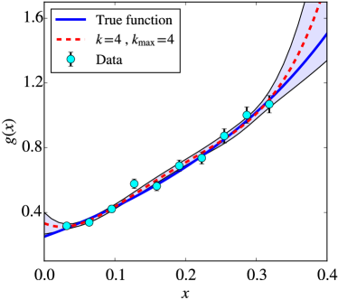
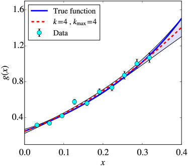
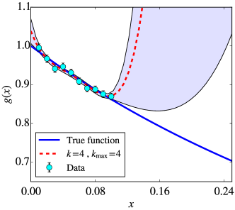
Figure 3 shows the results of a least-squares prediction where overfitting occurs at . The 1- error bands indicate that the leading behavior is poorly estimated, and that the fit is fine-tuned to reproduce the data where the error band is smaller. Figure 4 shows the same prediction made using Bayesian parameter estimates with the Gaussian naturalness prior. The true leading-order behavior (manifested at low ) and the prediction for above the last data point are much better reproduced, indicating that overfitting is avoided.
Table 3 shows the central values and 68% intervals obtained for the three leading coefficients, , , and from both the least-squares posterior pdf (left side) and the posterior pdf corresponding to the naturalness prior (right side). Results are shown for fits at different up to . The parameter estimates are obtained by MCMC integration and are consistent with the exact results in Tables 1 and 4 in Ref. Schindler and Phillips (2009a). The details of the exact calculations for these simple priors can be found in Ref. Schindler and Phillips (2009a). When computing the parameter estimates with MCMC, the error bars for the estimates were obtained from the ensemble of samples (see Sec. II.6). These results for the parameter estimates with their error bars are presented with a precision that is a conservative estimate of the error of the MCMC method itself; by increasing the number of samples in these calculations, the estimates will approach the exact ones in Ref. Schindler and Phillips (2009a). We note that Table 4 of Ref. Schindler and Phillips (2009a) contains an error: the logarithm of the posterior at the maximum parameter values quoted there for the Bayesian fit should be shifted down by one row. This mistake is corrected in the calculation that produced Table 3.
Our results confirm the finding of Ref. Schindler and Phillips (2009a): as the number of parameters is increased, the least-squares estimates of the leading coefficients degrade. As seen in Fig. 3 for the prediction, overfitting occurs as the coefficients become correlated in order to reproduce the data. This leads to large errors outside the fit region: compare the quality of the predictions there in Figs. 3 and 4.
The left side of the table uses the to indicate the quality of the fit, while the right side gives the evidence to show the relative extent to which the model describes the data (see Sec. III.4). The evidence here is controlled by , as discussed in Sec. III.4, and as we increase , the naturalness prior prevents fine-tuning by restricting the correlations between the leading coefficients and higher-order ones as we saw in the lower left of Fig. LABEL:sub@fig:triangle_D1_Gaussian. For any value of , the first two coefficients () are reliably extracted, with the posterior indicating when a coefficient is not well-determined by the data.
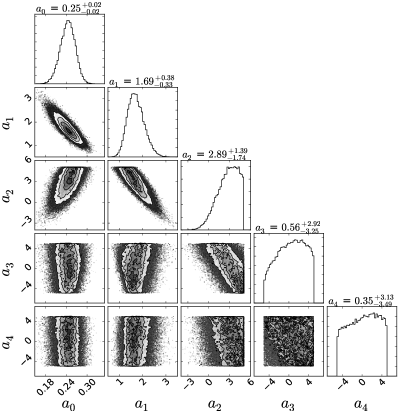
In Fig. 5, we show a corresponding projected posterior plot to Fig. LABEL:sub@fig:triangle_D1_Gaussian but using prior Set A′ (see Table 1) with . The marginalized posteriors on the diagonal for the higher-order coefficients become quite skewed and highly non-Gaussian; this would significantly complicate the determination of DoB intervals. However, the posteriors for these coefficients are primarily returning the prior—which in this case is flat. For the lowest-order coefficients, the posteriors are Gaussian-like and their modes and widths agree with those from Fig. LABEL:sub@fig:triangle_D1_Gaussian and the corresponding values listed in Table 3 up to when . We recover about the same two-parameter correlation plot for – as before, while those involving higher-order coefficients reflect details of the input prior. (Note that if we chose a distributed prior for and marginalized, these distributions would be significantly smoothed; using a delta function represents an extreme example.) Thus the meaningful results for this model are insensitive to the choice of prior; it is only necessary that the prior restrict the range of higher-order coefficients consistent with the expectations of naturalness.
III.3 Prior diagnostics
Our test cases make use of a fixed value of rather than marginalizing over a finite-width distribution for this naturalness parameter. This simplification is justified by using diagnostics for the prior that explore the sensitivity to .
In general one could marginalize over a range of values, and the posterior for , , when used in conjunction with the relaxation plot discussed next, is then useful for identification of an appropriate marginalization range for . The posterior will also signal the presence of unnatural coefficients (see Sec. V.1). This quantity can be expressed using marginalization and Bayes’ theorem as
| (30) |
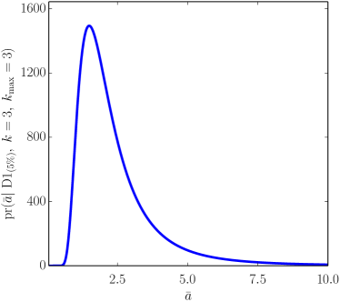
Note that this posterior can be obtained for different prior assumptions. The posterior is shown as a representative example in Fig. 6, in the case where the prior is Set C. The plot shows the region most likely for , which in this case implies natural coefficients.
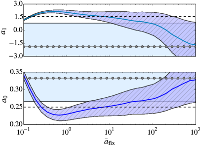
Another way to check the sensitivity of results to the naturalness parameter is to examine the parameter estimates when is fixed to various values . Hence we now employ prior Set C′ and vary from a small value to one large enough that the prior is effectively uniform. We use such results to create an relaxation plot (Fig. 7), which shows the projected posterior mean and width of different parameters as a function of a fixed value for . sets the width of the allowed region for the EFT parameters: Fig. 7 shows that too-small values of (e.g., of order 0.1) will bias the posterior severely, while large values relax to the least-squares (uniform prior) result.
Such “ relaxation” plots should be interpreted with care though, because a marginalization over when computing the coefficient posterior will weight different regions of in the integration according to the posterior . This can be seen by using the rule of marginalization to express the coefficient posterior from Eq. (27) in an alternate form:
| (31) |
where the first term in the integrand is the posterior for the coefficients given a specific and the second term is the posterior for that was calculated in Eq. (30). The result of marginalizing over therefore cannot directly be read from an relaxation plot. Figure 7 simply shows how the results change for fixed values of .
Ideally one finds (and marginalizes over) a slowly varying region in that is consistent with naturalness expectations; there should be little sensitivity to the endpoints of this region. There is sometimes a plateau in the dependence, but not always. If there is a plateau, and coefficient estimates are largely independent of in the region where is significant, then marginalization will be equivalent to fixing at an in this range. Taking a value for somewhat above the peak region for in the posterior then provides a choice which is not overly restrictive. In the present case, we conclude that the model in question will not be sensitive to details of how is marginalized in a wide region, and for simplicity we fix .
III.4 Model quality: Evidence
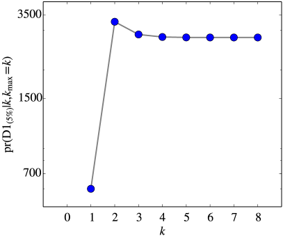
We discussed the evidence, which we define as , in general terms in Sec. II.5. In cases where the high-order coefficients are constrained by the naturalness prior, as in the situation reflected in Eq. (21), we expect saturation behavior of the evidence as parameters that are not well-constrained by the likelihood are added to the model. The evidence for a model at order marginalized over coefficients up to order is
| (32) |
where we have used the rule of marginalization from II.3, the fact that the prior for the naturalness parameter is independent of the truncation and marginalization orders.
Just as in the discussion of the impact of and on the posterior of in Sec. III.1, our evidence calculations are also controlled solely by . For any of our models calculated at with , Eq. (32) collapses to an integral over all the coefficients up to :
| (33) |
i.e., the value of is irrelevant so long as it is less than or equal to since all the higher-order coefficients up to must also be integrated. This result also applies for models which are nonlinear in the coefficients. For this reason we compute only the evidence calculated at , , e.g., as in Fig. 8. When the likelihood in Eq. (32) as a function of is more complicated, these integrals will not necessarily collapse so simply and the evidence may be affected separately by and , as discussed in Sec. III.1.
Comparing the evidence of models as parameters are added (or as we marginalize over more high-order coefficients) provides an ideal order-by-order comparison for the suitability of a model to describe the data Gregory (2005); Sivia and Skilling (2006). Therefore when we perform parameter estimation in our Bayesian framework, we also compute the evidence for each model to quantitatively decide how many terms can be extracted from the data, and how many higher-order terms to marginalize.
Figure 8 shows the evidence for to using prior Set C′ with . The evidence is also tabulated for each of these orders in Table 3. Comparing different orders, we see that the Bayes ratio , implying that the quadratic model is somewhat more favorable than the linear one.555We follow the empirical scale in Table 1 of Ref. Trotta (2008), for which the thresholds for weak, moderate, and strong evidence favoring one model over another are ratios of 3, 12, and 150, respectively. Comparing higher orders, the Bayes ratio for the to case is about 1, indicating that they are equally favorable. This we define as evidence saturation, based on the discussion in Sec. II.5, where going to higher order in the model does not improve the description of the data. When doing the parameter estimation for our examples, if coefficients are expected to be determined by the data, the order should not affect these estimates; any coefficients above order will essentially return the prior. However, verifying that this is true is an important part of the parameter estimation procedure. As emphasized in Ref. Lepage et al. (2002), simply truncating the fit at order amounts to taking a delta-function prior for all coefficients of higher-order terms, since it assumes they are precisely zero.
III.5 plots
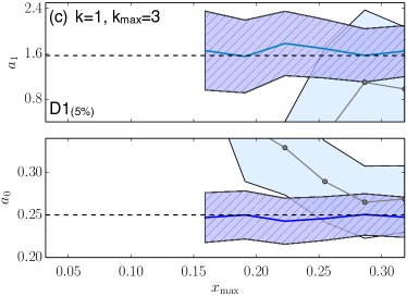
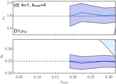
Variable plots show the projected maxima and widths of the parameters (which, for this problem, are the means and 1- errors) as a function of the maximum parameter value to which data are fit. In this way we examine the coefficients as we sequentially add data sampled at larger values of , where higher-order contributions become increasingly important. The effect on the computed posterior can be seen from Eq. (4), where the data at different values of form the residuals of the likelihood in Eq. (9), which goes into the coefficient posterior calculation. Plotting the evolution of the parameters as a function of shows the influence of each datum on the stability of the posterior in each dimension. Projected posterior plots such as those in Fig. 1 would be necessary to further analyze the correlations between orders at each value of .
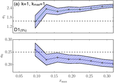
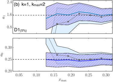
A series of such plots are shown in Fig. 9 for data set at four different fixed orders. The data set can be seen in Figs. 3 and 4 where we plot predictions from parameter estimates using different priors on the coefficients. We plot the parameter results as the order of the marginalization is increased, starting in Fig. LABEL:sub@fig:xmax_D1_M1 with (no higher-order coefficients) and going up to in Fig. LABEL:sub@fig:xmax_D1_M4. We plot the estimates with the naturalness prior as solid lines with error bands and compare these results with the least-squares results, plotted as lines with circles.
Some observations:
-
•
The plot illustrates underfitting: the linear model only works well for the most infrared data (here the smallest point only) and significantly deviates from the true result elsewhere. Consequently, the result for larger shows no stability. The prior for and is seen to be irrelevant here, and the least-squares results are the same as the estimates with the naturalness prior.
-
•
The plot with no prior shows overfitting for the lowest values of , as there are too many terms available for the fit data, given the size of the (simulated) experimental error. As increases, the least-squares result becomes reliable. With the naturalness prior included, there is stability for and over the entire range. This marginalization over is the key feature for stability with .
-
•
The plot shows that the uniform-prior results are off the scale for much of the displayed range, in strong contrast to the result with the naturalness prior, which gives stable central values and 1- errors. These naturalness-prior results are similar to the corresponding results when . These patterns continue—for both the uniform-prior and naturalness-prior results—when [shown in Fig. LABEL:sub@fig:xmax_D1_M4] and beyond (not shown).
This example illustrates the utility of using plots to check for instability with respect to the data range, which can signal underfitting and/or overfitting.
The stability with indicates that all high- (UV) effects have been sufficiently accounted for, and that adding more high- data does not improve the estimates. The value at which these particular extractions become stable with respect to corresponds to that at which the evidence saturates. In this example, stability with begins when , which is where the evidence saturates in Fig. 8. In fact, we will see in Sec. V.2 that plots can show stability when the evidence is past the saturation peak. This emphasizes the need to examine all the diagnostics before reaching a conclusion on the validity of the parameter estimation.
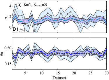
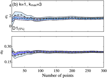
III.6 Multi-set and accumulation
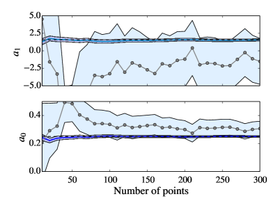
Multi-set [Fig. LABEL:sub@fig:D15_datasets] and accumulation [Fig. LABEL:sub@fig:D15_accumulated] plots are useful when there is enough data to subdivide it into a collection of smaller but (roughly) equivalent data sets. Multi-set plots provide a visualization of how fluctuations in the data affect the parameters. Figure LABEL:sub@fig:D15_datasets illustrates the fluctuations of the parameters and , estimated with the naturalness prior, as compared to the least-squares estimates, for the case . For 30 data sets sampled on the same grid with the same random error as , we compare the maxima and width of the projected posteriors for each coefficient. This plot illustrates how large the fluctuations in the coefficients are as the data fluctuates. The added restriction from the naturalness prior reduces both the spread in the calculated central values and the size of the coefficients’ error, compared to the result using the uniform prior.
Accumulation plots illustrate the utility of the prior when few data are available. Reading Fig. LABEL:sub@fig:D15_accumulated from left-to-right shows that when there is less data available, the naturalness prior increases the precision of the estimates. Once there is enough data the uniform prior and naturalness prior results do not differ since the likelihood is the dominant component of the posterior. However, the danger with a uniform prior is that overfitting can degrade the parameter estimation, even when there is a large amount of data, see Fig. 11. Even with a large data set the uniform prior on included coefficients—and -function prior on omitted coefficients—means care must be taken in choosing , so that neither overfitting or underfitting takes place. Bayesian parameter estimation avoids this delicate selection, because the estimates of the low-order coefficients are stable with respect to .
III.7 Residual plots
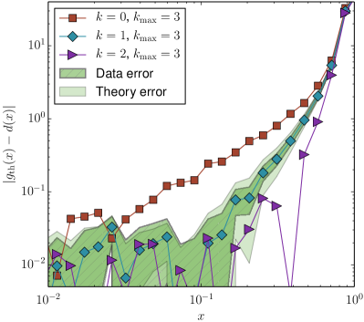
For sufficiently small values of the expansion parameter , the truncation errors for an EFT calculated to order should scale like the first omitted term (e.g., like if all orders are present). This can be tested by a log-log plot of the absolute values of the residuals (difference of prediction and data) as a function of . Plots of these type were introduced to analyze EFT behavior in Ref. Lepage (1997) and are commonly called “Lepage plots”. A successful realization of the EFT should ideally reveal a clear signal of power-law behavior, with the slope given by the order in the expansion, in an extended region of . This signal can be masked by data errors, particularly at low , and by still higher-order truncation errors as the breakdown scale is neared. A Lepage plot can manifest the different regions, help to disentangle regulator artifacts from errors due to truncating the EFT Hamiltonian, and, in principle, approximately determine the breakdown scale Furnstahl et al. (2015b).
We show an example of such a plot for Model D using in Fig. 12. The three sets of points are residuals at orders , 1, and 2, from a parameter estimation at . Data and theoretical error bands have been added for the residuals to help identify the crossover between the region where data errors mask the signal of the first omitted term and where the anticipated power-law behavior should be seen. In this example, the crossover occurs at successively higher values of , with at best a very narrow region of power-law behavior for .
In practice data are frequently sparse and too noisy to robustly discern from Lepage plots whether power-law exponents are in accordance with EFT expectations. A different type of error plot that avoids this problem compares theory residuals from different values of an EFT regulator scale (i.e., cutoff) rather than between theory and data Griesshammer (2015, 2004); Bedaque et al. (2003). Examples and further discussion of residual plots are given in Ref. Furnstahl et al. (2015b) and we do not consider them further in the present work.
IV The Parameter Estimation Process
IV.1 Overview
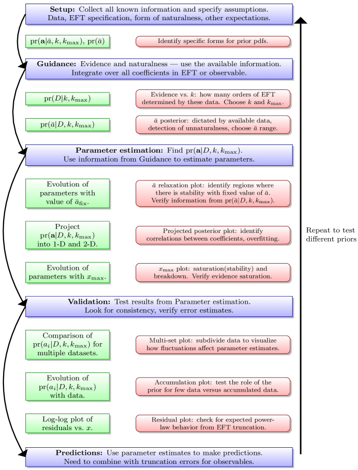
In Fig. 13, we present a possible flowchart for the full parameter estimation process, which orders and builds on the diagnostic tools described in the last section. The process starts with the Setup of the model and specification of all available information and theoretical expectations (including the form of the priors but not their widths), and ends with Predictions of observables from the fit parameters (or, more precisely, from the posteriors for the parameters). The intermediate steps are divided into Guidance, Parameter estimation, and Validation. In this section we consider each of these in turn, not exhaustively, but to highlight how individual diagnostics can offer different insights into parameter estimation for EFTs. We emphasize that while we have for clarity described the process as a forward flow, in practice one would backtrack if later diagnostics do not support earlier conclusions.
We choose another convenient model for these explorations:
| (34) |
with fixed . The Taylor expansion, which identifies the coefficients we seek to estimate, is
| (35) |
Note that the pole is at negative so that the radius of convergence is “hidden” in the data. This also means that the coefficients in the Taylor expansion have alternating sign. The magnitudes of the coefficients are up until , where they begin decreasing. We consider a variety of data sets, of varying precision, and with data over different ranges in and with different numbers of points. These sets are enumerated in Table 4 (and available in files in the supplementary material). We add a subscript to the label to indicate the percent relative error. Figures 14 and 15 show the underlying model function from Eq. (34), along with one data set . Both fits agree quite well in the region where there is data. But, outside that interval, the uniform-prior predictions in Fig. 14 show the consequences of overfitting. The result is not in agreement with the underlying function already a disappointingly small distance above the fit region. And the problems are not just at high : the overfitting reduces precision at low too. The Bayesian result in Fig. 15 does not suffer from these problems.
| Label | # of pts. | Grid | Spacing |
|---|---|---|---|
| H0 | 10 | linear | |
| H1 | 10 | linear | |
| H2 | 15 | linear | |
| H3 | 10 | quadratic | |
| H4 | 15 | linear |
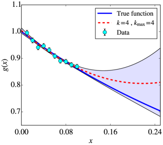
The data sets in Table 4 are representative of different situations that might be encountered in EFT parameter estimation. has very small errors and is sampled on a mesh where the expansion parameter is very small. is sampled over a small range of with a fairly large data error. expands upon the mesh by adding an additional 5 ultraviolet (UV) measurements to the mesh to probe the improvement of leading-order extractions when UV data are added. Finally, is an accurate data set measured on a quadratically spaced mesh (in the same range as ). This both simulates an application to EFT expansions with even powers only and results in a data set with several high-precision measurements at small . is used in Sec. V.2 as a case study of an EFT fit beyond its breakdown scale.
| Uniform prior | Gaussian prior | ||||||||
| dof | Evidence | ||||||||
| 0 | 0 | 20 | 0.920.00 | 0.920.00 | |||||
| 1 | 1 | 0.90 | 0.990.01 | 0.1 | 0.990.01 | 0.1 | |||
| 2 | 2 | 0.64 | 1.00.01 | 0.5 | 6.74 | 1.00.01 | 0.4 | 4.03 | |
| 2 | 3 | 0.74 | 1.00.02 | 1 | 9.830 | 1.00.01 | 0.4 | 4.03 | |
| 2 | 4 | 0.67 | 1.00.03 | 4 | 130100 | 1.00.01 | 0.4 | 4.03 | |
| 2 | 5 | 0.54 | 1.10.1 | 9 | 580400 | 1.00.01 | 0.4 | 4.03 | |
| 2 | 6 | 0.69 | 1.10.1 | 20 | 1902000 | 1.00.01 | 0.4 | 4.03 | |
| True values | 1.0 | 1.78 | 1.0 | 1.78 | |||||
| Uniform prior | Gaussian prior | ||||||||
| dof | Evidence | ||||||||
| 0 | 0 | 13 | 0.650.01 | 0.650.01 | |||||
| 1 | 1 | 2.3 | 0.890.03 | 0.1 | 0.890.03 | 0.08 | |||
| 2 | 2 | 2.3 | 0.950.05 | 0.4 | 0.6 | 0.950.05 | 0.4 | 0.951 | |
| 2 | 3 | 2.5 | 1.00.08 | 1 | 4 | 0.960.06 | 0.7 | 1.83 | |
| 2 | 4 | 2.9 | 0.920.1 | 3 | 20 | 0.970.06 | 0.7 | 1.83 | |
| 2 | 5 | 3.5 | 0.750.2 | 7 | 70 | 0.970.06 | 0.7 | 1.93 | |
| 2 | 6 | 4.0 | 0.130.5 | 20 | 200 | 0.970.06 | 0.7 | 1.73 | |
| True values | 1.0 | 1.78 | 1.0 | 1.78 | |||||
| Uniform prior | Gaussian prior | ||||||||
| dof | Evidence | ||||||||
| 0 | 0 | 29 | 0.530.01 | 0.530.01 | |||||
| 1 | 1 | 2.4 | 0.890.02 | 0.04 | 0.890.02 | 0.04 | |||
| 2 | 2 | 1.2 | 1.00.04 | 0.2 | 0.770.2 | 1.00.04 | 0.2 | 0.770.2 | |
| 2 | 3 | 1.3 | 1.00.1 | 0.5 | 1.61 | 1.00.05 | 0.5 | 1.41 | |
| 2 | 4 | 1.3 | 1.10.1 | 1 | 5.95 | 1.00.06 | 0.6 | 1.62 | |
| 2 | 5 | 1.3 | 1.00.1 | 3 | 20 | 1.00.06 | 0.7 | 2.02 | |
| 2 | 6 | 1.3 | 1.10.2 | 5 | 2350 | 1.10.06 | 0.7 | 2.22 | |
| True values | 1.0 | 1.78 | 1.0 | 1.78 | |||||
| Uniform prior | Gaussian prior | ||||||||
| dof | Evidence | ||||||||
| 0 | 0 | 380 | 0.680.00 | 0.680.00 | |||||
| 1 | 1 | 4.4 | 0.940.00 | 0.01 | 0.940.00 | 0.01 | |||
| 2 | 2 | 0.88 | 0.980.01 | 0.1 | 0.1 | 0.980.01 | 0.07 | 0.12 | |
| 2 | 3 | 0.73 | 0.960.02 | 0.2 | 0.9 | 0.960.01 | 0.2 | 0.8 | |
| 2 | 4 | 0.62 | 0.940.03 | 0.6 | 4 | 0.960.02 | 0.3 | 1 | |
| 2 | 5 | 0.58 | 0.900.05 | 2 | 10 | 0.960.02 | 0.3 | 2 | |
| 2 | 6 | 0.78 | 0.900.1 | 4 | 50 | 0.960.02 | 0.3 | 2 | |
| True values | 1.0 | 1.78 | 1.0 | 1.78 | |||||
Tables 8, 8, 8, and 8 each show the results from the Parameter estimation stage using the data sets enumerated above, which are generated at random and are not selected to be “typical” in any way. As a consequence, the impact of fluctuations is manifested. Without accounting for the errors, one might jump to false conclusions by naive comparisons to the true values. We see two examples immediately. First, the estimates for in Table 8 with the Gaussian prior are much closer to the true values than those in Table 8. But, the latter’s tighter 68% DoB limits say it is the more precise prediction; it is just chance that the extraction from the H1 data set results in a central value that is close as the DoB limits are quite wide. Second, in Table 8, the estimates with a Gaussian prior differ from the true values well beyond the quoted error bars. But, as documented below, this particular data set happened to have fluctuations in the data points, which leads to estimates for which the true value is outside the 68% DoB interval. This should not be a surprise; indeed, it is expected one-third of the time! The occurrence of a large fluctuation in provides a testing ground for our multi-set analysis (see Sec. III.6); this will reveal the impact of fluctuations on parameter estimates.
IV.2 Guidance: Exploring the prior, , and
The goal of the Guidance stage of our parameter estimation process is to take a particular data set and determine two aspects of the associated fit: the number of EFT parameters that can be reliably extracted and the range of naturalness parameters that should be used in that extraction. (Note: these procedures can be adapted to priors for other information.) The evidence illuminates the information content of the data with respect to the order of our fit. It is important to do the parameter estimation in the -region where the evidence has saturated, or else the estimates of those coefficients that can be determined will not be stable with respect to the order of marginalization . In Sec. III.4 it was discussed that for these model problems when , the evidence is controlled exclusively by . Therefore when we calculate the evidence, we do so for as we did in Fig. 8. For s not in the saturation region the coefficients are underfit—even in the presence of a naturalness prior. Meanwhile, the pertinent values of are indicated by the posterior , which shows the data’s content with respect to the naturalness of the coefficients.
The Guidance diagnostics are interrelated and should be compared for different prior assumptions—in this case we will compare Set C (or C′) and Set A as an example. As confirmed below, for Model H we can fix to a reasonable value of and the parameter estimates are largely insensitive to this choice. More detailed comparisons would be needed if results were more sensitive to the choice of prior. In the following we use the results in Tables 8, 8, 8, and 8 to evaluate what we learn from the Guidance stage.
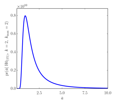
Small error, very small range. We first consider , a very accurate data set sampled at small values, and examine what the evidence and posterior plots tell us in advance of parameter estimation. The posterior in Fig. 16 uses prior Set C. It shows that the most likely value for given this information is about 1, and that choosing will not be overly restrictive. The evidence plot for Set C′ in Fig. 17 shows saturation at , with no real improvement from . This suggests that the limited range of this data set in means that we cannot extract information past the quadratic order (and that order will have limited information), and that we should marginalize over parameters . This conclusion is the same for different priors, and the evidence saturation behavior is compared for Set A and Set C′ in Fig. 17.
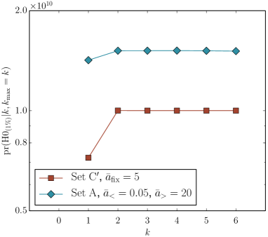
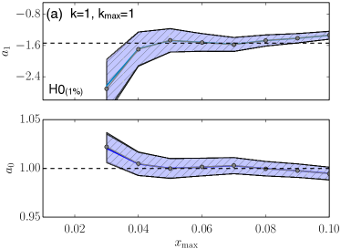
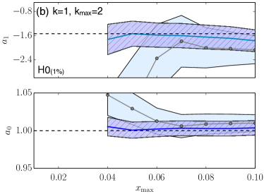
The expectations developed in the Guidance stage for are verified by the parameter estimates in Table 8. In particular, the results on the right side of the table using a Gaussian prior are consistent with determining successive orders with decreasing accuracy. The last coefficient determined by the data is , which has a large error, consistent with the evidence saturation. Higher-order coefficients simply return the prior.
It is instructive to compare to the results on the left side of the table, which are extracted using a uniform prior, i.e., assuming no prior knowledge of coefficient size. One might think that a high-quality data set with many points near should be dominated by the lowest-order terms, but these results show that the effects of fine-tuning are severe. In this case Table 8 shows that we have underfitting at , but, by the time we use for our fit, and have both acquired large (in absolute terms) central values. This overfitting only gets more marked as increases. In general the uncertainties allow and to be within the 68% (or, at worst 95%) DoB interval (once ) but the 68% interval is so wide in the case of that this statement is of little practical use. This is disappointing: one might have expected better from this low- (infrared) data. A projected posterior plot verifies that it occurs because and are highly anti-correlated, and there is nothing in this data set to pin down the value of .
At higher orders, plotting the uniform prior prediction, e.g., in Fig. 14, the fine-tuning (overfitting) problem is manifest. Similar results using the uniform prior for our other data sets are shown in Tables 8, 8, and 8, where generic underfitting/overfitting is also present. These issues make it clear that not including known information results in worse predictions, which can manifest in subtle ways. For example, the results for the uniform prior in Table 8 are not too far off from the true value but are in fact influenced by fine-tuning. The remaining significant error bar on shows that data in this narrow window does not have a good lever arm to accurately determine the slope of the underlying function at , a feature that is quantified by the evidence.
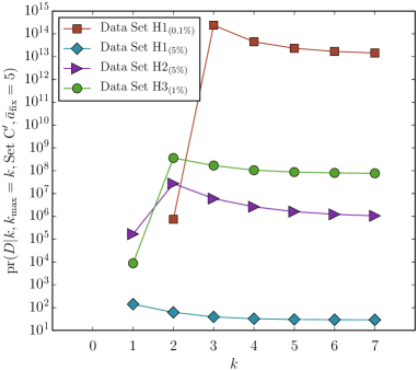
Large error, small range. In the case of , we might expect better constraints on from data that covers a wider but still small range of than . Fig. 18 shows a slight peak at and saturation at higher for . The interaction of the prior and likelihood is not as clean as in Eq. (21) when . By using only the order EFT where the evidence peaks rather than the saturation region, we are not including prior information that the EFT has higher-order coefficients—this results in a poor extraction, as is evident on the right of Table 8. Estimates should be made in the saturation region, and the coefficients extracted at lower orders become stable with respect to because we appropriately account for higher-order effects. The uniform-prior results for in Table 8 show that the result is not very good, but that in fact and have the same values for the /dof. Hence the lowest or the evidence peak are not reliable diagnostics of good parameter estimates—only when the evidence has saturated do the values of coefficients determined by the data cease to change with increasing .
For comparison, we also calculate the evidence for data set , which has 50 times smaller relative error than . For this highly precise data sampled on the H1 mesh from Table 4, the evidence saturates at in Fig. 18, indicating that there are limitations from where the data are sampled even if it is very accurate and precise. There is still a small peak in the evidence as there was in the case of 5% error.
Large error, larger range. has the same density of points as but has 5 extra points up to . Does the addition of 5 more UV points improve the lower-order estimates by constraining the higher-order ones better? Yes: Fig. 18 shows that the evidence with is now several orders of magnitude lower than the evidence in the saturation region near . The evidence is highest at but the estimates in Table 8 using a naturalness prior are not stable with respect to changing until the evidence saturates.
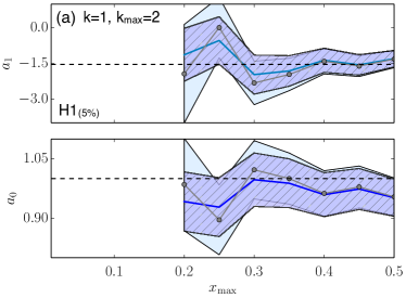
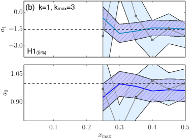
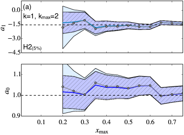
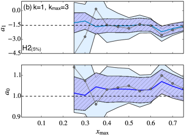
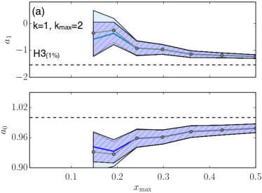
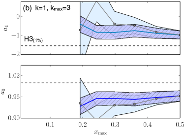
Small error, small range. Lastly, we examine , which samples the same region of as , but has more data points at small and has higher precision. The uniform-prior results are shown on the left side of Table 8, and we see the generic overfitting/underfitting. Figure 18 shows saturation at for this set. Compared to the evidence for , the decisiveness of the evidence at to is better. Turning to parameter estimation results using prior Set C′ on the right of Table 8, the extraction stabilizes as we enter the saturation region but the results do not seem consistent with the true values. This is not a failure, however; this particular data set is one of the 32% of data sets that will not produce LECs in the 68% band. The extraction is driven by the lowest- data point so that it is less than the true value, . We will discuss this data set further when considering multi-set plots below.
Summary. A uniform prior (least-squares method) is limited to the information in the data sets themselves. Whenever lower-order coefficients are correlated with higher-order ones, there will be underfitting of coefficients associated with the last included order—and overfitting of lower-order coefficients. While high-precision data can ameliorate the situation for a few coefficients, the potential of such a data set is still under-realized in a least-squares analysis. More generally, such difficulties cannot be avoided by choosing a particular domain for the fit.
The Bayesian procedure is much more effective but is still constrained by the limitations of the data set, and these limitations are quantifiable using the evidence. Using a wider region, but with less precise data, decreases the accuracy of the determination markedly. ( is determined with essentially the same accuracy from and .) The decrease in the accuracy of is not as bad in and as , because some of the loss in data precision is made up by the increased lever arm. All three data sets suggest that only a precise data set, over a wide range of , will be able to give unambiguous information on . Perhaps most notably, in each case, , , and , both the central values and 68% DoB intervals stabilize with once . Those stabilized results are consistent with the underlying values of all of , , and .
IV.3 Parameter estimation: analyses
For the Parameter estimation step in the process, the principal diagnostic is always the projected posterior plot, which illuminates the correlations and shows features such as which parameters are dominated by the prior. We have already examined examples of projected posterior plots and associated tables of parameter means and standard deviations, so here we focus instead on the added utility of plots. These track the evolution of parameter estimates as the data set is built up sequentially with more and more high- (UV) data, thus making it clear that choosing ranges of data to fit certain orders in the EFT may omit important information.
Small error, very small range. We saw in Fig. 17 that evidence saturation for occurs at , which is slightly favored over . But, Table 8 showed that, while the posterior contains some information on , it is largely undetermined. Therefore we explore the results (the first two coefficients), marginalizing over higher coefficients for . Figure LABEL:sub@fig:H01_xmax_k1_kmax1 shows the , plot. Here the uniform and prior Set C′ parameter estimates overlap and are not stable with increasing , indicating underfitting. When we marginalize to , where the evidence saturated, in Fig. LABEL:sub@fig:H01_xmax_k1_kmax2, the naturalness prior parameter estimates are stable with . The uniform-prior results are not and overfitting occurs, especially for small . Once , the uniform prior error bars encompass the true value but are significantly larger than the naturalness results. As is increased further into the saturation region, the parameter estimates with the naturalness prior continue to be stable with (not shown).
Large error, different ranges. Turning to and , which are sampled at larger ranges of with larger errors, we explore the behavior at values near the evidence saturation. Figures LABEL:sub@fig:H15_xmax_k1_kmax2 and LABEL:sub@fig:H15_xmax_k1_kmax3 show the results at with repectively for . In light of the evidence in Fig. 18, is approximately in the saturation region while does not account for enough higher orders. At the estimates at the largest overlap with the uniform-prior results, while the corresponding estimate for is slightly better. The results for are also fairly stable with , consistent with the evidence saturation.
For , with extra UV data, we show the , results in Figs. LABEL:sub@fig:H25_xmax_k1_kmax2 and LABEL:sub@fig:H25_xmax_k1_kmax3, which again explores the transition region near evidence saturation seen in Fig. 18. As we saw for , the estimates are not stable with until when the evidence truly saturates. In particular the final estimates with the largest in Fig. LABEL:sub@fig:H25_xmax_k1_kmax2 significantly underestimate the error in .
Small error, small range. The evidence for in Fig. 18 clearly saturates. We compare both , just showing the first two coefficients (), but not because it is in the underfitting regime. Surprisingly perhaps from the perspective of the evidence, in Fig. LABEL:sub@fig:H31_xmax_k1_kmax2 still gives underfitting and for no is the estimate consistent with the true parameter to the 1- level. Even for low , underfitting still occurs. But the essential feature here is the absence of stability with respect to , not that the 68% DoBs miss the true parameter values. In contrast, for , shown in Fig. LABEL:sub@fig:H31_xmax_k1_kmax3, there is stability with , even as the uniform-prior results begin overfitting. But, even here, the 68% DoB intervals miss the true value. Such “occasional misses” are, though, consistent with a statistical interpretation of these error bands.
Summary. Using plots rather than a fixed range of data provides valuable insight into the parameter extraction. They establish the region of that provides stable predictions, help to identify where in new information on coefficients stops, and confirm the evidence saturation from the Guidance.
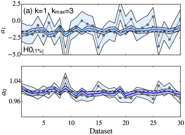
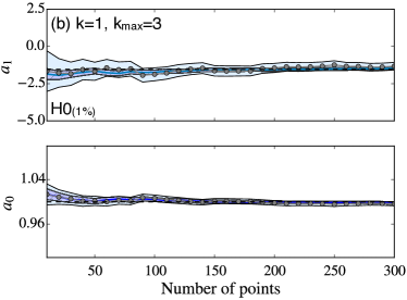
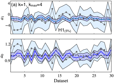
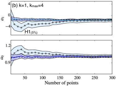
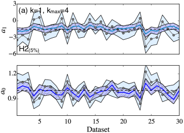
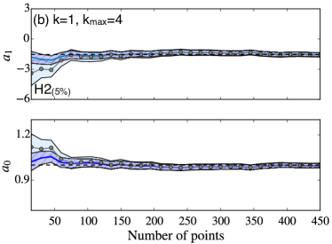
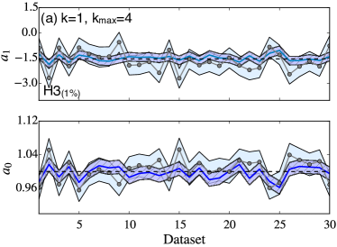
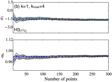
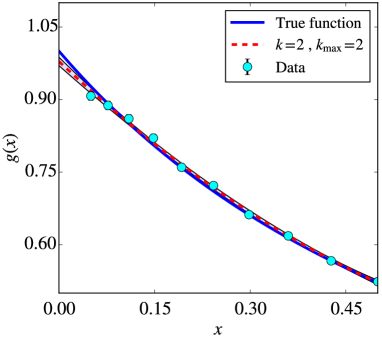
IV.4 Validation: Multi-set analysis
Finally, for the Validation step we focus on how fluctuations in data affect our results as well as how the errors in the available data limit parameter estimation. We posit that some larger set of measurements for our model is available, which we divide into smaller subsets and use to perform the parameter estimation to see the effects of statistical fluctuations (multi-set plots outlined in Sec. III.6). We also take these data sets and build them up sequentially to see how much data at that error level is needed to produce precise estimates (accumulation plots outlined in Sec. III.6).
Small error, very small range. Figure LABEL:sub@fig:H01_datasets_k1_kmax3 shows a multi-set plot for at with , which is well into the evidence saturation region. As overfitting occurs with the uniform prior, data fluctuations lead to fluctuations in the coefficients with large errors. The results using the naturalness prior have a smaller spread about the central value and smaller error bands. As is increased, the overfitting and coefficient fluctuations in the uniform prior case become even more severe, while the results with the naturalness prior are insensitive to increasing . Figure LABEL:sub@fig:H01_accumulated_k1_kmax3 shows how the estimates improve as more data are accumulated (in sets of 10 sampled the same way as ). Even with 300 points, the uniform prior results are not as precise as the naturalness prior results. The advantage of extra prior information is more in evidence in the top panel with , where the uniform prior error bands are much larger.
Large error, small range. The multi-set plot for is shown in Fig. LABEL:sub@fig:H15_datasets_k1_kmax4, this time for with , which is in the saturation region. Compared to , the fluctuations of estimates are much larger, due to the larger data error and sparser mesh, while the uniform-prior results are fluctuating even more due to overfitting. The accumulated results for the uniform prior in Fig. LABEL:sub@fig:H15_accumulated_k1_kmax4 are not consistent at the 1- level until about 150 points—and even there they still have errors that are larger due to different input information. The naturalness prior results are consistent with the true value even for only 10 points, but the error in the estimates does not decrease much as more data are added. Any further increase in precision is limited by the range of the data and the fluctuations in it.
Large error, larger range. The multi-set and accumulated results for are shown in Figs. LABEL:sub@fig:H25_datasets_k1_kmax4 and LABEL:sub@fig:H25_accumulated_k1_kmax4 for , . Compared to , the fluctuations between data sets in Fig. LABEL:sub@fig:H25_datasets_k1_kmax4 are not as large for either prior, but the naturalness prior reduces the spread. The accumulated results in Fig. LABEL:sub@fig:H25_accumulated_k1_kmax4 show that the prior improves the results until there are about 75 data points available and the results with different priors become the same. However, for larger values of the uniform prior result will not converge to the Bayesian one as well as it does for , as we saw for Model D in Fig. 11.
Small error, small range. The multi-set plot in Fig. LABEL:sub@fig:H31_datasets_k1_kmax4 for the first two parameters given , marginalized to , show tight error bands compared to the previous results using 5% error data sets, as would be expected because of the smaller 1% relative error in the data. The estimates in Fig. LABEL:sub@fig:H31_datasets_k1_kmax4 for the naturalness prior fluctuate statistically about the true value. Before, the results in the right-hand-side of Table 8 showed that the 68% interval missed the true parameter values, and a plot of results from that estimation in Fig. 27 at (in the saturation region) shows a resulting prediction from that data set. Fig. LABEL:sub@fig:H31_datasets_k1_kmax4 confirms that this was merely a result of the random error in that data set. This is important to keep in mind: the available physical data could lead to this type of estimate in an EFT. Thus statistically meaningful error bars are important so that resulting predictions have a true significance based on the data. The accumulated results in Fig. LABEL:sub@fig:H31_accumulated_k1_kmax4 show that even with just two data sets at this value of , the naturalness and uniform-prior results become the same.
Summary. The multi-set plots let us compare the impact of fluctuations on results using different prior information. In some cases the accumulated results can provide a sanity check that sufficient data will overwhelm the prior. The accumulated results also illustrate that data errors can severely limit what can be extracted from even a large amount of data when overfitting occurs. Using prior naturalness information about the coefficients can help even when many data are available.
IV.5 Predictions
After the Validation stage of Fig. 13, the posteriors for the LECs are available to make predictions of observables, with consistent propagation of data and theory uncertainties. Additional full loops in the flowchart may be appropriate to explore the impact on these predictions of different priors. In addition, we emphasize that truncation errors for predicted observables must be included for a full uncertainty quantification. We will not consider the Predictions stage further here, but reserve it for applications to actual EFTs in future work.
It should be evident that the Bayesian framework we advocate is far from automatic; there are many pitfalls along the way, but this is the nature of the problem. The simple case studies considered here illustrate some general truths about parameter estimation for EFTs: the size of data errors and the range of available data make a big difference; fluctuations happen; only so much information is available and the Bayesian evidence is necessary to quantify it. We have given examples of how the multiple tools we have outlined can be used together to optimize the extraction of the LECs and the uncertainty quantification. But we recognize the additional burden on the practitioner, which can introduce a significant and potentially prohibitive computational load. An important topic for further study is to what degree one can lighten this load while still working within the Bayes framework to provide robust statistical error bars (e.g., as in Ref. Higdon et al. (2015)). We caution that taking too many shortcuts may lose information from the data that could improve your LECs.
V Additional Case Studies
In this section we consider an additional set of parameter estimation case studies, which highlight some particular difficulties that may be encountered in EFT applications. Our philosophy is that validating the procedures and testing the diagnostics with model problems (which at the least means analyzing the EFT with synthetic data), where we can explore a full range of issues in fitting LECs with known answers, is essential before turning to optimizations from real data. The following examples serve as prototypes for behavior we expect to see in “real-world” cases.
V.1 Blind test: detecting unnaturalness
We performed several different blind tests of the procedure of Sec. IV to verify that already knowing the answer has not been causing confirmation bias in our analyses. For example, one might worry that our use of a naturalness prior by construction could guarantee that we will always find natural LECs unless we were already aware of unnatural coefficients. The corresponding blind test, described below, included an unnatural coefficient at a particular order, but the only information provided to the tester was a set of data points and a specification of the basis functions (the model EFT). The procedure set up in Sec. IV was applied to estimate the parameters of the model problem.
The first signals of unnaturalness should be detected in the Guidance stage, where the pdf of the naturalness parameter for the given prior choice is explored in the posterior pdf of : . During the Parameter estimation stage, an observation of unnaturalness should be confirmed by the evolution of the parameters with fixed (using prior Set C′ or A′), that is, the estimates will vary rapidly for expected natural values of , but will stabilize once is larger.
The case study we present here is a simple modification of Model D from Sec. III. In particular, an unnatural coefficient was added to the model of Eq. (23):
| (36) |
which therefore has the same Taylor series as in Eq. (23) except for an unnatural coefficient at third order in , altering the convergence rate—but not the convergence radius—of the expansion. Note that this is a somewhat extreme example because the unnaturalness is very large and occurs at a high order in the expansion. We refer to this as Model . We consider a data set that consists of 10 points sampled in the range .
| Uniform prior | Gaussian prior | ||||||||
| dof | Evidence | ||||||||
| 0 | 0 | 100 | 0.470.01 | 0 | 0.470.01 | ||||
| 1 | 1 | 9.9 | 0.130.01 | 3.80.1 | 7.5 | 0.130.01 | 3.80.1 | ||
| 2 | 2 | 2.2 | 0.280.02 | 0.300.5 | 132 | 5.1 | 0.280.02 | 0.350.4 | 132 |
| 2 | 3 | 2.4 | 0.250.04 | 1.31 | 4.19 | 5.4 | 0.270.03 | 0.810.7 | 8.65 |
| 2 | 4 | 2.4 | 0.350.1 | 3.13 | 6340 | 5.4 | 0.260.03 | 0.880.8 | 8.25 |
| 2 | 5 | 2.9 | 0.360.1 | 3.78 | 75100 | 5.4 | 0.260.03 | 0.920.8 | 8.15 |
| 2 | 6 | 0.73 | 0.540.3 | 5520 | 1300400 | 5.4 | 0.260.03 | 0.880.8 | 8.35 |
| True values | 0.25 | 1.57 | 2.47 | 0.25 | 1.57 | 2.47 | |||
Beginning with the Guidance stage, we compute the evidence of at several different orders and compute the posterior for . Looking at the evidence on the right-hand side of Table 9 for Set C′, we see that saturation occurs at , but that the ratio to is not much greater than unity. Therefore, we expect that the first three coefficients—, , and —should be determined. It is likely that the unnatural coefficient’s value can not be obtained with any real precision, making this a bastard of a blind test.
The posterior for using prior Set C is shown in Fig. 28 for . This posterior indicates that the most probable values for lie in a wide range peaked around , with a long tail extending to much larger values. This is a clear signature of unnaturalness. Choosing will likely cause the parameter estimates to be distorted by overly restricting the prior. We therefore choose in the extractions of Table 9 to avoid restricting the parameter space too much.
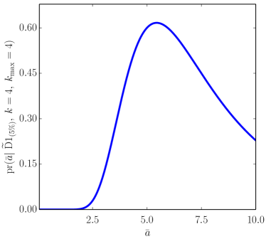
Unnaturalness is further confirmed during the Parameter estimation stage. Figure 29 shows how the first three coefficients, which should be rather well constrained by the data, change as a function of using prior Set C′. Without the guidance of the dashed lines indicating the true values of the underlying expansion, there is a strong indication that is about 10, while the first two coefficients are approximately natural. The evolution plateaus between of about 5 to 100, after which it rapidly transitions to the least-squares result.
It is also difficult to see where the unnaturalness is present in the expansion. In fact, if we did not marginalize over and with , the results for these coefficients corresponding to that row in Table 9 are and . The unnaturalness is present in the estimate of , which is, however, rather poorly determined. The correlations inherent in a (naive) polynomial fit result in the unnaturalness being shared between and its neighbors. I.e., the presence of unnaturalness can distort the fit result of other coefficients which are natural. In this example it is—absent high-quality data in an appropriate region of —difficult to disentangle the specific order at which the one unnatural coefficient occurs.
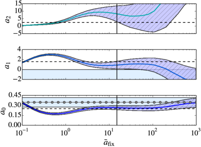
In spite of this, unnaturalness in the EFT fit can be identified using the procedure of Sec. IV: there are clear signals in the Guidance and Parameter estimation stages. Disentangling at which order the unnatural LEC appears in the expansion is difficult, and the presence of an unnatural LEC can distort LECs which are in fact natural. With more information, such as knowing which orders have natural and unnatural contributions, we could update the prior pdfs for accordingly.
V.2 Data past breakdown of theory
An EFT expansion parameter will typically take the form of a ratio of scales that becomes one at the breakdown scale, where dynamics not explicitly included in the EFT appear. The analogous theory breakdown for our models is at the radius of convergence of the expansion. We explore estimating the parameters of Model H from Sec. IV using a data set sampled past the theory breakdown. In this case we have data set , which is described in Table 4. We have now three points sampled at where the expansion does not converge. Since the pole for Model H is at negative , the function does not exhibit singular behavior at and so the breakdown is “hidden”.
Our aim is to determine signatures of the EFT breakdown using this data set, i.e., determine whether the procedure of Sec. IV is sensitive to it. We compute the evidence and posteriors to complete the Guidance stage. The posteriors do not indicate unnaturalness for any order, and so we compute the evidence for using .
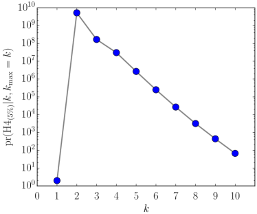
| Evidence | |||||||
| 0 | 0 | 0 | 0.310.00 | ||||
| 1 | 1 | 1.5 | 0.690.01 | 0.340.01 | |||
| 2 | 2 | 8.8 | 0.860.03 | 0.780.06 | 0.230.03 | ||
| 3 | 3 | 1.1 | 0.900.04 | 0.980.2 | 0.490.2 | 0.100.1 | |
| 4 | 4 | 2.1 | 0.980.07 | 1.60.4 | 2.00.9 | 1.40.8 | 0.380.2 |
| 4 | 5 | 5.2 | 0.970.08 | 1.50.7 | 1.52 | 0.593 | 0.152 |
| 4 | 6 | 1.4 | 0.970.08 | 1.50.7 | 1.52 | 0.313 | 0.703 |
| True values | 1.0 | 1.78 | |||||
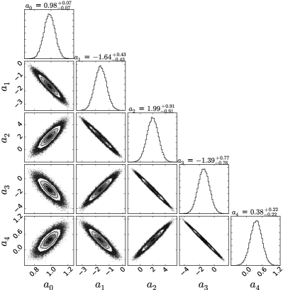
Figure 30 shows the evidence values. Compared to the saturation behavior using data sets sampled at smaller values, the behavior of the evidence is strikingly different. The evidence decreases exponentially with increasing order of the expansion, and the pattern continues without saturating past the highest order shown in Fig. 30. We turn to the Parameter estimation stage to further examine the estimates with increasing . Table 10 shows the parameter estimates for the coefficients up to . Although the results for and are fairly stable, the results for and beyond are not stable as we saw in other test cases. Examining the projected posterior plot in Fig. 31 at gives us a clear picture of the interaction of the likelihood with the prior in this case. We see tight correlations between coefficients remain in spite of the naturalness prior, unlike before where higher-order coefficients became almost uncorrelated with leading-order coefficients.
We continue with the Parameter estimation stage, examining the plots for , which compare the prior Set C′ results with the uniform-prior results. Figure LABEL:sub@fig:H45_xmax_k1 shows the plot for , and we continue up to in Fig. LABEL:sub@fig:fig:H45_xmax_k4. In Fig. LABEL:sub@fig:fig:H45_xmax_k2, which corresponds to the evidence peak in Fig. 30, the results are not stable with respect to , and without relying on the dashed lines of the true values, no conclusive statement can be made. However, once we go to order in Fig. LABEL:sub@fig:fig:H45_xmax_k4, the results are fairly stable with respect to , but and remain significantly correlated with the higher-order coefficients.
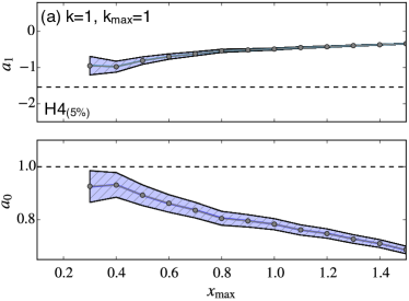
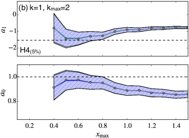
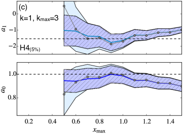
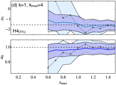
When we have data over a large range in the expansion parameter, the correlations between lower-order and higher-order coefficients may not be washed out by the naturalness prior. Since we have data at values of where terms at different orders have similar contributions, the higher-order coefficients are not uniquely determined, resulting in large correlations and delicate cancellations. The likelihood should be further analyzed using singular value decomposition (SVD) to see the effects of the data. The example here shows that with enough low- data, the leading behavior can still be extracted, but that further analysis is necessary to find the best way to utilize the available data.
V.3 Nucleon mass in PT
Lattice calculations of observables near the physical pion mass are computationally expensive. Therefore, there is a need for extrapolations to the physical point, and chiral perturbation theory (PT) should be an ideal tool for extrapolations Bernard (2015). However, the lack of lattice data near (or below) the physical point means that extracting the coefficients in an expansion about zero pion mass can be difficult. It often turns out that we need to disentangle contributions of different orders in the PT expansion at a pion mass where the expansion parameter is not particularly small. In this section we confront such difficulties, by applying our generic EFT tools for parameter estimation to chiral extrapolations from synthetic lattice data for the nucleon mass as a function of the pion mass, .
At a technical level these PT expansions differ from the model problems described above since there can be several LECs at a single order, due to the possibility of different non-analytic functions multiplying the same overall power of . Orders can also be skipped, e.g., there is no term in the PT expansion of the nucleon mass. Therefore in this section we no longer refer to and , replacing them by and , which indicate PT orders, rather than numbers of LECs.
Following previous work in Ref. Schindler and Phillips (2009a), we fit the LECs of the expansion for the nucleon mass from SU(2) PT. We are particularly interested in the first two low-order coefficients. The leading coefficient is the nucleon mass in the chiral limit, and the term at chiral order is related to the pion-nucleon sigma term Bali et al. (2013).
The nucleon mass expansion in terms of the intrinsic scale is given by Schindler and Phillips (2009a):
| (37) |
where is the pion mass, is the renormalization scale for the loop contributions, and the expansion is up to sixth order in PT. Since the expansion is about zero pion mass, ideally we would determine the free parameters from data sampled at small quark masses. We explore synthetic lattice data sampled at various ranges of , investigating the feasibility of chiral extrapolations.
We can define scale-invariant LECs in this expansion by expressing the basis functions in terms of , absorbing the dependence into the coefficients. If we wish to take into account the contributions at that order using marginalization, it is sufficient to account for the dominant power . However, we do not make this approximation here, instead accounting for all terms in the chiral expansion up to sixth order, as written in Eq. (37).
Following Ref. Schindler and Phillips (2009a), we generate synthetic data by taking MeV and computing values for the LECs of Eq. (37) at the renormalization scale with MeV. These constants are given by (with and the relevant dimensions of [GeV]-n) Schindler and Phillips (2009a, b)
| (38) |
At this value of these LECs are approximately natural, and henceforth we use it in our calculations.
With these constants chosen, we add to the chiral expansion a model-dependent term that turns on slowly and becomes strong around MeV which simultaneously turns off the expansion. The synthetic data are generated from the function Schindler and Phillips (2009a)
| (39) |
This model-dependent term has the form
| (40) |
where the values GeV and are selected following Ref. Schindler and Phillips (2009a). The function that controls the dominance of each term in Eq. (39) is Schindler and Phillips (2009a)
| (41) |
Figure 33 shows a plot of the function of Eq. (39) from which synthetic data are sampled compared to the chosen chiral expansion alone and a data set .
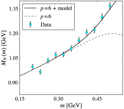
We consider three data sets to represent different scenarios for lattice simulations. The pion mass meshes at which each was sampled are enumerated in Table 11. We first examine two realistic cases of synthetic data, and , which are sampled at and above the physical pion mass with a 1.5% relative error. After seeing the limitations of data that simulates the current limitations of lattice calculations we explore an idealized set, , where the sampling begins at MeV.
| Label | # of pts. | Grid | Spacing |
|---|---|---|---|
| MN0 | 11 | GeV | linear |
| MN1 | 11 | GeV | linear |
| MN2 | 11 | GeV | linear |
| Uniform prior | Gaussian prior | ||||||||
| dof | Evidence | ||||||||
| 0 | 0 | 35 | 2.10.01 | 0 | 2.10.01 | ||||
| 2 | 2 | 0.85 | 1.80.02 | 0.820.04 | 4.1 | 1.80.0 | 0.820.04 | ||
| 3 | 3 | 0.96 | 1.80.04 | 0.820.4 | 0.0020.4 | 3.0 | 1.80.0 | 0.820.3 | 0.000.4 |
| 3 | 4 | 0.91 | 1.60.3 | 7.710 | 2760 | 1.4 | 1.80.1 | 2.11 | 1.24 |
| 3 | 5 | 0.98 | 5.14 | 490600 | 58006000 | 6.9 | 1.80.1 | 1.92 | 0.974 |
| 3 | 6 | 0.53 | 20001000 | 8.85 | 2.41 | 3.9 | 1.80.1 | 1.82 | 0.834 |
| True values | 1.76 | 1.92 | 1.41 | 1.76 | 1.92 | 1.41 | |||
| Uniform prior | Gaussian prior | ||||||||
| dof | Evidence | ||||||||
| 0 | 0 | 51 | 2.20.01 | 0 | 2.20.01 | ||||
| 2 | 2 | 1.4 | 1.80.02 | 0.890.04 | 1.4 | 1.80.02 | 0.890.04 | ||
| 3 | 3 | 1.4 | 1.90.1 | 0.490.4 | 0.370.3 | 1.8 | 1.90.1 | 0.470.4 | 0.380.3 |
| 3 | 4 | 1.7 | 2.60.7 | 2120 | 8980 | 3.1 | 1.80.1 | 0.982 | 0.104 |
| 3 | 5 | 1.2 | 3720 | 27001000 | 2.51 | 1.2 | 1.80.1 | 0.612 | 0.494 |
| 3 | 6 | 0.20 | 4508000 | 1.32 | 3.15 | 6.0 | 1.90.2 | 0.142 | 0.874 |
| True values | 1.76 | 1.92 | 1.41 | 1.76 | 1.92 | 1.41 | |||
| Uniform prior | Gaussian prior | ||||||||
| dof | Evidence | ||||||||
| 0 | 0 | 5.4 | 1.820.01 | 0.015 | 1.820.01 | ||||
| 2 | 2 | 1.1 | 1.730.02 | 2.20.33 | 4.0 | 1.730.02 | 2.20.3 | ||
| 3 | 3 | 1.2 | 1.710.03 | 3.72.7 | 4.78 | 3.3 | 1.720.02 | 2.41.4 | 4 |
| 3 | 4 | 1.3 | 2.10.3 | 140110 | 20002000 | 3.1 | 1.720.02 | 2.51.4 | 4 |
| 3 | 5 | 1.9 | 1.55 | 4505000 | 160002 | 3.1 | 1.720.02 | 2.51.4 | 0.604 |
| 3 | 6 | 0.25 | 15001000 | 4.9 5 | 3.7 4 | 3.1 | 1.720.02 | 2.51.4 | 4 |
| True values | 1.76 | 1.92 | 1.41 | 1.76 | 1.92 | 1.41 | |||
We first analyze data sets that emulate currently available lattice calculations. is sampled with the lowest -value near the physical point MeV up to MeV, where there is noticeable contribution to the generated data from the model-dependent part. In the Guidance stage, we consider the evidence in Table 12, which peaks at but decreases by two orders of magnitude from to . There is no indication of unnaturalness in the posteriors at any order.
We proceed with the Parameter estimation, looking for stability with increasing orders of the extraction in accordance with the evidence calculations from the Guidance stage. Even though the evidence peaks at , the parameter estimates in Table 12 do not stabilize at that order. In fact, they do not stabilize until . The result for is well-determined and consistent with the true value at the 1- level, but is rather poorly determined, although the estimate is consistent with the true value to within the quoted error estimates. With the data currently available to practitioners, lattice extrapolations will likely be difficult past the leading order.
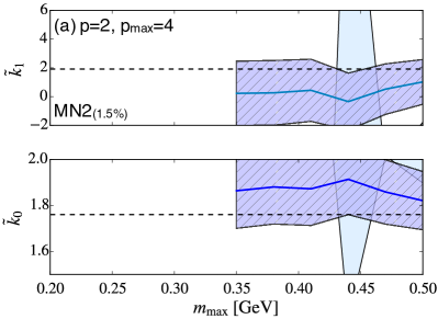
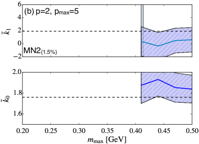
We also examine the results of parameter estimation from . A plot of this data set is shown in Fig. 33 compared to the underlying nucleon mass function used to generate the data and the chiral expansion up to sixth order. The data are sampled up to a region where the model-dependent term becomes significant. Table 13 shows the evidence and parameter estimates using prior Set C′ compared to the uniform-prior results. The evidence shows no pleasing saturation behavior for this data set, perhaps indicating that we are sampling too near the breakdown of the expansion, as in Sec. V.2. However, there is no indication of unnaturalness in the posterior at any order. It appears that the results are not stabilizing as the order is increased, but comparing the plots of Fig. LABEL:sub@fig:MN2_xmax_k2_kmax4 and Fig. LABEL:sub@fig:MN2_xmax_k2_kmax5 at and respectively, the final results look consistent and stable with . The coefficients are reproduced at the 1- level with rather large errors. Even extracting the leading coefficient in this case is very difficult, with the next-order coefficient mostly undetermined. As in Sec. V.2, it is not possible to extract conclusive results where the expansion cannot describe the data well.
We finally examine , which is an idealized set sampled at significantly smaller pion masses than the previous two sets. We first compute the evidence and naturalness parameter posteriors to complete the Guidance stage for . Figure 35 shows the posterior for assuming prior Set C at chiral order , . We see no indications of unnaturalness in this data set, and again choose for prior Set C′. Computing the evidence using this choice, the results in Table 14 show that the evidence reaches saturation at about , where the values peak slightly, and then levels off at higher orders. The expectation is that only two coefficients will be determined by this data. Even in the unrealistic case where we have high-quality data below the physical pion mass, we do not expect to determine more than two LECs in the chiral expansion.
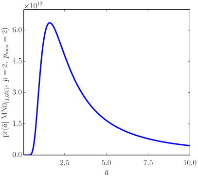
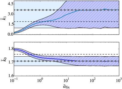
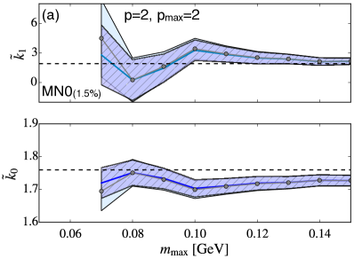
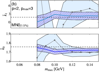
Turning to the Parameter estimation, the results in Table 14 show that the data set MN0(1.5%) leads to an underestimate of the parameter compared to the true value, while has a better central value than was obtained from , albeit still with a sizeable uncertainty. The underestimation of is another example of the effect of fluctuations in the data. The sizeable error on indicates that, although the coefficient is fixed by the data, the precision we can obtain is quite limited. At order , which was the saturation order from the Guidance stage, the naturalness-prior parameter estimate for is spuriously precise—likely a result of underfitting of at this order. This illustrates the importance of going well into the region of where the evidence flattens out, in order to eliminate the possibility of underfitting. Examining the results using a uniform prior in Table 14, we see very similar parameter estimates as for the naturalness prior at , but any attempt to check the stability of that result by going to higher chiral order leads to extreme overfitting: by the time we reach , where there are ten total coefficients, least squares is producing central values and 68% intervals of order or . The additional information imparted to the fit by the naturalness prior is essential to meaningful parameter estimation once we go to . And going to is necessary in order to achieve stability of the extraction with chiral order.
The plots in Figs. LABEL:sub@fig:MN0_xmax_k2_kmax3 and LABEL:sub@fig:MN0_xmax_k2_kmax2 also show that stability with respect to the pion-mass interval over which data is fit is only achieved at order —in accordance with the inference from Table 14 that there is underfitting at . The relaxation plot in Fig. 36 confirms a naturalness parameter between 1 and about 5; this is consistent with the guidance from Fig. 35.
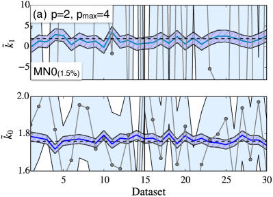
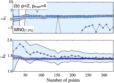
Finally, the Validation stage gives some indication of the effects of fluctuations in the data set, where we compare many independent samplings on the grid in the multi-set plot of Fig. LABEL:sub@fig:MN0_datasets_k2_kmax4, where we choose . The fluctuations in the results using the uniform prior are severe, and the results using prior Set C′ fluctuate much less. Comparing the results for the first two coefficients at with these 30 independent data sets to the previous estimates with our single data set , we conclude that the naturalness prior result for in Table 14 is consistent with the fluctuations seen in Fig. LABEL:sub@fig:MN0_datasets_k2_kmax4. At the same order we examine the accumulation plot with these data sets in Fig. LABEL:sub@fig:MN0_accumulated_k2_kmax4. The results for are consistent to within 1- when we have about 50 data points, but the error reduces significantly once we have more than 300 points. The error in reduces slightly once we have over 300 data, but at this level of error in the data it is still difficult to extract with small uncertainty. The uniform-prior results for in Fig. LABEL:sub@fig:MN0_accumulated_k2_kmax4 are much less precise than the results using naturalness information, even though is well determined by these data and only a uniform prior.
In summary, extrapolating the nucleon mass in the chiral limit from lattice data is a difficult problem due to the lack of data at low pion masses, the level of error in available lattice data, and the contributions of several coefficients at the same order. Attempting to estimate LECs of the chiral expansion of the nucleon mass past chiral order will be very difficult for these reasons. Constraints on terms non-analytic in the quark mass will certainly assist in the extraction, but extracting and is still problematic. The use of the Bayesian parameter estimation procedure laid out in this work will assist practitioners in obtaining chiral extrapolations with credible uncertainty estimates, which can be improved as new data becomes available.
V.4 Nonlinear models
The models considered so far are linear in the coefficients that represent LECs. However, in many EFTs of interest, such as chiral EFT, the observables are nonlinear functions of the LECs and can be more complicated and/or expensive to compute. Here we give a brief example to show the effectiveness of our procedures for cases in which the observable is nonlinear in the coefficients. We will address in future work cases where calculating an observable to order is not practical, and how to circumvent this issue using the naturalness of the expansion of the observable used in the fit, as discussed in Sec. III.1. This will be relevant in applications to real EFTs such as chiral EFT. We will now briefly discuss one model example to demonstrate the utility of the diagnostics to observables nonlinear in the parameters.
We define a model observable (called Model T) for this example by
| (42) |
where can represent any of the linear expansions we have considered. We will consider the model linear observable from Sec. IV, Model H defined in Eq. (34). This model will be referred to by Model T[H]. The theoretical prediction for the observable is
| (43) |
where is defined in Eq. (3), and this observable can be calculated to order using the vector of coefficients up to that order. Using Eq. (26), we can compute the posterior for the coefficients with a simple modification to the likelihood. Since the observable is no longer linear in , the likelihood becomes significantly more complicated, and the repeated computations necessary for sampling the posterior or computing the evidence can become cumbersome.
| Uniform prior | Gaussian prior | ||||||||
| dof | Evidence | ||||||||
| 0 | 0 | 5.6 | 0.920.01 | 9.1 | 0.920.01 | ||||
| 1 | 1 | 1.5 | 0.990.01 | 1.30.21 | 6.9 | 0.990.01 | 1.30.2 | ||
| 2 | 2 | 1.5 | 1.00.02 | 2.60.93 | 118 | 7.4 | 0.990.02 | 1.60.5 | 2.94 |
| 2 | 3 | 1.6 | 1.00.04 | 4.62.8 | 5760 | 7.4 | 0.990.02 | 1.60.5 | 2.84 |
| 2 | 4 | 1.2 | 1.10.1 | 187.3 | 540300 | 7.4 | 0.990.02 | 1.60.5 | 2.94 |
| 2 | 5 | 1.2 | 1.00.1 | 1.318 | 460900 | 7.4 | 0.990.02 | 1.60.5 | 2.94 |
| 2 | 6 | 1.5 | 1.10.3 | 2247 | 11003000 | 7.4 | 0.990.02 | 1.60.5 | 3.04 |
| True values | 1.0 | 1.78 | 1.0 | 1.78 | |||||
We will consider a single data set in this section, which is sampled on a linear mesh in the range , representing a high-quality data set sampled at small expansion parameter values, similar to the analysis of for the linear Model H in Sec. IV. We expect to reproduce the leading behavior of the underlying expansion well using these data. Table 15 shows results up to for the marginalized posteriors at different s, comparing results using a uniform prior and Set C′. We see that, as in the linear cases, overfitting occurs when naturalness information is not included, starting as early as in the left column of Table 15. We will now demonstrate some of the diagnostics from the flowchart in Fig. 13.
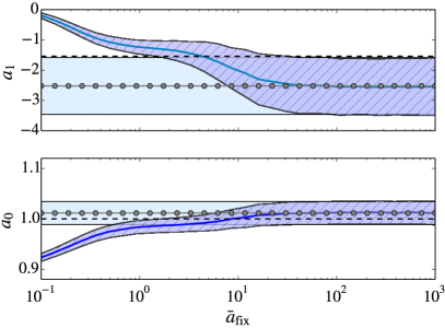
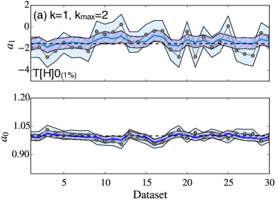
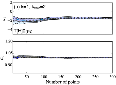
The evidence for different values of is shown in Table 15, and we see that the evidence saturates around , while the ratio of the evidence at to is only about , indicating that no more information is gained for from this data set. Using prior Set C′ with results in excellent agreement of and with their true values, but with not well-constrained. The results for the posterior maxima in the right side of Table 15 confirm the guidance from the evidence that extractions past first order will not contain much information.
In terms of choosing a prior, Fig. 39 demonstrates that at , the first two coefficients are consistent with the true values for between about 2 and 10. We could also compute the posterior to analyze naturalness information contained in the data. Using the simplified prior Set C′ with therefore produces consistent results in this case.
The inclusion of additional information in the parameter estimation is beneficial, as it was in Sec. IV. In this nonlinear problem, the procedure results in the best possible parameter estimates with the available information. Even at overfitting occurs when naturalness information is not included, and the multi-set plot of Fig. LABEL:sub@fig:TH01_datasets_k1_kmax2 shows the benefit of the naturalness prior— and that the consquences of statistical fluctuations are still unavoidable, even with the high-quality data set . The accumulation plot in Fig. LABEL:sub@fig:TH01_accumulated_k1_kmax2 shows that the prior is beneficial even for a large data set until about 10 data sets are available, at which point the uniform prior and naturalness prior results become the same.
The procedures detailed in Fig. 13 are thus directly applicable to parameter estimation in cases when the available data are related nonlinearly to the parameters. We have demonstrated in a simple test case the success of the diagnostics with respect to the type of observable used. Of course, the limitations identified in this section and in the test cases of Sec. IV will still be present in nonlinear applications, but the major theme persists: the best parameter estimates are obtained by using all available information about the problem at hand.
VI Summary and outlook
In this paper, we present a detailed framework for EFT parameter estimation using Bayesian statistics, which naturally combines statistical and systematic uncertainties. Fitting the LECs in an EFT poses a basic dilemma: we want to use more data to suppress the impact of data errors and avoid overfitting, but the accuracy decreases for larger values of the EFT expansion parameters, so using too much can lead to underfitting. By marginalizing over omitted higher-order terms using naturalness priors, we are able to use all of the data, without having to decide a particular value of the EFT parameter at which to break off the fit. In particular, a prior on naturalness suppresses overfitting by limiting how much LECs can play off each other. This in turn means we find stability with respect to expansion order and amount of data.
This success is not achieved automatically, however; there are multiple ways the parameter estimation can go wrong. By studying simple models reflecting the possible behaviors of an EFT, we have identified pitfalls and ways to address them. We have developed a suite of diagnostic tools to guide and analyze the fit of LECs. These diagnostics:
-
•
use the Bayes evidence ratio to find how many LECs can be determined by the data;
-
•
identify potential sensitivity to the choice of prior;
-
•
trace the way the prior eliminates spurious correlations between undetermined coefficients;
-
•
indicate the region in the EFT parameter where a particular LEC is determined;
-
•
show the impact that fluctuations in the data have on the parameter estimation.
They are summarized in Table 2 and a possible flowchart for applying them in parameter estimation is given in Fig. 13. Multiple examples in Sec. III, IV, and V illustrate how to use these tools. These examples are not exhaustive but highlight some important features of Bayesian uncertainty quantification for EFT parameter estimation.
Our goal has been to make this framework adaptable to a wide range of EFT applications. We plan to test the framework in applications such as fitting LECs for the nucleon mass chiral expansion with genuine lattice data and for chiral nucleon-nucleon and three-nucleon forces. This will require us to address practical challenges such as the computational cost of MCMC evaluations, which may require compromises in our procedures. It will also be of interest to investigate whether augmentations of basic least-squares fitting procedures commonly used by practitioners to address the special features of EFTs can be justified within a Bayesian framework.
While we have focused here on parameter estimation, we believe that the Bayesian framework will enable practitioners to consistently achieve all the general goals of UQ for EFT calculations:
-
•
reflect all sources of uncertainty in an EFT prediction using a likelihood or prior for each;
-
•
compare theory predictions and experimental results statistically, with error bands as Bayesian degree-of-belief (DoB) intervals;
-
•
distinguish uncertainties from IR (long-range) vs. UV (short-range) physics by avoiding overfitting;
-
•
provide guidance on how to better extract LECs by exploiting how Bayes’ theorem propagates new info (e.g., will an additional or better measurement or lattice calculation help and by how much?);
-
•
test whether EFT is working as advertised — do our predictions exhibit the anticipated systematic improvement? — by analyzing the trends of DoB intervals and applying model selection.
Investigations are in progress to extend and validate our diagnostics and procedures for each of these goals.
Acknowledgements.
We thank H. Griesshammer, D. Higdon, J. McGovern, E. Lawrence, A. Peter, M. Schindler, A. Steiner, and S. Wild for useful discussions. Useful feedback on the manuscript was provided by A. Dyhdalo, M. Heinz, S. Koenig, S. More, R. Perry, and C. Plumberg. This work was supported in part by the National Science Foundation under Grant No. PHY–1306250, the U.S. Department of Energy under grant DE-FG02-93ER40756, the NUCLEI SciDAC Collaboration under DOE Grant DE-SC0008533, and the Seattle Chapter of the Achievement Rewards for College Scientists Foundation.Appendix A Details on implementation of Markov Chain Monte Carlo via emcee
MCMC sampling methods are particularly suited to efficiently sample pdfs with large parameter spaces Foreman-Mackey et al. (2013), and have been applied widely in many physical applications, such as astrophysics Trotta (2008); Hou et al. (2012). We apply a particular MCMC sampling algorithm called emcee Foreman-Mackey et al. (2013), which is a Python implementation of Goodman and Weare’s affine-invariant ensemble sampler for MCMC. The goal of the algorithm is to improve over traditional Metropolis-Hastings (M-H) methods Metropolis et al. (1953) and modifications that require significant burn-in phases with the price of many computationally expensive evaluations of the pdf. Reference Gelman et al. (2003) contains summaries of several methods for posterior simulation, including the aforementioned M-H methods and Gibbs sampling.
The emcee code uses an ensemble of several walkers to explore the parameter space. Each starts in a user-specified part of the parameter space and is allowed to diffuse, exploring different features of the distribution in parallel. The number of walkers needed to sufficiently explore the parameter space generally depends on the problem of interest, but Ref. Foreman-Mackey et al. (2013) suggests using hundreds of walkers. For the simple model problems in this work we find it is sufficient to use a number of walkers equal to twice the number of parameters, and to be safe we use four times the number of parameters.
The dangers that occur during optimization can also occur with MCMC walkers— they can find unlikely parts of the parameter space and become “stuck”. Assessment of the convergence of the walkers is crucial to diagnose such problems. Sometimes walkers that are not converging can be identified graphically, but several useful quantitative methods exist to diagnose the convergence. Foreman-Mackey et al. advocate using the autocorrelation time, which quantifies the number of evaluations needed to obtain independent samples of the distribution Foreman-Mackey et al. (2013). When the autocorrelation time is large, the number of evaluations needed by the MCMC algorithm to achieve convergence will be large.
They also outline some proxies for assessing convergence Foreman-Mackey et al. (2013). One proxy is the fraction of proposed steps that were accepted in the sampling, called the acceptance fraction , which can be used to diagnose walkers that did not converge during the sampling. We use this simple diagnostic to ensure that walkers converged in our MCMC sampling throughout this work, using the rejection criteria for each separate walker. Low acceptance fractions are a sign that the sampler is stuck in an area of low probability, which often occurs in multimodal distributions. Some methods to deal with multimodality include clustering algorithms Hou et al. (2012) and parallel-tempering ensemble MCMC, which is implemented in emcee.
References
- Kaplan (1995) D. B. Kaplan, (1995), arXiv:nucl-th/9506035 [nucl-th] .
- Phillips (2002) D. R. Phillips, Czech. J. Phys. 52, B49 (2002), arXiv:nucl-th/0203040 [nucl-th] .
- Burgess (2007) C. P. Burgess, Ann. Rev. Nucl. Part. Sci. 57, 329 (2007), hep-th/0701053 .
- Epelbaum (2010) E. Epelbaum, (2010), arXiv:1001.3229 [nucl-th] .
- Descotes-Genon et al. (2004) S. Descotes-Genon, N. H. Fuchs, L. Girlanda, and J. Stern, Eur. Phys. J. C 34, 201 (2004), arXiv:hep-ph/0311120 [hep-ph] .
- Ledwig et al. (2014) T. Ledwig, J. Nieves, A. Pich, E. Ruiz Arriola, and J. Ruiz de Elvira, Phys. Rev. D 90, 114020 (2014), arXiv:1407.3750 [hep-ph] .
- Zhang et al. (2015) X. Zhang, K. M. Nollett, and D. R. Phillips, Phys. Lett. B 751, 535 (2015), arXiv:1507.07239 [nucl-th] .
- Furnstahl et al. (2015a) R. J. Furnstahl, N. Klco, D. R. Phillips, and S. Wesolowski, Phys. Rev. C 92, 024005 (2015a), arXiv:1506.01343 [nucl-th] .
- Pérez and Papenbrock (2015) E. A. C. Pérez and T. Papenbrock, Phys. Rev. C 92, 064309 (2015), arXiv:1510.02401 [nucl-th] .
- Griesshammer et al. (2015) H. W. Griesshammer, J. A. McGovern, and D. R. Phillips, (2015), arXiv:1511.01952 [nucl-th] .
- Furnstahl et al. (2015b) R. J. Furnstahl, D. R. Phillips, and S. Wesolowski, J. Phys. G 42, 034028 (2015b), arXiv:1407.0657 [nucl-th] .
- Navarro Pérez et al. (2013) R. Navarro Pérez, J. E. Amaro, and E. Ruiz Arriola, Phys. Rev. C 88, 024002 (2013), [Erratum: Phys. Rev. C 88, 069902 (2013)], arXiv:1304.0895 [nucl-th] .
- Schindler and Phillips (2009a) M. R. Schindler and D. R. Phillips, Annals Phys. 324, 682 (2009a), arXiv:0808.3643 [hep-ph] .
- Ekström et al. (2013) A. Ekström, G. Baardsen, C. Forssén, G. Hagen, M. Hjorth-Jensen, et al., Phys. Rev. Lett. 110, 192502 (2013), arXiv:1303.4674 [nucl-th] .
- Carlsson et al. (2015) B. Carlsson, A. Ekström, C. Forssén, D. F. Strömberg, O. Lilja, et al., Phys. Rev. X 6, 011019 (2015), arXiv:1506.02466 [nucl-th] .
- Epelbaum et al. (2015) E. Epelbaum, H. Krebs, and U. G. Meißner, Eur. Phys. J. A 51, 53 (2015), arXiv:1412.0142 [nucl-th] .
- Dobaczewski et al. (2014) J. Dobaczewski, W. Nazarewicz, and P.-G. Reinhard, J. Phys. G 41, 074001 (2014), arXiv:1402.4657 [nucl-th] .
- Stump et al. (2001) D. Stump et al., Phys. Rev. D 65, 014012 (2001), arXiv:hep-ph/0101051 [hep-ph] .
- Gregory (2005) P. Gregory, Bayesian Logical Data Analysis for the Physical Sciences (Cambridge University Press, 2005).
- Sivia and Skilling (2006) D. Sivia and J. Skilling, Data Analysis: A Bayesian Tutorial (Oxford University Press, 2006).
- Cox (1946) R. T. Cox, American Journal of Physics 14, 1 (1946).
- Cox (1961) R. T. Cox, The Algebra of Probable Inference (Johns Hopkins University Press, 1961).
- Jaynes (2003) E. T. Jaynes, Probability Theory: The Logic of Science (Cambridge University Press, 2003).
- Jaynes (1957) E. T. Jaynes, Phys. Rev. 106, 620 (1957).
- Foreman-Mackey et al. (2014) D. Foreman-Mackey, A. Price-Whelan, G. Ryan, Emily, M. Smith, K. Barbary, D. W. Hogg, and B. J. Brewer, “corner.py v1.0.0,” (2014).
- Olive et al. (2014) K. Olive et al. (Particle Data Group), Chin. Phys. C 38, 090001 (2014).
- Trotta (2008) R. Trotta, Contemp. Phys. 49, 71 (2008), arXiv:0803.4089 [astro-ph] .
- Epelbaum et al. (2008) E. Epelbaum, H. Krebs, and U.-G. Meissner, Nucl. Phys. A 806, 65 (2008), arXiv:0712.1969 [nucl-th] .
- Foreman-Mackey et al. (2013) D. Foreman-Mackey, D. W. Hogg, D. Lang, and J. Goodman, Publications of the Astronomical Society of the Pacific 125, pp. 306 (2013).
- Lepage et al. (2002) G. Lepage, B. Clark, C. Davies, K. Hornbostel, P. Mackenzie, et al., Nucl. Phys. Proc. Suppl. 106, 12 (2002), arXiv:hep-lat/0110175 [hep-lat] .
- Lepage (1997) G. P. Lepage, (1997), arXiv:nucl-th/9706029 [nucl-th] .
- Griesshammer (2015) H. W. Griesshammer, in 8th International Workshop on Chiral Dynamics (CD 2015) Pisa, Italy, June 29-July 3, 2015 (2015) arXiv:1511.00490 [nucl-th] .
- Griesshammer (2004) H. W. Griesshammer, Nucl. Phys. A 744, 192 (2004), arXiv:nucl-th/0404073 [nucl-th] .
- Bedaque et al. (2003) P. F. Bedaque, G. Rupak, H. W. Griesshammer, and H.-W. Hammer, Nucl. Phys. A 714, 589 (2003), arXiv:nucl-th/0207034 [nucl-th] .
- Higdon et al. (2015) D. Higdon, J. D. McDonnell, N. Schunck, J. Sarich, and S. M. Wild, J. Phys. G 42, 034009 (2015), arXiv:1407.3017 [physics.data-an] .
- Bernard (2015) C. Bernard, in 8th International Workshop on Chiral Dynamics (CD 2015) Pisa, Italy, June 29-July 3, 2015 (2015) arXiv:1510.02180 [hep-ph] .
- Bali et al. (2013) G. Bali et al., Nuclear Physics B 866, 1 (2013).
- Schindler and Phillips (2009b) M. R. Schindler and D. R. Phillips, Annals Phys. 324, 2051 (2009b).
- Hou et al. (2012) F. Hou, J. Goodman, D. W. Hogg, J. Weare, and C. Schwab, Astrophys. J. 745, 198 (2012), arXiv:1104.2612 [astro-ph.IM] .
- Metropolis et al. (1953) N. Metropolis, A. W. Rosenbluth, M. N. Rosenbluth, A. H. Teller, and E. Teller, Journal of Chemical Physics 21, 1087 (1953).
- Gelman et al. (2003) A. Gelman, J. B. Carlin, H. S. Stern, and D. B. Rubin, Bayesian Data Analysis (Chapman and Hall/CRC, 2003).