The Omega-Infinity Limit of Single Spikes
Abstract
A new infinite-size limit of strings in is presented. The limit is obtained from single spike strings by letting the angular velocity parameter become infinite. We derive the energy-momenta relation of single spikes as their linear velocity and their angular momentum . Generally, the , limit of single spikes is singular and has to be excluded from the spectrum and be studied separately. We discover that the dispersion relation of omega-infinity single spikes contains logarithms in the limit . This result is somewhat surprising, since the logarithmic behavior in the string spectra is typically associated with their motion in non-compact spaces such as AdS. Omega-infinity single spikes seem to completely cover the surface of the 2-sphere they occupy, so that they may essentially be viewed as some sort of ”brany strings”. A proof of the sphere-filling property of omega-infinity single spikes is given in the appendix.
1 Introduction and Motivation
The AdS/CFT correspondence has been revolutionized during the past ten years by the introduction of integrability methods [1, 2] that can be used in order to solve the theories on both sides of the correspondence.222In the large-/planar limit (), the string theory is essentially free () for . AdS5/CFT4 is also thought to be quantum integrable in the planar limit. As far as a certain class of (long) rotating strings is concerned however,333These are dual to long operators of super Yang-Mills (SYM) at strong ’t Hooft coupling . integrability tools and techniques (such as the ABA, TBA, Y-system, QSC, etc.) have neither been sufficiently developed, nor do they provide the high-loop spectroscopic predictions that they typically yield at either weak coupling (e.g. 9-loop Konishi, [3]) or at strong coupling and small spins (e.g. 3-loop Konishi [4]).444Even the more recently developed techniques, such as the quantum spectral curve method [5], succeed only when the coupling is weak and at strong coupling when the spin is small. In this paper we will be dealing with the spectral problem in precisely one of those regimes (namely long strings in ) where the existing spectroscopic machinery is still too complicated to be used for explicit calculations of operator scaling dimensions and string-state energies.
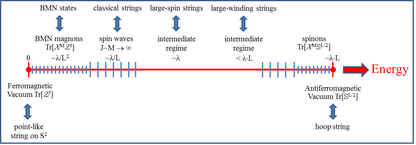
A general description of the spectrum of planar AdS/CFT, based on the structure of the Heisenberg ferromagnet, can be found in the references [7] and [8] (see also figure 1). Let denote the scaling dimension and the length of the operator.555In the following, will denote the three complex scalar fields of SYM, composed out of the theory’s six real scalars . It was proven in [9] that the one-loop dilatation operator of the sector of the theory (consisting of all the single-trace operators ) is given by the Hamiltonian of the ferromagnetic XXX1/2 Heisenberg spin chain. We consider the thermodynamic limit . Qualitatively the spectrum is expected to be the same for greater values of the ’t Hooft coupling . For the strongly coupled description of AdS/CFT, the generic structure of the string spectrum is also expected to be the same. The spectrum will also be similar in all the other sectors of AdS/CFT.
The bottom of the spectrum is occupied by the BPS operator Tr that is the vacuum state of a ferromagnetic spin chain with energy . The vacuum is dual to a point-like string that rotates at the equator of S. Magnons are excitations above the ferromagnetic vacuum with energies and large spins, . An -magnon operator Tr () is dual to a nearly point-like (BMN) string that rotates in with two angular momenta and (finite).666To get a BMN string [10] one more condition is needed, namely that the ratio must be held fixed. For , we obtain a low-energy spin wave with . At the intermediate regime we find states with . The latter are dual to long strings that rotate on the 2-sphere, e.g. GKP strings [11], giant magnons [12], etc.
The spectrum terminates at the antiferromagnetic (AF) vacuum Tr, where are spin-neutral composites of the fields of SYM. The AF vacuum has [13] and it is dual to the so-called ”hoop” string, a circular stationary string of infinite length that is wound around the equator of S2 [8]. Spinons Tr, are excitations of the AF state with energies . Of course we have mostly described what happens in the sector, however one may generalize this discussion to the entire AdS/CFT, by replacing the scalar impurity with any of the fields of SYM, and move from to the full AdS spacetime in order to get the dual picture.
The energy of single magnon states Tr in a spin chain of total length is [14]:
where is the magnon’s quantized momentum. This formula can also be derived if one extends the corresponding symmetry algebra by two central charges [15]. Extending the symmetry algebra is necessary in order to obtain magnon states with non-vanishing total momentum and violate the cyclicity of the trace condition. For this reason one-magnon operators with non-vanishing momentum are usually written as states rather than single-trace operators:
(1) is only valid asymptotically, namely up to a gauge theory loop-order that is less than the length of the spin chain. When the size of the spin chain becomes infinite (), (1) holds to all loops from weak to strong coupling. In this case we may expand (1) at both small and large coupling :
Now it was shown by Hofman and Maldacena in [12] that it is possible to obtain the string theory duals of magnons in the intermediate energy regime (1) (where ), by considering a different kind of limit than the BMN. Giant magnons (GM) are classical open strings with a single spin that rotate in . They can be identified with the string theory duals of magnons, because their energy-spin relation at tree level
is identical with the corresponding term in the strong coupling expansion (1) of (1). The same is true for the S-matrix of giant magnons, which can be shown to reproduce the result from the gauge theory side. The corresponding infinite-volume one-loop shifts have also been found to agree [16, 17].
When the size of the system becomes finite, (1) is no longer valid to all loops but there exists a critical loop-order (equal to the length of the operator) above which (1) starts receiving finite-size or wrapping corrections. If the string theory description of strongly coupled SYM is correct, we should expect to find these finite-size corrections encoded in the perturbative string expansion even at tree level. Finite-size giant magnons were introduced in [18, 19]. A study of their classical finite-size corrections can be found in [20].888See also the thesis [21] and the talk [22].
The direct analogs of giant magnons for the AF ground state are single spikes (SSs) [23, 24]. These are the string theory duals of SYM (single) spinon states [25],
which are elementary excitations above the AF vacuum state Tr [8]. Finite-size single spikes are open single spin strings that rotate in and are described in terms of their linear velocity and the angular velocity :999The term ”angular velocity” is actually a misnomer for the parameter , since the true angular velocity of the string is given by , where is a function of the string variables and . The authors kindly apologise to the reader for taking the permission to conventionally call the parameter angular velocity.
The former regime is known as the elementary region and the latter as the doubled region of single spikes. Like giant magnons, single spikes also belong to the class of long strings/strongly coupled operators for which there are no advanced spectroscopic tools at our disposal. Single spikes can be transformed to giant magnons by means of the transform or ”2D duality” [25]:
In fact, (1) maps the elementary region of single spikes to the elementary region of giant magnons and the doubled region of single spikes to the doubled region of giant magnons. In [20], two more symmetries between the equations of motion of giant magnons and single spikes were found.101010Namely the and the transforms, where is given by equations (2.1)–(2.2). These either transform between the elementary regions of GMs and SSs, or map their elementary regions to their doubled regions. For more, refer to the appendix A.5 of [20].
The dispersion relation of single spikes provides their conserved energy in terms of their other conserved charges, i.e. their linear momentum and their angular momentum . For , the energy and the linear momentum become infinite and single spikes have infinite length and winding (since their length/winding is proportional to their linear momentum). However the difference of the two (scaled) charges is finite:
For the single spike reduces to the infinitely wound hoop string that is dual to the antiferromagnetic ground state Tr of SYM and has the following dispersion relation:
When , single spikes have finite but still large size/winding111111As a reminder, a string of infinite size is defined as having infinite worldsheet size and therefore infinite energy (c.f. equation (2.1) below). Infinite momentum implies that the angular extent of the string (or its winding in units of ) is also infinite (c.f. equation (2) below). In our manuscript ”string length” is an alias for ”string winding”, or the length of the string in the target space. The size (i.e. the energy) of single spike strings is large/infinite because their energy is equal to their momentum (i.e. their length/winding/angular extent) to lowest order (c.f. equation (1)) and the latter is also large/infinite. That is why the terms infinite size/winding are used interchangeably throughout our paper. and their dispersion relation assumes the following general form [20] (at strong coupling, ):
where are some trigonometric coefficients and
In the elementary region (), the first few terms of (1) are:
while in the doubled region (), the corresponding coefficients are given by:
More terms can be found in appendix B of the paper [20]. For the code that generates these expansions, the reader may refer to the thesis [21]. The above results are in complete agreement with the infinite-size/winding limit (1) that we saw above. Just note that if we set , the momentum becomes infinite () and all the exponentials in (1), (1) and (1) vanish. (1) also agrees with the leading finite-size correction computed by Ahn and Bozhilov in [26].
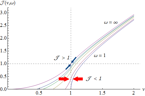
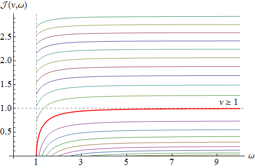
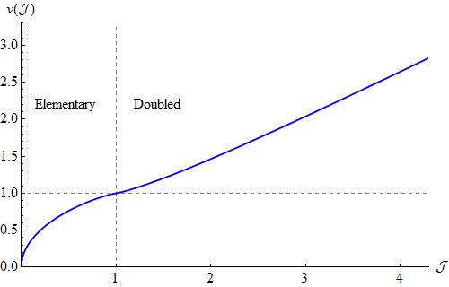
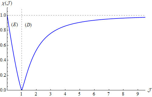
In the limit , it seems that the exponential suppression drops out of (1) since . A closer look at the expansions (1)–(1) reveals that many of the trigonometric coefficients blow up in the limit , signaling that the value (in the large-winding region ) is probably singular and has to be treated separately. Furthermore, for it is possible that the spin approaches unity from above (—see figure 3) and essentially becomes complex. Indeed, it was proven in [20] that the algorithm leading to (1)–(1) is dysfunctional for , , and it cannot be used.
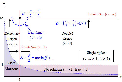
The aim of the present paper is to clarify the above situation by computing the dispersion relation of classical single spikes in the infinite-size/winding limit (see figure 2):
where (1) is no longer valid.
To get going, let us first note that the limit of single spikes is an infinite-size/momentum limit, that is
a fact already anticipated in [20]. The dispersion relation of single spikes in the limit becomes:
where is a function of the (scaled) angular momentum that depends on the region (elementary/doubled) of single spikes that we are considering. In figure 3, corresponds to the purple line that passes through the point . Interestingly, (1) agrees with (1) in the double infinite-size/winding limit , :
As we have already said, we have computed (1) in the region (1) of single spikes. If we define,
where the upper signs refer to the elementary region and the lower signs to the doubled region of single spikes, then the general form of in the region (1) is the following:
where the ’s are given by
The proof of the dispersion relation (1), along with the computation of some of the coefficients in both the elementary and the doubled region are the main results of our paper. The structure of (1) for infinite size/winding single spikes is highly reminiscent of the large-spin expansions of the anomalous dimensions of twist-2 operators and those of Gubser-Klebanov-Polyakov (GKP) strings in AdS3 [27]. However, the leading logarithm , as well as all the leading terms that were present in the dispersion relation of twist-2 operators and GKP strings, are missing from (1). Yet another difference is that the coefficients of (1) depend explicitly on the spin .
Our paper is organized as follows. In §2 we briefly revisit the definition of finite-size single spikes. In §3 we study the dispersion relation of single spikes in the limit , in both the elementary and the doubled region. We discuss our results in §4. In appendix A we establish the consistency of the limit of single spikes by explicitly deriving the corresponding string sigma model solutions and conserved charges. We also provide a proof of the space-filling property of omega-infinity single spikes.
2 Finite-Size Single Spikes
As we have already mentioned, single spikes are open single spin strings that rotate inside the subset . Let us see how they can be obtained from the generic configuration of open (bosonic) strings in :
In this paper we work with the following parametrization of AdS:
and set
In the above parametrization, the string’s embedding coordinates become:
while the conformal () string Polyakov action is given by
In the static time gauge () the corresponding Virasoro constraints and Pohlmeyer reduction become:
where the Pohlmeyer field satisfies the following sine-Gordon (sG) equation:
To obtain single spikes we insert the ansatz
into the Virasoro constraints and the Pohlmeyer reduction (2)–(2) and impose the b.c.’s
where are the string’s world-sheet endpoints () and the string’s constant angular extent equals its conserved linear momentum. Equations (2)–(2) become:
| Doubled Giant Magnon | Elementary Giant Magnon | – | |
| \cdashline1-4 | – | Elementary Single Spike | Doubled Single Spike |
If , the system (2)–(2) affords a solution only for and . Actually there only exist two solutions, namely the point-like string () that rotates around the equator of the 2-sphere and its dual under the transform (1) hoop string () that is infinitely wrapped around the equator of the 2-sphere and remains at rest.
One may prove that the constraint equations (2)–(2) are compatible with the equations of motion that are derived from the action (2), while satisfies the sG equation (2). Dividing the square root of (2) with (2), we obtain:
All in all, there exist four different solutions of (2)–(2), depending on the relative values of the string’s linear velocity and angular velocity . These are the following (see table 1):
Below we shall focus on the single spike regions (3) and (4), for which and respectively. More can be found in appendix A of the paper [20].
2.1 Single Spikes: Elementary Region
In the elementary region of single spikes,
we set:
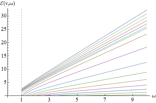
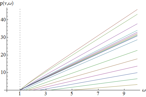
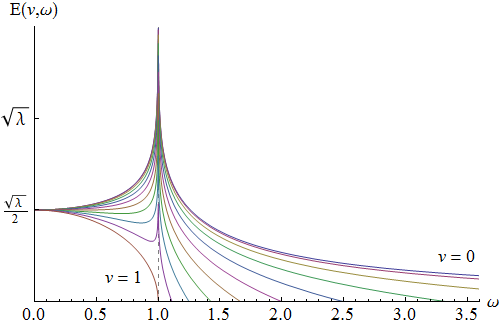
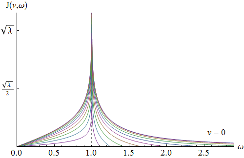
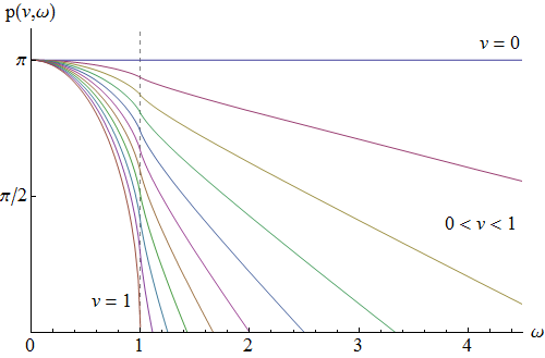
The conserved energy and momenta (angular and linear) of single spikes in the elementary region are given by:131313To obtain the charges of (elementary/doubled) single spikes we must compute , from (2)–(2) and from (2):
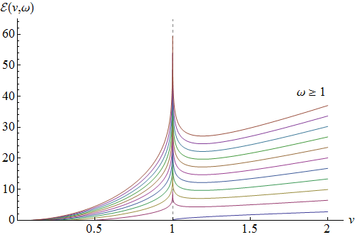
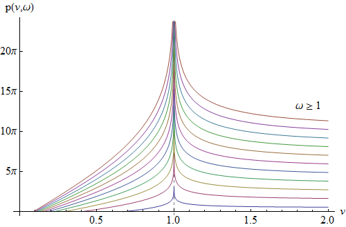
We have plotted (2.1)–(2.1) in terms of the linear velocity and the angular velocity in figures 5 and 6 respectively. The system of equations (2)–(2) admits the following solution:
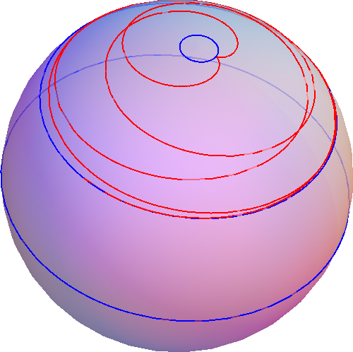
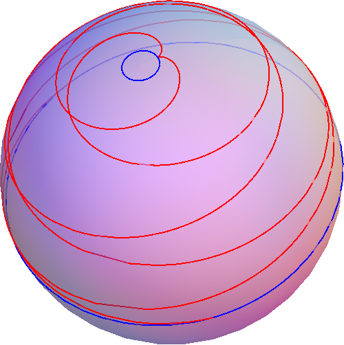
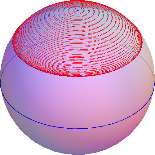
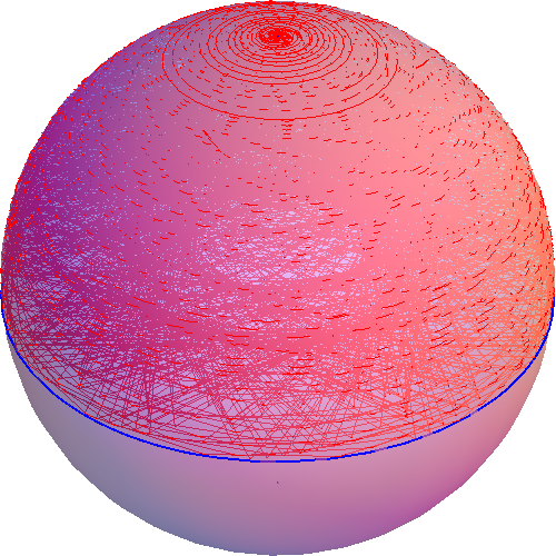
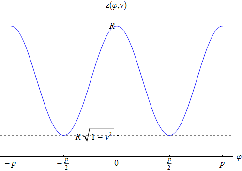
Elementary single spikes may be visualized by plotting equation (2.1) on a sphere with . We obtain the moving string on the left-hand side of figure 4.
2.2 Single Spikes: Doubled Region
Single spikes in the doubled region have
and again we define
The conserved energy and momenta (angular/linear) of the doubled single spike are given by:
The plots of (2.2)–(2.2) in terms of the velocities and can be found in figures 5 and 6. The system of equations (2)–(2) admits the following solution in the region (2.2):
The doubled single spike has been plotted on the right-hand side of figure 4. The open string gradually unwinds from the north pole and starts winding around the south pole. Then the motion repeats itself.
2.3 Infinite-Size Limit
In the limit , the energy and the linear momentum of both the elementary and the doubled-region single spikes become infinite. Let us briefly review this limiting case before proceeding to examine yet another infinite-size limit of single spikes. For , the single spike ansatz (2)–(2) becomes:
The corresponding charges can be easily computed, giving rise to the dispersion relation (1):
The solution to the equations of motion (2)–(2) is:
3 The Limit of Single Spikes
We are now ready to explore the limit of single spikes. Let us first prove that the limit of the ansatz (2)–(2), in the single spike region (, ), is an infinite-size limit.
3.1 Elementary Region
We begin with the single spike elementary region for which . For the conserved charges (2.1), (2.1), (2.1) of the elementary single spike become:
Clearly when . Therefore in the limit , the system’s size and its momentum/winding become infinite. See also the plots in figure 7.
The dispersion relation of single spikes in the elementary region is the following:
where gives the string’s velocity in terms of its spin. It can be found by inverting (3.1):
For , the elliptic integrals do not contain a logarithmic singularity and (3.1) may easily be inverted with . The first few terms of the result are:
For , we may invert (3.1) by using the series inversion technique that was employed for GKP strings in AdS3 in reference [27]. See also appendix B. The result is:
where and is given by:
The argument of the W-function is in the branch. The branch is the only real branch of the function where . We may expand the W-function by using its Taylor expansion (D) around the point . We find,
in full agreement with the inverse spin function (C.2.1) that we have computed in appendix C.2 with . We find the appearance of logarithms in the dispersion relation of strings in rather surprising. Usually, the emergence of logarithms in the dispersion relations of single-trace operators of SYM is associated with the presence of covariant derivatives inside the operators. Their dual strings then acquire a spin component inside the non-compact AdS space. As we have also mentioned in the introduction, the inverse spin function of single spikes that we find looks very much like the dispersion relation of twist-2 operators Tr and the one of their dual closed folded GKP strings in AdS3. However, the characteristic leading logarithm of twist-2 operators is missing from and the coefficients of each term depend explicitly on the scaled spin variable . Yet another difference that could help justify the presence of logarithms in (3.1), is that the spin variable is equal to the logarithm of the real spin , so that we essentially have reciprocals of logarithms and logarithms of logarithms inside the expression of that we must then subtract from unity and take the square root in order to obtain the corresponding dispersion relation.
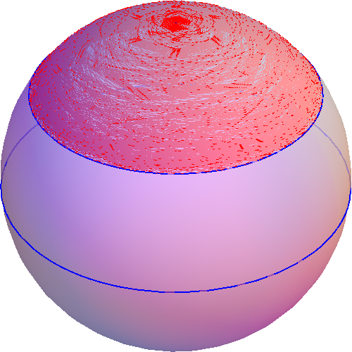
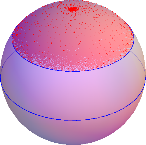
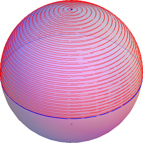
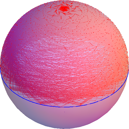
In figure 7 we have plotted some elementary single spikes for increasing values of the angular velocity . The open strings seem to gradually take over all of the space on the 2-sphere between the parallel (that binds their motion from below) and the pole, so that they eventually (as ) resemble a 2-dimensional brane rather than a string. These ”brany strings” are of course very reminiscent of the ”stringy branes” that were introduced in [28], i.e. M2-branes inside 11-dimensional AdS/CFT spacetimes that have only one stringy mode instead of multiple ones and share the same dispersion relation with strings that live inside 10-dimensional AdS/CFT spacetimes. Of course, we obtain exactly the same graphs by plotting the omega-infinity limits (A.1)–(A.1) of the solutions (2.1)–(2.1). These have been derived in appendix A. The sphere-filling property of omega-infinity (elementary) single spikes is proven in appendix A.3.
3.2 Doubled Region
In the doubled region () the conserved charges (2.2), (2.2), (2.2) of the single spike become, for :
Again when , and the limit is an infinite-size/momentum/winding limit. Some plots of doubled single spikes with can be seen in figure 8.
The dispersion relation of single spikes in the doubled region is the following:
where gives the single spike’s velocity in terms of its spin. To find it we must invert (3.2):
In the limit the inversion of (3.2) with is rather straightforward. We find,
For we may invert (3.1) by the method of reference [27] (see also appendix B). The result is:
This time while is given by:
The argument of the W-function is in the branch. We must choose the branch of the W-function, since it is its only real branch where the that we find has the desired behavior (and therefore ). Again we may expand the W-function by using its Taylor expansion (D) around the point . Then,
(3.2) fully agrees with the inverse spin function (C.2.2) that was computed in appendix C.2 with . Once more we note the appearance of logarithms in the dispersion relation. In figure 8 we have plotted some doubled single spikes for increasing values of the angular velocity . Exactly the same graphs could have been obtained if we had plotted the omega-infinity limits (A.2)–(A.2) of the corresponding solutions (2.2)–(2.2). See appendix A.3 for a proof of the sphere-filling property of doubled single spikes in the omega-infinity limit.
3.3 General Form of the Dispersion Relation for
We are now in a position to write down a general formula for the dispersion relation of single spikes (both elementary and doubled) in the limit . The dispersion relation is:
If we define
then the inverse spin function has the following general form:
where the ’s are given by
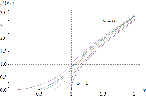
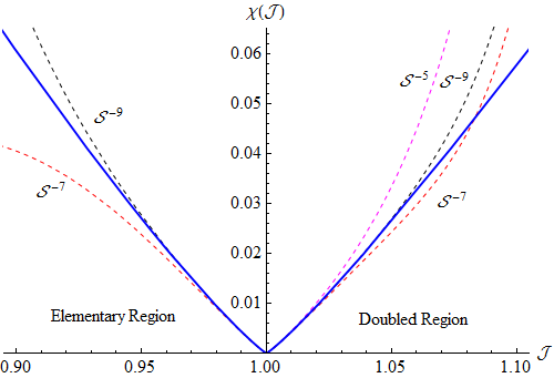
The values of the coefficients (in the elementary and doubled regions respectively) can be read-off from (3.1)–(3.2). In figure 9 we have plotted the spin function parametrically, based on (3.1)–(3.2) (the precise form is given in equation (B) of appendix B). The dotted lines correspond to the approximation (3.3), up to and including the , and terms.
4 Discussion
4.1 Single Spike Dispersion Relations
Let us summarize what we learned about the dispersion relations of classical single spike strings. The size/momentum/winding of elementary and doubled single spikes becomes infinite in two different limits (see figures 2–3). The limit [23, 24] (see §2.3) in which:
and the limit that we studied in §3 of the present paper:
where is found by inverting the spin function
For , the size/momentum/winding of single spikes is no longer infinite but is still quite large and the dispersion relation (4.1) receives exponentially suppressed finite-size corrections that have the following general form (at strong coupling, ) [20]:
where are trigonometric coefficients (see (1)–(1)) and we have defined:
As long as the exponential suppression factor for , the dispersion relation (4.1) is perfectly well-defined and fully convergent. However it seems that when , becomes finite and the exponential suppression disappears from (4.1). In fact (4.1) clearly diverges if we first consider the limit and then the limit . Note also that many of the trigonometric coefficients of (4.1) (cf. (1)–(1)) blow up for , implying that the value of the angular momentum is probably singular. For , it is also possible for to approach unity from above (—see figure 3), rendering in (4.1) a complex number.
In appendix C of the paper [20] it was argued that the dispersion relation (4.1) is valid only in the following regime:
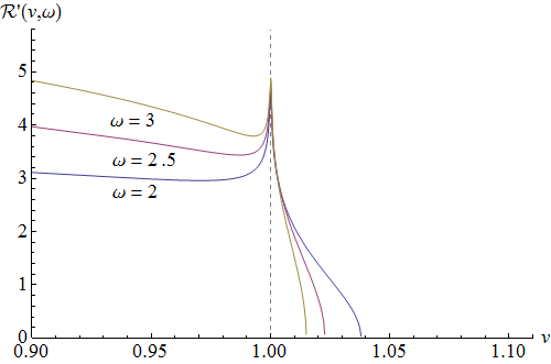
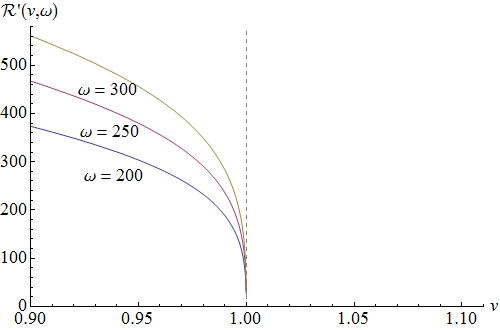
The reasoning was quite simple: if is finite, then the inverse momentum function (defined in (4.3) below) that is used in order to obtain (4.1) does not have the correct behavior as . As a matter of fact we may show that (4.1) becomes less valid as the angular velocity increases towards infinity. Let us define as:
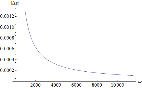
i.e. gives the behavior of the coefficient in the large winding regime () where the momentum becomes infinite. In figure 10 we have plotted near for various values of the angular velocity . There is a delta function peak at but, as we leave the vicinity of this point, may become finite and (4.1) then is ill-defined and divergent.
In total there are three paths away from the point (see figure 3): (a) For and the dispersion relation of infinite-size/winding single spikes is (4.1) which is well-defined and convergent. (b) For and , in (4.1) becomes finite and consequently (4.1) and (4.1) no longer hold. In this case (4.1) is valid and we have shown in §3.3 that the inverse spin function of single spikes is given by:
where
and we have defined
Of course, (4.1) and (4.1) agree with each other in the double infinite-size/momentum/winding limit :
(c) Finally, for , the dispersion relation (4.1) will receive finite-size corrections and its regime of validity is expected to overlap with that of (4.1) in certain regions. However there should exist regions where only one of them will be valid.
4.2 Infinite-Size Limits in
Here’s a short summary of infinitely sized strings in . Giant magnons acquire infinite size when the angular velocity parameter becomes unity. Single spikes on the other hand become infinitely sized either if their linear velocity becomes unity or if the angular velocity parameter becomes infinite as we have shown in this paper.
All of these infinite-size limits appear in both the elementary and the doubled regions of giant magnons and single spikes. Now it is obvious from the plots of the charges of giant magnons in figure 11 that is the only infinite-size limit of giant magnons. The corresponding plots of single spikes in figure 5 however imply the existence of an additional infinite-size limit for them, obtained whenever their velocity becomes infinite in the doubled region ().
In the limit, and the charges of doubled single spikes become:
Therefore the size and the angular momentum of single spikes become infinite for , whereas their momentum/winding remains a constant. The corresponding dispersion relation is rather simple in this case:
4.3 Other Topics
To avoid possible ambiguities with the limiting procedure , let us give a formal definition of the omega-infinity limit of single spikes. Consider an ordinary single spike with finite values of and . Then gradually start increasing . The worldsheet size and the physical length of the string will also increase. We identify an omega-infinity single spike with the ideal configuration that results when the size and length of the above string become infinite for and .
The resemblance of (3.3) to the generic dispersion relation of twist-2 operators and GKP strings in AdS, that is known to possess the property of reciprocity, makes us want to check whether (3.3) also has this remarkable property. By reciprocity we mean that the series
of inverse anomalous dimensions contains only even powers of the spin variable and it is symmetric under the transformation . For twist-2 operators and GKP strings, this symmetry leads to a set of relations between the coefficients that are known as MVV (Moch-Vermaseren-Vogt) relations. We have explicitly checked (3.1)–(3.2) for reciprocity and we have found that none of the odd-powered coefficients in the corresponding formulae (4.3) vanishes. We therefore conclude that the dispersion relation (3.3) of single spike strings in the omega-infinity limit, does not have the property of reciprocity.
Being located near the top of the AdS/CFT spectrum, single spike strings are expected to be unstable. The vacuum (i.e. the hoop string) is also unstable as it can roll towards either pole to a configuration of lower energy. The instability of the hoop string and the single spike (elementary/doubled) is most easily proven by using their Pohlmeyer images in the sine-Gordon equation. They correspond to spectrally unstable superluminal () rotational/vibrational wave solutions of sG. They may be stabilized however, either by adding more spins [29], or by turning on appropriate flux terms, or generally by introducing any kind of forcing that could result in a set-up similar to Kapitza’s pendulum. In the case of omega-infinity single spikes, we may create a stable closed IIB string in by adding a stabilizing counterpart along the opposite hemisphere.
In appendix A.3 we have provided a proof of the sphere-filling property of omega-infinity single spikes. An interesting relevant open question is whether the omega-infinity limit of single spikes can be further shown to satisfy an equation of relativistic membranes on some appropriately chosen spacetime. From the point of view of the Pohlmeyer reduction it would be especially intriguing to know what the reduction of a dimensional surface really looks like, even in the very special case of a brane that is made up from just one very long string. The quantization of these configurations could also lead to very useful conclusions about their true nature, be it stringy or brany.
Finally, a more or less standard exercise in the context of the present paper, would be to compute the finite-size corrections that are relevant to the limit of single spikes. The corresponding inverse spin function has the following form:
where, in the elementary region ()
and, in order to comply with the notation of [20],
The first few terms of in the elementary region are the following:
with running in even negative powers. From (4.3), we may compute the first few large- corrections to :
which are obviously of the form (4.3). The corresponding infinite-size coefficients for , can be found in appendix C.2.
To obtain the large- corrections to the energy of (elementary) single spikes, we must plug the inverse spin function (4.3) into the corresponding expression of the energy (2.1). We find:
A simple computation shows that (4.3) is fully consistent with the infinite-size dispersion relation (1)–(3.1). Apparently, the finite-size corrections of the energy run in odd (negative) powers of . In the doubled region the results should be similar. Of course, the full-fledged computation of large-omega corrections (in both the elementary and the doubled regions) constitutes a subject matter all by itself. We therefore postpone it for a future publication.
5 Acknowledgements
The authors are thankful to an anonymous referee of Nuclear Physics B that brought the issue of convergence of formulas (1)–(1) to their attention during the peer-reviewing process of the paper [20]. We would like to thank Marius de Leeuw, Benjo Fraser, George Georgiou, Jens Hoppe, Mariusz Hynek, Holger Bech Nielsen, Nikolaos Tetradis and Matthias Wilhelm for illuminating discussions. E.F. acknowledges Luis Álvarez-Gaumé for instructive discussions and generous support. G.L. is grateful to Charlotte Kristjansen and the Niels Bohr Institute for hospitality and support while this work was in progress, and to Jens Hoppe and the KTH Royal Institute of Technology for hospitality and support during the completion of this work.
The research of E.F. has been partially supported by the ”ARISTEIA” action (Code no.1612, D.654) and title ”Holographic Hydrodynamics” of the ”operational programme education and lifelong learning” and is co-funded by the European Social Fund (ESF) and National Resources. The research of M.A. and G.L. at N.C.S.R. ”Demokritos” is supported by the General Secretariat for Research and Technology of Greece and from the European Regional Development Fund MIS-448332-ORASY (NSRF 2007–13 ACTION, KRIPIS).
Appendix A Solutions & Charges in the Limit
In the present appendix we will derive the solutions of the Virasoro constraints/equations of motion, along with the conserved charges of single spikes. Let us first write down the limit of the Virasoro constraints (2)–(2) and the Pohlmeyer reduction (2):
We are also going to use the following equations:
in the omega-infinity limit. Notice that although for , this factor has explicitly been included in the above equations. The reason is quite subtle. Even though for the Virasoro constraint (A), we want to integrate this equation in which case we must take into account the fact that the integrating variable can become infinite.141414 takes values between , where is the string’s worldsheet size (A.1)–(A.2) (equal to in the omega-infinity limit) and takes values between . Therefore takes values between for single spikes. This makes finite and not equal to zero as one could assume by naively taking in (A).
The same is true for the conserved charges of single spikes. The factors have to be retained, either because the charge eventually becomes infinite in the limit or because the corresponding zero/pole cancels and the charge is finite and non-zero. With these considerations in mind we find the following results.
A.1 Elementary Region ()
The conserved charges become, for :
Note that we retrieve the dispersion relation (without the that is subleading with respect to ). The solutions of the equations of motion are:
where . The plots of single spikes in the limit coincide with the ones that have been drawn in figure 7. The corresponding Pohlmeyer reduction is:
A.2 Doubled Region ()
The conserved charges become, for :
Again, the dispersion relation does not contain the subleading contribution . The equations of motion (A)–(A) are solved by:
with . Plots of single spikes in the limit can be found in figure 8. The Pohlmeyer reduction of single spikes in the doubled region reads:
A.3 Proof of the Sphere-Filling Property
We may use the solutions (A.1)–(A.1)/(A.2)–(A.2) of the (elementary/doubled) single spike Virasoro constraints in the limit in order to prove that they will eventually become 2-dimensional by completely covering the surface of the 2-sphere between their lowest points and the pole. To this end let us first express the variable given by (A.1)–(A.2) (in the limit ) in terms of the angle in (A.1)–(A.2):
has been plotted on the left of figure 12. It is a periodic function (of period ) that oscillates between the parallel and the pole . To prove that the string will cover the surface of the 2-sphere in the omega-infinity limit, we need to show that the distance between two adjacent string windings approaches zero as . After exactly one winding around the sphere, becomes . We may plot the function for increasing angular velocities at the point where it attains its maximum value, namely . The result in both single spike regions (elementary/doubled) is shown on the right of figure 12. The same conclusion can be reached if we expand (A.3) around :
To complete the proof, note from (A.1)–(A.2) that , so that constant. On the other hand, . Thus two neighboring string orbits come arbitrarily close to each other in the limit and the string becomes a sphere-filling curve.
Appendix B Inverse Spin
This appendix deals with the calculation of the dispersion relation of single spikes in the infinite-size limit , for . As we have explained in §3, the energy of single spikes for is given by
where is the expression for the velocity of the single spike in terms of its spin, found by inverting
in terms of the velocity . In the following we are going to show explicitly how (B) can be inverted for . Let us first express (B) in terms of the more convenient variables and :
In figure 13, we have plotted the inverse (spin) functions of (B)–(B). For simplicity, both variables and of (B) will henceforth be denoted with .
For , (B) can be expanded in a series by using the formulas (E)–(E) of appendix E:
In the elementary region, the coefficients and are given by:
are known as harmonic numbers. In the doubled region, the coefficients and are given by:
where,
Note that as , with the minus sign corresponding to the elementary region and the plus sign to the doubled region of single spikes (cf. figure 13). The procedure with which (B) can be inverted has been laid down in the paper [27]. We repeat it here for convenience. First, we solve (B) in terms of the logarithm:
Secondly we perform all the products and exponentiate the result. This leads us to the following series
for the inverse spin function in the elementary region (). In the doubled region, the corresponding series becomes (reverting again to the notation ):
Both series (B)–(B) have the following general form:
where the ’s are linear functions of the (scaled) angular momentum . (B) is the same as equation of the paper [27]. It can be inverted in precisely the same way. Let us repeat the steps here. First, we define the variable as follows:
where is the Lambert W-function (see appendix D) and as . (B) gives the leading-order solution of (B). From the two real branches of the W-function we have to select the branch (cf. figure 14) for which and .151515Had we chosen the branch, we would have and , which is inconsistent with the limit that we are examining. Further, we set:
getting the following equation for the variable :
This series may be inverted in terms of the variable and the result may then be plugged into (B), giving:
where,
Plugging the values of the coefficients (as given by (B)–(B)) in each of the two regions (the elementary and the doubled) into equation (B), we are led to the expressions (3.1)–(3.2) that give the inverse spin function of single spike strings with , in the limit .
Appendix C Numerics
In this appendix we are going to use in order to compute the inverse spin function of single spikes, in the limit . As we have proven in §3.1–§3.2, the dispersion relation of single spikes is:
The inverse spin function is found by inverting the expressions (3.1)–(3.2) for the angular momentum . As we have shown in appendix B, both can essentially be brought to the following form:
where for the elementary region and for the doubled region. The coefficients and for each of the two regions have been written down in (B)–(B).
The method of the paper [27], with which the series (C) can be analytically inverted, has been reviewed in appendix B. The final results (3.1)–(3.2) can be expressed in terms of the Lambert W-function in its branch. In the present appendix we provide the computer code with which the inverse spin function can be numerically computed with and present the results of the calculations which allow us to directly verify our analytic expressions (3.1)–(3.2).
C.1 Algorithms
In order to invert equation (C) numerically, we must first cast it in the appropriate form [21]. Solving for the logarithm we obtain:
as we did in (B) above.
C.1.1 Elementary Region
We now make the following change of variables in (C.1):
getting,
If we invert this equation for , the variable can be obtained from equation (C.1.1). Here’s the code (to run it, just copy-paste it in a notebook):
c[n_]:=1/(4n)((2n-3)!!/(2n-2)!!)^2;cc[0]:=0;b[0]:=1;b[n_]:=-4c[n](Log[2]+HarmonicNumber[n]-HarmonicNumber[2n]+(2n+1)/(4n(2n-1)));y[m_,S_,J_,u_]:=Series[u+2Log[2]-S-(J-Sum[(b[n]((4(1-J)/S)Exp[u])^n),{n,0,m}]) *(Sum[(c[k]((4(1-J)/S)Exp[u])^k),{k,1,m}])^-1,{u,0,m}];\[Chi][m_,S_,J_,v_]:=Series[Normal[Series[Normal[(4(1-J))/S *Exp[InverseSeries[y[m,S,J,u],v]]],{J,1,m}]],{S,\[Infinity],m}];nn=5;\[Chi][nn,S,J,v];Collect[%/.{v->Log[S],J->1-L},{S,Log[S],Log[2]},FullSimplify]
Let us briefly explain what the above code does. and are just the series coefficients , of the elementary region that were given in (B)–(B). Series stands for equation (C.1.1) and gives (C.1.1). The code inverts (C.1.1) for , then plugs the result in (C.1.1) and expands the resulting series around and . The final output is generated from the last three lines. Instead of , the variable is used. For terms, the program takes about s to run in our system.
C.1.2 Doubled Region
In the doubled region, we make the following change of variables in equation (C.1):
so that (C.1) becomes:
Once again, the code consists in inverting (C.1.2) for and then plugging the result in (C.1.2) in order to obtain the inverse spin function (the code can be directly copy-pasted and run in ):
d[n_]:=-(1/2)((2n-1)!!/(2n)!!)^2;h[n_]:=-4d[n]*(Log[2]+HarmonicNumber[n]-HarmonicNumber[2n]);f[n_]:=-(d[n]/(2n-1));g[n_]:=-4f[n]*(Log[2]+HarmonicNumber[n]-HarmonicNumber[2n]+1/(2(2n-1)));c[n_]:=Sum[((2k-1)!!/(2k)!!)(d[n-k]-f[n-k]),{k,0,n}];b[n_]:=Sum[((2k-1)!!/(2k)!!)(h[n-k]-g[n-k]),{k,0,n}];y[m_, S_, J_, u_]:=Series[u+2Log[2]-S-(J-Sum[(b[n]((4(J-1)/S)Exp[u])^n),{n,0,m}]) *(Sum[(c[k]((4(J-1)/S)Exp[u])^k),{k,1,m}])^-1,{u,0,m}];\[Chi][m_, S_, J_, v_]:=Series[Normal[Series[Normal[(4(J-1))/S* Exp[InverseSeries[y[m,S,J,u],v]]],{J,1,m}]],{S,\[Infinity], m}];nn=5;\[Chi][nn,S,J,v];Collect[%/.{v->Log[S],J->L+1},{S,Log[S],Log[2]},FullSimplify]
The algorithm is basically the same as the previous one, except for the series coefficients , , , , , that are given by (B)–(B) and are respectively denoted with , , , , and in the code above. The series and parametrize the equations (C.1.2)–(C.1.2). The last three lines of the code generate its output. For terms, the program takes about s to run in our system.
C.2 Computations
Finally, let us give the results for the inverse spin function that we have found by running the above algorithms. They both agree with the inverse spin functions (3.1)–(3.2) that are calculated from the analytic formulae (3.1)–(3.2) of §3.1–§3.2 if one replaces the Lambert-W functions with their Taylor expansions (D) in the branch.
C.2.1 Elementary Region ()
C.2.2 Doubled Region ()
Appendix D Lambert’s W-Function
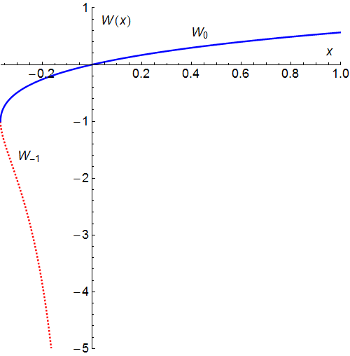
In this appendix we repeat some basic properties of the Lambert W-function that we use in our paper. The W-function is defined implicitly as follows:
The W-function has two real branches, namely for and for . These are separated by a branch point at . For a plot of the real branches, see figure 14. The Taylor expansion of the W-function around the point , in each of the two branches is [30]:
The unsigned Stirling numbers of the first kind are defined recursively as follows:
Appendix E Elliptic Integrals and Jacobian Elliptic Functions
This appendix provides the definitions, the Taylor series and some of the properties of elliptic integrals and Jacobian elliptic functions. For details, the reader is referred to the handbook [31].
Jacobian Elliptic Functions
Elliptic Integral of the First Kind
where is the digamma/psi function.
Elliptic Integral of the Second Kind
Elliptic Integral of the Third Kind
The following addition formula of complete elliptic integrals of the third kind can be found in [32]:
References
- [1] C. Kristjansen, M. Staudacher, and A. Tseytlin, Gauge-String Duality and Integrability: Progress and Outlook, J. Phys. A42 (2009) 250301.
- [2] N. Beisert et al., Review of AdS/CFT Integrability: An Overview, Lett.Math.Phys. 99 (2012) 3, [arXiv:1012.3982].
- [3] C. Marboe and D. Volin, Quantum Spectral Curve as a Tool for a Perturbative Quantum Field Theory, Nucl.Phys. B899 (2015) 810, [arXiv:1411.4758].
- [4] N. Gromov, F. Levkovich-Maslyuk, G. Sizov, and S. Valatka, Quantum Spectral Curve at Work: from Small Spin to Strong Coupling in SYM, JHEP 07 (2014) 156, [arXiv:1402.0871].
- [5] N. Gromov, V. Kazakov, S. Leurent, and D. Volin, Quantum Spectral Curve for Planar Super Yang-Mills Theory, Phys.Rev.Lett. 112 (2014) 011602, [arXiv:1305.1939].
- [6] K. Zarembo, Spin Chains and Strings in Gauge Theory, 2008. Talk at the AlbaNova and Nordita Colloquium.
- [7] R. Roiban, A. Tirziu, and A. A. Tseytlin, Slow-String Limit and ”Antiferromagnetic” State in AdS/CFT, Phys.Rev. D73 (2006) 066003, [hep-th/0601074].
- [8] K. Okamura, Giant Spinons, JHEP 04 (2010) 033, [arXiv:0911.1528].
- [9] J. A. Minahan and K. Zarembo, The Bethe-Ansatz for Super Yang-Mills, JHEP 03 (2003) 013, [hep-th/0212208].
- [10] D. Berenstein, J. Maldacena, and H. Nastase, Strings in Flat Space and pp Waves from Super Yang Mills, JHEP 04 (2002) 013, [hep-th/0202021].
- [11] S. S. Gubser, I. R. Klebanov, and A. M. Polyakov, A Semi-Classical Limit of the Gauge/String Correspondence, Nucl.Phys. B636 (2002) 99, [hep-th/0204051].
- [12] D. M. Hofman and J. Maldacena, Giant Magnons, J.Phys. A39 (2006) 13095, [hep-th/0604135].
- [13] K. Zarembo, Antiferromagnetic Operators in Supersymmetric Yang-Mills Theory, Phys.Lett. B634 (2006) 552, [hep-th/0512079].
- [14] N. Beisert, V. Dippel, and M. Staudacher, A Novel Long-Range Spin Chain and Planar Super Yang-Mills, JHEP 07 (2004) 075, [hep-th/0405001].
- [15] N. Beisert, The Dynamic S-Matrix, Adv.Theor.Math.Phys. 12 (2008) 945, [hep-th/0511082].
- [16] G. Papathanasiou and M. Spradlin, Semiclassical Quantization of the Giant Magnon, JHEP 06 (2007) 032, [arXiv:0704.2389].
- [17] H.-Y. Chen, N. Dorey, and R. F. Lima Matos, Quantum Scattering of Giant Magnons, JHEP 09 (2007) 106, [arXiv:0707.0668].
- [18] G. Arutyunov, S. Frolov, and M. Zamaklar, Finite-Size Effects from Giant Magnons, Nucl.Phys. B778 (2007) 1, [hep-th/0606126].
- [19] D. Astolfi, V. Forini, G. Grignani, and G. W. Semenoff, Gauge Invariant Finite Size Spectrum of the Giant Magnon, Phys.Lett. B651 (2007) 329, [hep-th/0702043].
- [20] E. Floratos and G. Linardopoulos, Large-Spin and Large-Winding Expansions of Giant Magnons and Single Spikes, Nucl.Phys. B897 (2015) 229, [arXiv:1406.0796].
- [21] G. Linardopoulos, Classical Strings and Membranes in the AdS/CFT Correspondence. PhD thesis, National and Kapodistrian University of Athens, 2015. http://www.didaktorika.gr/eadd/handle/10442/35838?locale=en.
- [22] G. Linardopoulos, Large-Spin Expansions of Giant Magnons, PoS (CORFU2014) 154, [arXiv:1502.01630].
- [23] R. Ishizeki and M. Kruczenski, Single Spike Solutions for Strings on S2 and S3, Phys.Rev. D76 (2007) 126006, [arXiv:0705.2429].
- [24] A. Mosaffa and B. Safarzadeh, Dual Spikes: New Spiky String Solutions, JHEP 08 (2007) 017, [arXiv:0705.3131].
- [25] H. Hayashi, K. Okamura, R. Suzuki, and B. Vicedo, Large Winding Sector of AdS/CFT, JHEP 11 (2007) 033, [arXiv:0709.4033].
- [26] C. Ahn and P. Bozhilov, Finite-Size Effects for Single Spike, JHEP 07 (2008) 105, [arXiv:0806.1085].
- [27] E. Floratos, G. Georgiou, and G. Linardopoulos, Large-Spin Expansions of GKP Strings, JHEP 03 (2014) 018, [arXiv:1311.5800].
- [28] M. Axenides, E. Floratos, and G. Linardopoulos, Stringy Membranes in AdS/CFT, JHEP 08 (2013) 089, [arXiv:1306.0220].
- [29] M. C. Abbott and I. V. Aniceto, Vibrating Giant Spikes and the Large-Winding Sector, JHEP 06 (2008) 088, [arXiv:0803.4222].
- [30] R. M. Corless, G. H. Gonnet, D. E. G. Hare, D. J. Jeffrey, and D. E. Knuth, On the Lambert W Function, Adv.Comput.Math. 5 (1996) 329.
- [31] M. Abramowitz and I. Stegun, eds., Handbook of Mathematical Functions. Dover, New York, 1972.
- [32] P. F. Byrd and M. D. Friedman, Handbook of Elliptic Integrals for Engineers and Scientists. Springer-Verlag, 1971.