DataGrinder: Fast, Accurate, Fully non-Parametric Classification Approach Using 2D Convex Hulls

Abstract

It has been a long time, since data mining technologies have made their ways to the field of data management. Classification is one of the most important data mining tasks for label prediction, categorization of objects into groups, advertisement and data management. In this paper, we focus on the standard classification problem which is predicting unknown labels in Euclidean space. Most efforts in Machine Learning communities are devoted to methods that use probabilistic algorithms which are heavy on Calculus and Linear Algebra. Most of these techniques have scalability issues for big data, and are hardly parallelizable if they are to maintain their high accuracies in their standard form. Sampling is a new direction for improving scalability, using many small parallel classifiers. In this paper, rather than conventional sampling methods, we focus on a discrete classification algorithm with $O(n)$ expected running time. Our approach performs a similar task as sampling methods. However, we use column-wise sampling of data, rather than the row-wise sampling used in the literature. In either case, our algorithm is completely deterministic. Our algorithm, proposes a way of combining 2D convex hulls in order to achieve high classification accuracy as well as scalability in the same time. First, we thoroughly describe and prove our $O(n)$ algorithm for finding the convex hull of a point set in 2D. Then, we show with experiments our classifier model built based on this idea is very competitive compared with existing sophisticated classification algorithms included in commercial statistical applications such as MATLAB.

1 Introduction

Data mining topics such as classification [1, 2, 14, 15, 19, 24, 25, 29], clustering [38, 28, 27, 26, 24, 8, 7, 5, 3], frequent pattern mining [37, 36, 11], frequent sub-structure mining [11, 24], regression [21, 20], data cleaning [18, 8, 1], ranking [6], data warehousing [5], recommender systems [23, 16, 10], bio-informatics [19], outlier detection [22, 13, 4], nearest neighbors [17, 9] and social networks [31, 32], have been widely discussed in data management and prediction. There has been plenty of work on classification as one of the main techniques for supervised learning. Figure 1, shows a small example where we have sets of points in a plane, each of which belonging to one category, demonstrated by different shapes. A classifier model, is given data vectors in 2 dimensional space (2D), with labels (i.e. training), and is expected to predict, and assign new objects with missing labels to their correct categories(i.e. testing).

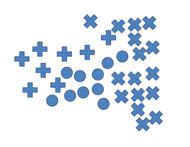
Figure 1: Classification Example with 3 Classes

There exist a variety of classification algorithms in machine learning and data mining. Most popular classifiers are known as discriminant classifiers. Discriminant classifiers aim at statistical or probabilistic modeling in order to find an objective function. Then, optimization and numerical methods are used in order to find optimal parameter values. Having found these optimal values, we can find the decision boundaries that divide the space into regions that separate objects from different categories. It is often the case that data is not linearly separable. This leads to misclassification errors most of the times. In order to minimize misclassification error, people use methods such as regularization, kernel transformations, feature extraction and feature selection [39]. Examples of discriminant classifiers include Support Vector Machines and Logistic Regression [2, 29].

Other types of classifiers are Decision Trees, Rule-based [33, 34, 35] methods and Nearest Neighbor methods. Most of these methods have practical shortcomings. Discriminant classifiers need to optimize their objective function and this may not be feasible in reasonable time for big data. Besides, it is a challenge to find straight forward parallel implementations of these optimization algorithms. In web-based scenarios, data changes very frequently [24]. This requires either algorithms with highly scalable training phase, or models we can sequentially update. Although time always plays a key role and sometimes sequential update may not be optimal [30]. Decision Trees and Rule-based classifiers also suffer from the same shortcoming in practical scenarios. In many cases, the theoretical problem defined to solve the classification problem is NP-hard. Nearest Neighbor methods are efficiently applicable if data is stored in data structures such as kd-trees for nearest neighbor search. Despite their efficiency in execution, they lack accuracy even for slightly challenging inputs. We demonstrate this with experiments in Section 6, and briefly explain how each classification algorithm works.

In this paper, rather than solving optimization problem, we use Computational Geometry, in order to build an accurate classifier. We use 2D convex hulls, using all possible 2 dimensional projections (i.e. all possible pairs of columns regardless of order). Figure 2(a), shows an example of the convex hull of a point set $P$. In order to build classifiers, we project the input dataset with $d$ dimensions to all possible $\binom{d}{2}$ planes. In each plane, having partitioned the training data into different classes, we find the 2D convex hull for each class (Select-Project-ConvexHull). This results in $C\times\binom{d}{2}$ convex hulls, where $C$ is the number of classes. Given a new testing instance with $d$ feature values, we check for all existing $C\times\binom{d}{2}$ convex hulls, whether they contain the corresponding $2$ dimensional projection($\pi$). We find the class $c_{max}$, that scores highest (i.e. its boundaries contain the point in more 2D projections) and assign the class label. Since $d$ is typically a small constant in practice, we are not worried about the testing time. Besides, using parallelization, testing time is negligible. We also propose a filtering approach to choose only the most discriminant features in Section 6, that results in accuracy improvements as well. We explain our classification algorithm in more detail in Section 5, after providing the necessary computational geometry background. We make the following contributions in this paper:

1. We explain the Convex Hull problem from Computational Geometry [40]. We provide algorithmic background in terms of the running time, and propose an algorithm with $O(n)$ expected running time. We also prove its correctness. Besides, we calculate the "constant" through probabilistic analysis, and our experiments show our calculated constant is reliable for different sizes of data. Database community has shown tremendous interest in solving problems formulated similar to convex hulls such as designing algorithms for finding Skylines [22, 13, 4].

2. We propose and explain our classification algorithm, DataGrinder(DGR), using 2D convex hulls. We also propose tricks for tuning the classifier by filtering weak features that results in considerable accuracy improvement, in the case of one dataset.

3. We propose parallel algorithms for implementing DataGrinder at different levels including data partitioning as well as parallel convex hull algorithms, using the divide and conquer method.

4. We propose a method for random data generation and testing classifiers. Our proposed testing methodology controls the hardness of classification using two parameters. We conduct a comprehensive set of experiments on randomly generated and real datasets. Our experiments show DataGrinder is competitive against the most widely known commercial classifiers in accuracy, while being extremely scalable.

2 Convex Hull Background

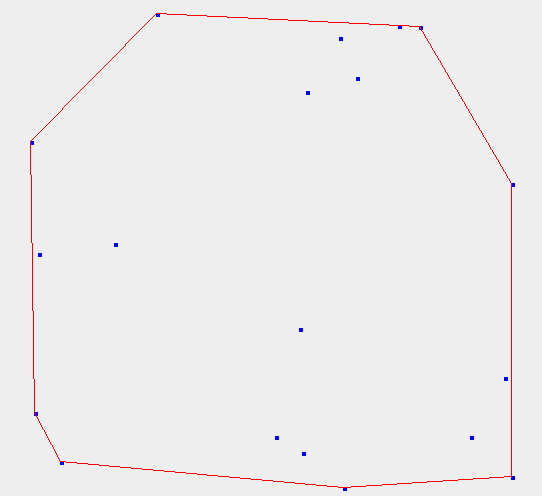
(a) Convex Hull of $P$

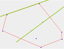
(b) Convex Hull and Line Segments

Figure 2: Convex Hull of a point set $P$. The set of all line segments that have every other point only in one of their half spaces is a polygon that is called the convex hull $CH(P)$.

Convex Hull of a point set in 2D, $CH(P)$, is a set of points such that every point in $P$ can be computed as a positive linear combination (all the weights are positive), of the points in $CH(P)$. For this reason, it is important in applications where we are interested in finding mixtures using some baseline prototype vectors. In a sense, convex hull of a point set is a small subset of the points that wraps around a point set, and can represent any point in the point set with a positive linear combination. We can represent convex hull as a polygon, that contains every other point in $P$, within its boundaries. This polygon that wraps around all points can be extremely useful for applications in Machine Learning when we want to define the boundaries of a group of points (class). It also has the base ingredients to represent any point in that class. For instance, we can use convex hull along with radial basis or any other sort of function in order to construct a kernel and represent every point in a new feature space.

Moreover, in Computational Geometry, problems such as finding half space intersection can be reduced to finding convex hull and this highlights the importance of exploring more computationally efficient algorithms. In many real life applications we deal with datasets with thousands or millions of data points, and existing $O(nlog(n))$ algorithms fail to find convex hull in a timely manner. Other than problems we can directly model with convex hull, there are many other domains such as web mining where we deal with large graphs. We can also use properties of these domains such as link structure in order to define entities such as web pages in a multidimensional Euclidean space, and use convex hull for modeling [24].

We only focus on the 2D case but our heuristics and ideas are generalizable to higher dimensions. We use 2D for simplicity because it is more intuitive for problem solving and leave generalized version to our future work. Moreover, in our present application of convex hulls (i.e. classification), we are seeking data boundaries as tight as possible while still maintaining properties of binary feature correlations. This, kind of resembles entries of a covariance matrix, in Multivariate Gaussian Distributions that can be used for Principle Component Analysis as well.

It is provable that the best possible worse case running time for this problem is $O(nlog(n))$, since sorting can be reduced to the convex hull problem [40]. In fact, the most efficient classic convex hull algorithms use sorting. First, we sort all the points in a dataset according to one coordinate. Then, using a left to right scan of the sorted list, we iterate over other points and remove any points that do not belong to the convex hull, in linear time. In order to do so, they use geometric properties of the points on convex hull and line segments between them. Figure 2(a) shows a point set along with a polygon that wraps around it. If we extend each line segment in both ends, we obtain a line such that every other point in $P$, is located on one side (i.e. half space).

We devise an algorithm, that despite its $O(n^{2})$ worst case running time, achieves $O(n)$ expected running time if $P$ is distributed uniformly, and dimensions are independent. We also prove for independent Normal distributions. Previous work in Computational Geometry also approves the possibility of $O(n)$ expected running time, if the algorithm is designed within the given framework [41]. Here, we thoroughly describe the algorithm and provide pseudo code as well as average case analysis for computing the constant. Regardless of the data instance, we can always devise strategies to avoid the worst case through smart query optimization, and use of empirical algorithms.

Our 2D convex hull algorithm avoids paying the initial $nlogn$ sorting time. Instead, in every iteration our new algorithm finds the next minimum of the list in $O(|candidates|)$, and using the new point, it uses a heuristic to remove other points from the candidate set, that do not qualify to be on convex hull. This is what we refer to as Candidate Elimination process. Once we process all the candidates and remain with an empty candidate set, we have found the convex hull. Our theoretical analysis as well as our quantitative experimental results, suggest that repeating this process results in $O(n)$ expected running time, for finding 2D convex hull. This iterative candidate elimination process enables us to find the convex hull of up to $1000000$ points in less than $20$ seconds while the existing classic algorithm fails to terminate in in a timely manner (after 8 hours). It is worth highlighting again that although the classic algorithm has a better worst case running time, it fails in practice. In the rest of this section, we formally define the convex hull problem and discuss naive and classic solutions. In the subsequent subsections, we discuss a new algorithm based on candidate elimination, and discuss its expected running time. Eventually, we show with experiments that the improvement achieved using this pruning heuristic is indeed considerable, and indeed it results in linear expected running time.

2.1 Convex Hull Problem Definition

Convex Hull of a point set $P=\{p_{1},p_{2},...,p_{n}\}$, is best defined intuitively as a polygon that wraps around all the points in $P$. We can formally define this polygon as follows.

DEFINITION 1

Convex Hull of a point set, $CH(P)$, is the set of all line segments, $pq$, between every two pair of points from $P$, such that every other point is located on one side of $pq$. We can also use negative or positive, in order to refer to these two "half spaces". In other words, every other point either belongs to the negative half space, or to the positive half space.

Naive algorithm for finding $CH(P)$ is as follows:

• Produce every pair of points $p_{i}$ and $p_{j}$: $O(n^{2})$

• Find the line segment between $p_{i}$ and $p_{j}$ in constant time.

• Check if every other point belongs to either negative or positive half space. If yes, add the line segment to $CH(P)$ otherwise discard: $O(n)$.

Figure 2(b), shows examples of both types of line segments. Overall running time of the naive algorithm is $O(n^{3})$, since it scans $P$ once for every pair of points. This results in a process that takes minimal usage of geometric properties and is extremely inefficient. Using geometric properties, we can aim at designing a more targeted process. Next, we describe $O(nlog(n))$ algorithm that first sorts all the points by their $x$-coordinate.

2.2 Background of Algorithms ($nlogn$ algorithm)

Rather than arbitrarily exploring the search space, first we sort the point set based on one coordinate (typically $x$). Points in $P$, start from $X_{min}$ and end at $X_{max}$ after sorting.

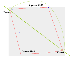
Figure 3: Upper and Lower Hulls between $X_{min}$ and $X_{max}$.

Figure 3, splits the convex hull into two parts, both from $X_{min}$ to $X_{max}$. We use Upper Hull ($UH$), in order to refer to the part above the line segment between $X_{min}$ and $X_{max}$; we use Lower Hull ($LH$), in order to refer to the lower part. Classic algorithm for finding convex hull invokes $FindUpperHull(P)$ and $FindLowerHull(P)$ functions, in order to find the convex hull of $P$, each in $O(n)$. Therefore, the total execution time is $O(nlog(n))$. Finding upper and lower hulls separately are two symmetric procedures with respect to each other. Here, we only present for upper hull. Algorithm 1, computes the upper hull of the sorted point set by scanning from $X_{min}$ to $X_{max}$. It is intuitive that we visit all the points in $UH(P)$ in sequence, once we do scanning from left to right, although with the rest of the points in between. The idea is to: 1) perform this scanning; 2) identify and maintain points that belong to $UH(P)$, and 3) discard all the other points. We change $i$ from $1$ to $n$, and start the $i^{th}$ iteration having computed the correct upper hull of the points $\{p_{1}...p_{i-1}\}$. We add $p_{i}$ to $UH(P)$, because we know it belongs to the upper hull of $\{p_{1}...p_{i}\}$, with the largest $x-$coordinate value so far. We read $UH(P)$ in reverse order and remove any points that do not belong to the convex hull of $\{p_{1}...p_{i}\}$, until we stop.

0:  Point set $P$, sorted by $x-$coordinate

0:  Upper hull of $P$, $UH(P)$

1:  $UH=$ initialize empty

2:  for $i=1$ to $n$ do

3:     $UH.append(p_{i})$

4:     $\ell=i$

5:     while $(\ell>2)$&&$(!UHCheck(p_{\ell-2},p_{\ell-1},p_{\ell}))$ do

6:        remove $p_{\ell-1}$ from $UH$

7:        $\ell=\ell-1$

8:  return $UH$

Algorithm 1 FindUpperHull$(P)$

After appending $p_{i}$ to $UH$, we check for the last $3$ points in $UH$, if they belong to the correct convex hull or not. In order to do so, $UHCheck(p_{\ell-2},p_{\ell-1},p_{\ell})$ returns true if $p_{\ell-1}$ is above the line segment from $p_{\ell-2}$ to $p_{\ell}$. This means $p_{\ell-1}$ belongs to $UH_{i}$. Otherwise, it is removed and we repeat this process until $UHCheck$ returns true, and obtain the correct upper hull of $p_{1}$ to $p_{i}$. Equation 1, computes a sign variable. If sign is a non-negative number, $UHCheck$ returns true.

$$\begin{array}[b]{r}sign=(p_{\ell-1}.y-p_{\ell-2}.y)(p_{\ell}.x-p_{\ell-2}.x)-\\ (p_{\ell-1}.x-p_{\ell-2}.x)(p_{\ell}.y-p_{\ell-2}.y)\end{array}$$ (1)

Figure 4, shows a snapshot during the execution, where two middle points need to be removed after adding $p_{5}$. It also shows the correct upper hull after we exit the while loop. We exit the while loop when for the first time we find a middle point which passes the convex test (Equation 1). When this happens, it is guaranteed that $UH_{5}(P)$ is convex since the last step is convex and also we know the rest is constructed convex starting from $p_{1}=X_{min}$. We exit the while loop also when only $2$ points are left, in which case there is no middle point and $UH_{i}(P)$ is always convex.

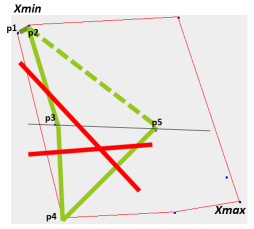
Figure 4: A snapshot of running the classic algorithm for finding upper hull. Convex Hull of $p_{1}...p_{4}$ is constructed by adding the points one by one without removing any points. When $p_{5}$ is added, $p_{4}$ needs to be removed because upper hull of $p_{1}...p_{5}$ is not convex anymore. Moving backwards iteratively, FindUpperHull (Algorithm 1), removes $p_{4}$ and $p_{3}$ and we remain with $UH_{5}(P)=\{p_{1},p_{2},p_{5}\}$.

It is worth noting, it can happen that two points appear in sorted $P$ next to each other with the same value for $x-$coordinate. In this situation, we order all the points with the same $x-$value based on their $y-$coordinate to preserve the correctness of Algorithm 1. If two points are exactly the same, one can be removed without hurting the correctness of the convex hull algorithm.

3 Finding Convex Hull by Candidate Elimination

Classic convex hull algorithm presented so far needs to perform an initial sorting with cost $O(nlog(n))$. We know we can not do better in the worst case for finding convex hull. Despite $O(nlog(n))$ worst case running time, in many cases we may be able to use heuristics in order to make the problem size smaller and achieve better Expected running time. In this section, we describe a process called "Candidate Elimination", that we use, instead of sorting. We use candidate elimination along with existing FindUpperHull procedure, in order to solve the problem. The idea is to avoid sorting, maintain candidate lists of points for different parts of the convex hull, and find the next minimum value from a smaller candidate list, rather than paying $O(nlog(n))$ for sorting in the beginning.

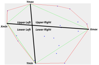
Figure 5: Dividing the plane into 4 quarters using $X_{min}$, $X_{max}$, $Y_{min}$ and $Y_{max}$.

Figure 5, divides the plane as well as the convex hull of the point set into $4$ quarters, using minimum and maximum $x$ and $y$ values in the point set. We use $UpperLeftHull$, $UpperRightHull$, $LowerLeftHull$ and $LowerRightHull$, in order to refer to these $4$ quarters.

LEMMA 1

All of the points on $UpperLeftHull$ are on or above the line from $X_{min}$ to $Y_{max}$.

Proof 3.1.

We know the upper left hull starts at $X_{min}$ and ends at $Y_{max}$. We also know that the upper left hull is convex. Therefore, none of the points on it can be below the line.

Lemma 1, provides an opportunity for candidate elimination in the beginning. We can draw a line from $X_{min}$ to $Y_{max}$, and remove any points below the line, to obtain a list of $UpperLeftHull$ candidates. Using symmetry, we can find a candidate list for $UpperRightHull$ by choosing all the points above the line that goes through $Y_{max}$ and $X_{max}$. Lower left candidates are those on or below the line from $X_{min}$ to $Y_{min}$, and lower right candidates are on or below the line from $Y_{min}$ to $X_{max}$. Finding minimum and maximum $x$ and $y$ coordinate values can be done in $O(n)$. Therefore, by paying $O(n)$, we can discard many points and continue with smaller input size and this obviously can considerably improve the performance. We use Candidate Elimination, to refer to this process that makes more targeted use of both $x$ and $y$ coordinates. Figure 6, shows a minimal box that contains all of the points in $P$, using $X_{min}$, $X_{max}$, $Y_{min}$ and $Y_{max}$. Inside this box, we separate $4$ triangles in $4$ corners. These are the only areas where convex hull candidates can appear. We use Candidate Area in order to refer to any area inside the box, where convex hull candidates can appear. In Figure 6, four triangles form the candidate area.

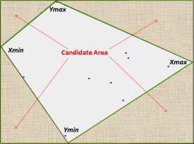
Figure 6: Box area vs. Candidate Area.

LEMMA 2

The expected number of candidates after the first candidate elimination is $n/2$.

Proof 3.2.

We assume points are distributed uniformly in the plane. We also assume that $x$ and $y$ coordinates are uniform and independent. Given these assumptions, we define $z_{i}$ to be a random variable. We assign $z_{i}=1$, if the $i^{th}$ point in $P$ is in the candidate area. We know $P(z_{i}=1)=(CandidateArea/BoxArea)=1/2$; therefore, $E(z_{i})=1/2$. There are $n$ such points in the dataset, and we can use $E(Z)=\sum_{i=1}^{n}E(z_{i})$ while $Z$ is a random variable that takes values in $\{1...n\}$, that indicates the number of candidate points all together after the first candidate elimination. Expected value of $Z$ is $n$ times expected value of $z_{i}$, equal to $n/2$, using linearity of expected value.

3.1 Convex Hull Algorithm

The first candidate elimination step reduces the expected number of candidates to half. Although this is a good heuristic, we still need to eliminate more candidates, and find the correct convex hull. As described earlier, we do this in $4$ smaller steps for $UpperLeftHull$, $UpperRightHull$, $LowerLeftHull$, and $LowerRightHull$, separately. Here, we only describe the process for $UpperLeftHull$, and we know the rest is symmetric for the three other quarters of the convex hull. Algorithm 2, takes as input the list of upper left candidates after the initial candidate elimination, that are on or above the line from $X_{min}$ to $Y_{max}$. Please note, that the list is not sorted by $x-$coordinate anymore. The idea is to avoid sorting the candidate list. Instead, we keep finding the next smallest $x$, $NextX$, and repeat candidate elimination using $NextX$. The justification behind replacing sorting with this operation, is the fact that candidate list keeps getting smaller and smaller after performing candidate eliminations in sequence. This makes the cost of finding the next minimum negligible, even for large $n$.

0:  $ULCandidates$, list of candidates for upper left hull

0:  Upper left hull of $P$, $ULH(P)$

1:  $ULH=$ initialize empty

2:  while $ULCandidates.size>0$  do

3:     $NextX=removeLeftMostPoint(ULCandidates)$

4:     $eliminateCandidates(ULCandidates,NextX,Y_{max})$

5:     $ULH.append(NextX)$

6:     $\ell=ULH.size$

7:     while $(\ell>2)$&&$(!UHCheck(p_{\ell-2},p_{\ell-1},p_{\ell}))$ do

8:        remove $p_{\ell-1}$ from $ULH$

9:        $\ell=\ell-1$

10:  return $ULH$

Algorithm 2 FindUpperLeftHull$(ULCandidates)$

Rather than reading the next point from sorted $P$, in order to find upper left hull, Algorithm 2, finds $NextX$ in line $3$ and removes it from the list of upper left candidates. We pay $O(|ULCandidates|)$ cost to find $NextX$. In line $4$, $eliminateCandidates$ repeats the same candidate elimination task using $NextX$. In order to do so, we draw a line from $NextX$ to $Y_{max}$, and remove any candidates below the line. In the rest of Algorithm 2, we pretend $NextX$ is read from a sorted list and repeat the same process in order to fix $UpperHull$ that Algorithm 1 does, already presented in Section 2.2.

4 Running Time Analysis

4.1 Worst Case Running Time

There are three main steps in each iteration of finding convex hull by candidate elimination:

• Finding $NextX$, overall $O(|candidates|)$

• Candidate elimination, $O(|candidates|)$

• Fixing upper hull, $C$ (constant)

It is possible in the worst case, that all of the points in $P$ belong to the convex hull. In this case, candidate elimination results in removing no candidates and repeating a $O(n)$ process $n$ times, resulting in $O(n^{2})$ worst case running time. For the current classification problem, worst case scenario rarely happens.

4.2 Expected Running Time

Since there are $4$ quarters and the expected number of candidates is $n/2$ after the initial candidate elimination, there is an expected number of $n/8$ candidates in each triangle. It is worth noting, we can use the product of expected values of two random variables as the expected value of their product, because all the random variables are independent . This, is a natural assumption, used widely in Machine Learning [39]. We define $\alpha_{0}=1/8$ to be the elimination ratio, indicating the expected cost of finding $NextX$, after the initial candidate elimination in each quarter. We present using $LowerRightHull$, to have more variety in our examples. Subsequently, we can define, $0<\alpha_{1}<1$, as elimination ratio in iteration $1$ and, $0<\alpha_{2}<1$, as elimination ratio in iteration $2$. The expected size of $LRCandidates$ after iteration $2$ is $(\alpha_{0}\alpha_{1}\alpha_{2})\times n$.

LEMMA 3

Expected running time of finding the convex hull of the lower right quarter is $n/8\times(\sum_{i=1}^{n/8}(\prod_{j=1}^{i}\alpha_{j}))$.

Proof 4.1.

We know $\alpha_{0}$ is the initial elimination ratio that reduces the number of lower right candidates to $n/8$. Therefore, this is the expected size, we start with. In each iteration, we pay the cost $O(|LRCandidates|)$. The number of $LRCandidates$ after iteration $2$, is $\alpha_{1}\alpha_{2}\times n/8$. Similarly, the number of candidates after the $i^{th}$ iteration is $\prod_{j=1}^{i}\alpha_{j}$. Therefore, we pay $n/8\times\prod_{j=1}^{i}\alpha_{j}$ cost, which is the expected size of $LRCandidates$. Adding up for a maximum of $n/8$ iterations we get $(\sum_{i=1}^{n/8}(\prod_{j=1}^{i}\alpha_{j}))$, the total expected cost of finding $LowerRightHull$. Although we write the sum for $n/8$ iterations, it is quite likely that in the end the expected cost is $0$ or close to $0$. This is because an exponentially smaller coefficient is multiplied by $n/8$. This is because all $\alpha_{1}...\alpha_{n/8}$ are smaller than $1$.

LEMMA 4

$\alpha$ is a decreasing function that approaches $3/4$.

Proof 4.2.

Suppose at some iteration we have found $NextX$ and we perform candidate elimination. Figure 7, compares candidate area to eliminated area. Candidate area is shown below the line from $NextX$ to $X_{max}$. Eliminated area is a triangle with $area=ac/2$. Total area is $bc/2+ac+ac/2$. Therefore, $\alpha=(bc/2+ac)/(bc/2+ac+ac/2)=(2a+b)/(3a+b)$. As we get closer to $X_{max}$, $b$ gets closer to $a$ and the value of $\alpha$ decreases to $3a/4a=3/4$.

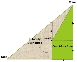
Figure 7: Candidate elimination after finding $NextX$

Using lemma 4, we know $(\prod_{j=1}^{i}\alpha_{j})$ is a product that decreases with $i$. Since $\alpha$ is smaller than $1$ all the time, and $\alpha$ is a decreasing function. We can "assume" $(\prod_{j=1}^{i}\alpha_{j})$ exponentially decreases with $i$ and we can bound the expected running time using the sum of a geometric series as follows: $n/8\times\sum_{i=1}^{n/8}\bar{\alpha}^{i}$. Since $\bar{\alpha}$ is a constant between $0$ and $1$, we know the sum of the geometric series is constant and so is the expected running time. We know minimum value for $\alpha$ is $3/4$ and $\alpha<1$. Using average value of $3/4$ and $1$, we can approximate $\bar{\alpha}=7/8$, resulting in $O(n)$ points accessed during the execution of the convex hull algorithm for each corner. Finally, we can approximate $4n$ as the total number of points accessed during the execution for finding the convex hull of $4$ quarters. Next, we aim at calculating a constant upper bound for the expected cost, in order to prove the expected cost is linear, when convex hull is found by candidate elimination, instead of using $\bar{\alpha}$ which is only raw approximation!

THEOREM 1

The expected value of $\alpha_{1}$ is constant $<1$ and expected running time is bounded by the sum of $\alpha_{1}$’s geometric series.

Proof 4.3.

In order to choose $NextX$, we need to draw a point from the uniform distribution specified by the triangle in Figure 7. The three corners of the triangle have these coordinates:$(Y_{min}.x,Y_{min}.y)$, $(X_{max}.x,Y_{min}.y)$,
$(X_{max}.x,X_{max}.y)$. We are interested in finding the expected position of $NextX$ on $x-$axis. Since the distribution is uniform and we are interested in expected $NextX.x$, we need to find the point on $x-$axis, such that if we split the triangle using a vertical line, candidate areas inside the triangle on both sides of the vertical line are equal. We assume the perpendicular sides of the triangle have equal expected length. One is equal to $L1=X_{max}.x-Y_{min}.x$, and the other equal to $L2=X_{max}.y-Y_{min}.y$. $L1$ and $L2$ are two random variables. $E(L1/L2)$ depends on the range of values of $x$ and $y$ coordinates in the point set. It is usually the case that these coordinates are either in the same range or we can perform normalization and make expected values of $L1$ and $L2$ both equal to a value $L$. Thus, without loss of generality we calculate $(L-c)^{2}/2$ as the triangle area on the left side of $NextX$. We also compute $(2L-c)\times c/2$, the area inside the triangle on the right side of $NextX$. Therefore, we need to find the value of $c$ in terms of $L$ in the following equation:

$$L^{2}+c^{2}-2Lc=2Lc-c^{2}$$

.

We get $c=L/(2+\sqrt{2})=L/3.4\approx 0.3L$, by solving the above equation. After drawing a large enough (constant) number of points from the distribution, we can assume the expected value is reached in any instance of the problem. If we rewrite $\alpha=(2a+b)/(3a+b)$ that we computed earlier in the proof of lemma 4, in terms of $L$ and $c$, and replace $c=0.3L$, we get $a\approx 0.35L$, $b\approx 0.65L$ and $\alpha=0.79$. Therefore, we can bound expected running time by $(1/(1-0.8))\times n=5n$. We need to do an initial scanning of the list in the first candidate elimination and read $n$ points. Therefore, we compute $6n$ as an upper bound for the expected number of points read during the execution.

Regardless of the exact running time, by proving Theorem 1, we have shown the expected running time of the algorithm is $O(n)$. In the next section, in our experiments we use counters for the number of points read until we find the convex hull for each experiment. In all of our experiments, we read almost $4n$ points during execution. This emphasises, the importance and reliability of our theoretical analysis for computing the expected running time in this section.

THEOREM 2

Expected running time is linear if $P$ follows a Normal distribution.

Proof 4.4.

We have already done the proof for Uniform distribution. We know Normal distribution is more centered around its mean and further from its boundaries. It is obvious that this results in more probability mass in eliminated areas in all of the proofs regarding the expected running time analysis. We can say the expected running time when $P$ is Uniform is an upper bound for the expected running time when $P$ is Normal.

4.3 ConvexHull Running Time: Experimental Analysis

We performed $6$ experiments for different number of points in $P$. The number of points grows exponentially. In all cases, we generate the point set randomly from uniform distribution. We use $ClassicAlg$ for the classic algorithm and $NewAlg$ for our new algorithm based on candidate elimination. We use $QuickSort$ with expected $O(nlog(n))$ time for sorting in the implementation of classic algorithm which is typically one of the most efficient in practice. In all cases, except for $n=10$, our running time is almost $4n$. In the case of $n=10$, we perform $68$ point reads which is more than $40$. Although the difference is negligible, we relate the additional cost paid to the overhead of finding four quarters of the convex hull separately. There exists a negligible amount of overhead because $X_{min}$, $X_{max}$, $Y_{min}$ and $Y_{max}$ belong to candidate sets in more than $1$ quarters.

$\#Points$	$10$	$10^{2}$	$10^{3}$	$10^{4}$	$10^{5}$	$10^{6}$
$ClassicAlg.$	$145$	$2367$	$32425$	$474853$	$14462151$	?
$NewAlg.$	$68$	$424$	$4237$	$39854$	$398406$	$3879651$

The remarkable results we observe in the above table are: 1) Linear number of point reads compared to the input size for our new algorithm; 2) Finding $2-$D convex hull of up to $10^{6}$ points while the classic algorithm fails to do so. We also notice we pay a lot less cost in order to find the convex hull of $10^{6}$ points than the classic algorithm pays to find the convex hull of $10^{5}$ points.

5 Classification Algorithm

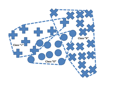
Figure 8: Convex Hull used as a boundary for each class. Convex Hulls may partially overlap.

Figure 8, shows the same distribution of data in classes as Figure 1. It also shows how classes are separated using their 2-dimensional (2D) convex hulls. Any new sample with missing label is checked against these three convex hulls. It is classified in that class if it is inside the corresponding convex hull. As shown in the figure, these classes overlap in the areas they cover and misclassification is always possible. It is also the case that if we try to separate these classes using other decision boundaries we face the same problem. Since convex hull tightly wraps around the points from each class, it reduces the chances of misclassification using its tight boundaries. There can be instances where the point falls outside all convex hulls. In such cases, we can assign a point to a class using it’s proximity in Euclidean space. In the rest of this paper, we only deal with classification problems where there are typically $d>2$ features. In this case, since there are more than 2 dimensions, for each class we produce 2D convex hulls for every permutation of 2 features resulting in $\binom{d}{2}$ convex hulls for $d$ features. We define the notion of 2DAspect as follows:

DEFINITION 2

A two dimensional data aspect
(2DAspect) is a structure containing the following data.

• ClassLabel (String): the class this 2DAspect belongs to.

• $f_{1}$, $f_{2}$ (int): indices of a pair of features chosen from the set of all possible pairs.

• UpperHull: ordered list of points that form the upper hull of data in $f_{1}$,$f_{2}$ plane.

• LowerHull: ordered list of points that form the lower hull of data in $f_{1}$,$f_{2}$ plane.

In order to check whether a point is covered by a 2DAspect, we check if it is below all the lines on the UpperHull and above all the lines on the LowerHull. Our convex hull based classifier, is composed of $C\times\binom{d}{2}$ 2DAspect’s, while $C$ is the number of classes. Algorithm 3, provides the pseudo-code for training a DataGrinder using 2D convex hulls.

0:  $X_{n\times d}$ data matrix, $Y_{n\times 1}$ corresponding labels of rows in $X$.

0:  All $C\times\binom{d}{2}$ two dimensional aspects

1:  $2DAspects=$ empty list

2:  for each class $C_{i}$  do

3:     for each pair of features $(f_{1},f_{2})$ do

4:        $P=\pi_{f_{1},f_{2}}(\sigma_{Y=C_{i}}((X,Y)))$

5:        $UH(P)=$ upper hull of $P$

6:        $LH(P)=$ lower hull of $P$

7:        $2DAspect$ temp = new $2DAspect()$

8:        $temp.classLabel=C_{i}$

9:        $temp.UpperHull=UH(P)$

10:        $temp.LowerHull=LH(P)$

11:        $temp.f_{1}=f_{1}$

12:        $temp.f_{2}=f_{2}$

13:        $2DAspects.add(temp)$

14:  return $2DAspects$

Algorithm 3 TrainDataGrinder$(X,Y)$

In Algorithm 3, for each class label ($C_{i}$), and pair of columns (features $f_{1}$, $f_{2}$), we select all rows of $X$ corresponding to $C_{i}$, then project to columns $f_{1}$ and $f_{2}$. Both selection and projection are standard Relational Algebraic operations and thus we can even implement DataGrinder inside a database engine. We find upper and lower hulls of the point set, $P$, in the $(f_{1},f_{2})$ plane. Having found the convex hull, we create a new $2DAspect$ structure using $C_{i}$, $f_{1}$, $f_{2}$, $UH$ and $LH$. We repeat the process and construct all $C\times\binom{d}{2}$ 2DAspects.

Testing for a new sample without label is done as follows:

• Iterate over all $2DAspects$.

• Project the input $x^{\prime}$ vector to the corresponding $(f_{1},f_{2})$ for each 2DAspect.

• Check if the 2DAspect contains $\pi_{f_{1},f_{2}}(x^{\prime})$.

• Increment the score for the corresponding class label $C_{i}$.

• Find the class $c_{max}$ with the highest score and classify $x^{\prime}$ to $c_{max}$.

Testing is simpler than training and all we need to do is check for all 2DAspects, if they contain the new data row $x^{\prime}$, inside their convex hull. Having done this, we keep track of a count for each class, $C_{i}$, in how many 2DAspects it covers $x^{\prime}$. We choose the class with the highest score and assign the appropriate class label according to DataGrinder.

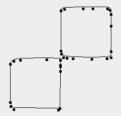
(a) $\lambda=1$

(b) $\lambda=2$

(c) $\lambda=3$

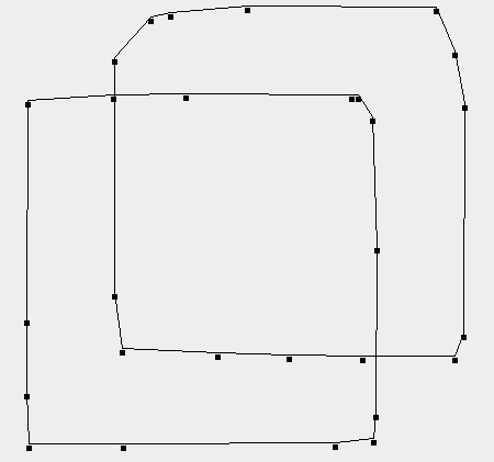
(d) $\lambda=4$

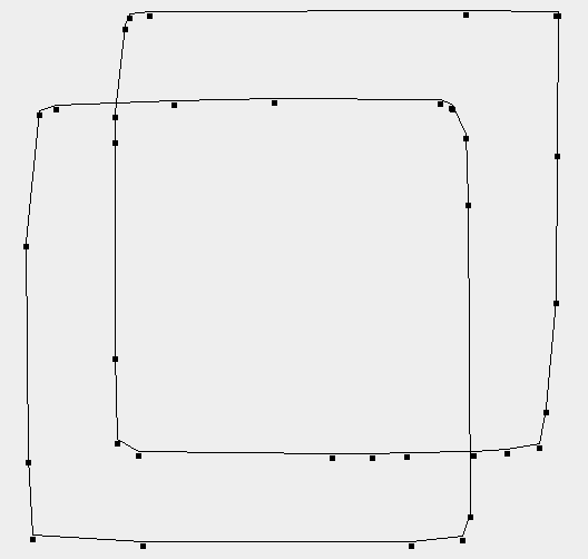
(e) $\lambda=5$

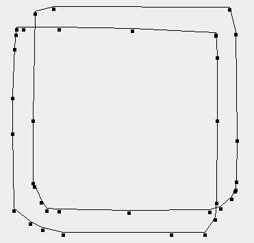
(f) $\lambda=10$

Figure 9: Example: Randomly generated 2D data with different values of $\lambda$ and $C=2$ (binary classification). Class boundaries are shown after connecting the points on convex hull for each class. While still the two classes are separable according to their boundaries, it gets harder to distinguish between the classes for larger $\lambda$ due to overlapping areas.

5.1 Parallelization for Training and Testing

We can achieve parallelization for both training and testing phases easily by partitioning according to either classes or 2DAspects. This can be done in a straight forward way following a divide and conquer approach. For instance we can partition data into different classes or partition according to indices of $(f_{1},f_{2})$ combinations. Since this is trivial, we only describe a simple divide and conquer algorithm for finding the 2D convex hull of a point set $P$, to conclude this section. It is worth to highlight that in Section 4.2, we already showed both theoretically and empirically that our convex hull algorithm reads only $O(n)$ expected number of points during its execution. Parallelization of the same algorithm using divide and conquer strategy obviously does not increase the running time. In fact, there may be no reason for parallelization in many scenarios. In cases where we want to build classifiers on demand for millions of points, it is practical to use parallelization. Algorithm 4 provides the pseudo code.

0:  Point Set $P$

0:  Convex Hull of $P$, $CH(P)$

1:  Partition $P$ into $k$ partitions $\{P_{1}...P_{k}\}$

2:  $P^{\prime}$ = empty set of points

3:  for each partition $P_{i}$ do

4:     $CH(P_{i})=$ convex hull of $P_{i}$

5:     add all the points in $CH(P_{i})$ to $P^{\prime}$

6:  $CH(P)=CH(P^{\prime})$

7:  return $CH(P)$

Algorithm 4 DivideConquerConvexHull$(P)$

We use $CH(P)$ to denote the convex hull of $P$. As described earlier, it is composed of to halves or four quarters each of which is an ordered set of points by $x$, ($f_{1}$), coordinate. The idea is simple, first we partition $P$, until the size of each $P_{i}$ is small enough. Typical running times can be estimated according to a simple cost-based analysis, and computing power/trafic available. We find the convex hull of each $P_{i}$, resulting in only a few remaining points on $CH(P_{i})$, typically constant. Having done this, we merge all $CH(P_{i})$’s. It is guaranteed that we end up with a super set of the points required for the correct answer of $CH(P)$. We find the convex hull of $P^{\prime}$ trivially in a final step.

THEOREM 3

Algorithm 4, correctly finds the convex hull of $P$, using divide and conquer.

Proof 5.1.

Proof is already explained since

$$CH(P)\subseteq\bigcup_{i=1}^{k}CH(P_{i})$$

.

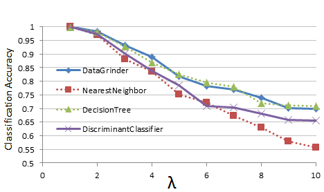
(a) Binary classification and changing $\lambda$

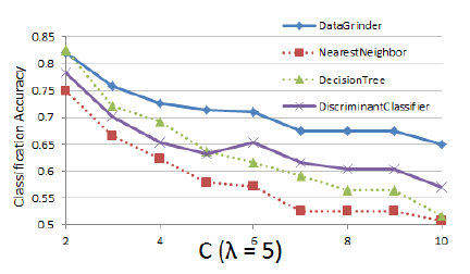
(b) Multi-class classification: fixed $\lambda$ and changing $C$

Figure 10: Classification accuracy on randomly generated datasets using $C_{i}+\lambda\times Uniform(0,1)$.

6 Experimental Analysis

We have already shown how our convex hull algorithm achieves expected $O(n)$ point reads. In this section, we already report our results regarding accuracy in different cases. First, we propose a random class generation approach, through which we can control the difficulty of the classification problem instance. We generate data only using the Uniform distribution. It is known that we can convert other distributions to Uniform as well before classification, using Normalization [39]. Here, our focus is mainly on designing DataGrinder and efficient algorithms. We report our raw results using only the algorithms described and avoid any pre/post processing to leave more room for the future work, and study the key factors involved in classification accuracy of DataGrinder, in its standard and straight forward case. We will show shortly, how DataGrinder (DGR) achieves high accuracy even in its simplest form, as described in this paper. This increases our hopes for designing highly scalable Data Mining and Machine Learning algorithms, in the Database community. Our data generation aapproach works as follows. Feature values of class $C$ (last class label), are generated as: $C+\lambda\times Uniform(0,1)$. This results in producing uniformly distributed random values for all features of class $C_{i}$, in the range $[C_{i},C_{i}+\lambda]$. For simplicity, we assume all class labels are integer, and all features are generated from the same distribution. Suppose there are only two classes, Figure 9, shows how the classification gets more complicated with increasing $\lambda$. There are two class labels $0$ and $1$. In the case of $\lambda=1$, the classes are linearly separable from each other. Therefore, any algorithm must be able to achieve $100\%$ classification accuracy, if both training and testing datasets are generated using the same $\lambda$ and $C$ parameters. As we increase $\lambda$, the two classes overlap in larger regions and thus the classification gets more complicated. We have shown our decision boundaries using convex hulls and points on them, for different values of $\lambda$ ( 9). It is also commonly known that when there are more classes (i.e. multi-class classification), the classification is more challenging. This is because we need more decision boundaries, and there is more probability for overlapping areas as well as fewer training samples for each class, compared to the number of samples from other classes. Here, we only show examples of 2D convex hulls for binary classification. As described earlier there are $2\times\binom{d}{2}$ such "2DAspects". In each case, we generate data ($X$) with 5 dimensions $f_{1},...,f_{5}$. Figure 10(a), compares DataGrinder classification accuracy, to $3$ other well-known methods for $C=2$, and changing $\lambda$. For all the other three algorithms, we use standard MATLAB functions and default parameter setting, since DataGrinder is fully non-Parametric. DecisinTree, is a text-book classifier, that achieves optimization using partitioning, information gain and obtaining a sequence of comparisons that leads to a class label with high accuracy. NearestNeighbor method searches the training dataset for a new testing instance, and assigns class label according to the closest point in the Euclidean space. DiscriminantClassifier, finds decision boundaries using $L_{1}$ and $L_{2}$ Regularization [29], in order to avoid overfitting to the training data. We train and test using $1000$ samples for training and testing each. Both Decision Tree and DiscriminantClassifier may need heavy training time if the dataset is large due to their optimization problems. Typically, at least several Sequential Scans of the dataset is the minimum required. NearestNeighbor is the most efficient, if we use space partitioning spacial indices in testing. However, the results show its accuracy is outperformed by all methods almost in all cases. Using our randomly generated data for binary classification, we find that Decision Tree and DataGrinder achieve the highest accuracy. We believe this is due to the fact that they both partition the space into regions rather than just using lines or hyperplanes as decision boundaries and our classification scenario is such that the DiscriminantClassifier fails. We fix $\lambda=5$ and repeat for multi-class classification while changing $C$. In this case, we notice all classification algorithms fail compared with DataGrinder, due to the considerable gap in accuracy. Given DataGrinder’s special scalability features for BigData, this is a bonus that DataGrinder also achieves outstanding accuracy in this experiment compared with commercial classification algorithms in MATLAB 2012.

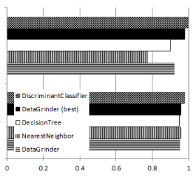
Figure 11: Classification accuracy on Wine and Iris datasets.

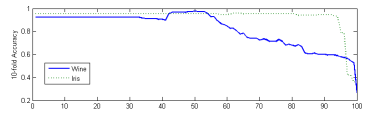
Figure 12: Using 100 "filters", for $\theta=0,0.01,0.02...1$ to find the best classifier.

6.1 Existing Classification Datasets

We use two standard datasets also used as examples in Machine Learning textbooks for the classification problem, Iris and Wine. We obtain these datasets from the UCI data mining repository . Both datasets have less than $1000$ samples and $3$ classes. We use 10-fold cross validation for training and testing, meaning we divide the dataset into $10$ partitions, and use the average of $10$ experiments. In each experiment, we use $9$ partitions for training and $1$ for testing. All algorithms reach acceptable accuracy on Iris dataset $>90\%$, and close to $1$ (Figure 11). In the case of Wine dataset, DiscriminantClassifier performs slightly superior compared to DataGrinder and DecisionTree. NearestNeighbor method is significantly outperformed by all the other algorithms. Since DiscriminantClassifier uses many parameters to achieve this, we also decide to add only $1$ hyper-parameter namely Filtering Ratio ($0\leq\theta<1$) to DataGrinder. In order to do this, we add an additional variable to each 2DAspect, Classification Accuracy. It refers to the number of training samples that correctly fall inside a 2DAspect (i.e. 2DAspect and data labels match), over the total number of all samples. Any 2DAspects that largely overlap with other classes resulting in classification accuracy less than $\theta$, are removed from DataGrinder. We vary $\theta$ using a $0.01$ step size from $0$ to $1$ over the training dataset and record the best testing accuracy. We also show in Figure 11, the best DataGrinder accuracy after filtering using a solid bar. As it is notable, DataGrinder accuracy increases after filtering, resulting in less classification errors. This also adds another dimension to our future research in order to target adding few meaningful parameters or hyper-parameter to the model that increase accuracy. The remarkable fact to highlight about the filtering technique presented is that we can achieve higher accuracy using tuning techniques and this leaves the door open for future research on DataGrinder. Figure 12, shows how DataGrinder accuracy changes on these datasets with varying $\theta$. For $\theta=0$, i.e. Raw DataGrinder, no 2DAspects are filtered. When $\theta=1$, all 2DAspects are filtered and all samples are assigned to the default class $0$. In both cases we get the best accuracy around $\theta=0.5$. This is logical, because any features whose classification rate is more than misclassification rate can be useful for discriminating between classes. When a large enough number of such features are combined, we can achieve high overall accuracy.

7 Related work

In this section, we review the recent works in literature that discuss scalable data mining algorithms and frameworks similar to DataGrinder, in motivation and technical contribution.

In [2], authors propose an "Exact Indexing" approach for Support Vector Machines. They propose indexing strategies in the Kernel space, iKernel, that is used for exact top-k query processing when SVM is used for ranking. Given a SVM model, authors use properties of the Kernel space such as ranking instability and ordering stability. They provide an excellent background of support vector machines, and their relevance to databases, top-k query processing and ranking. They only focus on prediction (i.e. testing), and do not aim at designing parallel SVM algorithms. DataGrinder, provides a highly scalable algorithmic framework for both training, model updating and testing that achieves high accuracy. We might be able to focus on future work leveraging convex hulls for constructing kernels as well as ranking. Although this requires leveraging more geometric properties of the data, in order to be able to achieve accuracy as high as Support Vector Machines. Support Vector Machine is a well researched problem with a complex structure. In contrary, DataGrinder aims at building simpler discrete models with high accuracy and our initial experimental results are promising. SVM also has applications in bioinformatics, where there are thousands of features and we need to improve DataGrinder in order to be able to deal with these applications. Biological datasets are typically more complex. Regardless of the model structure, they focus on ranking and top-k query processing while we focus on convex hulls and classification. ArrayStore [7], is a storage manager for complex array processing. Authors process datasets as big as $80GB$, using parallel data mining algorithms. They provide a multi-dimensional array model, suitable for our classification scenario. They also discuss data access issues. Our Select-Project-ConvexHull series of operations completely fits within their storage framework. Thus, we do not worry about scalability of DataGrinder at all. Rather than focus on storage, in this paper we discuss a new discrete classification algorithm, that can work on the top of ArrayStore. Authors already discuss two types of clustering algorithms, but they did not provide any examples on the classic classification problem. We provide a divide and conquer algorithm that makes DataGrinder compatible with ArrayStore. ERACER [18], provides an iterative statistical framework for filling in missing data, as well as data cleaning and fixing corrupted values using conventional statistical methods. DataGrinder can solve their problem in a special case. Extensions of DataGrinder can also solve the same exact problem. We use Computational Geometry, and theoretical analysis for a $O(n)$ expected running time algorithm while maintaining accuracy. DataGrinder can as well fit inside a DBMS engine using Select-Project-ConvexHull. We can implement ConvexHull as an operation using Table Functions. DataGrinder is fully non-Parametric, meaning that it is easy to use, and needs no parameter tuning. DataGrinder is completely discrete and we can also count on divide and conquer solutions for intense scalability. DataGrinder is easy to implement, thus suitable for the industry. DataGrinder achieves high accuracy in classification. We also show with experiments how we can improve accuracy by Filtering($\theta$). All in all, we find DataGrinder a more suitable solution for the database community, due to its strong and fundamental theoretical contributions. Spanners [12], is an interesting theoretical contribution, and a formal framework for information extraction. We believe DataGrinder has a similar flavour in its contribution to Spanners. We also aim at designing operations for processing multidimensional data and knowledge discovery. Spanners is focused on Information Extraction and using Regular Expressions for Text Mining using predefined operations. Several other previous works have also tried to achieve the same goal such as [23]. Another interesting direction to achieve parallel statistical and data mining algorithms is through Sampling [27]. In this approach, we make BigData assumption and use parallelization for processing. We build many small models and using statistical inference, we combine these models to guarantee reliability and accuracy. The size of input data and distribution(s) of data are examples of key parameters we need to take into account. Naturally, we need to focus on how to sample and pay attention to things such as the number of samples, the size of each sample as well as how to effectively combine the models built using different samplings of the data. This can be done for Big Data, regardless of the data mining task discussed. Examples of such methods include [26, 28]. Rule-based classifiers are other examples of discrete classification algorithms, discussed in the data mining literature [33, 34, 35]. They use frequent patterns and association rules mining in order to find rules with high support and confidence. They typically achieve reliable accuracy. They need a rather costly parameter tuning step to construct the best classifier. They need the exact solution of a NP-hard theoretical problem compared to $O(n)$ expected running time of DataGrinder. There have been some attempts for parallel frequent pattern mining algorithms which is outside the context of this paper.

Convex Hull problem has a long history in Computational Geometry [40]. It is significantly important, because many other important problems in Computational Geometry can be reduced to this problem. Many efforts have been devoted to improving the worst case running time and output sensitive algorithms. We find average case analysis more suitable to the database community, due to its similarity to cost-based query optimization. In [41], there is a proposal for expected $O(n)$ algorithms along with theoretical analysis to prove its possibility. In this paper, we provide an algorithm with pseudo code and calculate a exact costant, to serve as an upper-bound for the expected running time. Our experimental evaluation backs up all of our arguments, regardless of the running time and programming languages used.

8 Conclusions and Future Work

In this paper, we revisited the important problem of finding 2D convex hulls. We propose an algorithm based on a well-known historical algorithm, with $O(n)$ expected running time. We propose a simpler and shorter proof compared to the previous work, and also calculate a constant that serves as an upper-bound for the expected linear running time. We conduct experiments to back up all of our arguments. We perform several experiments and show DataGrinder is comparable to the most reliable commercial classification packages in MATLAB and outperforms many, while maintaining its extreme provable scalability. We show how to achieve several levels of parallelization, while keeping the correctness of our classification algorithm. We intend to focus on more detailed Geometrical study of the problem, in order to partition the data more accurately. Specially, remove sparse areas. We also intend to test for more classification scenarios as well as adding meaningful parameters and hyper-parameters to DataGrinder. We would also like to take DataGrinder to the cloud for classification of enormous datasets.

References

- [1] Zhang et al. Automatic Discovery of Attributes in Relational Databases. ACM SIGMOD, 2011.
- [2] Yu et al. Exact Indexing for Support Vector Machines. In ACM SIGMOD, 2011
- [3] Satuluri et al. Local Graph Sparsification for Scalable Clustering. In ACM SIGMOD, 2011.
- [4] Kohler et al. Efficient Parallel Skyline Processing using Hyperplane Projections. In ACM SIGMOD, 2011.
- [5] Agarwal et al. Latent OLAP: Data Cubes over Latent Variables In ACM SIGMOD, 2011.
- [6] Bahmani et al. Fast Personalized PageRank on MapReduce. In ACM SIGMOD, 2011.
- [7] Emad et al. ArrayStore: A Storage Manager for Complex Parallel Array Processing. In ACM SIGMOD, 2011.
- [8] Gullo et al. Advancing Data Clustering via Projective Clustering Ensembles. In ACM SIGMOD, 2011.
- [9] K. Agarwal et al. Nearest-Neighbor Searching Under Uncertainty. In PODS, 2012.
- [10] Deng et al. On the Complexity of Package Recommendation Problems. In PODS, 2012.
- [11] Kimelfeld et al. The Complexity of Mining Maximal Frequent Subgraphs. In PODS, 2013.
- [12] Fagin et al. Spanners: A Formal Framework for Information Extraction. In PODS, 2013.
- [13] Kejlberg-Rasmussen et al. I/O-Efficient Planar Range Skyline and Attrition Priority Queues. In PODS, 2013.
- [14] Chen et al. The Fine Classification of Conjunctive Queries and Parameterized Logarithmic Space Complexity. In PODS, 2013.
- [15] Jin et al. GAIA: Graph Classification Using Evolutionary Computation. In ACM SIGMOD, 2010.
- [16] Parameswaran et al. Recsplorer: Recommendation Algorithms Based on Precedence Mining. In ACM SIGMOD, 2010.
- [17] Zheng et al. K-Nearest Neighbor Search for Fuzzy Objects. ACM SIGMOD, 2010.
- [18] Mayfield et al. ERACER: A Database Approach for Statistical Inference and Data Cleaning. In ACM SIGMOD, 2010.
- [19] Gunter et al. A computational pipeline for the development of multi-marker bio-signature panels and ensemble classifiers. BMC Bioinformatics, 2012.
- [20] Ahmad et al. Predicting Completion Times of Batch Query Workloads Using Interaction-aware Models and Simulation. In EDBT, 2011.
- [21] Bilal Sheikh et al. A Bayesian Approach to Online Performance Modeling for Database Appliances using Gaussian Models. In ICAC, 2011.
- [22] Lee et al. BSkyTree: Scalable Skyline Computation Using A Balanced Pivot Selection. In EDBT, 2010.
- [23] Khabbaz et al. newblock TopRecs: Top-k Algorithms for Item-based Collaborative Filtering. newblock In EDBT, 2011.
- [24] Khabbaz et al. newblock Employing Structural and Textual Feature Extraction for Semistructured Document Classification. newblock In IEEE SMC-C, 2012.
- [25] Koochakzadeh et al. newblock Semi-Supervised Dynamic Classification for Intrusion Detection. newblock In Int. J. Soft. Eng. Knowl. Eng. 20, 2010.
- [26] Yan et al. Cluster Forests. In Computational Statistics and Data Analysis 66, 2013.
- [27] Jordan et al. Divide-and-conquer and statistical inference for big data. In ACM SIGKDD, 2012.
- [28] Jordan et al. Divide-and-Conquer Matrix Factorization. In NIPS, 2011.
- [29] Guo et al. Regularizedlinear discriminant analysis and its application in microarrays. In Biostatistics, 2007.
- [30] Koenigstein et al. Yahoo! music recommendations: modeling music ratings with temporal dynamics and item taxonomy. In ACM RecSys, 2011.
- [31] Bhagat et al. Maximizing Product Adoption in Social Networks. In, ACM WSDM, 2012.
- [32] Goyal et al. A Data-Based Approach to Social Influence Maximization. In, PVLDB, 2011.
- [33] Liu et al. Integrating classification and association rule mining. In, ACM SIGKDD, 1998.
- [34] Li et al. Accurate and efficient classification based on multiple class-association rules. In, IEEE ICDM, 2001.
- [35] Yin et al. Classification based on predictive association rules. In, SIAM SDM, 2003.
- [36] R. Agrawal et al. Fast Algorithms for Mining Association Rules in Large Databases. In, VLDB, 1994.
- [37] Han et al. Mining frequent patterns without candidate generation. In, ACM SIGMOD 2000.
- [38] Zhang et al. BIRCH: An Efficient Data Clustering Method for Very Large Databases. In, ACM SIGMOD, 1996.
- [39] C. M. Bishop. Pattern Recognition and Machine Learning. In, Springer, 2006.
- [40] Mark de Berg et al. Computational Geometry, Algorithms and Applications, Third Edition. In Springer, 2008.
- [41] Devroye et al. A Note on Linear Expected Time Algorithms for Finding Convex Hulls. In Computing, Volume 26, Issue 4, Springer, 1981.