Nonradiative and radiative Förster energy transfer between quantum dots

Abstract

We study theoretically nonradiative and radiative energy transfer between two localized quantum emitters, donor one (i.e. initially excited) and acceptor one (i.e. receiving the excitation). The rates of nonradiative and radiative processes are calculated depending on the spatial and spectral separation between donor and acceptor states and for different donor and acceptor lifetimes for typical parameters of semiconductor quantum dots. We find that the donor lifetime can be significantly modified only due to the nonradiative Förster energy transfer process at donor-acceptor separations $\sim 10$ nm (depending on the acceptor radiative lifetime) and for the energy detuning not larger than 1$\div$2 meV. The efficiency of the nonradiative Förster energy transfer process under these conditions is close to unity and decreases rapidly with the increase of donor-acceptor distance or energy detuning. At large donor-acceptor separations $>40~{}$nm the radiative corrections to the donor lifetime are comparable with nonradiative ones but are relatively weak.

I Introduction

Förster energy transfer (ET) processes are now actively studied in various fields that bridge physics, biology and chemistry. The energy is transferred from the initially excited (donor) system to the system that is initially unexcited (acceptor) via the electromagnetic interaction Förster (1948). This is an incoherent one-way transfer followed by the rapid emission or nonradiative recombination from the acceptor state that is to be distinguished from coherent light-induced coupling.Reitzenstein et al. (2006) From now on we will use the terms “donor” and “acceptor” for the energy transmitting and receiving systems. Although these terms are quite established in the literature on Förster process, they are somewhat ambiguous and should not be confused with donor and acceptor impurities in semiconductor. Here, they characterize excitation transfer and not charge transfer. The donor and acceptor systems may be realized as quantum dots,Crooker et al. (2002); Limpens et al. (2015); Liu et al. (2015); Andreakou, P. et al. (2013) quantum wires,Hernandez-Martinez et al. (2013) quantum wellsAgranovich et al. (2011); Rindermann et al. (2011) and colloidal nanoplatelets,Guzelturk et al. (2015), biological molecules,Fruhwirth et al. (2011); Galisteo-Lopez et al. (2014) defects in semiconductor.Navarro-Urrios et al. (2009); Izeddin et al. (2008) Typically, the range of the Förster interaction is on the order of several nm.Agranovich and Galanin (1982) By placing the the donors and acceptors into the structured electromagnetic environment one can try to enhance the efficiency of the transfer. In particular, the transfer, mediated by localized and surface plasmons, Pustovit and Shahbazyan (2011); Blum et al. (2012) photons trapped in the cavityAndrew and Barnes (2000) or localized in random glass,Galisteo-Lopez et al. (2014) as well as modified by metamaterialsTumkur et al. (2015); Newman et al. (2015) is now actively studied. The concept of tailored photon-induced energy transfer shares a lot of similarities with the Purcell enhancementPurcell (1946) of the spontaneous emission in the cavity as compared to that it vacuum. Indeed, in the first case one can think of nonradiative energy transfer from donor to the acceptor via (virtual) photons, while in the second case the energy is radiated into the real photonic modes (see Fig. 1). A general theory of Förster transfer process has been developed in detail.Andrews and Juzeliūnas (1992); Juzeliūnas and Andrews (1994); Dung et al. (2002); Andrews and Bradshaw (2004); Klimov et al. (2004); Allan and Delerue (2007) However, the relation between transfer process and the Purcell effect as well as the character of the transfer in each particular nanosystem, radiative or nonradiative, remains a subject of active discussions.Blum et al. (2012); Rabouw et al. (2014); Tumkur et al. (2015); Wubs and Vos (2015) Simultaneous enhancement and control of the energy transfer and spontaneous emission processes in the same electromagnetic environment are quite challenging.

Here, we study the simplest case of localized donor and acceptor (e.g. quantum dots), embedded in the dielectric matrix. We first revisit different approaches to calculate the rate of the transfer process and obtain it consistently with the donor spontaneous decay rate (Sec. II). Next, we discuss the transfer kinetics (Sec. III) and analyze the radiative and nonradiative contributions to the Förster process depending on the spatial and spectral separation of donor and acceptor as well as their intrinsic radiative lifetime (Sec. IV).

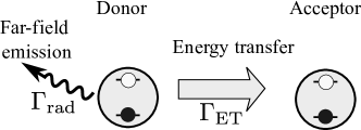
Figure 1: Schematic illustration of the energy transfer and photon radiation processes

II Calculation of the transfer rates

We consider energy transfer between two emitters in an unbounded dielectric matrix with the permittivity $\varepsilon$, located at the points $\bm{r}_{\rm D}$ (donor) and $\bm{r}_{\rm A}=\bm{r}_{\rm D}+\bm{r}$(acceptor). The relevant donor and acceptor states are characterized by the energies $E_{\rm D}=\hbar\omega_{\rm D}$ and $E_{\rm A}=\hbar\omega_{\rm A}$ and the transition dipole matrix elements $\bm{d}_{\rm D}$ and $\bm{d}_{\rm A}$. In the following we neglect the dispersion and losses in the matrix. We first present the Fermi Golden rule result for the transfer rate (Sec. II.1) and then compare it with the semiclassical Langevin approach (Sec. II.2).

II.1 Fermi Golden rule

The Fermi Golden rule yields the following expression for the transfer rate

$$\Gamma_{\rm ET,0}=\frac{2\pi}{\hbar}\delta(E_{\rm D}-E_{\rm A})|\bm{d}_{\rm D}\hat{G}_{0}\bm{d}_{\rm A}|^{2}\>,$$ (1)

where

$$G_{0,\alpha\beta}=\frac{3r_{\alpha}r_{\beta}-r^{2}\delta_{\alpha\beta}}{\varepsilon r^{5}}$$ (2)

is the electromagnetic Green function evaluated in the electrostatic approximation, and describing the dipole-dipole coupling between donor and acceptor.Agranovich and Galanin (1982) This result can be applied for quantum dots as well as molecules. For quantum dots, we have neglected the local field corrections for the electric fieldde Vries et al. (1998); Poddubny (2015a) assuming the permittivities of the dot and the matrix to be the same. In the case of spherical dots these corrections lead to renormalization of the dipole matrix element, $\bm{d}_{\rm D,A}\to\bm{d}_{\rm D,A}3\varepsilon_{\rm QD}/(\varepsilon_{\rm QD}+2\varepsilon)$, where $\varepsilon_{\rm QD}$ is the dot permittivity. In the general case one has to introduce the depolarization factors depending on the dot orientation and shape. Additional local field corrections appear for dense arrays of quantum dots. Poddubny (2015a); Pukhov et al. (2008)

The result Eq. (1) scales with the distance as $1/r^{6}$. However, Eq. (1) neglects any effects of retardation for the electromagnetic interaction. When the retardation effects are taken into account, the transfer rate can be still presented in the form Eq. (1), but the electrostatic potential Eq. (2) should be replaced by the full retarded electromagnetic Green tensor Dung et al. (2002)

$$G_{\alpha\beta}=\left(\delta_{\alpha\beta}+\frac{1}{q^{2}}\frac{\partial^{2}}{\partial x_{\alpha}\partial x_{\beta}}\right)\frac{e^{{\rm i}qr}}{\varepsilon r}$$ (3)

evaluated at the transition frequency $\omega=E_{\rm D}/\hbar\equiv E_{\rm A}/\hbar$, where $q=\omega_{\rm D}\sqrt{\varepsilon}/c$, so that

$$\Gamma_{\rm ET}=\frac{2\pi}{\hbar}\delta(E_{\rm D}-E_{\rm A})|\bm{d}_{\rm D}\hat{G}\bm{d}_{\rm A}|^{2}\>.$$ (4)

In this case the long-range radiative transfer, that scales with the distance as $1/r^{2}$, becomes possible.Agranovich and Galanin (1982) The explicit values for the matrix elements of the interaction $g=\bm{d}_{\rm D}\hat{G}_{0}\bm{d}_{\rm A}$ in the cases, when the dipole momenta of donor and acceptor are parallel to each other and either parallel or perpendicular to the vector $\bm{r}=\bm{r}_{\rm D}-\bm{r}_{\rm A}$ read

$$g_{\parallel}=d_{\rm A}d_{\rm D}\frac{{\rm e}^{{\rm i}qr}}{\varepsilon}\left(\frac{2}{r^{3}}-\frac{2{\rm i}q}{r^{2}}\right)\>,$$ (5)

$$g_{\perp}=d_{\rm A}d_{\rm D}\frac{{\rm e}^{{\rm i}qr}}{\varepsilon}\left(-\frac{1}{r^{3}}+\frac{{\rm i}q}{r^{2}}+\frac{q^{2}}{r}\right)\>.$$

For random mutual orientation of the donor and acceptor matrix elements the transfer is described by the value $|g^{2}|=(1/3)|g_{\parallel}^{2}|+(2/3)|g_{\perp}^{2}|$, averaged over the orientations.

II.2 Semiclassical approach

Here, we are going to re-derive Eq. (1) within the Langevin random source technique and the semiclassical theory of light-matter interaction.Ivchenko (2005); Vogel and Welsch (2006); Deych et al. (2007)

II.2.1 Radiative decay of the donor

We start with the radiative decay of the donor state in the absence of acceptors. The donor electric polarizability tensor reads

$$\alpha_{\mu\nu}(E)=\frac{d_{D,\mu}d_{D,\nu}}{E_{\rm D}-E},$$ (6)

i.e. its dipole moment $\bm{p}_{\rm D}$ induced by the external electric field $\bm{E}$ at the frequency $\hbar\omega$ is given by

$$\bm{p}_{\rm D}=\frac{\bm{d}_{\rm D}\bigl{[}\bm{d}_{\rm D}\cdot\bm{E}(\bm{r}_{\rm D})\bigr{]}}{E_{\rm D}-\hbar\omega}\>.$$ (7)

On the another hand, the electric field of the donor is determined by the Green function Eq. (3) ,

$$\bm{E}(\bm{r})=\hat{G}(\bm{r}-\bm{r}_{\rm D})\bm{p}_{\rm D}\>.$$ (8)

Combining Eq. (7) and Eq. (8) we obtain the self-consistency condition for the mode of donor coupled with its own electromagnetic field:

$$(E_{\rm D}-\hbar\omega)\bm{p}_{\rm D}=\bm{d}_{\rm D}[\bm{d}_{\rm D}\cdot\hat{G}(0,\omega)\bm{p}_{\rm D}]\>.$$ (9)

This equation allows one to determine the modification of the lifetime of the donor state due to the interaction with light. The energy shift of the donor state can be obtained as well, but this requires regularization of the Green function taking the finite extent of the wave function into account, see Refs. Ivchenko, 2005; de Vries et al., 1998. Below we assume, that such regularization has been already performed and is included in the definition of the energy $E_{\rm D}$. We also use the weak coupling approximation when the Green function in the right-hand side of Eq. (9) is evaluated at the frequency $\omega_{\rm D}$. The spontaneous emission rate is then determined from Eq. (9) as

$$\Gamma_{\rm rad,0}\equiv-2\mathop{\mathrm{missing}}{Im}\nolimits\omega=2d_{\rm D,\alpha}\mathop{\mathrm{missing}}{Im}\nolimits\hat{G}_{\alpha\beta}(0,\omega_{\rm D})d_{\rm D,\beta},$$ (10)

or, explicitly,Novotny and Hecht (2006)

$$\Gamma_{\rm rad,0}=\frac{4d_{D}^{2}}{3\hbar}\left(\frac{\omega_{\rm D}}{c}\right)^{3}\sqrt{\varepsilon}\>.$$ (11)

II.2.2 Donor decay in the presence of acceptor

Equation (11) is a textbook result for the spontaneous emission rate.Novotny and Hecht (2006) However, the approach above can be straightforwardly generalized to include the energy transfer processes.Pustovit et al. (2013); Poddubny (2015b) To this end, Eqs. (8)–(9) should be modified to account for the electromagnetic coupling of the donor and the acceptor as follows:

$$(\omega_{\rm D}-\omega)\bm{p}_{\rm D}=\frac{1}{\hbar}\bm{d}_{\rm D}[\bm{d}_{\rm D}\cdot(\hat{G}(0,\omega)\bm{p}_{\rm D})+\hat{G}(\bm{r},\omega)\bm{p}_{\rm A}]\>,$$ (12)

$$(\omega_{\rm A}-{\rm i}\gamma_{\rm A}-\omega)\bm{p}_{\rm A}=\frac{1}{\hbar}\bm{d}_{\rm A}[\bm{d}_{\rm A}\cdot\hat{G}(\bm{r},\omega)\bm{p}_{\rm D}]\>.$$

Here, we include the phenomenological (nonradiative) decay rate $\gamma_{\rm A}$ for the acceptor excited state. The decay is due to the energy relaxation to the lower acceptor states. We are interested in the weak coupling regime, and consider the energy relaxation of the acceptor state to be much faster than the energy transfer and the radiative decay of both donor and acceptor states. Hence, the donor lifetime in the presence of acceptor is given by the perturbative solution of the system Eqs. (12) at the frequency close to $\omega_{\rm D}$. The result can be presented as

$$\frac{1}{\tau_{{\rm D},0}}=\Gamma_{{\rm rad},0}\,,\quad\frac{1}{\tau_{\rm D}}=\Gamma_{{\rm rad},0}+\Gamma_{\rm D},$$ (13)

$$\Gamma_{\rm D}=\frac{2}{\hbar}\mathop{\mathrm{missing}}{Im}\nolimits\left[\frac{1}{\omega_{\rm A}-{\rm i}\gamma_{\rm A}-\omega_{\rm D}}\frac{1}{\hbar^{2}}\left(\bm{d}_{\rm D}\cdot\hat{G}(\bm{r})\bm{d}_{\rm A}\right)^{2}\right]\>.$$ (14)

The second term in Eq. (13) describes the acceptor-induced contribution to the decay rate of the donor state. This expression is quite different from the standard result Eq. (4). First, Eq. (14) includes the finite lifetime of the acceptor state. Second, the functional dependence of Eq. (4) and Eq. (14) on the (complex) Green function is different. The difference between Eq. (4) and Eq. (14) constitutes the central result of this work. Qualitatively, it is due to the fact that Eq. (4) describes only the rate of the generation of particles in the acceptor state. On the other hand, Eq. (14) is the total acceptor-induced modification of the donor decay rate, which is contributed by both energy transfer to the acceptor and modification of the spontaneous decay rate. In the following Sec. IV we will analyze Eq. (4) and Eq. (14) in more detail. Here, we only mention that in the case when the distance between the donor and the acceptor becomes much smaller than the wavelength, $qr\ll 1$ and the retardation effects are neglected, Eq. (14) reduces to

$$\Gamma_{D,0}=\frac{2\pi}{\hbar}\frac{1}{\pi\hbar}\frac{\gamma_{\rm A}}{(\omega_{\rm D}-\omega_{\rm A})^{2}+\gamma_{\rm A}^{2}}|\bm{d}_{\rm D}\hat{G}_{0}\bm{d}_{\rm A}|^{2}.$$ (15)

This expression is equivalent to the Fermi Golden rule result Eq. (1) in the limit of the vanishing acceptor decay rate. Here we consider only the case of transparent medium, $\mathop{\mathrm{missing}}{Im}\nolimits\varepsilon=0$. The more general case of lossy medium, where the additional decay channel due to medium heating is possible, has been analyzed in Ref. Barnett et al., 1996, see also Ref. Glazov et al., 2011.

II.2.3 Population of acceptors

In the previous paragraph we have calculated the decay rates of donor state. Now we will obtain the acceptor population using the same semiclassical technique. To this end, we consider the regime of stationary incoherent pumping and use the random source approach.Deych et al. (2007) Hence, the system Eq. (12) is modified as

$$(\omega_{\rm D}-\omega)\bm{p}_{\rm D}=\frac{1}{\hbar}\bm{d}_{\rm D}[\bm{d}_{\rm D}\cdot(\hat{G}(0,\omega)\bm{p}_{\rm D}) +\hat{G}(\bm{r},\omega)\bm{p}_{\rm A}]$$

$$\qquad+\bm{d}_{\rm D}\xi(\omega)\>,$$

$$(\omega_{\rm A}-{\rm i}\gamma_{\rm A}-\omega)\bm{p}_{\rm A}=\frac{1}{\hbar}\bm{d}_{\rm A}[\bm{d}_{\rm A}\cdot\hat{G}(\bm{r},\omega) \bm{p}_{\rm D}]\>,$$ (16)

where $\xi(\omega)$ is the random source term describing the stationary incoherent generation of excitons in the donor state. Generally, the correlations of the random sources are determined by the pumping mechanism,Averkiev et al. (2009) the simplest approximation corresponds to white Gaussian noise

$$\langle\xi^{*}(\omega)\xi(\omega^{\prime})\rangle=\frac{S}{2\pi}\delta(\omega-\omega^{\prime}),\quad\langle\xi^{*}(t)\xi(t^{\prime})\rangle=S\delta(t-t^{\prime})$$ (17)

where $S$ is the exciton generation rate. First, we calculate the stationary donor state population as

$$N_{\rm D}=\frac{\langle|\bm{p}_{\rm D}(t)|^{2}\rangle}{|\bm{d}_{\rm D}|^{2}},$$ (18)

where

$$\bm{p}_{\rm D}(t)=\int\frac{{\rm d}\omega}{2\pi}\bm{p}_{\rm D}(\omega){\rm e}^{-{\rm i}\omega t}\>.$$ (19)

and the angular brackets denote the averaging over the random source realizations. Explicitly, we obtain

$$N_{\rm D}=\left\langle\left|\int\frac{{\rm d}\omega}{2\pi}\mathcal{D}_{\rm D}(\omega)\xi(\omega){\rm e}^{-{\rm i}\omega t}\right|^{2}\right\rangle,$$ (20)

where

$$\mathcal{D}_{\rm D}(\omega)=\frac{1}{\omega_{\rm D}-\omega-{\rm i}/(2\tau_{\rm D})}$$ (21)

is the donor Green function calculated including both energy transfer and radiative decay processes. The averaging and integration yields $N_{\rm D}=S\tau_{\rm D}\>,$ i.e. the donor population is equal to the product of the lifetime and the generation rate. The acceptor population is obtained in a similar way as

$$N_{\rm A}\equiv\frac{\langle|\bm{p}_{\rm A}|^{2}\rangle}{|\bm{d}_{\rm A}|^{2}}=S|\bm{d}_{\rm D}\cdot\hat{G}_{0}\bm{d}_{\rm A}|^{2}\int\frac{{\rm d}\omega}{2\pi}|\mathcal{D}_{\rm A}(\omega)|^{2}|\mathcal{D}_{\rm D}(\omega)|^{2}$$ (22)

with

$$\mathcal{D}_{\rm A}(\omega)=\frac{1}{\omega_{\rm A}-\omega-{\rm i}\gamma_{\rm A}}\>.$$ (23)

The result of integration reads

$$N_{\rm A}=\frac{2\pi}{\hbar}S\tau_{\rm D}\tau_{\rm A}\frac{1}{\pi\hbar}\frac{\gamma_{\rm A}}{(\omega_{\rm A}-\omega_{\rm D})^{2}+\gamma_{\rm A}^{2}}|\bm{d}_{\rm D}\hat{G}_{0}\bm{d}_{\rm A}|^{2}\>,$$ (24)

where $\tau_{\rm A}=1/(2\gamma_{\rm A})$. It is instructive to rewrite this result in the form of the kinetic equation for balance of the (nonradiative) decay in the acceptor state and the energy transfer from the donors

$$\frac{N_{\rm A}}{\tau_{\rm A}}=\Gamma_{\rm ET}N_{\rm D}\>.$$ (25)

Using this equation as the definition of the energy transfer rate $\Gamma_{\rm ET}$, we find from Eq. (24)

$$\Gamma_{\rm ET}=\frac{2\pi}{\hbar}\Theta|\bm{d}_{\rm D}\cdot\hat{G}\bm{d}_{\rm A}|^{2},\quad\Theta=\frac{1}{\pi\hbar}\frac{\gamma_{\rm A}}{(\omega_{\rm A}-\omega_{\rm D})^{2}+\gamma_{\rm A}^{2}}\>$$ (26)

which is the generalization of Eq. (4) to the case of finite acceptor state lifetime. Eq. (26) directly corresponds to the expression commonly used for the realistic multilevel systems,Crooker et al. (2002); Liu et al. (2015) [e.g. Eq. (1) from Ref. Liu et al., 2015] with $\Theta$ being the overlap integral between the donor emission and the acceptor absorption spectra for the considered model with two-level donor and acceptor. We note, that these results can be equivalently obtained using the Keldysh diagram technique,Keldysh (1965) its correspondence to the Langevin source technique for this problem is discussed in Refs. Deych et al., 2007; Averkiev et al., 2009.

II.3 Ohmic losses approach

The acceptor excitation rate Eq. (26) can be also calculated in a slightly different but equivalent way as the rate of the absorption of donor emission.Pustovit and Shahbazyan (2011); Agranovich et al. (2011) This allows one to interpret the energy transfer process in the form of the Ohmic losses for the donor emission. Thus, one can separate the contributions to the total donor decay rate Eq. (14), determined by the energy transfer process and by the modification of the far-field emission by the acceptor.

In particular, the acceptor dipole moment induced by the donor with the dipole moment $\bm{p}_{D}=\bm{d}_{D}$ is obtained from the second of Eqs. (12) as

$$p_{A,\alpha}=\frac{d_{A,\alpha}d_{A,\beta}G_{\beta\gamma}d_{D,\gamma}}{\hbar(\omega_{\rm A}-\omega_{\rm D}-{\rm i}\gamma_{\rm A})}\>,$$ (27)

and the electric field at the acceptor position is given by

$$E_{\alpha}(\bm{r}_{\rm A})=G_{\alpha\beta^{\prime}}(\bm{r})d_{D,\beta^{\prime}}\>.$$ (28)

The rate of power absorption is then determined by the standard electrodynamic expressionLandau and Lifshitz (1974)

$$\frac{1}{\tau_{\rm ET}}\equiv\Gamma_{\rm ET}=2\mathop{\mathrm{missing}}{Im}\nolimits p_{A,\alpha}E^{*}_{D,\alpha}.$$ (29)

Substituting Eq. (27) and Eq. (28) into Eq. (29) we recover Eq. (26).

In order to distinguish between the energy transfer and the far-field emission processes we will use the identityVogel and Welsch (2006)

$$\int{\rm d}^{3}r^{\prime\prime}G_{\mu\nu}(\bm{r},\bm{r}^{\prime\prime})G^{*}_{\mu^{\prime}\nu}(\bm{r}^{\prime},\bm{r}^{\prime\prime})\varepsilon^{\prime\prime}(\bm{r}^{\prime\prime})=4\pi\mathop{\mathrm{missing}}{Im}\nolimits G_{\mu\mu^{\prime}}(\bm{r},\bm{r}^{\prime})\>.$$ (30)

valid for the Green function in arbitrary medium in the case of zero external stationary magnetic field. For $\bm{r}=\bm{r}^{\prime}$ the right-hand side determines the local density of photonic states and the radiative decay rate.Sprik et al. (1996) For $\mu=\nu^{\prime},\bm{r}=\bm{r}^{\prime}$ Eq. (30) simplifies to

$$\mathop{\mathrm{missing}}{Im}\nolimits\int{\rm d}^{3}r^{\prime\prime}\frac{\varepsilon(\bm{r}^{\prime\prime})-1}{4\pi}|G^{*}_{\mu^{\prime}\nu}(\bm{r}^{\prime\prime},\bm{r})|^{2}=\mathop{\mathrm{missing}}{Im}\nolimits G_{\mu\mu}(\bm{r},\bm{r})\>.$$ (31)

The radiative decay rate is due to the far-field emission and due to the Joule heating of the medium. The Joule losses are determined as the integral in the left hand side over the finite volume, where $\mathop{\mathrm{missing}}{Im}\nolimits\varepsilon\neq 0$. The far-field emission is given from the contribution to the integral at $r^{\prime\prime}\to\infty$ for $\mathop{\mathrm{missing}}{Im}\nolimits\varepsilon(\bm{r}^{\prime\prime})\to 0$. For given $\mu$ the integral can be rewritten as $\mathop{\mathrm{missing}}{Im}\nolimits\int d^{3}r^{\prime\prime}\bm{\Pi}(\bm{r}^{\prime\prime})\bm{E}^{*}(\bm{r}^{\prime\prime})$, where $\Pi$ is the polarizability tensor,

$$\Pi_{\beta}(\bm{r}^{\prime\prime})=\frac{\varepsilon(\bm{r}^{\prime\prime})-1}{4\pi}G_{\beta\alpha}(\bm{r}^{\prime\prime},\bm{r}),\quad E_{\beta}(\bm{r}^{\prime\prime})=G_{\beta\alpha}(\bm{r}^{\prime\prime},\bm{r})\>.$$ (32)

This expression is equivalent to Eq. (29) and corresponds to the transfer rate $\Gamma_{\rm ET}$ in Eq. (26). The total acceptor-induced decay rate of the donor state $\Gamma_{\rm D}$ in Eq. (14) includes the contribution Eq. (26) due to the Ohmic losses and the correction to the far-field emission. Thus, the far-field contribution is obtained as the difference between $\Gamma_{\rm D}$ and $\Gamma_{\rm ET}$,

$$\Delta\Gamma_{\rm rad}=\Gamma_{\rm D}-\Gamma_{\rm ET}\>.$$ (33)

III Kinetic equations

In the previous section we have presented four approaches yielding consistent results, namely (i) Fermi Golden rule to calculate the transfer rate to the acceptor state Eq. (1) neglecting the losses and retardation, (ii) coupled dipole technique to calculate the donor decay rate Eq. (14), (iii) random sources technique and (iv) Joule power losses approach to calculate the transfer rate for the acceptor state Eq. (26).

These results allow us to formulate the following system of phenomenological kinetic equations determining the population of the donor and acceptor states $N_{\rm D}$ and $N_{\rm A}$, and the population $N_{{\rm A},0}$ of the acceptor ground (emitting) state which lifetime $\tau_{{\rm A},0}$ is controlled by the spontaneous emission:

$$\frac{{\rm d}N_{\rm D}}{{\rm d}t} =-\left(\Gamma_{\rm rad,0}+\Delta\Gamma_{\rm rad}\right)N_{\rm D}-\Gamma_{\rm ET}N_{\rm D}+S$$

$$\equiv-\frac{N_{\rm D}}{\tau_{\rm D}}+S\>,$$

$$\frac{{\rm d}N_{\rm A}}{{\rm d}t} =-\frac{N_{\rm A}}{\tau_{\rm A}}+\Gamma_{\rm ET}N_{\rm D}\>,$$

$$\frac{{\rm d}N_{{\rm A},0}}{{\rm d}t} =-\frac{N_{{\rm A},0}}{\tau_{{\rm A},0}}+\frac{N_{\rm A}}{\tau_{\rm A}}\>.$$ (34)

Here, $S$ is the exciton generation rate for the donor state, and the total acceptor-induced correction to the donor decay rate $\Gamma_{\rm D}=\Gamma_{\rm ET}+\Delta\Gamma_{\rm rad}$ consists of two parts, the correction due to acceptor excitation ($\Gamma_{\rm ET}$ ) and the correction corresponding to the far field emission ($\Delta\Gamma_{\rm rad}$). In the case of small distance between donor and acceptor the value of $g$ is almost real, $\Gamma_{\rm D}=\Gamma_{\rm A}$ and $\Gamma_{\rm rad}\ll\Gamma_{\rm D}$. The expression for $\Gamma_{\rm rad}$ can be explicitly written as

$$\Delta\Gamma_{\rm rad}=-\frac{4}{\hbar}\frac{2(\mathop{\mathrm{missing}}{Im}\nolimits g)^{2}\gamma_{\rm A}+2\Delta\mathop{\mathrm{missing}}{Im}\nolimits(g)\mathop{\mathrm{missing}}{Re}\nolimits g}{\Delta^{2}+\gamma_{\rm A}^{2}}\>,$$ (35)

where $g=\bm{d}_{D}\cdot\hat{G}\bm{d}_{A}$ and $\Delta=\omega_{\rm D}-\omega_{\rm A}$. Hence, $\Delta\Gamma_{\rm rad}$ is not equal to zero only when the retardation effects are taken into account ($\mathop{\mathrm{missing}}{Im}\nolimits g\neq 0$). This means that the term $\Delta\Gamma_{\rm rad}$ corresponds to the radiation of real photons. On the other hand, $\Gamma_{\rm ET}$ is proportional to $(\mathop{\mathrm{missing}}{Re}\nolimits g)^{2}+(\mathop{\mathrm{missing}}{Im}\nolimits g)^{2}$, i.e. it includes contributions of both real and virtual photons.Andrews and Bradshaw (2004)

In the general case the values of $\Delta\Gamma_{\rm rad}$ and $\Gamma_{\rm D}$ can be negative. For vanishing detuning between donor and acceptor ($\Delta=0$) one has $|\Gamma_{\rm D}|<\Gamma_{\rm ET}$, and $\Delta\Gamma_{\rm rad}<0$, i.e. the far field emission is suppressed, see Eq. (35). For large detuning, ($|\Delta|\gg\gamma_{\rm A}$) the value of $\Gamma_{\rm\rm rad}$ can be positive, i.e. the far field emission is enhanced. It is also possible, that $\Gamma_{\rm D}$ is equal to zero, but $\Gamma_{\rm ET}$ is not zero. This means that the growth of the donor decay rate due to transfer is exactly compensated by the suppression of the far field emission from the donor.

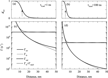
Figure 2: Distance dependence of the energy transfer for $\Delta=0$ and $\tau_{\rm rad,0}\approx 1~{}$ns (a,c) and $\tau_{\rm rad,0}\approx 100~{}$ns (b,d). Panels (a) and (b) show the transfer efficiency $K_{\rm ET}$, panels (c) and (d) show the full donor decay rates $\Gamma_{\rm D}$ (thin solid curves), energy transfer rates $\Gamma_{\rm ET}$ (thick solid curves), radiative decay rates $\Gamma_{\rm rad}$ (dotted curves) and the full donor decay rate $\Gamma_{\rm D}+\Gamma_{\rm rad,0}$ (dashed curves). Other calculation parameters are as follows: $\tau_{A}=1~{}$ps, $\Delta=0$, $E_{\rm D}=2~{}$eV, $d_{D}=d_{A}=e\times 0.32$ nm (a,c), $d_{D}=d_{A}=e\times 0.032$ nm (b,d) , $\varepsilon_{b}=10$. The rates are averaged over donor and acceptor orientations. Arrows in (a), (b) indicate the Förster radii where $K_{\rm ET}=0.5$.

We stress that in our model the lifetime of the acceptor excited state $\tau_{\rm A}$ is determined by the nonradiative process and is the shortest time in the system, while the lifetime of the acceptor ground state $\tau_{{\rm A},0}$ is of the same order as $\tau_{{\rm D},0}$ so that $\tau_{\rm A}\ll\tau_{{\rm A},0}\approx\tau_{{\rm D},0}$. As discussed above, the donor lifetime $\tau_{{\rm D}}$ can be shortened or lengthened in the presence of acceptor, however the condition $\tau_{\rm A}\ll\tau_{{\rm D}}$ remains valid.

The dynamics of the system Eq. (24) in the absence of stationary pumping for given population of donors at $t=0$ under these conditions is given by

$$N_{\rm D} = N_{\rm D}(0){\rm e}^{-t/\tau_{\rm D}},$$ (36)

$$N_{\rm A} = \Gamma_{\rm ET}N_{\rm D}(0)\frac{\tau_{\rm A}\tau_{\rm D}}{\tau_{\rm A}-\tau_{\rm D}}({\rm e}^{-t/\tau_{\rm A}}-{\rm e}^{-t/\tau_{\rm D}})$$

$$\approx \Gamma_{\rm ET}N_{\rm D}(0)\tau_{\rm A}{\rm e}^{-t/\tau_{\rm D}}\,,$$

$$N_{{\rm A},0} = \Gamma_{\rm ET}N_{\rm D}(0)\frac{\tau_{{\rm A},0}\tau_{\rm D}}{\tau_{{\rm A},0}-\tau_{\rm D}}\left({\rm e}^{-t/\tau_{{\rm A},0}}-{\rm e}^{-t/\tau_{\rm D}}\right)\,.$$

For stationary pumping the solution of Eqs. (24) reads

$$N_{\rm D}=G\tau_{\rm D},\quad N_{\rm A}=\Gamma_{\rm ET}\tau_{\rm A}N_{\rm D},\quad N_{{\rm A},0}=\Gamma_{\rm ET}\tau_{\rm A,0}N_{\rm D}.$$ (37)

The acceptor population in the ground (emitting) state can be also rewritten as

$$N_{{\rm A},0}=G\tau_{A,0}K_{\rm ET}\>,$$ (38)

where

$$K_{\rm ET}=\frac{\Gamma_{\rm ET}}{1/\tau_{\rm D,0}+\Gamma_{\rm D}}=\frac{\Gamma_{\rm ET}\tau_{\rm D,0}}{1+\Gamma_{\rm D}\tau_{\rm D,0}}\>$$ (39)

is the efficiency of the energy transfer. If we assume that the quantum yield of donor emission without acceptor was equal to one and its intensity was just given by $I_{\rm D}=G$, the modified donor intensity in the presence of acceptor is now given by $I_{\rm D}^{*}=G(1-K_{\rm ET})$, while the intensity from acceptor is given by $I_{\rm A}^{*}=GK_{\rm ET}$. It turns out that in the presence of FRET with $\Gamma_{\rm ET}>0$ the quantum efficiency of the donor PL is always decreased even in the case $\Delta\Gamma_{\rm rad}>0$ (increase of the donor radiative rate). However, the increase of the donor radiative rate decreases the efficiency of the energy transfer and vice versa without changing the energy transfer rate $\Gamma_{\rm ET}$.

Figure 3: Dependence of the energy transfer efficiency $K_{\rm ET}$ on the radiative rate $\Gamma_{\rm rad,0}$ for different donor-acceptor distances $r$ . Calculation has been performed for $\Delta=0$ and the same other parameters as in Fig. 2.

Figure 4: Dependence of the energy transfer efficiency $K_{\rm ET}$ on the donor-acceptor energy detuning $\Delta$ for $\tau_{\rm rad,0}=1~{}$ns (a) and $\tau_{\rm rad,0}=100~{}$ns (b). Thick solid, dotted, thin solid, and dashed curves correspond to donor-acceptor distance $r=13$ nm, $8~{}$nm, 6 nm and 4 nm, respectively. Other calculation parameters are the same as in Fig. 2.

IV Results and discussion

Now we proceed to the analysis of the transfer efficiency and transfer rates. We study their dependence on the donor-acceptor distance $r$ (Fig. 2), radiative lifetimes $\tau_{\rm rad,0}$ (Fig. 3) and spectral detunings $\Delta$ (Fig. 4). Figure 2 examines the distance dependence of the efficiency $K_{\rm ET}$ (a,b) and the rates $\Gamma_{\rm ET}$, $\Gamma_{\rm D}$, $\Gamma_{\rm rad}$, $\Gamma_{\rm D}+\Gamma_{\rm rad,0}$ (c,d). We have chosen two respresentative values of the dipole matrix elements $d_{\rm D}=d_{\rm A}$, resulting in the bare radiative lifetimes $\tau_{\rm rad,0}=1$ ns (Fig. 2a,Fig. 2c) and $\tau_{\rm rad,0}=100$ ns (Fig. 2b,Fig. 2d). The typical values of the radiative decay times for the bright exciton in quantum dots may vary from 0.2–0.3 ns to 20 ns depending on the dot type,Biadala et al. (2014); Patton et al. (2003) while for the dark quantum dot exciton transitions the times may vary from 100 ns to 1–2 $\mu$s.Liu et al. (2015); Patton et al. (2003) It has been recently demonstrated that at low temperatures dark excitons determine the energy transfer in dense ensemble of colloidal CdTe nanocrystals.Liu et al. (2015) The nonradiative decay rate of the acceptor state $\tau_{\rm A}$ is equal to $1$ ps.Klimov et al. (2000) For short radiative lifetime $\tau_{\rm rad,0}=1$ ns the transfer is efficient ($K_{\rm ET}>0.5$) up to the distance $r\approx 13$ nm, which is by definition the radius of the Förster process. For larger radius $\Gamma_{\rm ET}$ becomes smaller than $\Gamma_{\rm rad}$ (cf. solid and dotted curves in Fig. 2c) and the transfer is suppressed. Comparing thick and thin solid curves in panel (c) one can see, that up to $r\lesssim 40$ nm one has $\Gamma_{\rm ET}\approx\Gamma_{\rm D}$. This means that the transfer is purely nonradiative for $r\lesssim 40$ nm. At larger distances, when the curves deviate, the radiative correction becomes comparable with the transfer rate, although still smaller than $\Gamma_{\rm rad}$. However, at such large distances the transfer is quite inefficient, $K_{\rm ET}\ll 1$. Thus, we conclude from the analysis of Fig. 2a and Fig. 2c that when the Förster process is efficient, it is nonradiative. For longer radiative lifetime $\tau_{\rm rad,0}=100$ ns (Fig. 2b and Fig. 2d) the distance dependence of the transfer remains qualitatively the same, but the Förster radius shrinks to about $6$ nm. The sensitivity of the Förster radius to the radiative lifetime reflects the fact that the radiative rate $\Gamma_{\rm rad,0}$ and the Förster rate $\Gamma_{\rm ET}$ are proportional to the second and fourth power of the dipole matrix element, respectively. In Fig. 2 the dipole matrix element has been chosen equal for donors and acceptors, $d_{D}=d_{A}$, so its increase boosts the relative efficiency of the transfer. Hence, in order to enhance Förster interaction between the quantum states of the same origin it is beneficial to select the acceptor states with radiative lifetime that is short (but still longer than the nonradiative time $\tau_{A}$). The dependence of the Förster radius on the radiative lifetime is further analyzed in Fig. 3. It shows the transfer efficiencies at different donor acceptor distances as functions of the radiative rate. The calculation confirms that the transfer at the distances beyond $10$ nm requires the radiative lifetime of the acceptor excited state to be as short as 1 ns.

Finally, in Fig. 4 we present the dependence of the transfer efficiency $K_{\rm ET}$ on the energy detuning between donor and acceptor $\Delta$ for different distances $r=13$ nm, $8~{}$nm, $6$ nm, and $4$ nm (thick solid, dotted, thin solid, and dashed curves, respectively) and for two different radiative lifetimes $\tau_{\rm rad,0}=1$ ns (a) and $\tau_{\rm rad,0}=100$ ns (c). The transfer efficiency is a Lorentzian function of the detuning with maximum at $\Delta=0$. For $\tau_{\rm rad,0}=1$ ns (a) the spectral range of the transfer is on the order of meV and increases at smaller donor-acceptor distances. For long radiative lifetime $\tau_{\rm rad,0}=100$ ns the spectral range strongly decreases and the transfer becomes possible only for the detuning less than $1~{}$meV and donor-acceptor distance $r\lesssim 5$ nm. The detuning range allowing for the transfer is also inversely proportional to the nonradiative lifetime of the acceptor state $\tau_{A}=1/2\gamma_{A}$, directly entering the overlap integral $\Theta$ in Eq. (26).

V Summary

To summarize, we have presented a theory of the Förster interaction, accounting both for the transfer of the energy from the donor to the acceptor (Förster effect) and for the antenna-like modification of the far-field donor emission by the acceptor (Purcell effect). We have demonstrated for typical parameters corresponding to the semiconductor quantum dots that the Purcell effect is negligible provided that the transfer efficiency is high, $K_{\rm ET}>0.5$. In another words, the fast transfer is purely nonradiative. The radiative corrections start to play role only at relatively large distances $r>40$ nm when the transfer is quenched. We have analyzed the dependence of the Förster radius on the radiative lifetime and revealed that the radius above 10 nm can be achieved only utilizing bright donor and acceptor excitonic states with the radiative lifetime on the order of $1~{}$ns. In this case the transfer takes place provided that the detuning between donor and acceptor does not exceed several meV.

While our theory is quite general, it should be stressed that the numerical results above are applicable only to the transfer in the homogeneous dielectric matrix. The competition between radiative and nonradiative transfer mechanisms in the case of structured electromagnetic environment (plasmonicTumkur et al. (2015); Newman et al. (2015) or dielectricWubs and Vos (2015)) requires further studies.

References

- Förster (1948) T. Förster, Annalen der Physik 437, 55 (1948).
- Reitzenstein et al. (2006) S. Reitzenstein, A. Löffler, C. Hofmann, A. Kubanek, M. Kamp, J. P. Reithmaier, A. Forchel, V. D. Kulakovskii, L. V. Keldysh, I. V. Ponomarev, et al., Opt. Lett. 31, 1738 (2006).
- Crooker et al. (2002) S. Crooker, J. Hollingsworth, S. Tretiak, and V. Klimov, Phys. Rev. Lett. 89, 186802 (2002).
- Limpens et al. (2015) R. Limpens, A. Lesage, P. Stallinga, A. N. Poddubny, M. Fujii, and T. Gregorkiewicz, J. Phys. Chem. C 119, 19565 (2015).
- Liu et al. (2015) F. Liu, A. V. Rodina, D. R. Yakovlev, A. A. Golovatenko, A. Greilich, E. D. Vakhtin, A. Susha, A. L. Rogach, Y. G. Kusrayev, and M. Bayer, Phys. Rev. B 92, 125403 (2015).
- Andreakou, P. et al. (2013) Andreakou, P., Brossard, M., Li, C., Lagoudakis, P. G., Bernechea, M., and Konstantatos, G., EPJ Web of Conferences 54, 01017 (2013).
- Hernandez-Martinez et al. (2013) P. L. Hernandez-Martinez, A. O. Govorov, and H. V. Demir, J. Phys. Chem. C 117, 10203 (2013).
- Agranovich et al. (2011) V. M. Agranovich, Y. N. Gartstein, and M. Litinskaya, Chem. Rev. 111, 5179 (2011).
- Rindermann et al. (2011) J. J. Rindermann, G. Pozina, B. Monemar, L. Hultman, H. Amano, and P. G. Lagoudakis, Phys. Rev. Lett. 107, 236805 (2011).
- Guzelturk et al. (2015) B. Guzelturk, M. Olutas, S. Delikanli, Y. Kelestemur, O. Erdem, and H. V. Demir, Nanoscale 7, 2545 (2015).
- Fruhwirth et al. (2011) G. O. Fruhwirth, L. P. Fernandes, G. Weitsman, G. Patel, M. Kelleher, K. Lawler, A. Brock, S. P. Poland, D. R. Matthews, G. Kéri, et al., ChemPhysChem 12, 442 (2011).
- Galisteo-Lopez et al. (2014) J. F. Galisteo-Lopez, M. Ibisate, and C. Lopez, J. Phys. Chem. C 118, 9665 (2014).
- Navarro-Urrios et al. (2009) D. Navarro-Urrios, A. Pitanti, N. Daldosso, F. Gourbilleau, R. Rizk, B. Garrido, and L. Pavesi, Phys. Rev. B 79, 193312 (pages 4) (2009).
- Izeddin et al. (2008) I. Izeddin, D. Timmerman, T. Gregorkiewicz, A. S. Moskalenko, A. A. Prokofiev, I. N. Yassievich, and M. Fujii, Phys. Rev. B 78, 035327 (2008).
- Agranovich and Galanin (1982) V. M. Agranovich and M. Galanin, Electronic excitation energy transfer in condensed matter (North-Holland Pub. Co., Amsterdam, 1982).
- Pustovit and Shahbazyan (2011) V. N. Pustovit and T. V. Shahbazyan, Phys. Rev. B 83, 085427 (2011).
- Blum et al. (2012) C. Blum, N. Zijlstra, A. Lagendijk, M. Wubs, A. P. Mosk, V. Subramaniam, and W. L. Vos, Phys. Rev. Lett. 109, 203601 (2012).
- Andrew and Barnes (2000) P. Andrew and W. L. Barnes, Science 290, 785 (2000).
- Tumkur et al. (2015) T. U. Tumkur, J. K. Kitur, C. E. Bonner, A. N. Poddubny, E. E. Narimanov, and M. A. Noginov, Faraday Discuss. 178, 395 (2015).
- Newman et al. (2015) W. Newman, C. Cortes, D. Purschke, A. Afshar, Z. Chen, G. De los Reyes, F. Hegmann, K. Cadien, R. Fedosejevs, and Z. Jacob, in Lasers and Electro-Optics (CLEO), 2015 Conference on (2015), pp. 1–2.
- Purcell (1946) E. M. Purcell, Phys. Rev. 69, 681 (1946).
- Andrews and Juzeliūnas (1992) D. L. Andrews and G. Juzeliūnas, J. Chem. Phys. 96, 6606 (1992).
- Juzeliūnas and Andrews (1994) G. Juzeliūnas and D. L. Andrews, Phys. Rev. B 49, 8751 (1994).
- Dung et al. (2002) H. T. Dung, L. Knöll, and D.-G. Welsch, Phys. Rev. A 65, 043813 (2002).
- Andrews and Bradshaw (2004) D. L. Andrews and D. S. Bradshaw, European J. Physics 25, 845 (2004).
- Klimov et al. (2004) V. Klimov, S. K. Sekatskii, and G. Dietler, J. Modern Optics 51, 1919 (2004).
- Allan and Delerue (2007) G. Allan and C. Delerue, Phys. Rev. B 75, 195311 (2007).
- Rabouw et al. (2014) F. T. Rabouw, S. A. den Hartog, T. Senden, and A. Meijerink, Nature Communications 5, 3610 (2014).
- Wubs and Vos (2015) M. Wubs and W. L. Vos, ArXiv e-prints (2015), eprint 1507.06212.
- de Vries et al. (1998) P. de Vries, D. V. van Coevorden, and A. Lagendijk, Rev. Mod. Phys. 70, 447 (1998).
- Poddubny (2015a) A. N. Poddubny, J. Optics 17, 035102 (2015a).
- Pukhov et al. (2008) K. K. Pukhov, T. T. Basiev, and Y. V. Orlovskii, JETP Lett. 88, 12 (2008).
- Ivchenko (2005) E. L. Ivchenko, Optical Spectroscopy of Semiconductor Nanostructures (Alpha Science International, Harrow, UK, 2005).
- Vogel and Welsch (2006) W. Vogel and D.-G. Welsch, Quantum Optics (Wiley, Weinheim, 2006).
- Deych et al. (2007) L. I. Deych, M. V. Erementchouk, A. A. Lisyansky, E. L. Ivchenko, and M. M. Voronov, Phys. Rev. B 76, 075350 (2007).
- Novotny and Hecht (2006) L. Novotny and B. Hecht, Principles of Nano-Optics (Cambridge University Press, New York, 2006).
- Pustovit et al. (2013) V. N. Pustovit, A. M. Urbas, and T. V. Shahbazyan, Phys. Rev. B 88, 245427 (2013).
- Poddubny (2015b) A. N. Poddubny, Phys. Rev. B 92, 155418 (2015b).
- Barnett et al. (1996) S. M. Barnett, B. Huttner, R. Loudon, and R. Matloob, J. Phys. B 29, 3763 (1996).
- Glazov et al. (2011) M. Glazov, E. Ivchenko, A. Poddubny, and G. Khitrova, Phys. Solid State 53, 1753 (2011).
- Averkiev et al. (2009) N. S. Averkiev, M. M. Glazov, and A. N. Poddubnyi, JETP 108, 836 (2009).
- Keldysh (1965) L. V. Keldysh, Sov. JETP Lett. 20, 1018 (1965).
- Landau and Lifshitz (1974) L. Landau and E. Lifshitz, Electrodynamics of Continuous Media (Pergamon, New York, 1974).
- Sprik et al. (1996) R. Sprik, B. A. van Tiggelen, and A. Lagendijk, Europhys. Lett. 35, 265 (1996).
- Biadala et al. (2014) L. Biadala, F. Liu, M. D. Tessier, D. R. Yakovlev, B. Dubertret, and M. Bayer, Nano Lett. 14, 1134 (2014).
- Patton et al. (2003) B. Patton, W. Langbein, and U. Woggon, Phys. Rev. B 68, 125316 (2003).
- Klimov et al. (2000) V. I. Klimov, A. A. Mikhailovsky, D. W. McBranch, C. A. Leatherdale, and M. G. Bawendi, Science 287, 1011 (2000).