Exchangeability, the ‘Histogram Theorem’,
and population inference

Abstract

Some practical results are derived for population inference based on a sample, under the two qualitative conditions of ‘ignorability’ and exchangeability. These are the ‘Histogram Theorem’, for predicting the outcome of a non-sampled member of the population, and its application to inference about the population, both without and with groups. There are discussions of parametric versus non-parametric models, and different approaches to marginalisation. An Appendix gives a self-contained proof of the Representation Theorem for finite exchangeable sequences.

Keywords: sampling, surveys, prediction, Finite Representation Theorem

1   Introduction

This paper concerns the relationship between the histogram of a sample and proportions in the underlying population. Our intuition is that these two distinct objects must be similar, but cannot be identical. As a simple illustration, we would not automatically assign a population proportion of zero to a label which was not present in the sample histogram. The purpose of this paper is to derive and publicize some practical results: the ‘Histogram Theorem’ (Theorem 1 in section 2), and its implications for sample-based population inference, eqs (13) and (15).

Any quantitative assessment of the relationship between the sample histogram and the population must depend on a statistical model of the sampling procedure. I will assume that the sampling process is ‘ignorable’, as described in Gelman et al., (2014, ch. 8). On the basis of ‘ignorability’ alone, it is possible to make inferences about the population using ‘design-based’ estimation, e.g. as discussed in Little, (2004), Brewer, (2002), and Brewer and Gregoire, (2009). I will adopt what is often characterised as a competing mode of inference, which is to include an explicit statistical model for the population. Brewer and Gregoire, (2009) term this ‘prediction-based’ estimation, although ‘model-based’ is also common.

My statistical model for the population is that it is exchangeable in the quantities of interest, either in toto or within identifiable groups. A set of random quantities is exchangeable exactly when beliefs (probabilities) about any subset are the same as beliefs about any other subset of the same size; see section 2 for the formal definition. I prefer to regard exchangeability as a ‘boundary condition’. To say “I am treating my beliefs about the population as exchangeable” asserts that I am choosing to ignore everything about the population except for the values that are collected in the sample. Where exchangeability is confined within groups, the assertion is that I am choosing to ignore everything about the population except its group structure and the values that are collected in the sample. It is often expedient to make such an assertion; in some circumstances it is also equitable. On this interpretation, the restrictions implied by the exchangeable model are to be welcomed, rather than seen as ‘unrealistic’.

The key result in the paper is the ‘Histogram Theorem’, stated and proved in section 2. This result relates the predictive probability distribution of an unsampled member of the population to the histogram of the sample, in terms of an upper bound on the total variation distance. Its practical implications are discussed in section 3. Population inference is described in section 4, which improves the folk theorem that the sample histogram predicts the population proportions. This result is extended to a more limited form of exchangeability (within but not between groups). Section 5 discusses the role of parametric population models, and clarifies the meaning of ‘non-parametric’ in the context of exchangeable beliefs. Section 6 considers the effect of merging labels, which happens implicitly whenever a multiple-question survey is analysed marginally, one question at a time. A self-contained Appendix states and proves the Finite Representation Theorem for exchangeable random quantities (Theorem 2), providing more details for some of the steps in the main text.

2   Prediction in finite exchangeable sequences

Let $\boldsymbol{X}\mathrel{:=}\nolinebreak(X_{1},\dots,X_{m})$ be a finite sequence of random quantities, where each $X_{i}$ has the same finite realm

$$\mathcal{X}\mathrel{:=}\nolinebreak\left\{\vphantom{\big{(}}x^{(1)},\dots,x^{(k)}\right\}.$$

The finite $k$ does not exclude the case where the the realm of the $X$’s is non-finite. In this case the set $\mathcal{X}$ represents a specified finite partition of the realm of $X_{i}$, and may thus have additional topological structure. But I will not assume any such structure in what follows, and hence I will treat the $x^{(j)}$ simply as ‘labels’.

In this paper $\boldsymbol{X}$ is an exchangeable sequence, which is to say that

$$\operatorname{E}\{g(X_{1},\dots,X_{m})\}=\operatorname{E}\{g(X_{\pi_{1}},\dots,X_{\pi_{m}})\}$$ (1)

for any real-valued function $g$ and any permutation $(\pi_{1},\dots,\pi_{m})$. See Schervish, (1995, ch. 1), Kingman, (1978), or Aldous, (1985) for results and insights about exchangeable sequences, and Diaconis, (1977) and Diaconis and Freedman, (1980) for the special case of finite exchangeability, as used here. An Appendix at the end of the paper provides the necessary details about exchangeability, including a statement and proof of the Finite Representation Theorem (Theorem 2).

An equivalent statement for exchangeable $\boldsymbol{X}$ with finite realms is that the probability mass function (PMF) depends only on the histogram of $\boldsymbol{x}$, denoted

$$\boldsymbol{h}(\boldsymbol{x})\mathrel{:=}\nolinebreak\big{(}h_{1}(\boldsymbol{x}),\dots,h_{k}(\boldsymbol{x})\big{)},$$

where $h_{j}(\boldsymbol{x})$ is the number of elements of $\boldsymbol{x}$ with label $x^{(j)}$. Thus the PMF for $\boldsymbol{X}$ can be expressed as

$$f_{\boldsymbol{X}}(\boldsymbol{x})=f_{\boldsymbol{H}}^{m}\{\boldsymbol{h}(\boldsymbol{x})\}\big{/}\,\mathcal{M}_{\boldsymbol{h}(\boldsymbol{x})}$$ (2)

where $f_{\boldsymbol{H}}^{m}$ is a PMF for histograms of $m$ elements allocated over $k$ labels, and $\mathcal{M}_{\boldsymbol{h}(\boldsymbol{x})}$ is the Multinomial coefficient, defined in (A4), which represents the number of distinct sequences $\boldsymbol{x}$ which have the same histogram $\boldsymbol{h}(\boldsymbol{x})$.

If $\boldsymbol{X}$ is an exchangeable sequence then any subsequence of $\boldsymbol{X}$ is also an exchangeable sequence (this is obvious from eq. 1). Without loss of generality, I will focus on the subsequence comprising the first $n+1$ elements of $\boldsymbol{X}$, denoted $(\boldsymbol{X}_{1:n},X_{n+1})$. The predictive distribution of $X_{n+1}$ given $\boldsymbol{x}_{1:n}$ is denoted

$$f^{*}_{j}\mathrel{:=}\nolinebreak\operatorname{Pr}\{X_{n+1}\mathrel{\dot{=}}\nolinebreak x^{(j)}\mathbin{|}\nolinebreak\boldsymbol{X}_{1:n}\mathrel{\dot{=}}\nolinebreak\boldsymbol{x}_{1:n}\}\qquad j=1,\dots,k,$$ (3)

to be derived below; I prefer to use dots to indicate binary predicates in infix notation. This predictive distribution has an exact expression originating from $f_{\boldsymbol{H}}^{m}$, although this expression will typically be very complicated (see the Appendix).

One intuitive approximation to $f^{*}_{j}$ is

$$\tilde{f}_{j}\mathrel{:=}\nolinebreak\frac{h_{j}+1}{n+k}\qquad j=1,\dots,k,$$ (4)

where from now on I will suppress the ‘$(\boldsymbol{x}_{1:n})$’ argument on $\boldsymbol{h}(\boldsymbol{x}_{1:n})$ and $h_{j}(\boldsymbol{x}_{1:n})$, to save clutter. In other words, add one to each count in the histogram and normalise the result. In Machine Learning this is sometimes termed ‘add one smoothing’ (see, e.g., Murphy,, 2012, p. 79). Obviously (4) is a very attractive approximation, if it is accurate, because it makes no reference to $f_{\boldsymbol{H}}^{m}$, and is trivial to compute. The first objective of this paper is to prove the following result, on the basis of which I refer to (4) as the ‘HT approximation’. I write $\boldsymbol{h}\oplus j$ to denote the histogram $\boldsymbol{h}$ with $1$ added to the count of the $j$th label.

Theorem 1 (Histogram Theorem).

Let $\beta$ satisfy

$$1+\beta=\frac{\vphantom{\big{(}}\max_{j}f_{\boldsymbol{H}}^{n+1}(\boldsymbol{h}\oplus j)}{\vphantom{\big{(}}\min_{j^{\prime}}f_{\boldsymbol{H}}^{n+1}(\boldsymbol{h}\oplus j^{\prime})}.$$

Then the total variation distance between $(f^{*}_{1},\dots,f^{*}_{k})$ and $(\tilde{f}_{1},\dots,\tilde{f}_{k})$ is no greater than $\tfrac{1}{2}\,\beta$.

Note that the Histogram Theorem is a pure exchangeability result which requires no additional structure; e.g. no super-populations or parameters, as used in Ericson, (1969). Parameters will be discussed further in section 5. An operational interpretation of the Histogram Theorem is given at the start of section 3.

The proof comes in two parts. First, I derive an exact expression for $f^{*}_{j}$, then I derive the total variation bound. For the first part, I generalise the approach of David Blackwell, in his discussion of Diaconis, (1988). The marginal distribution of $\boldsymbol{X}_{1:n}$ can be derived from $f_{\boldsymbol{X}}$ given in (2); denote it as

$$f_{\boldsymbol{X}_{1:n}}(\boldsymbol{x}_{1:n})=f_{\boldsymbol{H}}^{n}(\boldsymbol{h})\big{/}\,\mathcal{M}_{\boldsymbol{h}},$$ (5)

where $f_{\boldsymbol{H}}^{n}(\boldsymbol{h})$ is deduced from $f_{\boldsymbol{H}}^{m}$; this is the necessary form because$\boldsymbol{X}_{1:n}$ is exchangeable (see the Appendix). The predictive distribution has its standard quotient form:

$$f^{*}_{j}=\frac{f_{\boldsymbol{X}_{1:n},X_{n+1}}(\boldsymbol{x}_{1:n},x^{(j)})}{f_{\boldsymbol{X}_{1:n}}(\boldsymbol{x}_{1:n})}$$ (6)

where we can assume that the denominator is non-zero (otherwise $f_{\boldsymbol{H}}^{m}$ would need to be revised in the light of the sample). Write

$$r_{j}\mathrel{:=}\nolinebreak\frac{f^{*}_{j}}{f^{*}_{1}}\quad\text{so that}\quad f^{*}_{j}=\frac{r_{j}}{\sum_{j^{\prime}}r_{j^{\prime}}}.$$ (7)

Now evaluate $r_{j}$ in terms of (5) and (6) to give

$$r_{j}=\frac{\vphantom{\big{(}}f_{\boldsymbol{H}}^{n+1}(\boldsymbol{h}\oplus j)\big{/}\,\mathcal{M}_{\boldsymbol{h}\oplus j}}{\vphantom{\big{(}}f_{\boldsymbol{H}}^{n+1}(\boldsymbol{h}\oplus 1)\big{/}\,\mathcal{M}_{\boldsymbol{h}\oplus 1}}=\frac{\vphantom{\big{(}}f_{\boldsymbol{H}}^{n+1}(\boldsymbol{h}\oplus j)}{\vphantom{\big{(}}f_{\boldsymbol{H}}^{n+1}(\boldsymbol{h}\oplus 1)}\cdot\frac{h_{j}+1}{h_{1}+1}\mathrel{=:}\nolinebreak u_{j}\cdot v_{j}\,,$$ (8)

say, introducing the terms $u_{j}$ and $v_{j}$. In these terms,

$$f^{*}_{j}=\frac{u_{j}\,v_{j}}{\sum_{j}u_{j^{\prime}}\,v_{j^{\prime}}}\quad\text{and}\quad\tilde{f}_{j}=\frac{v_{j}}{\sum_{j^{\prime}}v_{j^{\prime}}}$$ (9)

from (7) and (4), respectively. From now on I write

$$\boldsymbol{\tilde{f}}\mathrel{:=}\nolinebreak\big{(}\tilde{f}_{1},\dots,\tilde{f}_{k}\big{)},$$

and similarly for $\boldsymbol{f^{*}}$ above, $\boldsymbol{\hat{f}}$ and $\boldsymbol{{\hat{f}^{\prime}}}$ in section 3, and $\boldsymbol{\tilde{p}}$ and $\boldsymbol{\tilde{p}}_{g}$ in section 4.

The second part of the proof consists of showing under what conditions the $u$’s in (9) can be ignored, allowing $\boldsymbol{\tilde{f}}$ to be a good approximation to $\boldsymbol{f^{*}}$. Here I co-opt the more general result of L.J. Savage in Edwards et al., (1963), his ‘Principle of stable estimation’. In Savage’s notation, my condition in the Histogram Theorem reads

$$\varphi\leq u_{j}\leq(1+\beta)\,\varphi$$

for every $u_{j}$, where in my case $\varphi\mathrel{:=}\nolinebreak\min_{j}u_{j}$. It follows immediately that

$$\varphi\sum\nolimits_{j}v_{j}\leq\sum\nolimits_{j}u_{j}\,v_{j}\leq(1+\beta)\,\varphi\sum\nolimits_{j}v_{j}$$ (10)

and, with only a little more work, that

$$\frac{1}{1+\beta}\leq\frac{f^{*}_{j}}{\tilde{f}_{j}}\leq 1+\beta\qquad j=1,\dots,k,$$ (11)

from (9) and (10). Then, for the total variation distance,

$$\big{\|}\boldsymbol{f^{*}}-\boldsymbol{\tilde{f}}\big{\|}_{\text{TV}} \mathrel{:=}\nolinebreak\sup_{C\subset\mathcal{X}}\left\lvert\vphantom{\big{(}}f^{*}(C)-\tilde{f}(C)\right\rvert$$

$$=\frac{1}{2}\sum\nolimits_{j}\left\lvert\vphantom{\big{(}}f^{*}_{j}-\tilde{f}_{j}\right\rvert \mathcal{X}$$ as is finite

$$=\frac{1}{2}\sum\nolimits_{j}\left\lvert\frac{f^{*}_{j}}{\tilde{f}_{j}}-1\right\rvert\tilde{f}_{j} \tilde{f}_{j}>0$$ as

$$\leq\frac{1}{2}\sum\nolimits_{j}\max\left\{\frac{\beta}{1+\beta},\beta\right\}\tilde{f}_{j}$$ from (11)

$$=\frac{1}{2}\,\beta$$

as was to be shown. This completes the proof of the Histogram Theorem.

Savage provided a more general result than the version used here, with conditions on the $v$’s as well as the $u$’s, that might be useful in establishing a tighter upper bound if the histogram is highly concentrated in a subset of the labels.

Michael Goldstein (pers. comm.) has provided me with a simple illustration of when $\beta$ is infinite: the case where you are sure that all the $X$’s take the same value, but unsure of what that value is. In this case the histogram $\boldsymbol{h}$ will have all $n$ cases with the same label, and one of the ‘add one’ histograms adjacent to $\boldsymbol{h}$ will be consistent with this, while the other $k-1$ will not. Hence $\beta$ is of the form $1/0$, and $\big{\|}\boldsymbol{f^{*}}-\boldsymbol{\tilde{f}}\big{\|}_{\text{TV}}$ takes its maximum value of $1$. But in this case a sample larger than one is not required (except for caution), and exact predictions are straightforward.

3   Some simple implications

The Histogram Theorem (HT) suggests the following procedure for making a prediction about an unobserved $X_{i}$, based on a sample taken from a population treated as exchangeable. First, contemplate the sample histogram $\boldsymbol{h}$. If you have no strong beliefs about the ‘add one’ histograms adjacent to $\boldsymbol{h}$, in the sense that you do not believe that the most probable of them, a priori, is much more probable than the least probable, then your $\beta$ in the HT is small, and the HT approximation in (4) gives an accurate prediction. This procedure is illustrated in Figure 1.

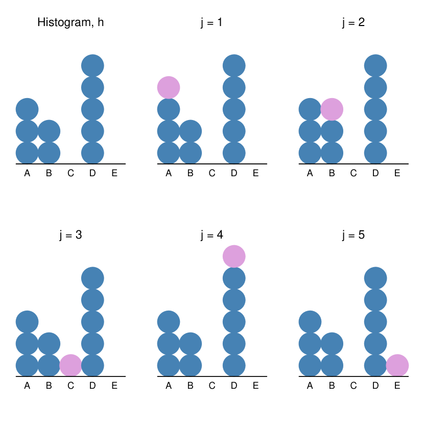
Figure 1: Contemplating the histogram $\boldsymbol{h}$ in order to reflect on the size of $\beta$. In this illustration, $k=5$, $n=10$, and $\boldsymbol{h}=(3,2,0,5,0)$. The five ‘add one’ histograms adjacent to $\boldsymbol{h}$ are constructed, and the value of $\beta$ is inferred from the ratio of the probabilities of the the most probable to the least probable, a priori, for an exchangeable population of size $m$ (not explicitly specified here).

You may be comfortable with the qualitative assessment of $\beta$ as ‘small’. But if, after contemplation of $\boldsymbol{h}$, you are prepared to quantify $\beta$ as, say, ‘not larger than $0.2$’, then you can be sure, from the upper bound on the total variation distance, that none of your HT-approximation predictions can be off by more than $10$ percentage points from your true prediction. This might be accurate enough for your purposes. Heuristically at least, you might conclude that $\left\lvert\vphantom{\big{(}}f^{*}_{j}-\tilde{f}_{j}\right\rvert\ll 0.1$ for each $j$, on the grounds that it would be unlikely for the entire error of the HT approximation to concentrate on a single label.

Note the overtly subjective nature of the HT approximation, which depends on your assessment of your $\beta$. Exchangeability constrains the PMF $f_{\boldsymbol{X}}$, but only to within an uncountably infinite set of candidates (see section 5 and the Appendix). Your particular $f_{\boldsymbol{X}}$ from this set might imply a very large $\beta$, as in the example at the end of the previous section. But, of course, if you actually had a particular $f_{\boldsymbol{X}}$ you would not need an approximation. So the HT serves those analysts, presumably the vast majority, who have qualitative beliefs about $\boldsymbol{X}$, which might well emerge into sharper focus when tested with specific questions. Contemplating $\boldsymbol{h}$ and asking “How big is my $\beta$?” is one such question. To accept that your $\beta$ is not larger than $0.2$ implicitly narrows your $f_{\boldsymbol{X}}$ to a subset of all possible exchangeable PMFs, without requiring you to be more specific.

We can also turn the HT around, to use the contrapositive. If, knowing the HT, you choose not to use the HT approximation then you must believe that at least one of the ‘add one’ histograms adjacent to $\boldsymbol{h}$ is much more probable, a priori, than another. So it turns out in this case that you have strong beliefs about $\boldsymbol{X}$: your rejection of the HT approximation has revealed this to you, even if you did not know it beforehand.

If you do not like $\boldsymbol{\tilde{f}}$ as an approximation to your $\boldsymbol{f^{*}}$, then perhaps this is because $\boldsymbol{\tilde{f}}$ is flatter than you would like. It is certainly flatter than the ‘maximum likelihood’ (ML) approximation

$$\hat{f}_{j}\mathrel{:=}\nolinebreak\frac{h_{j}}{n}\qquad j=1,\dots,k.$$

This is obvious from writing $\boldsymbol{\tilde{f}}$ as the shrinkage estimator

$$\boldsymbol{\tilde{f}}=\frac{n}{n+k}\,\boldsymbol{\hat{f}}+\frac{k}{n+k}\,(k^{-1}\boldsymbol{1})$$

where $\boldsymbol{1}$ is the vector of $k$ ones. It is straightforward to show that

$$\big{\|}\boldsymbol{\tilde{f}}-\boldsymbol{\hat{f}}\big{\|}_{\text{TV}}=\frac{k}{n+k}\,\big{\|}\boldsymbol{\hat{f}}-(k^{-1}\boldsymbol{1})\big{\|}_{\text{TV}}.$$ (12)

Therefore a necessary condition for preferring the more concentrated $\boldsymbol{\hat{f}}$ to $\boldsymbol{\tilde{f}}$ is that $n$ is not large relative to $k$, otherwise there would be no appreciable difference between the two PMFs. I will define an ‘under-powered’ study as one where $n$ is not large relative to $k$; say, for concreteness, that $n$ is not at least $9k$. So, to put the condition differently, perhaps more starkly, you can only find yourself in the position of preferring the ML approximation to the HT approximation if you have performed an under-powered study.

Limited resources often constrain us to perform under-powered studies. Suppose you find yourself, in such a study, preferring the ML approximation to the HT approximation. According to the established norms of science (see, e.g., Ziman,, 2000, ch. 3), you must be careful to ensure that your preference is rooted in an assessment of the accuracy of the two approximations, rather than in the personal approval that derives from presenting a more concentrated prediction.

One possibility for such an assessment is to modify the proof of the HT to derive an upper bound on $\big{\|}\boldsymbol{f^{*}}-\boldsymbol{\hat{f}}\big{\|}_{\text{TV}}$. But there is a technical difficulty, which is that $h_{j}=0$ would involve a division by zero, and a trivial upper bound of $1$. So consider a slightly modified ML approximation

$${\hat{f}^{\prime}}_{j}\mathrel{:=}\nolinebreak\frac{h_{j}\vee 1}{n+v}\qquad j=1,\dots,k$$

where ‘$\vee$’ denotes the pairwise maximum, and $v$ is the number of labels for which $h_{j}=0$. Then it is straightforward to adapt the proof of the HT to give $\big{\|}\boldsymbol{f^{*}}-\boldsymbol{{\hat{f}^{\prime}}}\big{\|}_{\text{TV}}\leq\tfrac{1}{2}\gamma$, where

$$\gamma\mathrel{:=}\nolinebreak\frac{\max_{j}f_{\boldsymbol{H}}^{n+1}(\boldsymbol{h}\oplus j)\cdot(h_{j}+1)/(h_{j}\vee 1)}{\min_{j^{\prime}}f_{\boldsymbol{H}}^{n+1}(\boldsymbol{h}\oplus j^{\prime})\cdot(h_{j^{\prime}}+1)/(h_{j^{\prime}}\vee 1)}.$$

Unfortunately this bound does not lend itself to a simple assessment procedure. Unlike for $\beta$, it is no longer simply a case of comparing histograms, which might be done semi-qualitatively, but, instead, of attaching a probability to each histogram in order to make a quantitative adjustment based on $\boldsymbol{h}$. However, a simple upper bound on $\gamma$ can be found using the smallest and largest values of $\boldsymbol{h}$, denoted $\underline{h}$ and $\overline{h}$ respectively:

$$\gamma\leq\beta\,\frac{(\underline{h}+1)/(\underline{h}\vee 1)}{(\overline{h}+1)/\overline{h}}.$$

But since this upper bound is larger than $\beta$, and likely to be a lot larger, it cannot serve the purpose of justifying the choice of the ML approximation over the HT approximation. So, to continue the stark theme from the previous paragraph, it is hard to make the case that the ML approximation is better than the HT approximation, in under-powered studies where they differ. From this I conclude that, in the absence of strong beliefs for which $\beta$ is large, we should prefer the HT approximation to the ML approximation.

4   Population inference

Usually, the sample of size $n$ is collected to make an inference about the population of size $m$. For example, the Mayor would like to know the proportion of the electorate who are ‘very happy’ with his incumbency, measured on a Likert scale of $1$ (very unhappy) to $5$ (very happy). Budgetary and time restrictions often limit the size of the sample, such that the sample fraction $n/m$ is small.

4.1 Point prediction

For a point prediction I will use the conditional expectation; i.e. the Bayes estimate under quadratic loss (Ghosh and Meeden,, 1997, section 1.3, adopt a similar approach to population prediction). Denote the target random quantity of interest as

$$P_{j}\mathrel{:=}\nolinebreak\frac{1}{m}\sum_{i=1}^{m}\mathds{1}_{X_{i}\mathrel{\dot{=}}\nolinebreak x^{(j)}}\qquad j=1,\dots,k,$$

the proportion of the population with label $j$. Taking expectations,

$$\begin{split}\operatorname{E}^{*}(P_{j})&=\frac{1}{m}\left(h_{j}+\sum_{i=n+1}^{m}\operatorname{Pr}^{*}(X_{i}\mathrel{\dot{=}}\nolinebreak x^{(j)})\right)\\[1.07639pt] &=\left(\frac{n}{m}\right)\hat{f}_{j}+\left(1-\frac{n}{m}\right)f^{*}_{j}\\[3.22916pt] &\approx\left(\frac{n}{m}\right)\hat{f}_{j}+\left(1-\frac{n}{m}\right)\tilde{f}_{j}\mathrel{=:}\nolinebreak\tilde{p}_{j}\qquad j=1,\dots,k,\end{split}$$ (13)

using an asterisk to indicate conditioning on $\boldsymbol{X}_{1:n}\mathrel{\dot{=}}\nolinebreak\boldsymbol{x}_{1:n}$, as before. The approximation in the final line uses the HT to replace $\boldsymbol{f^{*}}$ by $\boldsymbol{\tilde{f}}$, on the condition that $\beta$ is small. This approximation can easily be adapted to predictions of functions of $\boldsymbol{X}$, for example in applications where $\mathcal{X}$ is a set of numbers or vectors.

Eq. (13) shows that the prediction $\boldsymbol{\tilde{p}}$ is a weighted average of the ML approximation and the HT approximation, where the weight is the sample fraction $n/m$. As was discussed in section 3, in under-powered studies it is possible that $\boldsymbol{\tilde{f}}\not\approx\boldsymbol{\hat{f}}$, and the case was made there that we should prefer $\boldsymbol{\tilde{f}}$ to $\boldsymbol{\hat{f}}$ as an approximation to $\boldsymbol{f^{*}}$. Thus, if the sample fraction is very small, then the approximate prediction for small $\beta$ should be $\boldsymbol{\tilde{p}}\approx\boldsymbol{\tilde{f}}$ and not $\boldsymbol{\tilde{p}}\approx\boldsymbol{\hat{f}}$.

To be absolutely clear, the barchart displaying $\boldsymbol{\tilde{p}}$ should be titled ‘Prediction based on a survey of size $n$’, and the vertical axis should be labelled ‘Proportion of the electorate’. By way of contrast, the sample bar chart should be titled ‘Survey of size $n$’, and the vertical axis should be labelled ‘Number’. This distinction should alert other analysts to the different meanings of the two possibly similar but definitely not identical-looking figures.

4.2 Inference involving groups

Often the population can be divided into distinct groups, where each member belongs to exactly one group. For example, the electorate can be divided into men and women, or divided over the product of several factors, such as sex, age, and ethnicity. Another possibility is to stratify the population according to the binned values of one or more continuous values.

Where there are groups, it is natural to implement exchangeability within groups but not across groups, as discussed in Lindley and Novick, (1981). This need not involve any additional statistical modelling under an additional condition, given immediately below in (14).

Let there be $s$ groups indexed by $g$, so that the random quantity of interest is

$$P_{j}=\sum_{g=1}^{s}\frac{m_{g}}{m}P_{gj}\qquad j=1,\dots,k,$$

where $m_{g}$ is the size of group $g$ (taken as known, at least approximately), and $P_{gj}$ is the proportion of group $g$ which has label $j$. The crucial simplifying assumption is that the samples are sufficiently large, and the groups sufficiently distinct, that

$$\operatorname{E}^{*}(P_{gj})\approx\operatorname{E}(P_{gj}\mathbin{|}\nolinebreak\boldsymbol{X}^{g}_{1:n_{g}}\mathrel{\dot{=}}\nolinebreak\boldsymbol{x}^{g}_{1:n_{g}})\mathrel{=:}\nolinebreak\operatorname{E}^{*}_{g}(P_{gj})\qquad\begin{cases}&g=1,\dots,s\\ &j=1,\dots,k.\end{cases}$$ (14)

In other words, in the presence of the sample from group $g$, the information from the other groups in the sample conveys effectively no additional information about group $g$. Then

$$\operatorname{E}^{*}(P_{j})\approx\sum_{g}\frac{m_{g}}{m}\operatorname{E}^{*}_{g}(P_{gj})\approx\sum_{g}\frac{m_{g}}{m}\,\tilde{p}_{gj}\qquad j=1,\dots,k,$$ (15)

where $\tilde{p}_{gj}$ is the HT approximation from (13), applied just to group $g$.

If the approximation in (14) holds, then (15) is an approximation to the Bayes estimate under quadratic loss, because it is an approximation to the conditional expectation. If $\beta_{g}$ is small for each group then it is a good approximation, according to the HT. Heiberger and Robbins, (2014) describe an attractive and efficient way of displaying both the group predictions and the overall population prediction in one figure.

But what about when (14) seems dubious, perhaps because the sample size $n_{g}$ is small for some groups? In this case (15) is a point prediction, but not a good approximation to an optimal one. A better prediction could be constructed, but at the cost of specifying a more restrictive statistical model for $\boldsymbol{X}$ and its group structure. The standard approach would be a hierarchical model such as

$$X^{g}_{1},\dots,X^{g}_{m_{g}}\mathbin{|}\nolinebreak\boldsymbol{\phi},\theta \buildrel\rm iid\over{\sim}f_{X\mathbin{|}\nolinebreak\phi}(\cdot\,;\phi_{g})\quad g=1,\dots,s$$ (16)

$$\phi_{1},\dots,\phi_{s}\mathbin{|}\nolinebreak\theta \buildrel\rm iid\over{\sim}f_{\phi\mathbin{|}\nolinebreak\theta}(\cdot\,;\theta)$$

$$\theta \sim f_{\theta}(\cdot)$$

(see Gelman et al.,, 2014, ch. 5). As required, this model is exchangeable within each group, but not across groups. It has the additional parsimonious property that the group parameters are themselves exchangeable, which allows learning across groups; i.e., ‘borrowing strength’ when $n_{g}$ is small. This model requires three distributions to be specified: the conditional distributions $f_{X\mathbin{|}\nolinebreak\phi}$ and $f_{\phi\mathbin{|}\nolinebreak\theta}$, and the marginal distribution $f_{\theta}$, and inference may require Monte Carlo methods, although these would be standard (see, e.g., Lunn et al.,, 2013).

It is understandable that many analysts will prefer to accept the approximate nature of (14) and (15), than commit to a specific set of distributional choices to implement (16), and the additional risk of a mathemetical or computing error. In particular, where sampling is not blocked by group, or where response rates are low in some groups, analysts may prefer to increase the sample sizes of under-sampled groups retrospectively, in order to make (14) more appropriate.

5   Parametric models

Brewer and Gregoire, (2009) identify prediction-based estimation with parametric modelling for the population. Yet, as the previous two sections showed, there need be no overt mention of parameters at all in an exchangeable model for the population, without or with groups. This section explores this issue in more detail.

Consider an IID parametric model of the form

$$X_{1},\dots,X_{m}\buildrel\rm iid\over{\sim}f_{X}(\cdot\,;\theta)\qquad\theta\in\Omega\subset\mathds{R}^{d}.$$

This model, which is exchangeable for each $\theta$, is the dominant statistical model of our time. It asserts, first, that the proportion of the population in the set $C\subset\mathcal{X}$ can be modelled as

$$\sum_{j=1}^{k}\mathds{1}_{x^{(j)}\in C}\cdot f_{X}(x^{(j)};\theta),$$

for some value of $\theta$; second, that the selection process can be modelled by random sampling with replacement (which is ‘ignorable’). The usual practice for population inference with this parametric model would be to derive a point estimate of $\theta$ from the sample (e.g. using Maximum Likelihood), and plug this estimate into the model to derive a point estimate of any population quantities of interest. Variation in the estimate due to the small sample size can be assessed using the bootstrap, or some other asymptotic approximation.

Now consider this IID parametric model in the light of the Finite Representation Theorem (FRT) stated and proved in the Appendix. The FRT shows that there is a bijection between the set of exchangeable PMFs for $\boldsymbol{X}$ and the unit simplex

$$\mathds{S}^{c-1}\mathrel{:=}\nolinebreak\left\{\vphantom{\big{(}}\boldsymbol{w}\in\mathds{R}^{c}:w_{r}\geq 0,\sum_{r=1}^{c}w_{r}=1\right\},$$ (17)

where $c$ is given in (A1), and represents the number of different histograms that can be created with $m$ objects and $k$ labels. We can think of $\boldsymbol{w}\in\mathds{S}^{c-1}$ as the universal parameter of an exchangeable PMF. It is straightforward to show that, for an IID model

$$w_{r}=\text{M}\big{(}\boldsymbol{u}^{(r)};\boldsymbol{p}(\theta)\big{)}\quad r=1,\dots,c,$$

where ‘M’ denotes the Multinomial PMF, $\boldsymbol{u}^{(r)}$ is the $r$th histogram in some ordering, and

$$\boldsymbol{p}(\theta)\mathrel{:=}\nolinebreak\big{(}f_{X}(x^{(1)};\theta),\dots,f_{X}(x^{(k)};\theta)\big{)}.$$

So for the IID model, the set of exchangeable models does not occupy the whole of the universal parameter space $\mathds{S}^{c-1}$, but only a $d$-dimensional manifold within $\mathds{S}^{c-1}$.

This then is the general characteristic of ‘parametric’ models for exchangeable $\boldsymbol{X}$: they can be represented by $\boldsymbol{w}\in\Phi$, where $\Phi$ is a strict subset of $\mathds{S}^{c-1}$, and $\mathds{S}^{c-1}\setminus\Phi$ represents all of the exchangeable PMFs that are ruled out a priori. It is reasonable in this context to denote exchangeable models with no restrictions on $\mathds{S}^{c-1}$ as ‘non-parametric’. Thus the previous sections showed that it is possible to construct a non-parametric population model, and the presence of parameters should not be conflated with population modelling, as Brewer and Gregoire, (2009) have done.

The HT from section 2 is a non-parametric result: it holds for all exchangeable $\boldsymbol{X}$. But consider what happens where a parametric model is specified. For example, consider the IID case where $f_{X}$ is Normal and $\theta=(\mu,\sigma^{2})$; in this case, $\boldsymbol{p}(\theta)$ is always bell-shaped. When the analyst considers the ‘add one’ histograms adjacent to $\boldsymbol{h}$, she will see some that are heading towards bell-shaped, and some that are heading away from it. Since she has ruled out non-bell-shaped $\boldsymbol{p}$’s, she will attach more probability to the more-bell-shaped than the less-bell-shaped add-one histograms, i.e. her $\beta$ in the HT will be larger than zero. Therefore, although the HT applies to all exchangeable sequences, the analyst with a parametric model has a predisposition to rate some of the ‘add one’ histograms as more probable than others, and hence a predisposition to believe that $\beta$ is not small, and that the HT approximation $\boldsymbol{\tilde{f}}$ might be a poor approximation to $\boldsymbol{f^{*}}$.

Having said that, there is nothing to stop the analyst from comparing her parametric prediction with the prediction she would make using the HT approximation $\boldsymbol{\tilde{f}}$. The difference between these two predictions will reveal the extent to which her beliefs have shaped her prediction. If she finds that the difference is large, and if she is not confident in the beliefs that she has incorporated into her parametric model, then she will need to reconsider.

There can be no harm in always requiring analysts who use parametric models also to provide a prediction based on the HT approximation. In situations where the analyst has control over the number of labels, the assessment of section 3 suggests setting, say, $k\leftarrow\lfloor n/9\rfloor$. In this case there will be little difference between the ML approximation and the HT approximation. If the analyst requires higher resolution in the labels, i.e. a larger $k$, then she should accept that the price of an under-powered study is a flatter prediction, and favour the HT approximation over the ML approximation.

6   Merging the labels

One immediate implication of the exchangeability of $\boldsymbol{X}$ is that if $Z_{i}$ is any function of $X_{i}$, then $\boldsymbol{Z}\mathrel{:=}\nolinebreak(Z_{1},\dots,Z_{m})$ is also exchangeable. In particular, $Z_{i}$ could be a re-labelling of $X_{i}$ in which two or more of the labels are merged; for example, $x^{(1)},x^{(2)},x^{(3)}$ might no longer be distinguished, but all labelled as $z^{(1)}$, with $z^{(j)}=x^{(j+2)}$ for the remaining labels.

This presents an interesting conundrum, for the HT approximation. If $\boldsymbol{X}$ is an exchangeable sequence then there are two routes to a prediction for the merged labels: predict-then-sum, and merge-then-predict. The value is the same in both cases. But for the HT approximation, the value is different in the two cases. Predict-then-sum adds $k$ to the total count, while merge-then-predict adds less than $k$: $k-2$ in the example above. Both routes are valid, because if the original sequence is exchangeable, then the relabelled sequence is exchangeable. But, as the next illustration shows, the two HT approximations can be completely different.

Consider a questionnaire in which $30$ questions are asked, and each one is answered on a Likert scale of $1$ to $5$. A sample of $n=1000$ is collected. This is $n=1000$ responses for $k=5^{30}\approx 10^{21}$ distinct labels. A prediction is required for one particular question. The HT approximation for predict-then-sum would increment the count from $n=10^{3}$ to $n+k\approx 10^{21}$. The single question margin is found by summing across all labels with the same single-question label, and these margins would be almost completely uniform. For the other route, merge-then-predict would reduce the number of labels to $5$ by merging the labels of the other questions. Then the HT approximation would increment the count from $1000$ to $1005$, and the prediction would be almost identical to the ML approximation (see section 3).

I think everyone would agree that the histogram-shaped HT-approximation for merge-then-predict is better than the uniform HT-approximation for predict-then-sum. In the terms of the HT, we need to understand why $\beta$ for predict-then-sum is so much larger than $\beta$ for merge-then-predict. Furthermore, this needs to be an a priori argument, since we make it without reference to any particular histogram $\boldsymbol{h}$.

One obvious point, to be made and then passed over, is that for predict-then-sum it is impossible to follow the procedure outlined at the start of section 3, because the number of add-one histograms adjacent to $\boldsymbol{h}$ is literally astronomical. So in fact $\beta$ could never be assessed for predict-then-sum. However, an a priori argument in favour of merge-then-predict would obviate the need to actually check the add-one histograms, and so the impossibility of the procedure would not signify.

Reassuringly, there is an a priori argument that the $\beta$ for predict-then-sum is large: larger than $2$, which is the point at which the total variation bound is trivial. I will use balls-in-bins for clarity. You arrange $1000$ balls across $10^{21}$ bins in some fashion, representing the histogram $\boldsymbol{h}$. Now consider each of the add-one histograms adjacent to $\boldsymbol{h}$. For a tiny fraction of these histograms, you are adding a ball to a bin which already has a ball in it, but for the rest you are adding a ball to an empty bin. Under any reasonably vague beliefs you would be very surprised indeed if, in your $1001$-ball histogram over $10^{21}$ bins, the extra ball ended up in an already-occupied bin, since the occupied bins are a tiny fraction of the total bins. Or, to put it differently, you would have to have extraordinarily strong beliefs to attach roughly the same probability to the extra ball ending up in an occupied bin, as an unoccupied one. So, my claim is that, for reasonably vague beliefs

$$\frac{\operatorname{Pr}(\text{$1001$th ball in unoccupied bin})}{\operatorname{Pr}(\text{$1001$th ball in occupied bin})}$$

is larger than $3$ (much larger, I suggest), in which case $\beta>2$, and $\big{\|}\boldsymbol{f^{*}}-\boldsymbol{\tilde{f}}\big{\|}_{\text{TV}}=1$, making the HT approximation useless for prediction.

The universal practice in presenting questionnaire results is to display the questions marginally; i.e. to merge the labels of the other questions. The only thing that I would change about this practice is to display the HT approximation $\boldsymbol{\tilde{f}}$ rather than the ML approximation $\boldsymbol{\hat{f}}$, as described in section 3. Or, for inferences with large sample fractions or with groups, to use the generalisations given in section 4.

Appendix

This is a self-contained Appendix deriving the Finite Representation Theorem for exchangeable $\boldsymbol{X}\mathrel{:=}\nolinebreak(X_{1},\dots,X_{m})$ where each $X_{i}$ has a finite realm $\mathcal{X}\mathrel{:=}\nolinebreak\left\{\vphantom{\big{(}}x^{(1)},\dots,x^{(k)}\right\}$. It provides precise statements about the probability mass functions (PMFs) in (2) and (5), and the form of $f_{\boldsymbol{H}}^{n+1}(\boldsymbol{h}\oplus j)$ in the Histogram Theorem. It also clarifies the nature of the parameter in an exchangeable PMF.

Let

$$\mathcal{U}\mathrel{:=}\nolinebreak\left\{\vphantom{\big{(}}\boldsymbol{u}^{(1)},\dots,\boldsymbol{u}^{(c)}\right\}$$

be the set of all possible histograms of $m$ objects over $k$ labels, where

$$c=\binom{m+k-1}{k-1}$$ (A1)

according to the elegant ‘stars and bars’ construction of Feller, (1968, sec. II.5). Assume, for concreteness, that these histograms are in lexicographic order, indexed by $r$.

The definition of exchangeable $\boldsymbol{X}$ was given in the main text, in (1). Two equivalent formulations are that the probability mass function (PMF) of $\boldsymbol{X}$ is a symmetric function of $\boldsymbol{x}$, and that the PMF depends only on the histogram of $\boldsymbol{x}$. The key result is as follows.

Theorem 2 (Finite Representation Theorem, FRT).

$f_{\boldsymbol{X}_{1:n}}$ is the marginal PMF of an exchangeable $m$-sequence $\boldsymbol{X}$ if and only if it has the form

$$f_{\boldsymbol{X}_{1:n}}(\boldsymbol{x}_{1:n})=\sum_{r=1}^{c}\frac{\mathcal{H}^{n}(\boldsymbol{h};\boldsymbol{u}^{(r)})}{\mathcal{M}_{\boldsymbol{h}}}\cdot w_{r}$$ (A2)

where $\boldsymbol{h}\mathrel{:=}\nolinebreak(h_{1},\dots,h_{k})$ and $h_{j}$ is the number of $\boldsymbol{x}_{1:n}$ with label $x^{(j)}$, $\mathcal{H}^{n}$ is the multivariate Hypergeometric distribution (see eq. A3 below), $\mathcal{M}_{\boldsymbol{h}}$ is the Multinomial coefficient (see eq. A4 below), and $\boldsymbol{w}\mathrel{:=}\nolinebreak(w_{1},\dots,w_{c})$ lies in the ${(c-1)}$-dimensional unit simplex (see eq. 17 in the main text).

The multivariate Hypergeometric distribution represents a random draw of $n$ balls without replacement from an urn containing $u_{j}$ balls of each of $k$ different colours, making $m$ balls altogether. The probability of drawing $h_{j}$ balls of colour $j$ for $j=1,\dots,k$ is

$$\mathcal{H}^{n}(\boldsymbol{h};\boldsymbol{u})\mathrel{:=}\nolinebreak\binom{m}{n}^{-1}\prod_{j=1}^{k}\binom{u_{j}}{h_{j}}\quad\text{if $\boldsymbol{h}\leq\boldsymbol{u}$ and $\sum\nolimits_{j}h_{j}=n$}$$ (A3)

and zero otherwise. The Multinomial coefficient

$$\mathcal{M}_{\boldsymbol{h}}\mathrel{:=}\nolinebreak\frac{n!}{h_{1}!\cdots h_{k}!}$$ (A4)

represents the number of distinct sequences $\boldsymbol{x}_{1:n}$ which have the same histogram $\boldsymbol{h}$.

The FRT states that every marginal distribution of $\boldsymbol{X}$ has the form of a mixture over random draws without replacement from $m$-urns of different compositions. Setting $n\leftarrow m$ shows that there is a bijection between the set of exchangeable $f_{\boldsymbol{X}}$ and the $(c-1)$-dimensional simplex indexed by $\boldsymbol{w}$. In this sense $\boldsymbol{w}$ is the universal parameter of an exchangeable $\boldsymbol{X}$, and the $(c-1)$-dimensional simplex is its parameter space. From a Bayesian point of view, $w_{r}$ is the prior probability that $\boldsymbol{X}$ has histogram $\boldsymbol{u}^{(r)}$.

To prove the FRT, start by conditioning on $\boldsymbol{H}$, the histogram of $\boldsymbol{X}$, and apply the Law of Total Probability:

$$f_{\boldsymbol{X}}(\boldsymbol{x})=\sum_{r=1}^{c}f_{\boldsymbol{X}\mathbin{|}\nolinebreak\boldsymbol{H}}(\boldsymbol{x}\mathbin{|}\nolinebreak\boldsymbol{u}^{(r)})\cdot f_{\boldsymbol{H}}^{m}(\boldsymbol{u}^{(r)}).$$ (A5)

The first term in the summand must be zero unless $\boldsymbol{h}(\boldsymbol{x})=\boldsymbol{u}^{(r)}$, where $\boldsymbol{h}(\cdot)$ is the histogram function. For $f_{\boldsymbol{X}}$ to be exchangeable,

$$f_{\boldsymbol{H}}^{m}(\boldsymbol{u}^{(r)})>0\implies f_{\boldsymbol{X}\mathbin{|}\nolinebreak\boldsymbol{H}}(\boldsymbol{x}\mathbin{|}\nolinebreak\boldsymbol{u}^{(r)})=\mathds{1}_{\boldsymbol{h}(\boldsymbol{x})\mathrel{\dot{=}}\nolinebreak\boldsymbol{u}^{(r)}}\,\big{/}\,\mathcal{M}_{\boldsymbol{u}^{(r)}},$$ (A6)

so that the probability is shared equally over all $\boldsymbol{x}$ with the same histogram $\boldsymbol{u}^{(r)}$. When $f_{\boldsymbol{H}}^{m}(\boldsymbol{u}^{(r)})=0$, the value of $f_{\boldsymbol{X}\mathbin{|}\nolinebreak\boldsymbol{H}}(\boldsymbol{x}\mathbin{|}\nolinebreak\boldsymbol{u}^{(r)})$ is immaterial in (A5), so we can take it to be (A6) for all $r$. Hence, for exchangeable $\boldsymbol{X}$,

$$f_{\boldsymbol{X}}(\boldsymbol{x})=\sum_{r=1}^{c}\frac{\mathds{1}_{\boldsymbol{h}(\boldsymbol{x})\mathrel{\dot{=}}\nolinebreak\boldsymbol{u}^{(r)}}}{\mathcal{M}_{\boldsymbol{u}^{(r)}}}\cdot f_{\boldsymbol{H}}^{m}(\boldsymbol{u}^{(r)})=f_{\boldsymbol{H}}^{m}\{\boldsymbol{h}(\boldsymbol{x})\}\,\big{/}\,\mathcal{M}_{\boldsymbol{h}(\boldsymbol{x})}.$$ (A7)

Eq. (A7) is (2) in the main text.

Now to marginalise out $\boldsymbol{x}_{(n+1):m}$, starting from

$$f_{\boldsymbol{X}_{1:n}}(\boldsymbol{x}_{1:n})=\sum_{\boldsymbol{x}_{(n+1):m}}f_{\boldsymbol{X}}(\boldsymbol{x})=\sum_{r=1}^{c}\left\{\sum_{\boldsymbol{x}_{(n+1):m}}\frac{\mathds{1}_{\boldsymbol{h}(\boldsymbol{x})\mathrel{\dot{=}}\nolinebreak\boldsymbol{u}^{(r)}}}{\mathcal{M}_{\boldsymbol{u}^{(r)}}}\right\}\cdot f_{\boldsymbol{H}}^{m}(\boldsymbol{u}^{(r)}),$$ (A8)

from the first equality in (A7). Let $\boldsymbol{h}$ and $\boldsymbol{h}^{\prime}$ denote the histograms of $\boldsymbol{x}_{1:n}$ and $\boldsymbol{x}_{(n+1):m}$, respectively, so that $\boldsymbol{h}(\boldsymbol{x})=\boldsymbol{h}+\boldsymbol{h}^{\prime}$. Then the term in curly brackets simplifies as

$$\begin{split}\sum_{\boldsymbol{x}_{(n+1):m}}\frac{\mathds{1}_{\boldsymbol{h}(\boldsymbol{x})\mathrel{\dot{=}}\nolinebreak\boldsymbol{u}^{(r)}}}{\mathcal{M}_{\boldsymbol{u}^{(r)}}}&=\sum_{\boldsymbol{h}^{\prime}}\mathcal{M}_{\boldsymbol{h}^{\prime}}\,\frac{\mathds{1}_{\boldsymbol{h}+\boldsymbol{h}^{\prime}\mathrel{\dot{=}}\nolinebreak\boldsymbol{u}^{(r)}}}{\mathcal{M}_{\boldsymbol{u}^{(r)}}}\\ &=\sum_{\boldsymbol{h}^{\prime}}\frac{\mathcal{M}_{\boldsymbol{h}^{\prime}}}{\mathcal{M}_{\boldsymbol{u}^{(r)}}}\,\mathds{1}_{\boldsymbol{h}^{\prime}\mathrel{\dot{=}}\nolinebreak\boldsymbol{u}^{(r)}-\boldsymbol{h}}\\ &=\frac{\mathcal{M}_{\boldsymbol{u}^{(r)}-\boldsymbol{h}}}{\mathcal{M}_{\boldsymbol{u}^{(r)}}}=\frac{\mathcal{H}^{n}(\boldsymbol{h};\boldsymbol{u}^{(r)})}{\mathcal{M}_{\boldsymbol{h}}}\,,\end{split}$$ (A9)

after some re-arranging for the final equality. Inserting this result into (A8) completes the proof of the FRT. In the statement of the FRT I write $w_{r}\mathrel{:=}\nolinebreak f_{\boldsymbol{H}}^{m}(\boldsymbol{u}^{(r)})$ to emphasise that any point in the $(c-1)$-dimensional unit simplex is a valid choice for $\boldsymbol{w}$.

Rearranging (A2) gives

$$f_{\boldsymbol{X}_{1:n}}(\boldsymbol{x}_{1:n})=\sum_{r=1}^{c}\mathcal{H}^{n}(\boldsymbol{h};\boldsymbol{u}^{(r)})\cdot f_{\boldsymbol{H}}^{m}(\boldsymbol{u}^{(r)})\,\big{/}\,\mathcal{M}_{\boldsymbol{h}}\mathrel{=:}\nolinebreak f_{\boldsymbol{H}}^{n}(\boldsymbol{h})\,\big{/}\,\mathcal{M}_{\boldsymbol{h}}$$ (A10)

which is (5) in the main text. The critical probabilities in the Histogram Theorem have the form

$$f_{\boldsymbol{H}}^{n+1}(\boldsymbol{h}\oplus j)=\sum_{r=1}^{c}\mathcal{H}^{n+1}(\boldsymbol{h}\oplus j;\boldsymbol{u}^{(r)})\cdot f_{\boldsymbol{H}}^{m}(\boldsymbol{u}^{(r)}),$$ (A11)

i.e. they are deduced from $f_{\boldsymbol{H}}^{m}$ alone, albeit in a complicated way.

One of the subtle features of the FRT is that if $n<m$ then $f_{\boldsymbol{X}_{1:n}}$ in (A10) is a strict subset of the set of all exchangeable PMFs for a sequence of length $n$. This is because $f_{\boldsymbol{X}_{1:n}}$ must be ‘extendable’ to an exchangeable $f_{\boldsymbol{X}_{1:m}}$ (see, e.g., Aldous,, 1985). Thus the FRT is the finite analogue of De Finetti’s Representation Theorem, which states that only a mixture of IIDs is arbitrarily extendable. The FRT states that only a mixture of $m$-urns is extendable to $\boldsymbol{X}_{1:m}$. Heuristically, the FRT ‘proves’ De Finetti’s Representation Theorem, because letting $m$ increase for fixed $n$ sends the multivariate Hypergeometric distribution towards the Multinomial distribution, which represents sampling with replacement, and therefore IID structure. Freedman, (1977), Diaconis and Freedman, (1980) and Schervish, (1995, ch. 1) have more details, while Heath and Sudderth, (1976) consider the binomial case, where $k=2$.

References

- Aldous, (1985) Aldous, D. (1985). Exchangeability and related topics. In Ecole d’Ete St Flour 1983, pages 1–198. Springer Lecture Notes in Math. 1117. Available at http://www.stat.berkeley.edu/~aldous/Papers/me22.pdf.
- Brewer, (2002) Brewer, K. (2002). Combined Survey Sampling Inference. Arnold, London, UK.