MAINT: Localization of Mobile Sensors with Energy Control

Abstract

Localization is an important issue for Wireless Sensor Networks (WSN). A mobile sensor may change its position rapidly and thus require localization calls frequently. A localization may require network wide information and increase traffic over the network. It dissipates valuable energy for message communication. Thus localization is very costly. The control of the number of localization calls may save energy consumption, as it is rather expensive. To reduce the frequency of localization calls for a mobile sensor, we propose a technique that involves Mobility Aware Interpolation (MAINT) for position estimation. It controls the number of localizations which gives much better result than the existing localization control schemes using mobility aware extrapolation. The proposed method involves very low arithmetic computation overheads. We find analytical expressions for the expected error in position estimation. A parameter, the time interval, has been introduced to externally control the energy dissipation. Simulation studies are carried out to compare the performances of the proposed method with some existing localization control schemes as well as the theoretical results. The simulation results shows that the expected error at any point of time may be computed from this expression. We have seen that constant error limit can be maintained increasing the time period of localization proportional to rate of change of direction of its motion. Increasing time period, the energy may be saved with a stable error limit.

keywords: Wireless sensor networks, localization, tracking mobile sensors, localization control, target tracking

1 Introduction

A micro-sensor (or simply a sensor) is a small sized and low powered electronic device with limited computational and communication capabilities. A WSN may contain some ten to millions of such sensors. If the sensors are deployed randomly, or the sensors move about after deployment, finding the locations of sensors (localization) is an important issue in WSN. Localization requires communication of several necessary information between sensors over the network and a lot of computations. All these comes at the cost of high energy consumption. So far, research have mainly been focused on finding efficient localization techniques in static sensor networks (where the sensor nodes do not change their positions after deployment) [5, 10, 12].

In a WSN, sensors may be deployed either by some design with predefined infrastructure or through random manual placements of sensors. After being deployed, the sensors may remain static or move with time. In both the cases, the positions of the sensors need to be determined. Bulusu et al. [5] proposed localization technique without using GPS. The techniques for finding locations of sensors in static networks are costly. As sensors in mobile WSN change their positions frequently, many localization calls are necessary to track a mobile sensor. A fast mobile sensor may require frequent localizations, draining the valuable energy quickly. To reduce the number of localization calls, positions of sensors in different time instant can be predicted or estimated from the history of the path of the sensor [3, 6].

Dynamic sensor networks have immense applications giving assistance to mobile soldiers in a battle field, health monitoring, in wild-life tracking [8], etc. A moving sensor needs to find its position frequently. Using GPS may not be appropriate due to its low accuracy, high energy consumption, cost and size. An optimized localization technique of static sensor network is used to find the current position of a mobile sensor.

Tilak et al [16] proposed some techniques for tracking mobile sensors based on dead reckoning to control the number of costly localization operations. Among these techniques, the best performance is achieved by MADRD. It estimates the position of a sensor, in stead of localizing the sensor every time it moves. Error in the estimated position grows with time. Every time localization is called, the error in the estimated position is calculated. Depending on the value of this error the time for the next localization is fixed. Fast mobile sensors trigger localization with higher frequency for a given level of accuracy in position estimation. We proposed a technique to estimate positions of mobile sensors with a control on localization calls and with lower energy dissipation.

The main focus of this paper is as follows: In this paper, a method is proposed to estimate the positions of a mobile sensor, in stead of localizing every time when its position is required. The proposed method estimates the position of a sensor only when it is required by a base station. By this algorithm with a slight modification, a mobile sensor may find its locations locally (i.e., distributively) rather than centrally in a base station. The information of an inactive sensor is ceased to be communicated. Most calculations are carried out at the base station to reduce arithmetic complexity of sensors. Localizations are called with a time interval, $T$. In this paper, we consider that the sensors moves with the Random Waypoint Mobility Model (RWP). We have seen that energy consumption may be regulate with the parameter $T$. An analytical expression for expected error in position estimation are deduced. It helps to fix the value of $T$ to regulate the energy dissipation controlling the the number of localization calls with a knowledge of rate of changes in the direction of path of a sensor depending on the applications. The proposed method gives higher accuracy in estimation for a particular energy cost and vice versa. Both the analytical formula and simulation studies show that our proposed algorithm incurs significantly lower error than that of MADRD even consuming equal energy. Some part of this paper was published in a conference paper [13].

In the rest of the paper, Section 2 describes the problem for tracking mobile sensor. In Section 3 we discuss related works as well as our motivation to propose an estimation method using interpolation. Section 4 describes the proposed algorithm for tracking mobile sensors. Section 5 deals with the analysis of the algorithm and different advantages. In Section 6 simulation results are presented. Finally, we present our conclusion in Section 7.

2 Problem Statement and Performance Measures

The position of a sensor is determined by a standard localization method. We assume that the location determined by this localization represents the actual position of the sensor at that moment. The sensors are completely unaware of the mobility pattern. Therefore, the actual position of a sensor $S$ any time $t$ is unknown. The position may be estimated or found by localization call. The absolute error in location estimation may be calculated as:

$$error_{abs}=\sqrt{(x-\hat{x})^{2}+(y-\hat{y})^{2}}$$

where  $(x,y)$ and $(\hat{x},\hat{y})$ denote the actual and estimated positions at time $t$ respectively. Frequent calls for localization consume enormous energy. To design an algorithm that optimizes both accuracy and energy dissipation simultaneously is very difficult. An efficient, robust and energy aware protocol is required to decide whether the location of the sensor would be estimated with a desired level of accuracy or found by localization with an acceptable level of energy cost.

3 Related Works and Motivation of this Work

Researchers have mainly focused their attention to discovering efficient methods of localization technique in static sensor networks [11, 14, 15]. Thurn et al [15] proposed probabilistic techniques using Monte Carlo localization (MCL) to estimate the location of mobile robots with probabilistic knowledge on movement over predefined map. They used a small number of seed nodes (nodes with known position), as beacons. These nodes have some extra hardware. Hu et al [6] introduced the sequential MCL to exploit the mobility without extra hardware. WSNs generally remain embedded in an unmapped terrain and sensors have no control on their mobility. To reduce the number of localization calls was used [3] for saving energy. The positions of a mobile sensor at different time instant are estimated from the history of the path of the sensor.

Tilak et. al [16] tried to reduce the frequency of localizations for finding the position of mobile sensors. They proposed techniques: 1) SFR (Static Fixed Rate), 2) DVM (Dynamic Velocity Monotonic) and 3) MADRD (Mobility Aware Dead Reckoning Driven). SFR periodically calls some classical localization operation. In this protocol, at the time of reporting an event to the base station the sensor sends its position obtained in last localization. Therefore, localization operations are called unnecessarily when a sensor is not moving. On the other hand, reported location may suffer a large error from the actual position in moment of reporting the event. DVM adaptively calls some localization with the mobility of the sensors. In DVM, localizations are called with greater frequency when the sensor moves fast and lower frequency when it moves slowly in a straight line. A sensor with high mobility drains the energy quickly and dies soon. If a sensor suddenly moves with very high speed from rest, then error in reported location becomes very high. The third method, MADRD, predicts locations of a sensor from its motion between last two localizations using extrapolation. In MADRD, every time when localization is called the actual position is reported. If the expected error (the distance between reported position and the position according to prediction) is compared to a threshold error, $E_{thresh}$, (implementation dependent). If the expected error exceeds $E_{thresh}$, the position predictor becomes erroneous quickly. Localization calls should be triggered with higher frequency. Again a sensor with high speed calls localizations frequently.

Our goal is to reduce the error consuming energy no more than that of MADRD. Figure 1 shows that estimated path due to MADRD fluctuates depending on the actual motion in between last two calls.

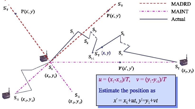
Figure 1: Figure showing the estimated path using interpolation and extrapolation.

As opposed to MADRD, estimation using interpolation depends on localization calls enclosing the point to be estimated rather than last calls. Our intuition is that estimation by interpolation will be more guided by the actual motion than MADRD. If the sensors change the mobility pattern (i.e., speed, direction of path etc.) very frequently MADRD incurs high error in the position estimation. We propose the algorithm MAINT. We proved our intuition by deriving average error for MADRD as well as MAINT. We support the analytical result by simulations. Both the analytical formula as well as simulation studies show that our proposed algorithm incurs significantly lower error than that of MADRD even consuming equal energy.

4 Localization Protocol for Tracking Mobile Sensors

In several applications, a mobile sensor may frequently change its position and direction of its path of mobility with time. A simple strategy for finding its position is the use of standard localization methods at any time. But if the position of the sensor is required frequently, this method is very costly. SFR calls a classical localization operation periodically with a fixed time interval. To respond a query from the base station, a sensor sends its position obtained from the last localization. When a sensor remains still or moves fast, in both cases, the reported position suffers a large error. In DVM, localization is called adaptively with the mobility of the sensors. The time interval for the next call for localization is calculated as the time required to traverse the threshold distance (a distance, traversed by the sensor, location estimation assumed to be error prone) with the velocity of the sensor between last two points in the sequence of localization calls. In case of high mobility, a sensor calls localization frequently. If a sensor suddenly moves with very high speed from rest, error in the estimated location becomes very high. In MADRD, the velocity is calculated from the information obtained from last two localized points. The predictor estimates the position with this velocity and communicates to the query sender. At the localization point, the localized position is reported to the query sender and the distance error is calculated as the distance between the predicted position and reported position. If the error in position estimation exceeds threshold error (application dependent), the predictor appears to be erroneous and localization needs to be triggered more frequently. The calculation of error is necessary every time a localization called. Also, a sensor with high speed calls localizations frequently. We have proposed a method, MAINT, to estimate the current position with better trade off between the energy consumption and accuracy. MAINT uses interpolation which gives better estimation in most cases.

4.1 Mobility Aware Interpolation (MAINT)

In some applications, the base station may need the locations of individual sensors at different times. The location may be required to be attached to the data gathered by the sensors in response to a query. However, the data may not be required immediately. In such cases, the number of localization calls may be reduced by delaying the response. We propose a localization control scheme by estimating positions using interpolation. The sensor holds the queries requiring the the location, into a list, queryPoints and sends the event to the base station padding the time of occurrence. At the following localization point, the sensor sends these two localized positions to each of the query senders in the time interval between these two localization points which are already in the list. The base station estimates the positions with more accuracy by interpolation with this information. The time interval of localization calls is as simple as in SFR. It eliminates all the arithmetic overheads as opposed to MADRD and the error prone nature in sudden change of speeds. Unnecessary calls of localizations for slow sensors may be avoided. To reduce the energy dissipation, the localization method may be called with higher time interval. The localization may be called immediately after receiving the query for real time applications or some special purpose. Each sensor runs a process described by Algorithm 1.

Algorithm 1 (MAINT: Proposed algorithm)

1:Let $(x_{1},y_{1})$ denotes the last localization point occurred at time $t_{1}$.

2:Set $\mathtt{queryPoints}\leftarrow\emptyset$.

3:while (a query received from a sensor $S$ at time $t>t_{1}$) do

4:     Append $S$ to $\mathtt{queryPoints}$, if $S\notin\mathtt{queryPoints}$.

5:     if (response to the query is immediate) or ($t\geq t_{1}+T$) then

6:         Call an optimized localization method

7:         Let $(\hat{x},\hat{y})$ be the location obtained from the method;

8:         while ($\mathtt{queryPoints}\neq\emptyset$) do

9:              Extract a query sender, say $S^{\prime}$, from $\mathtt{queryPoints}$;

10:              Send $t_{1}$, $t$, $(x_{1},y_{1})$ and $(\hat{x},\hat{y})$ to $S^{\prime}$

11:         end while

12:         Set $t_{1}=t$ and $(x_{1},y_{1})$ = $(\hat{x},\hat{y})$.

13:     end if

14:end while

After receiving a message from a sensor, the base station waits until it gets location information of the sender, $S$. If the processing of the message is immediate, the base station may send location query to the node $S$. The base station extracts localization points from the response obtained from $S$ against the location query and estimates the location of $S$ as follows:
 

1:Let $(x_{1},y_{1})$ and $(x_{2},y_{2})$ be the localized positions of $S$ at $t_{1}$ and $t_{2}$ respectively. Let the base station require the position of $S$ at the time $t^{\prime}$.

2:if ($t^{\prime}\in[t_{1},t_{2}]$) then

3:     Calculate the velocity vector as follows:

4:          $\dot{x}=(x_{2}-x_{1})/(t_{2}-t_{1})$;        $\dot{y}=(y_{2}-y_{1})/(t_{2}-t_{1})$;

5:     Estimate the position of $s$ at time $t^{\prime}\in[t_{1},t_{2}$] as follows:

6:          $\hat{x}=x_{1}+\dot{x}(t^{\prime}-t_{1})$;        $\hat{y}=y_{1}+\dot{y}(t^{\prime}-t_{1})$;

7:end if

  
The base station estimates the locations of those sensors only whose events are being processed recently by the base station. The location of a sensor at a particular time instant on demand are estimated from the locations obtained in the previous and next localizations nearest to the time instant.

We explain the proposed algorithm, MAINT, with an example. Figure 2 describes pictorially the algorithm with an example. Suppose, the sensor calls the localization at time $t_{0}$ and gets the position $(x_{1},y_{1})$. Suppose, the sensor receives a query for its location, at time $t_{1}$ from the destination $D_{1}$ (may be a sensor or base station).

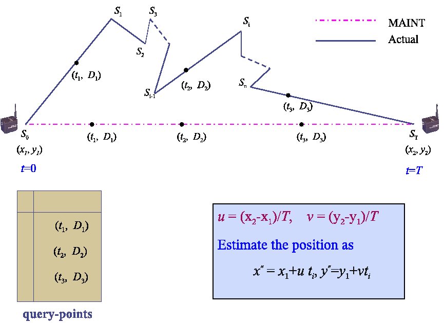
Figure 2: Describing the algorithm with an example.

Instead sending the location immediately, the sensor keeps track of the query inserting $t_{1}$ and $D_{1}$ into a list $\mathtt{queryPoints}$. Similarly, it receives the queries at time $t_{2}$ and $t_{3}$ from the destinations $D_{2}$ and $D_{3}$ respectively. To keep track these query points, $t_{2}$, $D_{2}$ and $t_{3}$, $D_{3}$ are appended in $\mathtt{queryPoints}$. After time $T$ the MAINT calls the localization to know the actual position $(x_{2},y_{2})$. The sensor sends the message consisting of $t_{0}$, $(x_{1},y_{1})$ and $T$, $(x_{2},y_{2})$ corresponding to these two localization points to the query senders $D_{1}$, $D_{2}$ and $D_{3}$. The query senders find the locations of the sensor extracting the information from the message. To reduce the message size, the sensor itself may calculate the velocity from the localization point at $t_{0}$ and that at $T$. Using this velocity, calculate the locations at $t_{1}$, $t_{2}$ and $t_{3}$ and sends the locations to $D_{1}$, $D_{2}$ and $D_{3}$ respectively. It increases arithmetic overhead in the sensor but reduces traffic through the network.

5 Energy and Error Analysis

Localization in static network is very costly. Finding position of mobile sensors, it needs frequent localization calls. We assume, the energy consumption is proportional to the number of localization calls. So we measure energy in terms of number of localization calls. In this work we are reducing the number of localization calls for the shake of energy saving rather than efficient method.

5.1 Mobility Model

The Random Waypoint (RWP) [7, 4] is a commonly used synthetic model for mobility. We carried out the simulation study as well as analysis with RWP mobility model. The parameters used in the model are described as follows:

• Each node moves along a zigzag line from one waypoint to the next. The next waypoint is selected randomly over a given convex area with two parameters time and velocity.

• At the beginning of each leg, a random velocity is drawn from the velocity distribution and reach the next waypoint at random time drawn from the time distribution.

In Figure 3 the sensor starts from $S_{0}(x_{0},y_{0})$ and reaches $S_{T}(x_{T},y_{T})$, the point at time $T$. The sequence of the waypoints attended by the sensor in the time interval $[0,T]$ is $S_{0},S_{1},\cdots,S_{n},S_{T}$.

Figure 3: A snapshot of Actual Path of Sensor under Random Waypoint Model

Let $t_{0}$ and $t_{T}$ be time instances respectively for two consecutive calls of MAINT. The positions of the sensor are known without any error at the time instances $t_{0}$ and $t_{T}$. Estimated positions of the sensor in between $t_{0}$ and $t_{T}$ may be erroneous. Without loss of generality, we assume that $t_{0}=0$, $t_{T}=T$ and $(x_{0},y_{0})=(0,0)$. Because, the error analysis remains similar in between any two consecutive calls of MAINT. We assume, at any waypoint $S_{i}$, the sensor draws the time interval $t_{i+1}$ as well as the velocity vector $(u_{i+1},v_{i+1})$ randomly and independently. The sensor reaches the next waypoint $S_{i+1}$ after the time $t_{i+1}$ with the velocity vector $(u_{i+1},v_{i+1})$. For the sake of simplicity we assume, the time interval follows the exponential distribution with mean $\frac{1}{\lambda}$ and the velocity components $u_{i+1}$ and $v_{i+1}$ are independent and identically distributed with $Normal(0,\sigma)$ at any waypoint for $i=0,1,\cdots,n$. Let $P(x,y)$ be the position of of the sensor at a random time $t$ in $(0,T)$, if the sensor follows the RWP mobility model.

5.2 Actual Motion Analysis: Related Parameters and Expressions

From the theory of probability and stochastic process [9, 2], we can say that the event of occurring waypoints, according to the above mobility model, follows the Poisson Process with parameter $\lambda$. Consider a random variable $N(t)$ that denotes the number of waypoints in the interval $(0,t)$. $N(t)$ follows the Poisson distribution with mean $\lambda t$. The probability mass function (pmf) is

$$\Pr(N(t)=k)=\frac{(\lambda t)^{k}}{k!}e^{-\lambda t},\mbox{~{}~{}~{}~{}for~{}~{}}k=0,1,2,\cdots,\infty.$$ (1)

The sum $T_{i}=t_{1}+t_{2}+\cdots+t_{i}$ (with $T_{0}\equiv 0$) represents the time occurring $i$th waypoint, $S_{i}$. Since $t_{i}$s are independent and identically distributed following exponential distribution with parameter $\lambda$ (mean $\frac{1}{\lambda}$), the random variable $T_{i}$ follows the distribution $\Gamma(\lambda,i)$. The pdf is

$$f_{T_{i}}(\tau)=\frac{\lambda^{i}\tau^{i-1}e^{-\lambda\tau}}{\Gamma(i)}~{}~{}~{}~{}where~{}~{}0<\tau<\infty.$$

Let $(X_{i},Y_{i})$ represent the position of $i$th waypoint, $1\leq i\leq n$. $X_{i}$ and $Y_{i}$ are independent and identically distributed where

$$\begin{array}[]{lclc}X_{i}&=&X_{i-1}+u_{i}t_{i}=u_{1}t_{1}+u_{2}t_{2}+\cdots+u_{i}t_{i}&and\\ Y_{i}&=&Y_{i-1}+v_{i}t_{i}=v_{1}t_{1}+v_{2}t_{2}+\cdots+v_{i}t_{i}\end{array}$$

with $(X_{0},Y_{0})=(0,0)$. The velocity components $u_{i}$ and $v_{i}$ are independent and both follow the distribution $Normal(0,\sigma)$.

Given $n$ waypoints have been occurred by time $\tau$. Let $T_{k}\mid N(\tau)=n$ denote the waiting time of the $k$-th waypoint $(1\leq k\leq n)$ under the given setup.

Basic Result 1

The joint pdf of  $(T_{k-1},t_{k})\mid N(\tau)=n$  for  $2\leq k\leq n$  is

$$f_{T_{k-1}t_{k}}\left((x,y)\mid N(\tau)=n\right)$$

$$= \left\{\begin{array}[]{ll}\frac{n!}{(k-2)!\;(n-k)!}\cdot\frac{x^{k-2}}{\tau^{n}}\left(\tau-x-y\right)^{n-k},&0<x<\tau,~{}0<x+y<\tau\\[5.69054pt] 0,&otherwise.\end{array}\right.$$

Proof: For  $2\leq k\leq n$, $0<x<\tau,0<x+y<\tau$, the probability element

$$\begin{array}[]{rcl}\lx@intercol\@ADDCLASS{ltx_eqn_lefteqn}$\displaystyle\Pr((x<T_{k-1}\leq x+dx,~{}y<t_{k}\leq y+dy)\mid(N(\tau)=n))$\mbox{}\hfil\lx@intercol\\[5.69054pt] &=&\frac{\Pr(x<T_{k-1}\leq x+dx,~{}y<t_{k}\leq y+dy~{}and~{}N(\tau)=n)}{\Pr(N(\tau)=n)}\\[5.69054pt] &=&\Pr(x<T_{k-1}\leq x+dx)\cdot\frac{\Pr(y<t_{k}\leq y+dy\mid T_{k-1}=x)\cdot\Pr((N(\tau)=n)\mid(T_{k}=x+y))}{\Pr(N(\tau)=n)}\\[5.69054pt] &=&\Pr(x<T_{k-1}\leq x+dx)\cdot\Pr(y<t_{k}\leq y+dy)\cdot\frac{\Pr(N(\tau-x-y)=n-k)}{\Pr(N(\tau)=n)}\\[5.69054pt] &=&\frac{\frac{\lambda^{k-1}\,x^{k-2}}{\Gamma(k-1)}\,e^{-\lambda x}\,dx\cdot\lambda\,e^{-\lambda y}\,dy\cdot\frac{\lambda^{n-k}\,(\tau-x-y)^{n-k}}{(n-k)!}\,e^{-\lambda(\tau-x-y)}}{\frac{\lambda^{n}\,\tau^{n}}{n!}\,e^{-\lambda\tau}}\\[8.53581pt] &=&\frac{n!}{(k-2)!\;(n-k)!}\,\cdot\frac{x^{k-2}}{\tau^{n}}~{}(\tau-x-y)^{n-k}\,dx\,dy\end{array}$$

Hence the pdf.

Basic Result 2

The pdf of  $T_{k}\mid N(\tau)=n$  for $1\leq k\leq n$ is given by

$$f_{T_{k}}(x\mid N(\tau)=n)=\left\{\begin{array}[]{lcl}\frac{n!}{(k-1)!\;(n-k)!}\cdot\frac{x^{k-1}}{\tau^{k}}\left(1-\frac{x}{\tau}\right)^{n-k},&&0<x<\tau\\[5.69054pt] 0,&&otherwise.\end{array}\right.$$

Proof: From Result 1, for $2\leq k\leq n$, the pdf of ($T_{k-1}\mid N(\tau)=n$) is

$$\begin{array}[]{rcl}\lx@intercol\@ADDCLASS{ltx_eqn_lefteqn}$\displaystyle f_{T_{k-1}}\left(x\mid N(\tau)=n\right)$\mbox{}\hfil\lx@intercol\\[2.84526pt] &=&\left\{\begin{array}[]{lcl}\frac{n!}{(k-2)!\;(n-k)!}\cdot\frac{x^{k-2}}{\tau^{n}}\cdot\int_{0}^{\tau-x}\left(\tau-x-y\right)^{n-k}\,dy,&&0<x<\tau\\[4.2679pt] 0,&&otherwise.\end{array}\right.\\[11.38109pt] &=&\left\{\begin{array}[]{lcl}\frac{n!}{(k-2)!\;(n-k+1)!}\cdot\frac{x^{k-2}}{\tau^{n}}\cdot\left(\tau-x\right)^{n-k+1},&&0<x<\tau\\[4.2679pt] 0,&&otherwise.\end{array}\right.\end{array}$$

The pdf of  $T_{k}\mid N(\tau)=n$  for  $1\leq k\leq n-1$ is

$$\begin{array}[]{rcl}f_{T_{k}}\left(x\mid N(\tau)=n\right)&=&\left\{\begin{array}[]{lcl}\frac{n!}{(k-1)!\;(n-k)!}\cdot\frac{x^{k-1}}{\tau^{n}}\cdot\left(\tau-x\right)^{n-k},&&0<x<\tau\\[4.2679pt] 0,&&otherwise.\end{array}\right.\end{array}$$

For  $0<x<\tau$, the probability element,

$$\begin{array}[]{rcl}\lx@intercol\@ADDCLASS{ltx_eqn_lefteqn}$\displaystyle\Pr(x<T_{n}\leq x+dx\mid N(\tau)=n)$\mbox{}\hfil\lx@intercol&\\[8.53581pt] &=&\frac{\Pr(x<T_{n}\leq x+dx~{}and~{}N(\tau)=n)}{\Pr(N(\tau)=n)}\\[8.53581pt] &=&\frac{\Pr(x<T_{n}\leq x+dx)\cdot\Pr(N(\tau)=n\mid T_{n}=x)}{\Pr(N(\tau)=n)}\\[8.53581pt] &=&\frac{\Pr(x<T_{n}\leq x+dx)\cdot\Pr(N(\tau-x)=0)}{\Pr(N(\tau)=n)}\\[8.53581pt] &=&\frac{\lambda^{n}\,x^{n-1}}{\Gamma(n)}\,e^{-\lambda x}\,dx\cdot e^{-\lambda(\tau-x)}/\left(\frac{\lambda^{n}\,\tau^{n}}{n!}\,e^{-\lambda\tau}\right)\\[8.53581pt] &=&n\cdot\frac{x^{n-1}}{\tau^{n}}\,dx\end{array}$$

Hence, the pdf of  $T_{k}\mid N(\tau)=n$  is followed, for $1\leq k\leq n$.

Basic Result 3

$E(T_{k}\mid N(\tau)=n)=\frac{k\,\tau}{n+1}$ and $E(T_{k}^{2}\mid N(\tau)=n)=\frac{k(k+1)\,\tau^{2}}{(n+1)(n+2)}$, for  $1\leq k\leq n$.

Proof: Using the pdf as in Result 2,  for  $1\leq k\leq n$, we may write the expected values $E(T_{k}^{m}\mid N(\tau)=n)$ as follows:

$$\begin{array}[]{rcl}{E(T_{k}^{m}\mid N(\tau)=n)}&=&\int_{0}^{\tau}x^{m}\,f_{T_{k}}\left(x\mid N(\tau)=n\right)\,dx\\[5.69054pt] &=&\frac{n!\;\tau^{m}}{(k-1)!\,(n-k)!}\int_{0}^{\tau}\left(\frac{x}{\tau}\right)^{m+k-1}\,\left(1-\frac{x}{\tau}\right)^{n-k}\,\frac{dx}{\tau}\\[8.53581pt] &=&\frac{n!\;\tau^{m}}{(k-1)!\,(n-k)!}\int_{0}^{1}x^{m+k-1}\,\left(1-x\right)^{n-k}\,dx\\[8.53581pt] &=&\frac{n!\;\tau^{m}}{(k-1)!\,(n-k)!}\cdot\frac{\Gamma(m+k)\;\Gamma(n-k+1)}{\Gamma(n+m+1)}\\[8.53581pt] &=&\frac{n!\;(m+k-1)!}{(k-1)!\;(n+m)!}~{}\tau^{m}\end{array}$$

Substituting, $m$ by $1$ and $2$,  we may have the expectations   $E(T_{k}\mid N(\tau)=n)$   and   $E(T_{k}^{2}\mid N(\tau)=n)$,   for  $1\leq k\leq n$. Hence the result follows.

Let $t_{k}\mid N(\tau)=n$ represent the time interval between the $(k-1)$th and the $k$th waypoints under the given setup when we are given that exactly $n$ waypoints have occurred in the interval $(0,\tau)$.

Basic Result 4

The density function of  $t_{k}\mid N(\tau)=n$,  for  $1\leq k\leq n$  is

$$f_{t_{k}}(y\mid N(\tau)=n)=\left\{\begin{array}[]{ll}\frac{n}{\tau}\left(1-\frac{y}{\tau}\right)^{n-1},&0\leq y<\tau\\[5.69054pt] 0,&otherwise.\end{array}\right.$$

Proof: The random variable $T_{1}=t_{1}$. The distribution of  ($t_{1}\mid N(\tau)=n$) is same as the distribution of ($T_{1}\mid N(\tau)=n$). From the Result 1, the distribution of   $t_{k}\mid N(\tau)=n$  for $2\leq k\leq n$ is

$$\begin{array}[]{rcl}\lx@intercol\@ADDCLASS{ltx_eqn_lefteqn}$\displaystyle f_{t_{k}}\left(y\mid N(\tau)=n\right)$\mbox{}\hfil\lx@intercol\\[2.84526pt] &=&\left\{\begin{array}[]{ll}\frac{n!}{(k-2)!(n-k)!}\cdot\frac{(\tau-y)^{n-1}}{\tau^{n}}\int_{0}^{\tau-y}(\frac{x}{\tau-y})^{k-2}(1-\frac{x}{\tau-y})^{n-k}\,\frac{dx}{\tau-y},&0\leq y<\tau\\[5.69054pt] 0,&otherwise.\end{array}\right.\\[11.38109pt] &=&\left\{\begin{array}[]{lcl}\frac{n!}{(k-2)!(n-k)!}\cdot\frac{(\tau-y)^{n-1}}{\tau^{n}}\int_{0}^{1}t^{k-2}\,(1-t)^{n-k}\,dt,&&0\leq y<\tau\\[5.69054pt] 0,&&otherwise.\end{array}\right.\\[11.38109pt] &=&\left\{\begin{array}[]{lcl}\frac{n!}{(k-2)!(n-k)!}\cdot\frac{(\tau-y)^{n-1}}{\tau^{n}}\cdot\frac{\Gamma(k-1)\,\Gamma(n-k+1)}{\Gamma(n)},&&0\leq y<\tau\\[5.69054pt] 0,&&otherwise.\end{array}\right.\end{array}$$

Thus the pdf of  $t_{k}\mid N(\tau)=n$  for $1\leq k\leq n$ is

$$\begin{array}[]{rcl}f_{t_{k}}\left(y\mid N(\tau)=n\right)&=&\left\{\begin{array}[]{lcl}\frac{n}{\tau}\,\left(1-\frac{y}{\tau}\right)^{n-1},&&0\leq y<\tau\\[8.53581pt] 0,&&otherwise.\end{array}\right.\\[-8.53581pt] \end{array}$$

Basic Result 5

$E(t_{k}\mid N(\tau)=n)$ = $\frac{\tau}{n+1}$ and $E(t_{k}^{2}\mid N(\tau)=n)$ = $\frac{2\tau^{2}}{(n+1)(n+2)}$

Proof: Using the pdf as in Result 2,   for   $1\leq k\leq n$,   we have

$$\begin{array}[]{rcl}E(t_{k}^{m}\mid N(\tau)=n)&=&\int_{0}^{\tau}y^{m}\,f_{t_{k}}\left(y\mid N(\tau)=n\right)\,dy\\[8.53581pt] &=&n\,\tau^{m}\int_{0}^{\tau}\left(\frac{y}{\tau}\right)^{m}\,\left(1-\frac{y}{\tau}\right)^{n-1}\,\frac{dy}{\tau}\\[8.53581pt] &=&n\,\tau^{m}\int_{0}^{1}y^{m}\,\left(1-y\right)^{n-1}\,dy\\[8.53581pt] &=&n\,\tau^{m}\cdot\frac{\Gamma(m+1)\;\Gamma(n)}{\Gamma(n+m+1)}\\[8.53581pt] &=&\frac{n!\;m!}{(n+m)!}~{}\tau^{m}\end{array}$$

Putting $m=1$ and $m=2$ in the above relation, we can have $E(t_{k}\mid N(\tau)=n)$ and $E(t_{k}^{2}\mid N(\tau)=n)$, for $1\leq k\leq n$.

Basic Result 6

$E(X_{k}\mid N(\tau)=n)=0$ and $E(X_{k}^{2}\mid N(\tau)=n)$ = $\frac{2k\,\sigma^{2}\,\tau^{2}}{(n+1)\,(n+2)}$,  for  $1\leq k\leq n$.

Proof: $X_{k}=\sum_{i=1}^{k}u_{i}\,t_{i}$, for $1\leq k\leq n$  and $t_{k}$ s and $u_{k}$ s are independent.

$$\begin{array}[]{rcl}E(X_{k}\mid N(\tau)=n)&=&E\left(\left(\sum_{i=1}^{k}u_{i}\,t_{i}\right)\mid N(\tau)=n\right)\\[5.69054pt] &=&\sum_{i=1}^{k}E\left(u_{i}\right)\,E\left(t_{i}\mid N(\tau)=n\right),\\ &&\hskip 14.22636pt\mbox{since, $u_{i}$\,s are independent on $t_{i}$\,s and $N(\tau)=n$}\\ &=&0,\hskip 73.97733pt\mbox{since $E(u_{i})=0$.}\end{array}$$

Similarly,   $E(X_{k}^{2}\mid N(\tau)=n)$

$$\begin{array}[]{rl}&=E\left(\left(\sum_{i=1}^{k}u_{i}\,t_{i}\right)^{2}\mid N(\tau)=n\right)\\[8.53581pt] &=E\left(\left(\sum_{i=1}^{k}u_{i}^{2}\,t_{i}^{2}+2\,\sum_{i<j=1}^{k}u_{i}\,u_{j}\,t_{i}\,t_{j}\right)\mid N(\tau)=n\right)\\[2.84526pt] &=\sum\limits_{i=1}^{k}E(u_{i}^{2})\,E(t_{i}^{2}\mid N(\tau)=n)+2\sum\limits_{i<j=1}^{k}E(u_{i})\,E(u_{j})\,E(t_{i}\,t_{j}\mid N(\tau)=n)\\[0.28453pt] &=\sigma^{2}\sum\limits_{i=1}^{k}E(t_{i}^{2}\mid N(\tau)=n),~{}~{}~{}~{}~{}~{}~{}~{}~{}~{}\mbox{since, $E(u_{i})=0$ and $E(u_{i}^{2})=\sigma^{2}$}\\[8.53581pt] &=\frac{2k\,\sigma^{2}\,\tau^{2}}{(n+1)\,(n+2)},~{}~{}~{}~{}~{}~{}~{}~{}~{}~{}~{}~{}~{}~{}~{}~{}~{}~{}~{}~{}~{}\mbox{using Result~{}\ref{res:Exp:t_k|n}.}\\[-8.53581pt] \end{array}$$

5.2.1 Actual Position of Sensor

We analyze the motion of the sensor in between two consecutive calls of localization. Because, the pattern of the motion remains similar in between any two consecutive localization points. Let $P(x,y)$ be the position of the sensor at a random time $t$, $0<t<T$. Consider the random variable $(X,Y)$ that represents the position of $P$. Let $i$ waypoints occur in the interval $(0,t)$, i.e. $0\leq T_{i}\leq t<T_{i+1}$. Given $N(t)=i$. Then we have

$X=X_{i}+(t-T_{i})u_{i+1}$          $Y=Y_{i}+(t-T_{i})v_{i+1}$

for   $i=0,1,2,\ldots,\infty$ where $T_{0}=0$ and $(X_{0},Y_{0})=(0,0)$.

Theorem 1

$E(X\mid N(t)=i)=0$ and $E(X^{2}\mid N(t)=i)$ = $\frac{2}{i+2}\,\sigma^{2}\,t^{2}$.

Proof: Consider  $X=X_{i}+(t-T_{i})\,u_{i+1}$, given  $N(t)=i$, for a fixed  $t\in(0,T)$.

$$\begin{array}[]{rcl}E(X\mid N(t)=i)&=&E(X_{i}\mid N(t)=i)+E((t-T_{i})\mid N(t)=i)\,E(u_{i+1})\\ &=&0,~{}~{}~{}~{}~{}~{}~{}~{}~{}~{}~{}~{}~{}~{}\mbox{using ~{}$E(u_{i+1})=0$~{} and ~{}Result~{}\ref{res:Exp:X_k|n}.}\end{array}$$

Similarly,  $E(X^{2}\mid N(t)=i)$

$$\begin{array}[]{rcl}&=&E(X_{i}^{2}\mid N(t)=i)+E(u_{i+1}^{2})\,E((t-T_{i})^{2}\mid N(t)=i)\\[0.28453pt] &&\hskip 142.26378pt+2\,E(u_{i+1})\,E((t-T_{i})\mid N(t)=i)\\ &=&E(X_{i}^{2}\mid N(t)=i)+\sigma^{2}\,(t^{2}-2t\;E(T_{i}\mid N(t)=i)+E(T_{i}^{2}\mid N(t)=i))\\[1.42262pt] &=&\frac{2i\,\sigma^{2}\,t^{2}}{(i+1)\,(i+2)}+\sigma^{2}\,\left(t^{2}-2t\;\frac{i\,t}{i+1}+\frac{i\,(i+1)\,t^{2}}{(i+1)\,(i+2)}\right),~{}~{}~{}~{}\mbox{using Result~{}\ref{res:Exp:T_k|n} and \ref{res:Exp:X_k|n}.}\\ &=&\frac{2}{i+2}\;\sigma^{2}\,t^{2}.\\[-8.53581pt] \end{array}$$

Theorem 2

The expectation of $X$ and $X^{2}$ are given by $E(X)=0$ and

$$E(X^{2})=2\sigma^{2}\left(\frac{t}{\lambda}-\frac{1}{\lambda^{2}}+\frac{1}{\lambda^{2}}e^{-\lambda t}\right).$$

Proof: The random variable $X$ represents the $x$-coordinate of the sensor at time $t$. In the a particular time instant the expected value of $X^{2}$ is given by

$$\begin{array}[]{rcl}E(X^{2})&=&E[E(X^{2}\mid N(t)=i)]\\[5.69054pt] &=&E\left(\frac{2\sigma^{2}t^{2}}{i+2}\right),~{}~{}\mbox{using Theorem~{}\ref{cor:Exp:X|i}}\\[8.53581pt] &=&2\sigma^{2}t^{2}\sum\limits_{i=0}^{\infty}\frac{1}{i+2}\Pr(N(t)=i)\\[11.38109pt] &=&2\sigma^{2}t^{2}\sum\limits_{i=0}^{\infty}\frac{1}{i+2}\,\frac{(\lambda t)^{i}}{i\,!}e^{-\lambda t}\\[14.22636pt] &=&2\sigma^{2}t^{2}\left(\frac{1}{\lambda t}-\frac{1}{\lambda^{2}t^{2}}+\frac{1}{\lambda^{2}t^{2}}e^{-\lambda t}\right)\\[11.38109pt] &=&2\sigma^{2}\left(\frac{t}{\lambda}-\frac{1}{\lambda^{2}}+\frac{1}{\lambda^{2}}e^{-\lambda t}\right)\\[-5.69054pt] \end{array}$$

5.3 Estimation by MAINT and Error Analysis

Assume two consecutive calls of MAINT occur at the times $0$ and $T$. In Figure 4, $S_{0},S_{1},\ldots,S_{n},S_{T}$ is the actual path of the sensor in between the times $0$ and $T$.

Figure 4: Showing position estimates at an intermediate point by MADRD and MAINT.

Let $P(x,y)$ be the actual position of the sensor at a random time $t\in(0,T)$ when it follows the said RWP mobility model. Let $P^{\prime}\,(x_{est},y_{est})$ be the estimated position of the sensor at $t$ according to MAINT. Let $(X_{est},Y_{est})$ denotes the random variable to estimated position $P^{\prime}$ by MAINT at time $t$. Then we have

$$X_{est}=\frac{X_{T}}{T}t,~{}~{}~{}~{}Y_{est}=\frac{Y_{T}}{T}t$$

where $(X_{T},Y_{T})$ is the random position of the sensor at time $T$.

5.3.1 Error Analysis

In the analysis, we consider RWP mobility model. We assume the waypoints follows the Poisson process. Since localizations occur at time $0$ and $T$, we consider the motion in the time interval $[0,T]$. For error calculation we take a location estimation at a random time $t\in[0,T]$. Due to the memory less property of Poison process, we may break the complete scenario in two independent Poisson processes with same parameter, one in the interval $[0,t]$ and another in $[t,T]$. As a whole, these two processes represent the same process as in $[0,T]$. Suppose, $N^{\prime}(\tau)=m$ denote the event that $m$ waypoints occur in $[t,T]$.

Theorem 3

$\Pr(N^{\prime}(\tau)=m)=\Pr(N(\tau-t)=m)$.

Proof: It follows from the memory less property of Poisson process [2].

Theorem 4

$\Pr(N(t)=i,N^{\prime}(T)=j)=\frac{\lambda^{i+j}e^{-\lambda T}}{i!\,j!}t^{i}(T-t)^{j}$.

Proof: From the Poisson process we can say that the events $N(t)=i$ and $N^{\prime}(T)=j$ are independent. Therefore,

$$\Pr(N(t)=i,N^{\prime}(T)=j)=\Pr(N(t)=i)\Pr(N^{\prime}(T)=j).$$

From the equation (1) and the Theorem 3 we have

$$\Pr(N(t)=i,N^{\prime}(T)=j) = \Pr(N(t)=i)\Pr(N(T-t)=j)$$

$$= \frac{(\lambda t)^{i}}{i!}\,e^{-\lambda t}\cdot\frac{(\lambda(T-t))^{j}}{j!}\,e^{-\lambda(T-t)}$$

$$= \frac{\lambda^{i+j}\,e^{-\lambda T}}{i!\,j!}t^{i}(T-t)^{j}$$

Expected Error in MAINT

Consider a random time $t$ in the interval $(0,T)$. Let $S_{1}$, $S_{2}$, $\cdots$, $S_{i}$ be $i$ waypoints occurred in $[0,t]$ and $j$ waypoints $S_{i+1}$, $S_{i+2}$, $\cdots$, $S_{i+j}$ occur in the time interval $[t,T]$. Under this setup, the actual position of the sensor at time $t$ is given by the random variable $(X,Y)$ where

$$X=X_{i}+(t-T_{i})u_{i+1}$$

$$Y=Y_{i}+(t-T_{i})v_{i+1}.$$

Since, the process in $[0,t]$ and in $[t,T]$ are independent to each other, we may assume the waypoints $S_{i+1}$, $S_{i+2}$, $\cdots$, $S_{i+j}$ occurs just like the system starts from the time $t$ where the position of the sensor is $(X,Y)$. Due to the memory less property of the Poisson Process, we may obtain the time occurrences of the waypoints $S_{i+1}$, $S_{i+2}$, $\cdots$, $S_{i+j}$ form the same Poisson process over the time interval $[0,T-t]$ with an additional time $t$. Let $T^{\prime}_{k}$ and $t^{\prime}_{k}$ denote the time of occurrence of the position of the waypoint $S_{i+k}$ and time interval between two waypoints of the motion of the sensor in $[0,T-t]$. If $(X^{\prime}_{k},Y^{\prime}_{k})$ denote the the random position of the waypoint $S_{i+k}$ taking $(X,Y)$ as the origin, we have

$$X^{\prime}_{k}=X^{\prime}_{k-1}+t^{\prime}_{k}u_{i+k}=\sum_{m=1}^{k}t^{\prime}_{m}u_{i+m},$$

$$Y^{\prime}_{k}=Y^{\prime}_{k-1}+t^{\prime}_{k}v_{i+k}=\sum_{m=1}^{k}t^{\prime}_{m}v_{i+m}$$

for $k=0,1,2,\ldots,\infty$ where $T^{\prime}_{0}=0$ and $(X^{\prime}_{0},y^{\prime}_{0})=(0,0)$.

The random velocity vector at any waypoint is independent to time of occurrence of the waypoint. So $(X_{i},Y_{i})$ and $(X^{\prime}_{k},Y^{\prime}_{k})$ are independent for $i\geq 1,k\geq 1$. If we assume the coordinates of the waypoint $S_{i+j}$ in the whole process over $[0,T]$ as $(X_{i+j},Y_{i+j})$, we have $X_{i+j}=X+X^{\prime}_{j}$, $Y_{i+j}=Y+Y^{\prime}_{j}$ and $T_{i+j}=t+T^{\prime}_{j}$. If $(X^{\prime},Y^{\prime})$ denote the position of the sensor at time $T$ due to the process over $[0,T-t]$ under the condition that $N^{\prime}(T)=j$, i.e., $N(T-t)=j$ then

$X^{\prime}=X^{\prime}_{j}+(T-t-T^{\prime}_{j})u_{i+j+1},~{}~{}~{}~{}~{}~{}~{}~{}Y^{\prime}=Y^{\prime}_{j}+(T-t-T^{\prime}_{j})v_{i+j+1}.$

The position of the sensor at time $T$, $(X_{T},Y_{T})$, due to the process over $[0,T]$ under the conditions that $N(t)=i$ and $N^{\prime}(T)=j$, may be obtained as

$X_{T}=X+X^{\prime}_{j}+(T-t-T^{\prime}_{j})u_{i+j+1}=X+X^{\prime},$

$Y_{T}=Y+Y^{\prime}_{j}+(T-t-T^{\prime}_{j})v_{i+j+1}=Y+Y^{\prime}.$

Therefore, the estimated positions at time $t$ may written as:

$X_{est}=\frac{X+X^{\prime}}{T}\,t,~{}~{}~{}~{}~{}~{}~{}~{}~{}~{}Y_{est}=\frac{Y+Y^{\prime}}{T}\,t$

Let $error_{t}$ denote the expected squared error in the position estimation by MAINT at a random time $t$ in $[0,T]$. Thus, $error_{t}$ can be expressed as:

$$\begin{array}[]{rcl}error_{t}&=&E\left[(X-X_{est})^{2}+(Y-Y_{est})^{2}\right]\\[2.84526pt] &=&2E\left[\left(X-X_{est}\right)^{2}\right],~{}~{}\mbox{since $X-X_{est}$ and $Y-Y_{est}$ are iid}\\[5.69054pt] &=&2E\left[\left(X-\frac{X+X^{\prime}}{T}\,t\right)^{2}\right]\\[8.53581pt] &=&2E\left[\left\{\left(1-\frac{t}{T}\right)X-\frac{t}{T}X^{\prime}\right\}^{2}\right]\\[5.69054pt] &=&2\left[\left(1-\frac{t}{T}\right)^{2}E(X^{2})+\frac{t^{2}}{T^{2}}E\left(X^{\prime 2}\right)-2\frac{t}{T}\left(1-\frac{t}{T}\right)E(XX^{\prime})\right]\end{array}$$ (3)

Theorem 5

The expectation of $X^{\prime}$ and $X^{\prime 2}$ are given by $E(X^{\prime})=0$ and

$E(X^{\prime 2})=2\sigma^{2}\left\{\frac{T-t}{\lambda}-\frac{1}{\lambda^{2}}+\frac{1}{\lambda^{2}}\,e^{-\lambda(T-t)}\right\}.$

Proof: We have seen that $X^{\prime}=X^{\prime}_{j}+(T-t-T^{\prime}_{j})u_{i+j+1}$ is the $x$-coordinate of the sensor at time $T-t$ in the process over $[0,T-t]$. So $X^{\prime}$ has similar properties as $X$ except $N^{\prime}(T)=j$, i.e. $N(T-t)=j$ instead of $N(t)=i$. The event $N^{\prime}(T)$ is independent with the scenario prior to the time $t$, i.e. independent with $N(T)$. Thus, the result follows from Theorem 2 replacing $T-t$ instead of $t$.

Theorem 6

Given $N(t)=i$ and $N^{\prime}(T)=j$ for a particular time $t\in[0,T]$. The expectation of $XX^{\prime}$ may be given as

$E\left[XX^{\prime}\mid N(t)=i,N^{\prime}(T)=j\right]=\frac{\sigma^{2}t(T-t)}{(i+1)(j+1)},~{}~{}~{}~{}~{}~{}~{}~{}for~{}~{}i,j\geq 0.$

Proof: Under the given condition $N(t)=i$ and $N^{\prime}(T)=j$ for a particular time $t\in[0,T]$, we know $X=X_{i}+(t-T_{i})u_{i+1}$ and $X^{\prime}=X^{\prime}_{j}+(T-t-T^{\prime}_{j})u_{i+j+1}$ as stated earlier. Therefore, we have

$$\begin{array}[]{rcl}\lx@intercol\@ADDCLASS{ltx_eqn_lefteqn}$\displaystyle E\left[XX^{\prime}\mid N(t)=i,N^{\prime}(T)=j\right]$\mbox{}\hfil\lx@intercol\\[2.84526pt] &=&E\left[\left\{X_{i}+(t-T_{i})u_{i+1}\right\}\left\{X^{\prime}_{j}+(T-t-T^{\prime}_{j})u_{i+j+1}\right\}\right]\\[2.84526pt] &=&E(t-T_{i})\left\{E\left(u_{i+1}X^{\prime}_{j}\right)+E\left(T-t-T^{\prime}_{j}\right)E\left(u_{i+1}u_{i+j+1}\right)\right\}\\[2.84526pt] &=&\left\{\begin{array}[]{lrl}E(t-T_{i})E\left(u_{i+1}X^{\prime}_{j}\right),&~{}~{}~{}~{}~{}~{}for&i\geq 0,~{}j\geq 1\\[2.84526pt] (T-t)E(t-T_{i})E\left(u_{i+1}^{2}\right),&for&i\geq 0,~{}j=0\end{array}\right.\\[11.38109pt] &=&\left\{\begin{array}[]{lrl}E(t-T_{i})E\left(t^{\prime}_{1}\right)E\left(u_{i+1}^{2}\right),&~{}~{}~{}~{}~{}~{}for&i\geq 0,~{}j\geq 1\\[2.84526pt] (T-t)E(t-T_{i})E\left(u_{i+1}^{2}\right),&for&i\geq 0,~{}j=0\end{array}\right.\\[11.38109pt] &=&\left\{\begin{array}[]{lrl}\sigma^{2}\frac{T-t}{j+1}(t-\frac{it}{i+1}),&~{}~{}~{}~{}~{}~{}for&i\geq 0,~{}j\geq 1\\[2.84526pt] \sigma^{2}(T-t)(t-\frac{it}{i+1}),&for&i\geq 0,~{}j=0\end{array}\right.\\[14.22636pt] &=&\frac{\sigma^{2}\,t(T-t)}{(i+1)(j+1)},~{}~{}~{}~{}~{}~{}for~{}~{}i\geq 0,~{}j\geq 0\\[-14.22636pt] \end{array}$$

Theorem 7

For a particular $t\in[0,T]$, the expectation of $XX^{\prime}$ is given as

$E(XX^{\prime})=\frac{\sigma^{2}}{\lambda^{2}}\left\{1-e^{-\lambda t}-e^{-\lambda(T-t)}+e^{-\lambda T}\right\}.$

Proof: The random variables $X$ and $X^{\prime}$ represent the positions of the sensor in the decomposed motions of the sensor into intervals $[0,t]$ and $[t,T]$ as discussed earlier. The expectation of $XX^{\prime}$ is given as

$$\begin{array}[]{rcl}E(XX^{\prime})&=&E\left[E\left[XX^{\prime}\mid N(t)=i,N^{\prime}(T)=j\right]\right]\\[5.69054pt] &=&E\left[\frac{\sigma^{2}t(T-t)}{(i+1)(j+1)}\right],~{}~{}~{}~{}\mbox{using Theorem~{}\ref{theo:Exp:XX'|ij}}\\[5.69054pt] &=&\sum\limits_{i=0}^{\infty}\sum\limits_{j=0}^{\infty}\left[\frac{\sigma^{2}t(T-t)}{(i+1)(j+1)}\,\cdot\Pr(N(t)=i,N^{\prime}(T)=j)\right]\\[8.53581pt] &=&\sum\limits_{i=0}^{\infty}\sum\limits_{j=0}^{\infty}\left[\frac{\sigma^{2}t(T-t)}{(i+1)(j+1)}\cdot\frac{\lambda^{i+j}\;t^{i}(T-t)^{j}}{i!\;j!}\,e^{-\lambda T}\right],\mbox{by Theorem\,\ref{theo:NN'}}\\[8.53581pt] &=&\frac{\sigma^{2}}{\lambda^{2}}\,e^{-\lambda T}\sum\limits_{i=0}^{\infty}\frac{\lambda^{i+1}t^{i+1}}{(i+1)!}\sum\limits_{j=0}^{\infty}\frac{\lambda^{j+1}(T-t)^{j+1}}{(j+1)!}\\[5.69054pt] &=&\frac{\sigma^{2}}{\lambda^{2}}\,e^{-\lambda T}\sum\limits_{i=1}^{\infty}\frac{\lambda^{i}t^{i}}{i!}\sum\limits_{j=1}^{\infty}\frac{\lambda^{j}(T-t)^{j}}{j!}\\[8.53581pt] &=&\frac{\sigma^{2}}{\lambda^{2}}\,e^{-\lambda T}\left(e^{\lambda t}-1\right)\left(e^{\lambda(T-t)}-1\right)\\[8.53581pt] &=&\frac{\sigma^{2}}{\lambda^{2}}\left\{1-e^{-\lambda t}-e^{-\lambda(T-t)}+e^{-\lambda T}\right\}\\[-11.38109pt] \end{array}$$

Using the Theorems 2,5,7, the equation (3) reduces to the following:

$$\begin{array}[]{rcl}error_{t}&=&2\left[\left(1-\frac{t}{T}\right)^{2}E(X^{2})+\frac{t^{2}}{T^{2}}E\left(X^{\prime 2}\right)-2\frac{t}{T}\left(1-\frac{t}{T}\right)E(XX^{\prime})\right]\\[8.53581pt] &=&\frac{4\sigma^{2}}{\lambda^{2}T^{2}}\left[t^{2}\left\{\lambda(T-t)-1+e^{-\lambda(T-t)}\right\}+(T-t)^{2}\left(\lambda t-1+e^{-\lambda t}\right)\right.\\[5.69054pt] &&\left.-\left(1+e^{-\lambda T}\right)t(T-t)+t(T-t)\,e^{-\lambda t}+t(T-t)\,e^{-\lambda(T-t)}\right]\end{array}$$

Therefore, the average of squared error, denoted by $error(avg)$, in the location estimation by MAINT is given as follows:

$$\begin{array}[]{rcl}error(avg)&=&\frac{1}{T}\int\limits_{0}^{T}error_{t}~{}dt\\[5.69054pt] &=&\frac{4\sigma^{2}}{\lambda^{2}T^{3}}\left[\int_{0}^{T}t^{2}\left\{\lambda(T-t)-1+e^{-\lambda(T-t)}\right\}\,dt\right.\\[5.69054pt] &&+\int_{0}^{T}(T-t)^{2}\left(\lambda t-1+e^{-\lambda t}\right)\,dt-\left(1+e^{-\lambda T}\right)\int_{0}^{T}t(T-t)\,dt\\[5.69054pt] &&+\left.\int_{0}^{T}t(T-t)\,e^{-\lambda t}\,dt+\int_{0}^{T}t(T-t)\,e^{-\lambda(T-t)}\,dt\right]\\[5.69054pt] &=&\frac{4\sigma^{2}}{\lambda^{2}T^{3}}\left[2\int_{0}^{T}t^{2}\left\{\lambda(T-t)-1+e^{-\lambda(T-t)}\right\}\,dt\right.\\[5.69054pt] &&-\left(1+e^{-\lambda T}\right)\frac{T^{3}}{6}+\left.2\int_{0}^{T}t(T-t)\,e^{-\lambda(T-t)}\,dt\right],\\ &&\hskip 56.9055pt\mbox{by fundamental theory of integral calculus}\\[5.69054pt] &=&\frac{4\sigma^{2}}{\lambda^{2}T^{3}}\left[2\int_{0}^{T}\left(\lambda T\,t^{2}-\lambda t^{3}-t^{2}\right)\,dt-\left(1+e^{-\lambda T}\right)\frac{T^{3}}{6}\right.\\[2.84526pt] &&+\left.2T\,e^{-\lambda T}\int_{0}^{T}t\,e^{\lambda t}\,dt\right]\\[5.69054pt] &=&\frac{4\sigma^{2}}{\lambda^{2}T^{3}}\left[2\left(\frac{\lambda T^{4}}{12}-\frac{T^{3}}{3}\right)-\left(1+e^{-\lambda T}\right)\frac{T^{3}}{6}\right.\\[5.69054pt] &&+\left.2T\,e^{-\lambda T}\left(\frac{1}{\lambda^{2}}-\frac{1}{\lambda^{2}}e^{\lambda T}+\frac{T}{\lambda}e^{\lambda T}\right)\right]\\[5.69054pt] &=&\frac{4\sigma^{2}}{\lambda^{2}T^{3}}\left(\frac{\lambda T^{4}}{6}-\frac{5T^{3}}{6}+\frac{2T^{2}}{\lambda}-\frac{2T}{\lambda^{2}}+\frac{2T}{\lambda^{2}}\,e^{-\lambda T}-\frac{T^{3}}{6}\,e^{-\lambda T}\right)\\[5.69054pt] &=&\frac{2\sigma^{2}}{3\lambda^{2}}\left[\lambda T-5+\frac{12}{\lambda T}-\frac{12}{\lambda^{2}T^{2}}+\frac{12}{\lambda^{2}T^{2}}\,e^{-\lambda T}-e^{-\lambda T}\right]\end{array}$$

If we assume $T$ and $\lambda$ grow with $\frac{T}{\lambda}=constant=C$, we get

$$\begin{array}[]{rcl}\lx@intercol\@ADDCLASS{ltx_eqn_lefteqn}$\displaystyle error(avg)$\mbox{}\hfil\lx@intercol\\[5.69054pt] &=&\frac{2\sigma^{2}}{3}\left[C-\frac{5\,C^{2}}{T^{2}}+\frac{12\,C^{3}}{T^{4}}-\frac{12\,C^{4}}{T^{6}}+\frac{12\,C^{4}}{T^{6}}\,e^{-T^{2}/C}-e^{-T^{2}/C}\right]\\[8.53581pt] &=&\frac{2\sigma^{2}\,C}{3},~{}~{}~{}~{}~{}as~{}~{}~{}T\rightarrow\infty~{}~{}with~{}~{}T=C\,\lambda\end{array}$$

From the above result, we see that the average error approaches to zero when $T$, the time period of localizations, tends to zero. The error grows as $T$ becomes large. It is very important to see that as $\lambda$ becomes very large, i.e., sensor changes its direction more frequently, the error becomes very small. If both $T$ and $\lambda$ grows with constant ratio i.e., $\frac{T}{\lambda}=constant$, the error approaches to a constant value. Therefore, if we have prior knowledge of the rate of direction of the motion sensors, we well control the energy with an acceptable level of error by adjusting the value of $C$.

6 Analysis by Simulations

Simulation studies were carried out using ns-2 [1] to compare the performance of the proposed technique with that of MADRD. In the simulation study, we concentrated mainly on the average error distance for different number of localization counts. We assume that the sensors move with RWP mobility model with parameters as in Table 1.

Mobility model	Random Waypoint Model
Velocity components distribution	$Normal(0,\sigma)$, $\sigma=5.0$ unit
Time gap between waypoints distribution	Exponential mean $\frac{1}{\lambda}=10.0$ sec

Table 1: Relevant parameters used in simulation

In this work, velocity components are chosen from independent Normal distribution and time interval between any pair of consecutive waypoints is chosen from the Exponential distribution. During the simulation, we use the parameters described in Table 1. In this model, the time is measured in $sec$. The velocities are measured in $unit/sec$. The error in position are measured in distance unit (i.e., $unit$ as in Table 1).

The simulation process was carried out over for a time span of $100\,secs$. Using MADRD and MAINT, we estimate the position of a mobile sensor at a random time in $[0,100\,secs]$. The error for these estimated positions are computed with the actual positions. We also observed the number of localization calls in $[0,100\,secs]$. The experiment is approximately repeated $10000$ times. The data are grouped with respect to number of localization calls. In Figure 5, we plot the average error for different number of localization counts.

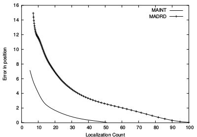
Figure 5: Average error and localization counts for MADRD and the proposed technique.

This figure shows that MAINT performs uniformly better than MADRD. For fixed error level, the localization count and hence the energy consumption in MAINT is significantly lower. Also, for comparable numbers of localization count, MAINT has much lower average error. It estimates the position of a sensor with less error and even consuming less energy. MAINT locates a mobile sensor with nearly exact position of the sensor consuming approximately half energy than that of MADRD. MAINT requires higher memory to hold the history of location queries. We can hold limited number of most recent query points. However, MAINT saves the valuable energy at the cost of cheap memory.

In Figure 6, we compare expected error in position estimation using MAINT with an expression.

Figure 6: Average error in estimation by the proposed technique and theoretical analysis.

This simulation was carried out under the same RWP model in C++ environment. In the course of this simulation, MAINT calls localization procedure with fixed time period $T$. This process is repeated at least $100$ times for a particular value of $T$. The average error are plotted with respect to several values of $T$ in Figure 6. This shows that error may be computed from the deduced expression. Simulation studies with $\frac{T}{\lambda}=50.0$ and $\sigma=10.0$ are shown in the Figure 7.

Figure 7: Average error in estimation by the proposed technique with $\frac{T}{\lambda}=50.0$.

It shows the asymptotic nature of the average error. This plotting shows that the average error becomes stable, if $T$ varies with $\frac{T}{\lambda}=constant$. However, from Figure 6 and 7, we observe that our theoretical analysis well supported by the simulation studies.

7 Conclusion

The technique, proposed in this paper, estimates the location of a mobile sensor. Tilak et al. [16] proposed MADRD, which uses extrapolation and the position of the sensor is estimated by the velocity in between last two localization points. In our proposed method MAINT, we use interpolation. The velocity is calculated from the last and next localization points. In the simulation studies, we see that MAINT estimates the position of the sensor with much lower error than that of MADRD. If the parameters of the model are known, at any moment, the error in the position estimation may be computed from the deduced expression, instead using actual position.

The time interval can control the energy dissipation. A constant error limit can be maintained if the time period of localization increases proportionally to the rate of change of direction of its motion. Increasing time period, the energy may be saved with a stable error limit. From analysis, we observe that when a sensor changes the direction in its motion, our proposed technique provides location with very low error as oppose to the methods proposed by Tilak et al.

Work is in progress to analyze the performances of the proposed model under other movement models like the Gaussian movement model, Brownian motion model etc.

References

• [1] Network Simulator. http://isi.edu/nsnam/ns.
• [2] M.S. Bartlett. An Introduction to Stochastic Process. Cambridge University Press, London, 1978.
• [3] P. Bergamo and G. Mazzini. Localization in sensor networks with fading and mobility. In Proc. of The 13th IEEE International Symposium on Personal, Indoor and Mobile Radio Communications (PIMRC 2002), volume 2, pages 750–754, September 2002.
• [4] C. Bettstetter and C. Wagner. The spatial node distribution of the random waypoint mobility model. In Mobile Ad-Hoc Netzwerke, 1. deutscher Workshop über Mobile Ad-Hoc Netzwerke (WMAN 2002), volume 11, pages 41–58. GI, March 2002.
• [5] N. Bulusu, J. Heidemann, and D. Estrin. GPS-less low-cost outdoor localization for very small devices. IEEE Personal Communications, 7(5):28–34, October 2000.
• [6] L. Hu and D. Evans. Localization for mobile sensor networks. In Proceedings of the 10th annual international conference on Mobile computing and networking, MobiCom ’04, pages 45–57, New York, NY, USA, 2004. ACM.
• [7] D.B. Johnson and D.A. Maltz. Dynamic source routing in ad hoc wireless networks. In Mobile Computing, volume 353, pages 153–181. Kluwer Academic Publishers, 1996.
• [8] P. Juang, H. Oki, Y. Wang, M. Martonosi, L.S. Peh, and D. Rubenstein. Energy-efficient computing for wildlife tracking: design tradeoffs and early experiences with zebranet. ACM SIGARCH Computer Architecture News, 30(5):96–107, 2002.
• [9] J. Medhi. Stochastic Process. Wiley Eastern Limited, New Delhi, 1994.
• [10] S. Meguerdichian, F. Koushanfar, G. Qu, and M. Potkonjak. Exposure in wireless ad-hoc sensor networks. In Proc. of the 7th annual international conference on Mobile computing and networking (MobiCom ’01), pages 139–150, Rome, Italy, July 2001. ACM.
• [11] N.B. Priyantha, A. Chakraborty, and H. Balakrishnan. The cricket location-support system. In Proc. of the $6^{th}$ Annual International Conference on Mobile Computing and Networking (MobiCom 2000), pages 32–43, Boston, Massachusetts, August 2000. ACM.
• [12] V. Raghunathan, C. Schurgers, S. Park, and M.B. Srivastava. Energy-aware wireless microsensor networks. Signal Processing Magazine, IEEE, 19(2):40–50, March 2002.
• [13] B. Sau, S. Mukhopadhyaya, and K. Mukhopadhyaya. Localization control to locate mobile sensors. In Proc. of the Third international conference on Distributed Computing and Internet Technology, ICDCIT’06, pages 81–88, Berlin, Heidelberg, 2006. Springer-Verlag.
• [14] A. Savvides, C. Han, and M.B. Strivastava. Dynamic fine-grained localization in ad-hoc networks of sensors. In Proc. of the $7^{th}$ Annual International Conference on Mobile Computing and Networking (MobiCom 2001), pages 166–179, Rome, Italy, July 2001. ACM.
• [15] S. Thrun, D. Fox, W. Burgard, and F. Dellaert. Robust Monte Carlo localization for mobile robots. Artificial Intelligence, 128:99–141, 2001.
• [16] S. Tilak, V. Kolar, N.B. Abu-Ghazaleh, and K.-D. Kang. Dynamic localization control for mobile sensor networks. In Proc. of $24^{th}$ IEEE International Performance Computing and Communications Conference (IPCCC 2005), pages 587– 592, Phoenix, Arizona, April 2005.