Magnetoelectronic properties of graphene dressed by a high-frequency field
Abstract
Solving the Schrödinger problem for electrons in graphene subjected to both a stationary magnetic field and a strong high-frequency electromagnetic wave (dressing field), we found that the dressing field drastically changes the structure of Landau levels in graphene. As a consequence, the magnetoelectronic properties of graphene are very sensitive to the dressing field. Particularly, it is demonstrated theoretically that the dressing field strongly changes the optical spectra and the Shubnikov-de Haas oscillations. As a result, the developed theory opens a way for controlling magnetoelectronic properties of graphene with light.
pacs:
73.22.Pr, 78.67.Wj, 72.80.VpI Introduction
Since the discovery of graphene Novoselov_04 , its unique electronic properties have aroused enormous interest in the scientific community CastroNeto_2009 ; DasSarma_2011 ; Goerbig . Particularly, the magnetoelectronic properties of graphene — effects caused by the influence of a stationary magnetic field on the electron energy spectrum Yang ; Jiang ; Zhang ; Sadowski , optical characteristics Yao ; Booshehri ; Crassee ; Crasseebis ; Grujic ; Shimano ; Yao_13 and electronic transport Ando_98 ; Guinea ; Das_Sarma ; Tan ; Qiao ; Waldmann ; Waldmannbis ; Dean — are in the focus of attention. Since a magnetic field effectively controls electronic properties of graphene, studies on the subject are important from viewpoint of both fundamental physics and graphene-based electronics. Besides a stationary magnetic field, an effective tool to manipulate electronic properties is a strong high-frequency electromagnetic field. Since the system “electron + strong electromagnetic field” should be considered as a whole, the bound electron-field object — “electron dressed by electromagnetic field” (dressed electron) — became a commonly used model in modern physics Cohen-Tannoudji_b98 ; Scully_b01 . The physical properties of dressed electrons have been studied in both atomic systems Autler_55 ; Cohen-Tannoudji_b98 ; Scully_b01 and various condensed-matter structures, including bulk semiconductors Elesin_69 ; Vu_04 ; Vu_05 , quantum wells Mysyrovich_86 ; Wagner_10 ; Kibis_12 ; Teich_13 ; Kibis_14 ; Morina_15 ; Pervishko_15 , quantum rings Kibis_11 ; Kibis_14_1 ; Joibari_14 ; Kyriienko_15 , etc. In graphene, a dressing field can strongly modify both the electron energy spectra and electronic transport Lopez_08 ; Oka_09 ; Kitagawa_11 ; Kibis_10 ; Kibis_11_1 ; Usaj_14 ; Glazov_14 ; Lopez_15 . Particularly, magneto-like electronic effects (so-called photovoltaic Hall effect, etc) can be induced by a dressing field in the absence of a stationary magnetic field Oka_09 ; Kitagawa_11 . Therefore, one can expect that the magnetoelectronic properties of graphene are strongly affected by a dressing field as well. However, a consistent theory describing magnetoelectronic properties of dressed graphene was not elaborated up to now. The present paper is aimed to fill partially this gap.
II Model
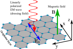
To describe the magnetoelectronic properties of dressed graphene, we have to solve the Schrödinger problem for electrons in a graphene layer exposed to both an electromagnetic wave (dressing field) and a stationary magnetic field (see Fig. 1).
Generally, electronic states near the and points of the Brillouin zone of graphene (the Dirac points) can be described by eight-component wave functions written in a basis corresponding to two crystal sublattices of graphene, two electron valleys, and two orientations of electron spin CastroNeto_2009 . In the following, the intervalley mixing of electron states and spin effects will be beyond consideration. Therefore, the number of necessary wave-function components can be reduced to two. Within this conventional approximation, the Hamiltonian of electrons near the point of the Brillouin zone has the form
| (1) |
where is the electron velocity at the Dirac point, is the operator of electron momentum in the graphene layer, is the modulus of electron charge, is the vector potential of the linearly polarized electromagnetic wave propagating perpendicularly to the graphene plane, is the amplitude of electric field of the wave, is the wave frequency, is the vector potential of the stationary magnetic field, , which is assumed to be directed perpendicularly to the graphene layer, and is the vector of Pauli matrices written in the basis of two orthogonal electron states arisen from the two crystal sublattices of graphene CastroNeto_2009 . Formally, these two basis states, and , correspond to the two opposite orientations of the pseudospin along the -axis, .
Let us introduce the new two orthonormal states,
| (2) |
where is the dimensionless parameter describing the interaction between an electron in graphene and a dressing field. Since Eq. (2) defines the complete system of basis states of graphene at any time , one can seek solutions of the Schrödinger problem as
| (3) |
where is the electron radius-vector in the graphene plane. Substituting the wave function (3) into the Schrödinger equation with the Hamiltonian (1), , we arrive at the two differential equations,
| (4) | |||||
which describe the quantum dynamics of dressed electrons in the graphene layer. Applying the conventional Floquet theory of periodically driven quantum systems Zeldovich_67 ; Grifoni_98 ; Platero_04 to the wave function (3), we can rewrite it as , where the function periodically depends on time, , and is the quasi-energy of an electron. Since the quasi-energy (the energy of dressed electron) is the physical quantity which plays the same role in periodically driven quantum systems as an usual energy in stationary ones, the present analysis of the Schrödinger problem is aimed to find the energy spectrum of dressed electron, . Taking into account the periodicity of the function , one can seek the coefficients in Eq. (4) as a Fourier expansion,
| (5) |
Substituting the expansion (5) into the expression (4) and applying the Jacoby-Anger expansion, to transform the exponent in the right side, one can rewrite Eq. (4) as
| (6) | |||||
It should be noted that Eq. (6) still describes exactly the initial Schrödinger problem. Next we will make some approximations.
Let us assume that the wave frequency, , is far from resonant electron frequencies corresponding to electron transitions between the different Landau levels in graphene, and, therefore, the inter-level absorption of the wave by electrons is absent. Thus, the considered electron system is conservative. Next, we have to take into account that the expansion coefficients in Eq. (5), , are the quantum amplitudes of the absorption (emission) of photons by an electron. Since the considered nonresonant field can be neither absorbed nor emitted by an electron, the amplitudes are very small, . Assuming the zero-order Bessel function, , to be far from zero, the aforesaid leads to the estimation
| (7) |
where It follows from the inequality (7) that the main contribution to the sum in Eq. (6) arises from terms with , which describe the elastic interaction between an electron and the dressing field. Therefore, small terms with in Eq. (6) can be omitted. It should be noted that such a neglect of high-frequency nonresonant terms in Eq. (6) is physically identical to the rotating wave approximation (RWA) which is conventionally used to describe various quantum systems under periodical pumping (see, e.g., Refs. Cohen-Tannoudji_b98 ; Scully_b01 ). Within this approach, Eq. (6) turns into the equation
| (8) |
Formally, Eq. (8) can be treated as a stationary Schrödinger equation, , with the effective Hamiltonian
| (9) |
where is the pseudospinor with the two components, . Applying the unitary transformation, , to the Hamiltonian (9), we arrive at the transformed Hamiltonian, , which has the well-behaved form
| (10) |
where the quantities and should be treated as components of the velocity of dressed electron along the axes. It should be noted that the electron velocity along the polarization vector of the dressing field, , is not changed by the the dressing field, whereas the electron velocity in the perpendicular direction, , drastically depends on the field because of the Bessel-function factor.
If the magnetic field is absent, , the Hamiltonian (10) can be diagonalized trivially and results in the anisotropic energy spectrum of dressed electrons Kristinsson_16 ,
| (11) |
where is the electron wave vector in the graphene plane. If a graphene layer is exposed to the magnetic field, , the Hamiltonian (10) is mathematically identical to the known Hamiltonian of “bare” graphene subjected to the same magnetic field, where the velocity of “bare” electron, , should be replaced with the velocity of dressed electron, . As a consequence, the electron eigenenergies and eigenfunctions corresponding to the Landau levels in dressed graphene can be easily obtained from well-known those for “bare” graphene CastroNeto_2009 with the formal replacement, . Particularly, the energies of the Landau levels in dressed graphene read as
| (12) |
where is the cyclotron frequency of graphene, is the magnetic length, is the signum function, and is the number of Landau level in the conductivity band () and the valence band (). As expected, the energies (12) exactly coincides with those in “bare” graphene CastroNeto_2009 if the dressing field is absent (). To avoid misunderstandings, one should keep in mind that the present theory is elaborated under condition (7). Therefore, Eqs. (8)–(12) are relevant if the Bessel function, , is far from zero.
According to Eq. (12), the dressing field changes the distance between the Landau levels. Physically, this effect originates from the linear electron dispersion in graphene. Indeed, in conducting systems with the parabolic dispersion of electrons the Landau levels are stable against a dressing field: The dressing field shifts the Landau levels uniformly but does not change the distance between them Inoshita_00 . Therefore, the magnetoelectronic properties of graphene will be very sensitive to the dressing field in contrast to the case of usual conducting systems with the parabolic dispersion of electrons.
III Optical and transport effects
The field-induced modification of the Landau levels (12) will manifest itself in various magneto-optical and magneto-transport phenomena. For definiteness, we will focus the attention on the optical absorption and longitudinal conductivity of dressed graphene.
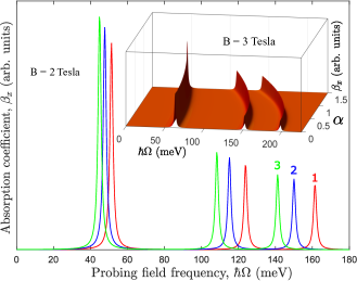
Let dressed graphene be subjected to a weak linearly polarized electromagnetic wave with the frequency (probing field). The probing field can induce electron transitions between the dressed Landau levels (12) which are accompanied by absorption of the field. Conventionally, this optical effect can be described by the absorption coefficient, . Combining the theory elaborated above and the known theory of magneto-optical absorption in “bare” graphene (see, e.g., Ref. Yao_13 ), we arrive at the expression for the absorption coefficient in dressed graphene,
| (13) |
where is the equilibrium filling factor for the Landau levels (12), are the resonance frequencies of dressed graphene corresponding to electron transitions between different Landau levels (12), is the decay rate at Landau levels which is assumed to be independent on the irradiation, is the scatterer-induced broadening of Landau levels, is the Kronecker symbol, and the index corresponds to the two polarizations of the probing field along the axes, respectively. The absorption coefficient (13) is plotted in Fig. 2 for various intensities of the dressing field, .
In order to analyze the longitudinal conductivity of dressed graphene in the presence of a magnetic field, let us use the conventional formalism based on the Kubo formula Ando_98 . Within this approach, the diagonal components of the conductivity tensor read as
| (14) |
with
| (15) |
where is the electron energy, is the Fermi distribution function, is the area of the graphene layer, is the operator of electron velocity along the axes, is the Green’s function of the effective Hamiltonian (10), and the broken brackets in Eq. (15) correspond to averaging over all possible configuration of random distributions of scatterers. Applying the conventional Green’s function technique within the self-consistent Born approximation, Shon and Ando calculated the conductivity of graphene for the cases of short-gange scatterers and long-range ones in the most general form Ando_98 . Particularly, they demonstrated that the self-energy is the same for the both kinds of scatterers. As to the vertex corrections, they vanish in the case of short-range scatterers but should be taken into account for long-range ones. In order to incorporate a dressing field into this known approach, we have to just replace the electron velocity in “bare” graphene, , with the velocity renormalized by the dressing field, , in the expression (15). It should be noted that the conductivity (15) can be calculated analytically in the important case of weak scattering, when the scatterer-induced broadeining of Landau levels, , is much less than the energy interval between nearest Landau levels. Taking into account the contribution of only Landau level at the Fermi energy and assuming the scattering processes in graphene to be caused by a long-range “white noise” disorder, we can write the conductivity (15) as
| (16) |
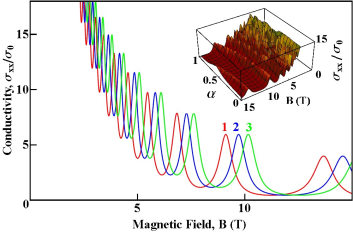
where is the conductivity of intrinsic graphene, and is the number of Landau level at the Fermi energy. As to the case of short-range disorder, it is described by the same expression (16) which should be just mupltiplied by the factor 2. As expected, the conductivity (16) exactly coincides with the known expression Ando_98 if a dressing field is absent (). The Shubnikov-de Haas oscillations of conductivity calculated within the approach Ando_98 for a graphene layer with short-range disorder are presented in Fig. 3 for various parameters of the dressing field.
IV Discussion and conclusions
Deriving the effective Hamiltonian (10), we assumed that the electromagnetic wave is nonresonant. This allowed us to neglect the inter-level absorbtion of the wave by electrons. However, we took also into account the scatterring-induced broadening of Landau levels, , where is the electron scattering time. For the self-consistency of the developed theory, we need to exclude the scattering-induced intra-level absorption of the wave by electrons within a broadened Landau level. Therefore, we have to assume the wave frequency, , to be high enough in order to satisfy the inequality . It is well-known that the nonresonant (collisional) absorption of wave energy by conduction electrons is negligibly small under this condition. Therefore, an electromagnetic wave which is both high-frequency and nonresonant can be treated as a purely dressing (nonabsorbable) field (see, e.g., Refs. Kibis_14 ; Morina_15 ; Pervishko_15 ). Such a purely dressing field should be used in experiments.
Physically, the absorption peaks in Fig. 2 correspond to the resonant electron transitions between dressed Landau levels, which are induced by a probing field. As to the Shubnikov-de Haas oscillations of the conductivity plotted in Fig. 3, their maxima correspond to the crossing of the Landau levels and the Fermi level. Since the distance between Landau levels (12) depends on a dressing field, the field-induced shifting of the maxima of the curves plotted in Figs. 2–3 appears. Besides the shifting, the dressing field leads to the anisotropy of magnetoelectronic properties caused by the nonequivalence of the electron velocities along the axes, . Namely, it follows from Eqs. (13) and (15) that . It should be noted that the discussed field-induced effects are most pronounced if the parameter of electron-field interaction, is large enough. Due to the giant electron velocity in graphene, m/s, this condition can be satisfied for relatively weak intensities of the dressing field (see Figs. 2–3). As a consequence, the optical and transport measurements are appropriate to detect the field-induced modification of electron energy spectrum (12) for experimentally reasonable parameters of the dressing field.
Physically, the considered features of the magnetoelectronic properties originate from the anisotropy of the energy spectrum of dressed electrons (11) along the axes. In turn, the anisotropy is caused by linear polarization of a dressing field. In the case of circularly polarized dressing field with the same electric field amplitude and frequency , the anisotropic spectrum (11) turns into the isotropic gapped one,
| (17) |
where is the field-induced gap Kibis_10 . Combining the theory of gapped graphene subjected to a magnetic field Koshino_10 and the theory of graphene layer dressed by a circularly polarized electromagnetic wave Kibis_10 , we easily arrive from the Hamiltonian (1) at the energy spectrum of Landau levels in the point of Brillouin zone,
| (18) |
where is the number of Landau level, and the upper and lower signs correspond to the conductivity and valence band, respectively. As to the Landau levels at the point, their structure can be also described by Eq. (18), where the signs “” under the square root should be replaced with the opposite signs, “”. It should be noted that the energy spectrum (18) is correct for weak magnetic fields satisfying the condition (for the opposite case of strong magnetic fields see Ref. Lopez_15 ). In contrast to Eq. (12), the energy spectrum (18) does not contain the Bessel function, . Mathematically, this means that the dependence of the magnetoelectronic properties of graphene on a dressing field is more pronounced in the case of linear polarization. Thus, a linearly polarized dressing field is preferable from experimental viewpoint.
As to experimental observability of the discussed effects, it should be noted that the employed parameters of the dressing field (the photon energy of meV scale and the field intensity of W/cm2) can be easily realized experimentally with using such conventional sources of THz radiation as quantum cascade lasers and free electron lasers (see, e.g., Refs. Williams_07 ; Carr_02 ).
Summarizing the aforesaid, we can conclude that a strong high-frequency electromagnetic field (dressing field) substantially modifies magnetoelectronic properties of graphene in contrast to the case of conventional conductors with the parabolic dispersion of electrons. Particularly, such resonant effects as optical absorption and Shubnikov-de Haas oscillations are very sensitive to the field. Therefore, a dressing field can be considered as a perspective tool to manipulate the magnetoelectronic properties of graphene. Since graphene serves as a basis for nanoelectronic devices, the developed theory opens a new way to control their characteristics.
V Acknowledgments
The work was partially supported by FP7 IRSES project QOCaN, FP7 ITN project NOTEDEV, Rannis project BOFEHYSS, Singaporean Ministry of Education under AcRF Tier 2 grant MOE2015-T2-1-055. OVK thanks RFBR project 14-02-00033 and Russian Ministry of Education and Science for the support. IAS thanks the Russian Target Federal Program “Research and Development in Priority Areas of Development of the Russian Scientific and Technological Complex for 2014-2020” of the Ministry of Education and Science of Russia (project 14.587.21.0020) for the support.
Appendix A Borders of applicability of the theory
In order to simplify comparison of the developed theory and experiments, we summarize the conditions of applicability of the theory:
(i) The dressing field is assumed to be off-resonant. Therefore, the frequency of the dressing field, , should be far from resonant frequencies corresponding to electron transitions between different Landau levels;
(ii) To exclude the scattering-induced intra-level absorption of the wave by electrons within a broadened Landau level, we have to assume the wave frequency, , to be high enough in order to satisfy the inequality . It is well-known that the nonresonant (collisional) absorption of wave energy by conduction electrons is negligibly small under this condition. Therefore, a dressing field which satisfies both the nonresonant condition (i) and the high-frequency condition (ii) can be treated as a purely dressing (non-absorbable) field;
(iii) The effective Hamiltonian (9) is derived by reducing the infinite system of quantum dynamics (6) to the sole equation (8). This reducing is correct under the condition , where is the Bessel function of the first kind, is the dimensionless parameter describing the interaction between an electron in graphene and a dressing field, is the electron velocity in graphene, is the amplitude of the dressing field, is the frequency of the dressing field, and . Thus, the dressing field amplitude, , and the field frequency, , should be chosen to keep the Bessel function, , far from zero;
References
- (1) K. S. Novoselov, A. K. Geim, S. V. Morozov, D. Jiang, Y. Zhang, S. V. Dubonos, I. V. Grigorieva, A. A. Firsov, Science 306, 666 (2004).
- (2) A. H. Castro Neto, F. Guinea, N. M. R. Peres, K. S. Novoselov, A. K. Geim, Rev. Mod. Phys. 81, 109 (2009).
- (3) S. Das Sarma, S. Adam, E. H. Hwang, E. Rossi, Rev. Mod. Phys. 83, 407 (2011).
- (4) M. O. Goerbig, Rev. Mod. Phys. 83, 1193 (2011).
- (5) C. H. Yang, F. M. Peeters, W. Xu, Phys. Rev. B 82, 075401 (2010).
- (6) A. Luican, G. Li, E. Y. Andrei, Phys. Rev. B 83, 041405 (2011).
- (7) F. Libisch, S. Rotter, J. Guttinger, C. Stampfer, J. Burgdorfer, Phys. Rev. B 81, 245411 (2010).
- (8) N. Gu, M. Rudner, A. Young, P. Kim, L. Levitov, Phys. Rev. Lett. 106 , 066601 (2011).
- (9) X. Yao, A. Belyanin, Phys. Rev. Lett. 108, 255503 (2012).
- (10) L. G. Booshehri, C. H. Mielke, D. G. Rickel, S. A. Crooker, Q. Zhang, L. Ren, E. H. Haroz, A. Rustagi, C. J. Stanton, Z. Jin, Z. Sun, Z. Yan, J. M. Tour, J. Kono, Phys. Rev. B 85, 205407 (2012).
- (11) I. Crassee, J. Levallois, A. L. Walter, M. Ostler, A. Bostwick, E. Rotenberg, T. Seyller, D. van der Marel, A. B. Kuzmenko, Nature Phys. 7, 48 (2011).
- (12) I. Crassee, M. Orlita, M. Potemski, A. L. Walter, M. Ostler, Th. Seyller, I. Gaponenko, J. Chen, A. B. Kuzmenko, Nano Lett. 12, 2470 (2012).
- (13) M. Grujic̀, M. Zarenia, A. Chaves, M. Tadic, G. A. Farias, F. M. Peeters, Phys. Rev. B 84, 205441 (2011).
- (14) R. Shimano, G. Yumoto, J. Y. Yoo, R. Matsunaga, S. Tanabe, H. Hibino, T. Morimoto , H. Aoki, Nature Commun. 4, 1841 (2013).
- (15) X. Yao, A. Belyanin, J. Phys: Condens. Matter 25 054203 (2013).
- (16) N. H. Shon, T. Ando, J. Phys. Soc. Japan 67, 2421 (1998).
- (17) F. Guinea, M. I. Katsnelson, A. K. Geim, Nature Phys. 6, 30 (2010) .
- (18) S. Das Sarma, S. Adam, E. H. Hwang, Enrico Rossi, Rev. Mod. Phys. 83, 407 (2011).
- (19) Z. Tan, C. Tan, L. Ma, G. T. Liu, L. Lu, C. L. Yang, Phys. Rev. B 84, 115429 (2011).
- (20) Z. Qiao, S. A. Yang, W. Feng, W. K. Tse, J. Ding, Y. Yao, J. Wang, Q. Niu, Phys. Rev. B 82, 161414 (2010).
- (21) J. Jobst, D. Waldmann, F. Speck, R. Hirner, D. K. Maude, T. Seyller, H. B. Weber, Phys. Rev. B 81, 195434 (2010).
- (22) D. Waldmann, J. Jobst, F. Speck, T. Seyller, M. Krieger, H. B. Weber, Nature Mater. 10, 357 (2011).
- (23) C. R. Dean, A. F. Young, P. Cadden-Zimansky, L. Wang, H. Ren, K. Watanabe, T. Taniguchi, P. Kim, J. Hone, K. L. Shepard, Nature Phys. 7 , 693 (2011).
- (24) C. Cohen-Tannoudji, J. Dupont-Roc, G. Grynberg, Atom-Photon Interactions: Basic Processes and Applications (Wiley, Chichester, 1998).
- (25) M. O. Scully, M. S. Zubairy, Quantum Optics (Cambridge University Press, Cambridge, 2001).
- (26) S. H. Autler, C. H. Townes, Phys. Rev. 100, 703 (1955).
- (27) S. P. Goreslavskii, V. F. Elesin, JETP Lett. 10, 316 (1969).
- (28) Q. T. Vu, H. Haug, O. D. Mücke, T. Tritschler, M. Wegener, G. Khitrova, H. M. Gibbs, Phys. Rev. Lett. 92, 217403 (2004).
- (29) Q. T. Vu, H. Haug, Phys. Rev. B 71, 035305 (2005).
- (30) A. Myzyrowicz, D. Hulin, A. Antonetti, A. Migus, W. T. Masselink, H. Morkoç, Phys. Rev. Lett. 56, 2748 (1986).
- (31) M. Wagner, H. Schneider, D. Stehr, S. Winnerl, A. M. Andrews, S. Schartner, G. Strasser, M. Helm, Phys. Rev. Lett. 105, 167401 (2010).
- (32) O. V. Kibis, Phys. Rev. B 86, 155108 (2012).
- (33) M. Teich, M. Wagner, H. Schneider, M. Helm, New J. Phys. 15, 065007 (2013).
- (34) O. V. Kibis, Europhys. Lett. 107, 57003 (2014).
- (35) S. Morina, O. V. Kibis, A. A. Pervishko, I. A. Shelykh, Phys. Rev. B 91, 155312 (2015).
- (36) A. A. Pervishko, O. V. Kibis, S. Morina, I. A. Shelykh, Phys. Rev. B 92, 205403 (2015).
- (37) O. V. Kibis, Phys. Rev. Lett. 107, 106802 (2011).
- (38) O. V. Kibis, O. Kyriienko, I. A. Shelykh, Phys. Rev. B 87, 245437 (2013).
- (39) F. K. Joibari, Y. M. Blanter, G. E. W. Bauer, Phys. Rev. B 90, 155301 (2014).
- (40) G. Yu. Kryuchkyan, O. Kyriienko, I. A. Shelykh, J. Phys. B 48, 025401 (2015).
- (41) F. J. López-Rodríguez, G. G. Naumis, Phys. Rev. B 78, 201406(R) (2008).
- (42) T. Oka and H. Aoki, Phys. Rev. B79, 081406(R) (2009).
- (43) T. Kitagawa, T. Oka, A. Brataas, L. Fu, E. Demler, Phys. Rev. B 84, 235108 (2011).
- (44) O. V. Kibis, Phys. Rev. B 81, 165433 (2010).
- (45) O. V. Kibis, O. Kyriienko, I. A. Shelykh, Phys. Rev. B 84, 195413 (2011).
- (46) G. Usaj, P. M. Perez-Piskunow, L. E. F. Foa Torres, C. A. Balseiro, Phys. Rev. B 90, 115423 (2014).
- (47) M. M. Glazov, S. D. Ganichev, Phys. Rep. 535, 101 (2014).
- (48) A. López, A. Di Teodoro, J. Schliemann, B. Berche, B. Santos, Phys. Rev. B 92, 235411 (2015).
- (49) Ya. B. Zel’dovich, Sov. Phys. JETP 24, 1006 (1967).
- (50) M. Grifoni, P. Hänggi, Phys. Rep. 304, 229 (1998).
- (51) G. Platero, R. Aguado, Phys. Rep. 395, 1 (2004).
- (52) K. Kristinsson, O. V. Kibis, S. Morina, I. A. Shelykh, Sci. Rep. 6, 20082 (2016).
- (53) T. Inoshita, Phys. Rev. B 61, 15610 (2000).
- (54) M. Koshino, T. Ando, Phys. Rev. B 81, 195431 (2010).
- (55) B. S. Williams, Nature Photonics 1, 517 (2007).
- (56) G. L. Carr, M. C. Martin, W. R. McKinney, K. Jordan, G. R. Neil, G. P. Williams, Nature 420, 153 (2002).