Solvababe supersymmetric algebraic model for descriptions of transitional even and odd mass nuclei near the critical point of the spherical to unstable shapes

Abstract

Exactly solvable solution for the spherical to gamma - unstable transition in transitional nuclei based on dual algebraic structure and nuclear supersymmetry concept is proposed. The duality relations between the unitary and quasispin algebraic structures for the boson and fermion systems are extended to mixed boson-fermion system. It is shown that the relation between the even-even and odd-A neighbors implied by nuclear supersymmetry in addition to dynamical symmetry limits can be also used for transitional regions. The experimental evidences are presented for even- even [E(5)] and odd-mass [E(5/4)] nuclei near the critical point symmetry.

Exactly solvable models play a key role in understanding some many - body problems in nuclear physics. A model may be solvable if its energy levels can be determined analytically and eigenstates are identified completely by the quantum numbers of a subgroup chain1 ; 2 . There are some many-body problems in nuclear physics that are exactly solvable, for example, three limits of dynamical symmetry of the interacting boson model2 . The IBM describes even-even nuclei in terms of correlated pairs of nucleons with L = 0, 2 treated as bosons (s, d bosons)3 . The N-boson system space is spanned by the irrep $\mathrm{[N]}$ of $\mathrm{U^{B}(6)}$ 3 . The interacting boson - fermion model also explains odd-A nuclei in terms of correlated pairs, s and d bosons , and unpaired particles of angular momentum j (j fermions)4 . The states of the boson - fermion system can be classified according to the irreducible representation $\mathrm{[N]\times[1]}$ of $\mathrm{U^{B}(6)\times U^{F}(M)}$ where M is the dimension of the single particle space. The IBM and IBFM can be unified into a supersymmetry (SUSY) approach that was discovered into nuclear structure physics in the early 1980 5 ; 6 . The experiments performed at various laboratories have confirmed the predictions made using a SUSY scheme 7 . Originally, nuclear supersymmetry was considered as symmetry among pairs of nuclei consisting of an even-even and an odd-even nuclei5 ; 6 . The supersymmetric representations $[\mathcal{N}\}$ of $\mathrm{U(6/M)}$ spanned a space explaining the lowest states of an even-even nucleus with $\mathcal{N}$ bosons and an odd-A nucleus with $\mathcal{N}-1$ bosons and an unpaired fermion4 . The nuclear supersymmetry has been used successfully in description of the dynamical symmetry limits of the even-even and odd-A nuclei4 ; 5 ; 6 . Virtually simultaneously, with the introduction of the nuclear supersymmetry, the idea of spherical-deformed phase transitions at low energy in finite nuclei germinated8 ; 9 . Studies of QPTs in odd-even nuclei with supersymmetric scheme had implicitly been initiated years before by A. Frank et al.10 . They have studied successfully a combination of $\mathrm{U^{BF}(5)}$ and $\mathrm{SO^{BF}(6)}$ symmetry by using $\mathrm{U(6/12)}$ supersymmetry for the Ru and Rh isotopes. Iachello 11 extended the concept of critical symmetry to critical supersymmetry and provided a benchmark for the study of shape phase transition in odd-even nuclei and also J.Jolie et al.12 studied QPTs in odd-even nuclei using a supersymmetric approach in interacting Boson-Fermion model.

The purpose of this letter is to point out that we have proposed a new solvable model for describing QPT for even and odd mass nuclei by using supersymmetry approach. In this paper, concept of supersymmetry and phase transitions are brought together by using the generalized quasi-spin algebra and Richardson - Gaudin method. We consider the state of fermions with spin j=3/2 coupled to boson core, however, our method is applicable for the whole systems with other values of spin of the fermions, j. In order to obtaining an algebraic solution for transitional region, we have used of dual algebraic structures. The duality symmetries are a powerful tool in relating the Hamiltonians with the number-conserving unitary and number-nonconserving quasi-spin algebras for system with pairing interactions13 ; 14 . These relations are obtained for both bosonic and fermionic systems13 ; 14 . We have established the duality relations for mixed boson-fermion system. In this paper, we display that the relation between the even-even and odd-A neighbors implied by nuclear supersymmetry in addition to dynamical-symmetry limits can also be used for transitional regions. So, the testing SUSY in all nuclear regions( dynamical symmetry limits and transitional region ) are possible. We investigate the change in level structure induced by the phase transition by doing a quantal analysis. The experimental evidences are presented for even- even [E(5)] and odd-mass [E(5/4)] nuclei near the critical point symmetry.

Details of the group theoretical description will be omitted from this paper and will be given in a subsequent detailed publication. The quasi-spin algebras have been explained in detail in Refs 13 ; 15 . The generalized quasi-spin algebra contains both bosonic (B) and fermionic (F) operators defined as 16

$$S_{BF}^{0}=\frac{1}{2}(n_{b}+n_{f})+\frac{1}{4}(N-M)$$ (1)

$$S_{BF}^{+}=\frac{1}{2}\sum\limits_{m}(-1)^{2\mp m}b_{m}^{+}b_{-m}^{+}\mp\frac{1}{2}\sum\limits_{m^{\prime}}(-1)^{j\mp m^{\prime}}a_{jm^{\prime}}^{+}a_{j-m^{\prime}}^{+}=\frac{1}{2}(b^{+}\cdot b^{+})\mp(a_{j}^{+}\cdot a_{j}^{+})$$ (2)

$$S_{BF}^{-}=\frac{1}{2}(\widetilde{b}.\widetilde{b})\pm\frac{1}{2}(\widetilde{a}_{j}.\widetilde{a}_{j})$$ (3)

Where $\mathrm{n_{b}}$ and $\mathrm{n_{f}}$are the boson and fermion number operators, respectively.Thus the operators $\mathrm{(S_{BF}^{\pm}}$,$\mathrm{S_{BF}^{0})}$ form a generalization of the usual fermionic and bosonic quasi-spin algebras with commutation relations given as 16

$$[S_{BF}^{0},S_{BF}^{\pm}]=\pm S_{BF}^{\pm}\quad,\quad[S_{BF}^{+},S_{BF}^{-}]=-2S_{BF}^{0}$$ (4)

The bosonic quasi-spin operators satisfy the commutation relations of the quasi-spin SU(1,1) algebra 13 ; 15 ; 16 while the fermionic quasi-spin operators satisfy the commutation relations of the quasi-spin SU(2) algebra 13 ; 15 ; 16 . The irreps of generalized quasi-spin algebra (GQA) are given in terms of the eigenvalues of the quadratic Casimir invariant and the quasi-spin operator $\mathrm{S_{BF}^{0}}$. The basis states of an irreducible representation (irrep)GQA, $\mathrm{|k,\mu\rangle}$ ,are determined by a single number $\mathrm{k}$ , susceptible of any positive number and $\mathrm{\mu=k,k+1,....}$ 16 Therefore,

$$|k,\mu\rangle=|\frac{N-M}{4}+\frac{\nu_{B}+\nu_{F}}{2},\frac{N-M}{4}+\frac{N_{B}+N_{F}}{2}\rangle$$ (5)

The basis states are determined considering the fact that fermionic part of the action of $\mathrm{S_{BF}^{+}}$ is restricted by the Pauli Exclusion Principle and the action of $\mathrm{S_{BF}^{-}}$ terminates when a state of $\mathrm{\nu}$ unpaired particles is reached i.e $\mathrm{S_{BF}^{-}|\nu_{B},\nu_{F}\rangle=0}$16 . In order to investigation the phase transition in atomic nuclei according to IBM, we have considered two kinds of bosons with L = 0, 2 (s, d bosons)3 . The generators of $\mathrm{SU^{d}(1,1)}$ and $\mathrm{SU^{s}(1,1)}$ are designated by considering and putting s and d operators only in the left part of Eqs.[1-3]and $\mathrm{SU^{sd}(1,1)}$ that is the s and d boson pairing algebras generated by 15

$$S^{+}(sd)=\frac{1}{2}(d^{+}.d^{+}\pm s^{+^{2}})\quad,\quad S^{-}(sd)=\frac{1}{2}(\widetilde{d}.\widetilde{d}\pm s^{2})\quad,S^{0}(sd)=\frac{1}{4}{\sum_{\nu}({d_{\nu}^{+}d_{\nu}+d_{\nu}d_{\nu}^{+}})}+\frac{1}{4}(s^{+}s+ss^{+})$$ (6)

Because of the duality relationships 13 ; 14 ; 15 , it is known that in even - even nuclei the base of $\mathrm{U(5)\supset SO(5)}$ and $\mathrm{SO(6)\supset SO(5)}$ are simultaneously the basis of $\mathrm{SU^{d}(1,1)\supset U(1)}$ and $\mathrm{SU^{sd}(1,1)\supset U(1)}$, respectively. By the use of duality relations 13 ; 15 , the Casimir operators of SO(5) and SO(6) can also be expressed in terms of the Casimir operators of $\mathrm{SU^{d}(1,1)}$ and $\mathrm{SU^{sd}(1,1)}$, respectively

$$\hat{C}_{2}(SU^{d}(1,1))=\frac{5}{16}+\frac{1}{4}\hat{C}_{2}(SO^{B}(5))$$ (7)

$$\hat{C}_{2}(SU^{sd}(1,1))=\frac{3}{4}+\frac{1}{4}\hat{C}_{2}(SO^{B}(6))$$ (8)

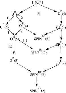
Figure 1: The lattice of algebras in the U(6/4) supersymmetry scheme.

The correspondence between the basis vectors in this case was shown in Ref.[15]. For a mixed boson-fermion system, the chain of subalgebras of unitary superalgebras U(6/M ) for j=3/2 is shown in Fig.1 and also two-level pairing system has two dynamical symmetries defined with respect to the generalized quasispin algebras, corresponding to either the upper or lower subalgebra chains in Eq.(9).

$$GQA_{1}^{sf}\otimes GQA_{2}^{df}\supset\left\{\begin{array}[]{cl}GQA_{1,2}^{sdf}\\ U_{1}^{sf}(1)\otimes U_{2}^{df}(1)\\ \end{array}\right\}\supset U_{1,2}^{sdf}$$ (9)

The upper subalgebra chain is corresponding to strong-coupling dynamical symmetry limit while lower chain is weak-coupling limit. Therefore, for odd-A nuclei, we have obtained the dual relation between the Casimir operators $\mathrm{Spin^{BF}(5)}$ and $\mathrm{GQA^{df}}$ (generalized quasispin algebra of d bosons and single fermion with j=3/2) as

If $\tau_{1}=v_{d}-\frac{1}{2}$ and $\tau_{2}=\frac{1}{2}$

$$\hat{C}_{2}(GQA^{df})=\frac{1}{4}\hat{C}_{2}(Spin^{BF}(5))-\frac{1}{4}(\tau_{1}+\frac{3}{4})$$ (10)

If $\tau_{1}=v_{d}+\frac{1}{2}$ and $\tau_{2}=\frac{1}{2}$

$$\hat{C}_{2}(GQA^{df})=\frac{1}{4}\hat{C}_{2}(Spin^{BF}(5))-\frac{1}{4}(3\tau_{1}+\frac{7}{4})$$ (11)

By the use of duality relations, the correspondence between the basis vectors $\mathrm{Spin^{BF}(5)}$ and $\mathrm{GQA^{df}}$ is

$$|\mathcal{N};[N_{B}=N],{N_{F}=1},\nu_{d},(\tau_{1}=v_{d}-\frac{1}{2},\tau_{2}),n_{\Delta}JM\rangle=|\mathcal{N};k^{d}=\frac{1}{2}(\nu_{d}+\frac{5}{2}),k^{df}=\frac{\tau_{1}+2}{2},\mu^{df}=\frac{1}{4}+\frac{1}{2}(n_{d}+n_{f}),n_{\Delta}JM\rangle$$ (12)

$$|\mathcal{N};[N_{B}=N],{N_{F}=1},\nu_{d},(\tau_{1}=v_{d}+\frac{1}{2},\tau_{2}),n_{\Delta}JM\rangle=|\mathcal{N};k^{d}=\frac{1}{2}(\nu_{d}+\frac{5}{2}),k^{df}=\frac{1+\tau_{1}}{2},\mu^{df}=\frac{1}{4}+\frac{1}{2}(n_{d}+n_{f}),n_{\Delta}JM\rangle$$ (13)

The Casimir operator of $\mathrm{Spin^{BF}(6)}$ and $\mathrm{GQA^{sdf}}$ (generalized quasispin algebra of d and s bosons with fermion j=3/2 ) has the following correspondence

If $\mathrm{\sigma_{1}=\sigma-\frac{1}{2}}$ and $\mathrm{\sigma_{2}=|\sigma_{3}|=\frac{1}{2}}$

$$\hat{C}_{2}(GQA^{sdf})=\frac{1}{4}\hat{C}_{2}(Spin^{BF}(6))-\frac{3}{4}(\sigma_{1}+\frac{3}{4})$$ (14)

If $\mathrm{\sigma_{1}=\sigma+\frac{1}{2}}$ and $\mathrm{\sigma_{2}=|\sigma_{3}|=\frac{1}{2}}$

$$\hat{C}_{2}(GQA^{sdf})=\frac{1}{4}\hat{C}_{2}(Spin^{BF}(6))-\frac{1}{4}(\sigma_{1}+\frac{3}{2})$$ (15)

By use of duality relations, the correspondence between the basis vectors $\mathrm{Spin^{BF}(6)}$ and $\mathrm{GQA^{sdf}}$ is

$$|\mathcal{N};[N_{B}=N],{N_{F}=1},\sigma,(\sigma_{1},\sigma_{2},\sigma_{3}),(\tau_{1},\tau_{2}),n_{\Delta}JM\rangle=|\mathcal{N};k^{sdf}=\frac{1}{2}(\sigma_{1}+\frac{3}{2}),\mu^{sdf}=\frac{1}{4}+\frac{1}{2}(n_{s}+n_{d}+n_{f}),n_{\Delta}JM\rangle$$ (16)

$$|\mathcal{N};[N_{B}=N],{N_{F}=1},\sigma,(\sigma_{1},\sigma_{2},\sigma_{3}),(\tau_{1},\tau_{2}),n_{\Delta}JM\rangle=|\mathcal{N};k^{sdf}=\frac{1}{2}(\sigma_{1}+\frac{5}{2}),\mu^{sdf}=\frac{1}{4}+\frac{1}{2}(n_{s}+n_{d}+n_{f}),n_{\Delta}JM\rangle$$ (17)

These relations have been used to effect simplifications of the calculations for two-level and multi-level systems13 . The infinite dimensional generalized quasispin algebra is generated by the use of 15

$$S_{BF,n}^{\pm}=c_{s}^{2n+1}S_{B}^{\pm}(s)+c_{d}^{2n+1}S_{B}^{\pm}(d)+c_{f}^{2n+1}S_{F}^{\pm}(f)$$ (18)

$$S_{BF,n}^{0}=c_{s}^{2n}S_{B}^{0}(s)+c_{d}^{2n}S_{B}^{0}(d)+c_{f}^{2n}S_{F}^{0}(f)$$ (19)

Where $\mathrm{c_{s}}$ ,$\mathrm{c_{d}}$ and $\mathrm{c_{f}}$ are real parameters and n can be $\mathrm{0,\pm 1,\pm 2,....}$. These generators satisfy the commutation relations

$$[S_{BF,m}^{0},S_{BF,n}^{\pm}]=\pm S_{BF,m+n}^{\pm}\quad\quad,\quad\quad[S_{BF,m}^{+},S_{BF,n}^{-}]=-2S_{BF,m+n+1}^{0}$$ (20)

Then,$\mathrm{{S_{BF,m}^{\mu},\mu=0,+,-;m=\pm 1,\pm 2,...}}$generate an affine generalized quasispin algebra $\mathrm{\widehat{GQA}}$ without central extension. The detailed description of the $\mathrm{U(6/4)}$ Supersymmetry in U(5) and O(6) limits can be found in 4 . By employing the generators of $\mathrm{\widehat{GQA}}$ and Casimir operators of subalgebras, the following Hamiltonian for transitional region between U(5)-O(6) limits is prepared

$$\hat{H}=S_{BF,0}^{+}S_{BF,0}^{-}+\alpha S_{BF,1}^{0}+\beta\hat{C}_{2}(Spin^{BF}(5))+\gamma\hat{C}_{2}(spin^{BF}(3))$$ (21)

It can be shown that Hamiltonian Eq.(21) is equivalent to a boson Hamiltonian for the even-even nuclei if acting on the $\mathrm{[N]\times[0]}$ representation of $\mathrm{U^{B}(6)\times U^{F}(4)}$ and with boson-fermion Hamiltonian for odd-A nuclei if acting on the $\mathrm{[N]\times[1]}$ representation of $\mathrm{U^{B}(6)\times U^{F}(4)}$. In odd-A nuclei, Hamiltonian Eq.(21) is equivalent to $\mathrm{O^{BF}(6)}$ Hamiltonian when $\mathrm{c_{s}=c_{d}=c_{f}}$ and with $\mathrm{U^{BF}(5)}$ Hamiltonian if $\mathrm{c_{s}=0}$ and $\mathrm{c_{d}\neq c_{f}\neq 0}$. So, the $\mathrm{c_{s}\neq c_{d}\neq c_{f}\neq 0}$ situation just corresponds to $\mathrm{U^{BF}(5)\leftrightarrow O^{BF}(6)}$ transitional region. Hamiltonian Eq.(21) in even-even nuclei is equivalent to $\mathrm{O(6)}$ Hamiltonian when $\mathrm{c_{s}=c_{d}}$ and with $\mathrm{U(5)}$ Hamiltonian if $\mathrm{c_{s}=0}$ and $\mathrm{c_{d}\neq 0}$ and Hamiltonian in transitional region with $\mathrm{c_{s}\neq c_{d}\neq 0}$. In our calculation, we take $\mathrm{c_{d}(=1)}$ constant value and $\mathrm{c_{s}}$ and $\mathrm{c_{f}}$ change between 0 and $\mathrm{c_{d}}$.

For evaluating the eigenvalues of Hamiltonian Eq.(21) the eigenstates are considered as

$$|k;\nu_{s}\nu n_{\Delta}LM\rangle=\textit{N}S_{BF}^{+}(x_{1})S_{BF}^{+}(x_{2})S_{BF}^{+}(x_{3})...S_{BF}^{+}(x_{k})|lw\rangle^{BF}$$ (22)

$$S_{x_{i}}^{+}=\frac{c_{s}}{1-c_{s}^{2}x_{i}}S_{B}^{+}(s)+\frac{c_{d}}{1-c_{d}^{2}x_{i}}S_{B}^{+}(d)+\frac{c_{f}}{1-c_{f}^{2}x_{i}}S_{F}^{+}(f)$$ (23)

The lowest weight state, $\mathrm{|lw\rangle^{BF}}$ , is defined as

$$|lw\rangle^{BF} =|\mathcal{N}=N_{B}+N_{F},k_{d}=\frac{1}{2}(\nu_{d}+\frac{5}{2}),\mu_{d}=\frac{1}{2}(n_{d}+\frac{5}{2}),k_{s}=\frac{1}{2}(\nu_{s}+\frac{1}{2}),\mu_{s}=\frac{1}{2}(n_{s}+\frac{1}{2}),k_{f}=\frac{1}{2}$$

$$(\nu_{f}-\frac{2j+1}{2}),\mu_{f}=\frac{1}{2}(n_{f}-\frac{2j+1}{2}),J,M\rangle$$ (24)

$$S_{n}^{0}|lw\rangle^{BF}=\Lambda_{n}^{0}|lw\rangle^{BF}\quad,\quad\Lambda_{n}^{0}=c_{s}^{2n}(\nu_{s}+\frac{1}{2})\frac{1}{2}+c_{d}^{2n}(\nu_{d}+\frac{5}{2})\frac{1}{2}+c_{f}^{2n}(\nu_{f}-\frac{2j+1}{2})\frac{1}{2}$$ (25)

The eigenvalues of Hamiltonian Eq.(21) can then be expressed as

$$E^{(k)}=h^{(k)}+\alpha\Lambda_{1}^{0}+\beta(\tau_{1}(\tau_{1}+3)+\tau_{2}(\tau_{2}+1))+\gamma J(J+1)\quad,\quad h^{(k)}=\sum_{i=1}^{k}{\frac{\alpha}{x_{i}}}$$ (26)

In order to obtain the numerical results for energy spectra $\mathrm{(E^{(k)})}$ of the considered nuclei, a set of non-linear Bethe-ansatz equations (BAE) with k- unknowns for k-pair excitations must be solved. Also constants of Hamiltonian with the least square fitting processes to experimental data are obtained. To achieve this aim, we have changed variables as

$$\mathrm{C_{s}=\frac{c_{s}}{c_{d}}\leq 1,C_{f}=\frac{c_{f}}{c_{d}}\leq 1,y_{i}=c_{d}^{2}x_{i}}$$

$$\frac{\alpha}{y_{i}}=\frac{C_{s}^{2}(\nu_{s}+\frac{1}{2})}{1-C_{s}^{2}y_{i}}+\frac{(\nu_{d}+\frac{5}{2})}{1-y_{i}}+\frac{C_{f}^{2}(\nu_{f}-\frac{2j+1}{2})}{1-C_{f}^{2}y_{i}}-{\sum_{j\neq i}{\frac{2}{y_{i}-y_{j}}}}$$ (27)

The quantum number $\mathrm{(k)}$ is related to $\mathrm{\mathcal{N}}$ by $\mathrm{\mathcal{N}=2k+\nu_{s}+\nu_{d}+\nu_{f}}$. The quality of the fits is specified by the values of $\mathrm{\sigma=(\frac{1}{N_{tot}}\sum_{i,tot}{|E_{exp}(i)-E_{Cal}(i)|^{2}})^{\frac{1}{2}}}$(keV) and $\mathrm{\phi=\frac{\sum\limits_{i}|E_{i}^{theor}-E_{i}^{exp}|}{\sum\limits_{i}E_{i}^{exp}}}$ (%) ($\mathrm{N_{tot}}$ the number of energy levels where included in the fitting processes)4 ; 15 .

The complete study of the properties of quantum phase transitions comprises both the classical and quantal analyses. In this study, we focus only on the quantal analysis and present the calculated phase transition observables such as the level crossing, the expectation value of the d-boson number operator and the expectation value of the fermion number operator.

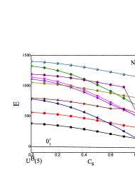
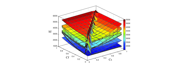
Figure 2: Energy levels as a function of $\mathrm{C_{s}}$ control parameter for a even-even nuclei (left panel) and for odd-A nuclei as a function of the $\mathrm{C_{s}}$ and $\mathrm{C_{f}}$ control parameters(right panel) in the Hamiltonian (20) for N=10 bosons with$\mathrm{\alpha=1000}$keV,$\mathrm{\beta=-1.29}$keV,$\mathrm{\gamma=6.05}$keV.

Once the eigenvalues have been obtained, we can display how the energy levels change within the whole range of the $\mathrm{C_{s}}$ and $\mathrm{C_{f}}$ control parameters. Fig.2 shows the energy surfaces of Hamiltonian of Eq.(21) for the neighboring even-even (left panel) and odd-A nuclei (right panel). The calculations are performed by considering the same fit parameters for these nuclei,where the parameters are $\mathrm{\alpha=1000}$keV, $\mathrm{\beta=-1.29}$keV, $\mathrm{\gamma=6.05}$keV, N=10 . Fig.2 shows how the energy levels as a function of the control parameter $\mathrm{C_{s}}$ and $\mathrm{C_{f}}$ evolve from one dynamical symmetry limit to the other . It can be seen from Figs that numerous level crossings occur. The crossings are due to the fact that $\mathrm{\nu_{d}}$, $\mathrm{O(5)}$ quantum number called seniority, is preserved along the whole path between O(6) and U(5) 12 ; 17 .

The other quantal order parameters that we consider here are the expectation values of the d-boson number operator and the expectation values of the fermion number operator.The expectation values of the d-boson number operator and fermion number operator are obtained as

$$\langle\hat{n_{d}}\rangle=\frac{\langle\psi|\hat{n_{d}}|\psi\rangle}{N}=\frac{2C_{s}^{2}C_{f}^{2}(\Lambda_{0}^{0}+k)-2(C_{s}^{2}+C_{f}^{2})(\Lambda_{1}^{0}+ky_{1}^{-1})+2(\Lambda_{2}^{0}+ky_{2}^{-2})}{N(1-C_{s}^{2})(1-C_{f}^{2})}-\frac{5}{2N}$$ (28)

$$\langle\hat{n_{f}}\rangle=\frac{\langle\psi|\hat{n_{f}}|\psi\rangle}{N}=\frac{2(1+C_{s}^{2})(\Lambda_{0}^{0}-\Lambda_{1}^{0}+k(1-y_{1}^{-1}))-2(\Lambda_{0}^{0}-\Lambda_{2}^{0}+k(1-y_{2}^{-2}))}{N(1-C_{f}^{2})(C_{s}^{2}-C_{f}^{2})}+\frac{2j+1}{2N}$$ (29)

Fig.3 shows the expectation values of the d-boson number operator for the lowest states even-even (left panel) and odd-A nuclei (right panel) as a function of control parameters for N=10 bosons. Fig.3 (left panel) displays that the expectation values of the number of d bosons for each L, $\mathrm{n_{d}}$, remain approximately constant for $\mathrm{C_{s}<0.45}$ and only begin to change rapidly for $\mathrm{C_{s}>0.45}$. The near constancy of $\mathrm{n_{d}}$ for $\mathrm{C_{s}<0.45}$, is an obvious indication that U(5) dynamical symmetry is preserved in this region to a high degree and also the $\mathrm{n_{d}}$ values change rapidly with $\mathrm{C_{s}}$ over the range $\mathrm{0.65\leq C_{s}\leq 1}$. Fig.4 shows likewise $\mathrm{\langle n_{f}\rangle}$ as a function of the $\mathrm{C_{s}}$ and $\mathrm{C_{f}}$ control parameters.

Nuclear physics has made important contributions to study QPTs because nuclei display a variety of phases in systems ranging from few to many particles 18 . The nuclei in the mass regions around 130 have transitional characteristics, intermediate between the spherical and gamma-unstable shapes19 . The calculations have been done along Xe and Ba isotopic chains exhibit that $\mathrm{{}^{134}Ba}$ and $\mathrm{{}^{130}Xe}$ are the best candidates E(5) critical point symmetry 19 ; 20 . The first Bose-Fermi critical symmetry, called E(5/4), has been proposed for an odd-A system in Ref.11 . A search for experimental examples of E(5/4) should concentrate on the case that a $j=3/2$ particle if coupled to an E(5) core, $\mathrm{{}^{135}Ba}$ and $\mathrm{{}^{131}Xe}$ built on the single particle neutron in the $\mathrm{2d_{\frac{3}{2}}}$ shell model orbit should be possible candidates 11 ; 19 ; 20 . In what follows we describe a simultaneous analysis of $\mathrm{{}^{134}Ba}$ with $\mathrm{{}^{135}Ba}$ and $\mathrm{{}^{130}Xe}$ with $\mathrm{{}^{131}Xe}$ within the U(6/4) supergroup. In order to obtain energy spectrum and realistic calculation for these nuclei, we need to specify Hamiltonian parameters Eq.(21). According to the supersymmetry concept, the even-even and odd-A nuclei are described by the same set of fit parameters, thus to achieve a better fit the states of both nuclei were used. The best fits for Hamiltonian’s parameters, namely $\mathrm{\alpha}$, $\mathrm{\beta}$ and $\mathrm{\gamma}$, used in the present work are shown in Table 1. A comparison between the available experimental levels and the predictions of our results for the $\mathrm{{}^{134-135}Ba}$ and $\mathrm{{}^{130-131}Xe}$ isotopes in the low-lying region of spectra along with $\mathrm{R_{\frac{4}{2}}=\frac{E(\nu_{d}=2)}{E(\nu_{d}=1)})}$ values are shown in Fig. 5 and Fig. 6, respectively.The $\mathrm{R_{\frac{4}{2}}}$ value is one of the most basic structural predictions of $\mathrm{U(5)-O(6)}$ transition19 ; 20 . The ratio equal to 2.2-2.3 indicates the spectrum of transitional nuclei19 ; 20 . We have tried to extract the best set of parameters which reproduce these complete spectra with minimum variations. It means that our suggestion to use this transitional Hamiltonian for the description of the Ba and Xe isotopes would not have any contradiction with other theoretical studies done with special hypotheses about mixing of intruder and normal configurations. So, we conclude from the values of control parameter which has been obtained and $\mathrm{R_{\frac{4}{2}}}$ value, that $\mathrm{{}_{56}^{134-135}Ba}$ and $\mathrm{{}_{54}^{130-131}Xe}$ isotopes are the best candidates for U(5)-O(6) transition in U(6/4) supersymmetry scheme.

Although, studies of QPTs in odd-even and even-even nuclei were extensively done, our results are novel, since (1) we have proposed exactly-solvable supersymmetry Richardson-Gaudin (R-G) model for transitional region by which we can be investigate the phase transition observables in the both of nuclei by using of the concept of supersymmetry (2) The experimental evidences have been presented for E(5) and E(5/4) nuclei and have been analyzed them by supersymmetry scheme. The important new result of the present paper is to have employed the nuclear supersymmetry approach for description of the transitional region between spherical and gamma -unstable phase shape in addition to dynamical symmetry limits in one chain isotopic.

Table 1. Parameters of Hamiltonian Eq.(20) used in the calculation of the Ba and Xe nuclei. All parameters are given in keV.

Nucleus	$\mathcal{N}$	$\mathrm{C_{s}}$	$\mathrm{C_{f}}$	$\mathrm{\alpha}$	$\mathrm{\beta}$	$\mathrm{\gamma}$	$\mathrm{\sigma}$	$\mathrm{\phi}$
$\mathrm{{}^{134}Ba-^{135}Ba}$	5	0.52	0.8	333.12	1.945	0.73	155.42	10.73%
$\mathrm{{}^{130}Xe-^{131}Xe}$	5	0.55	0.9	187.84	0.9564	10.98	143.29	12.4%

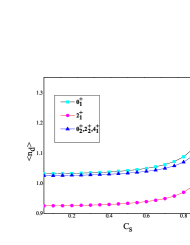
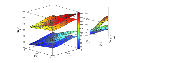
Figure 3: The expectation values of the d-boson number operator for the lowest states as a function of $\mathrm{C_{s}}$ control parameter for an even-even nuclei (left panel) and for odd-A nuclei as a function of the $\mathrm{C_{s}}$ and $\mathrm{C_{f}}$ control parameters(right panel).

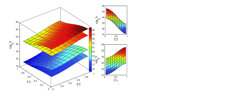
Figure 4: The expectation values of the fermion number operator for odd-A nuclei for the lowest states as a function of $\mathrm{C_{s}}$ and $\mathrm{C_{f}}$ control parameters.

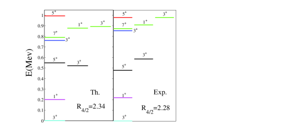
Figure 5: Comparison between calculated and experimental spectra of positive parity states in $\mathrm{{}^{134}Ba}$ (left panel) and $\mathrm{{}^{135}Ba}$(right panel) . The parameters of the calculation are given in Table 1. The experimental spectra, is taken from.21

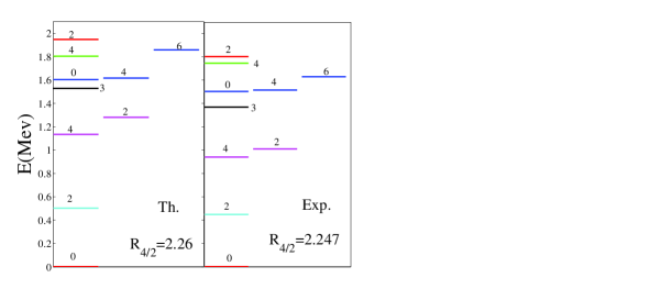
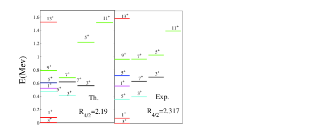
Figure 6: Comparison between calculated and experimental spectra of positive parity states in $\mathrm{{}^{130}Xe}$(top panel) and $\mathrm{{}^{131}Xe}$(bottom panel). The parameters of the calculation are given in Tables 1. The experimental spectra, is taken from.21

References

(1) D. J. Rowe, C. Bahri, and W. Wijesundera, Phys. Rev. Lett. 80, 4394 (1998).
(2) Feng Pan and J.P.Draayer, Annals of physics 271, 120-140 (1999).
(3) F. Iachello and A. Arima, The interacting boson model (Cambridge University Press, 1987).
(4) F. Iachello and P. Van Isacker, The interacting boson-fermion model (Cambridge University Press, 1991).
(5) F. Iachello, Phys. Rev. Lett. 44, 772 (1980).
(6) A. B. Balantekin, I. Bars, and F. Iachello, Phys. Rev. Lett.
47, 19 (1981); Nucl. Phys. A370, 284 (1981).
(7) A. Metz et al., Phys. Rev. Lett. 83, 1542 (1999); Phys.
Rev. C 61, 064313 (2000); J. Gro¨ger et al., Phys. Rev. C
62, 064304 (2000).
(8) F. Iachello, N. V. Zamfir, and R. F. Casten, Phys. Rev. Lett. 81,
1191 (1998).
(9) R. F. Casten, D. Kusnezov, and N. V. Zamfir, Phys. Rev. Lett.
82, 5000 (1999).
(10) A. Frank, P. Van Isacker and D.D. Warner, Phys. Lett. B 197, 474 (1987).
(11) F. Iachello, Physical review letters 95, 052503 (2005).
(12) J.Jolie, S. Heinze, P. Van Isacker, and RF.Casten, Phys. Rev. C 70, 011305(R)(2004).
(13) M. Caprio, J. Skrabacz, and F. Iachello, Journal of Physics A: Mathematical and Theoretical 44, 075303 (2011).
(14) D. Rowe, M. Carvalho, and J. Repka, Reviews of Modern Physics 84, 711 (2012).
(15) F. Pan and J. Draayer, Nuclear Physics A 636, 156 (1998).
(16) P.D.Jarvis, Mei Yang and B.G.Wybourne, Journal of Mathematical Physics 28,1192 (1987).
(17)P. Cejnar, S. Heinze, and J. Jolie, Phys. Rev. C 68, 034326
(2003).
(18) D. Rowe, Nuclear Physics A 745, 47 (2004).
(19) R. Casten and E. McCutchan, Journal of Physics G: Nuclear and Particle Physics 34, R285 (2007).
(20) M. Caprio and F. Iachello, Nuclear Physics A 781, 26 (2007).
(21) National nuclear data center, http://www.nndc.bnl.gov/chart/reColor.jspnewColor=dm.