Granger Causality in Multi-variate Time Series using a Time Ordered Restricted Vector Autoregressive Model

Abstract

Granger causality has been used for the investigation of the inter-dependence structure of the underlying systems of multi-variate time series. In particular, the direct causal effects are commonly estimated by the conditional Granger causality index (CGCI). In the presence of many observed variables and relatively short time series, CGCI may fail because it is based on vector autoregressive models (VAR) involving a large number of coefficients to be estimated. In this work, the VAR is restricted by a scheme that modifies the recently developed method of backward-in-time selection (BTS) of the lagged variables and the CGCI is combined with BTS. Further, the proposed approach is compared favorably to other restricted VAR representations, such as the top-down strategy, the bottom-up strategy, and the least absolute shrinkage and selection operator (LASSO), in terms of sensitivity and specificity of CGCI. This is shown by using simulations of linear and nonlinear, low and high-dimensional systems and different time series lengths. For nonlinear systems, CGCI from the restricted VAR representations are compared with analogous nonlinear causality indices. Further, CGCI in conjunction with BTS and other restricted VAR representations is applied to multi-channel scalp electroencephalogram (EEG) recordings of epileptic patients containing epileptiform discharges. CGCI on the restricted VAR, and BTS in particular, could track the changes in brain connectivity before, during and after epileptiform discharges, which was not possible using the full VAR representation.

I Introduction

Granger causality has been applied to reveal inter-dependence structure in multi-variate time series, first in econometrics [1, 2, 3], and then to other areas and in particular to neuroscience, e.g. see the special issue in [4]. According to the concept originally introduced by Granger [5], a variable $X$ Granger causes another variable $Y$ if the prediction of $Y$ is improved when $X$ is included in the prediction model for $Y$. In multi-variate time series, the other observed variables are included in the two vector autoregressive (VAR) models for $Y$. The model including $X$ is called unrestricted or U-model, whereas the one not including $X$ is called restricted or R-model. The Granger causality is quantified by the conditional Granger causality index (CGCI), defined as the logarithm of the ratio of the error variances of the R-model and the U-model (the term conditional stands for the general case of other observed variables included in the two models) [6, 7]. Apart from CGCI and its formulations in the frequency domain, i.e. the partial directed coherence [8] and the direct directed transfer function [9], a number of nonlinear Granger causality indices have been proposed based on information theory [10, 11], state space dynamics [12, 13] and phase synchronization [14] (for a comparison see [15, 16]). However, when inherently nonlinear and complex systems are studied at small time intervals the nonlinear methods are not successfully applicable [16]. The same may hold for the CGCI and other indices based on VAR models. In particular, the estimation of the VAR coefficients may be problematic in the setting of many observed variables and short time series.

The problem of reducing the number of model coefficients has been addressed in linear multiple regression, and many methods of variable subset selection have been developed. The optimal solution is obtained by the computationally intensive and often impractical search for all subset models. Suboptimal subset selection methods include the simple sequential search method and stepwise methods implementing the bottom-up (forward selection) and top-down (backward elimination) strategies. More complicated schemes have also been proposed, such as the genetic algorithms, the particle swarm optimization and the ant colony optimizations. The most popular methods seem to be the ridge regression and the least absolute shrinkage and selection operator (LASSO), as well as the combination of them, and other variants of LASSO [17, 18]. Other methods deal with dimension reduction through transformation and projection of the variable space, such as the principal component regression and the partial least squares regression, or assume a smaller set of latent variables, such as the dynamic factor models [19]. These latter methods are not considered here because the purpose is to identify the inter-dependence between the observed variables and not between transformed or latent variables. All the aforementioned methods are developed for regression problems and do not take into account the lag dependence structure that typically exists in multi-variate time series. This is addressed in a recently developed method known as backward-in-time-selection (BTS), which implements a supervised stepwise forward selection guided by the lag order of the lagged variables [20]. Starting the sequential selection from smallest to larger lags is reasonable as in time series problems it is expected that the variables at smaller lags are more explanatory to the response variable (at the present time) than variables at larger lags. Thus conditioning on the variables at smaller lags the variables at larger lags may only enter the model if they have genuine contribution not already contained in the selected variables of smaller lags. It is reasonable to expect that in time series problems the response (present) variable does not depend on all lagged variables, as implied in the standard VAR approach. So, dimension reduction may be useful in any case of multi-variate time series, not only for the case of high dimensional time series of short length, where VAR estimation fails.

So far there has been little focus on the problem of estimating the linear Granger causality index in short time series of many variables, where standard VAR model estimation may be problematic. We are aware only of works attempting to estimate Granger causality after restricting the VAR models using LASSO and variants of this [21, 22, 23, 24, 25] (for restricted VAR model using LASSO see also [26, 27, 28, 29]). There are also applications of LASSO in neuroscience, such as electroencephalograms [30] and fMRI [31, 32], and bioinformatics, in microarrays [33, 34].

In this work, we propose a new dimension reduction approach designed for time series. We modify and adapt the BTS method for Granger causality, and develop the scheme called BTS-CGCI that derives CGCI from the restricted VAR representation formed by BTS (BTS-CGCI). Further, we compare BTS-CGCI to the CGCI derived by other restricted VAR representations (top-down, bottom-up, LASSO) and the full VAR representation. The ability of the different VAR representations to identify the connectivity structure of the underlying system to the observed time series is assessed by means of Monte Carlo simulations. In the simulation study, we included known linear and nonlinear, low and high-dimensional systems, and considered different time series lengths. In particular, for nonlinear systems, the comparison includes also two nonlinear information based measures, i.e. the partial transfer entropy [35, 36], in analogy to CGCI from the full VAR representation, and the partial mutual information from mixed embedding (PMIME), in analogy to CGCI from the restricted VAR [11]. Moreover, BTS-CGCI along with other restricted and full VAR representations are applied to multi-channel scalp electroencephalogram (EEG) recordings of epileptic patients containing epileptiform discharges. The obtained brain network before, during and after epileptiform discharges, is assessed for each method.

The structure of the paper is as follows. In Section II, BTS-CGCI is presented along with other VAR restriction methods as well as their statistical evaluation. In Section III, the simulation study is described and the results are presented. The application to EEG is presented and discussed in Section IV. Finally, the method and results are discussed in Section V.

II Methods

II-A The conditional Granger causality index

Let $X_{t}=\{X_{1,t},X_{2,t},\ldots,X_{K,t}\}$, $t=1,\ldots,N$, be a $K$-dimensional stationary time series of length $N$. The definition of the conditional Granger causality index (CGCI) from a driving variable $X_{i}$ to a response variable $X_{j}$ involves two vector autoregressive (VAR) models for $X_{j}$, called also dynamic regression models [37]. The first model is the unrestricted model (U-model) [38], given as

$$X_{j,t}=\sum_{k=1}^{K}(a_{jk,1}X_{k,t-1}+\ldots+a_{jk,p}X_{k,t-p})+u_{j,t}$$ (1)

where $p$ is the model order and $a_{jk,l}$ ($k=1,\ldots,K$, $l=1,\ldots,p$) are the U-model coefficients. The U-model includes all the $K$ lagged variables for lags up to the order $p$. The second model is the restricted one (R-model) derived from the U-model by excluding the lags of $X_{i}$, given as

$$X_{j,t}=\sum_{k=1,k\neq i}^{K}(b_{jk,1}X_{k,t-1}+\ldots+b_{jk,p}X_{k,t-p})+e_{j,t}$$ (2)

where $b_{jk,l}$ ($k=1,\ldots,K$ but $k\neq i$ and $l=1,\ldots,p$) are the coefficients of the R-model. The terms $u_{j,t}$ and $e_{j,t}$ are white noise with mean zero and variances $\sigma^{2}_{U}$ and $\sigma^{2}_{R}$, respectively. Moreover, for inference (see the significance test below) they are assumed to have normal distribution. Fitting the U-model and R-model, typically with ordinary least squares (OLS), we get the estimates of the residual variances $\hat{\sigma}^{2}_{U}$ and $\hat{\sigma}^{2}_{R}$. Then CGCI from $X_{i}$ to $X_{j}$ is defined as

$$\mbox{CGCI}_{X_{i}\rightarrow X_{j}}=\ln\frac{\hat{\sigma}^{2}_{R}}{\hat{\sigma}^{2}_{U}}.$$ (3)

CGCI is at the zero level when $X_{i}$ does not improve the prediction of $X_{j}$ (the U-model and R-model give about the same fitting error variance) and obtains larger positive values when $X_{i}$ improves the prediction of $X_{j}$ indicating that $X_{i}$ Granger causes $X_{j}$.

The statistical significance of CGCI is commonly assessed by a parametric significance test on the coefficients of the lagged driving variable $X_{i}$ in the U-model [38]. The null hypothesis is H₀: $a_{ji,l}=0$ for all $l=1,\ldots,p$, and the Fisher statistic is

$$F=\frac{(\mbox{SSE}^{R}-\mbox{SSE}^{U})/p}{\mbox{SSE}^{U}/((N-p)-Kp)},$$ (4)

where SSE is the sum of squared errors and the superscript denotes the model, $N-p$ is the number of equations and $Kp$ is the number of coefficients of the U-model. The Fisher test assumes independence of observations, normality and equal variance for the observed variables, which may not be met in practice. We refrain from discussing these issues here as the test is commonly applied in the VAR based estimation of Granger causality, and only note that the assumption of independence is likely to be violated as the time series are typically auto- and cross- correlated. When there are many observed variables (large $K$) and short time series (small $N$), so that $Kp$ is large compared to $N$, the estimation of the model coefficients may not be accurate and then CGCI cannot be trusted.

II-B The modified backward in time selection

The backward-in-time-selection (BTS) method is a bottom-up strategy designed for multi-variate time series to reduce the terms in the VAR model in (1) [20]. The BTS method is developed so as to take into account feedback and multi-collinearity, which are often observed in multi-variate time series. The rationale is to select the order $p_{k}$ for each $X_{k}$ in the dynamic regression model in (1) (instead of having the same order $p$ for all variables) based on the inherent property of time series that the dependence structure is closely related to the temporal order of the variables. Thus BTS evaluates progressively the inclusion of the lagged variables in the model, starting with the most current lagged variables and moving backwards in time. While the model derived by the BTS method in [20] includes all lags up to the selected order $p_{k}$ for each $X_{k}$, here we modify the BTS method so as to include in the model only the lags of each $X_{k}$ that are selected at each step of the algorithm. The modified algorithm of BTS (mBTS) is briefly presented below (we use the notation mBTS for the modified algorithm but keep the notation BTS for the derived model and the Granger causality approach). We note that the algorithm described below is for determining one dynamic regression model for one of the $K$ variables, say $X_{j}$, and it is repeated $K$ times for all $K$ variables.

First, a maximum order $p_{\mbox{\footnotesize{max}}}$ is set determining the maximum lag the algorithm will search for all $K$ variables to add in the dynamic regression model for the response variable $X_{j}$. Thus the vector of all lagged variables that are candidates to be included in the BTS model is

$$\mathbf{W}=[X_{1,t-1}\ldots X_{1,t-p_{\mbox{\footnotesize{max}}}}X_{2,t-1}\ldots X_{K,t-p_{\mbox{\footnotesize{max}}}}],$$

and has $Kp_{\mbox{\footnotesize{max}}}$ components. The algorithm aims at finding an explanatory vector $\mathbf{w}_{j}$ formed from the the most significant lagged variables of $\mathbf{W}$ in predicting $X_{j}$, which thus comprise the BTS model. The explanatory vector $\mathbf{w}_{j}$ is built progressively adding one lagged variable at each cycle. The models formed by the candidate explanatory vectors at each cycle are assessed with the Bayesian information criterion (BIC) [39]. The steps of the mBTS algorithm are given below and the pseudo-code is given in Algorithm 1.

Algorithm 1 mBTS for $X_{j}$

1:$X$: The set of $K$ time series

2:$w\leftarrow\emptyset$ $\triangleright$ initially explanatory vector is empty

3:$\textit{BICold}\leftarrow s^{2}$ $\triangleright$ $s^{2}$: the error variance

4:$\textit{maxlags}\leftarrow[0,\ldots,0]$ $\triangleright$ the $K$ maximum lags are initially set to zero

5:while $\textit{sum(maxlags)}<K\textit{pmax}$ do

6:     for $i=1:K$ do

7:         if $\textit{maxlags}(i)<\textit{pmax}$ then

8:              $\textit{wcand}\leftarrow\{w;(i,\textit{maxlags}(i)+1)\}$

9:              $\textit{BIC}(i)\leftarrow\mbox{modelfit}(j,X,\textit{wcand})$

10:         else

11:              $\textit{BIC}(i)\leftarrow\textit{BICold}$               

12:     $[\textit{BICnew},k]\leftarrow\min(\textit{BIC})$ $\triangleright$ $k$ is the corresponding index to min

13:     if $\textit{BICnew}<\textit{BICold}$ then

14:         $\textit{BICold}\leftarrow\textit{BICnew}$

15:         $w\leftarrow\{w;(k,\textit{maxlags}(k)+1)\}$

16:         $\textit{maxlags}(k)\leftarrow\textit{maxlags}(k)+1$

17:     else

18:         for $i=1:K$ do

19:              $\textit{maxlags}(i)\leftarrow\min(\textit{maxlags}(i)+1,\textit{pmax})$               return $w$

1. Initially, let the explanatory vector of lagged variables $\mathbf{w}_{j}^{0}$ be empty, corresponding to the zero-order model and BIC here is equal to the variance of $X_{j}$ (lines 1-3 in the pseudo-code; ’maxlags’ is an auxiliary array keeping track of the maximum lag of each variable already searched, and therefore it is initially set to zero for each of the $K$ variables).

2. For each of the $K$ variables separately, its largest tested lag so far is increased by one and this lagged variable is added to the current explanatory vector $\mathbf{w}_{j}^{l}$ (the superscript denotes the size of the current explanatory vector). In this way, $K$ candidate explanatory vectors are formed. For the first cycle, the current explanatory vector $\mathbf{w}_{j}^{0}$ is empty and the $K$ candidate explanatory vectors are actually the $K$ scalar variables

   $$X_{1,t-1},\ldots,X_{K,t-1}.$$

   For the $l+1$ cycle, the explanatory vector $\mathbf{w}_{j}^{l}$ has $l$ lagged variables, and let the maximum lag for each variable $X_{k}$ in $\mathbf{w}_{j}^{l}$ be $\tau(l_{k})$ ($\tau(l_{k})$ is zero if $X_{k}$ is not yet present in $\mathbf{w}_{j}^{l}$). Then the $K$ candidate explanatory vectors are

   $$[\mathbf{w}_{j}^{l}\,\,X_{1,t-\tau(l_{1})-1}],\ldots,[\mathbf{w}_{j}^{l}\,\,X_{K,t-\tau(l_{K})-1}].$$

   Compute BIC for the $K$ dynamic regression models formed by the $K$ candidate explanatory vectors (lines 5-10 in the pseudo-code; the components of the candidate explanatory vector ’wcand’ are pairs of two numbers, the first indicating the variable and the second the lag; the function ’modelfit’ in line 8 provides the BIC value for the fitted model defined by ’wcand’).

3. Find the candidate explanatory vector for which the BIC value is smaller than the BIC value for $\mathbf{w}_{j}^{l}$. If there are more than one such vectors (models) select the one with the smallest BIC value. Update the current explanatory vector with the explanatory vector of smallest BIC, denoted $\mathbf{w}_{j}^{l+1}$ (lines 11-15 in the pseudo-code). The $l+1$ cycle is thus completed and go to the next step. If none of the $K$ candidate explanatory vectors gives BIC smaller than the one for $\mathbf{w}_{j}^{l}$, then increase the maximum lag $\tau(l_{k})$ for each $X_{k}$ by one and go to the next step (if $\tau(l_{k})=p_{\mbox{\footnotesize{max}}}$ for any $k=1,\ldots,K$, leave it as is; lines 16-18 in the pseudo-code).

4. If all the maximum lags reached the maximum order, $\tau(l_{k})=p_{\mbox{\footnotesize{max}}}$ ($k=1,\ldots,K$) then terminate, otherwise go to step 2 (line 4 in the pseudo-code).

Upon termination after $P_{j}$ cycles, the algorithm gives the final explanatory vector $\mathbf{w}_{j}$ of size $P_{j}$ for $X_{j}$. It is noted that $\mathbf{w}_{j}$ may not have lagged components of all $K$ variables. Moreover, if a variable $X_{k}$ is present in $\mathbf{w}_{j}$ with maximum lag $\tau(p_{k})$, $\mathbf{w}_{j}$ may not contain all lags of $X_{k}$ from one to $\tau(p_{k})$, but a subset of $p_{k}$ lags, and in general $p_{k}\leq\tau(p_{k})$ holds. The latter constitutes a modification to the original BTS algorithm in [20], where for each $X_{k}$ in $\mathbf{w}_{j}$ all lags up to the maximum lag $\tau(p_{k})$ are included in $\mathbf{w}_{j}$ and subsequently in the model for $X_{j}$. The reason for this modification is to include in the dynamic regression model for $X_{j}$ only terms (lagged variables) found to improve the prediction of $X_{j}$, and this allows for the identification of the exact lags of the variable that give evidence of Granger causality. On the other hand, the inclusion of all lags of a variable up to the selected order may possibly block the presence of specific lags of other variables, and this would reduce the sensitivity in detecting Granger causality effects.

The steps of mBTS are illustrated in Figure 1 for a simple example of the following VAR(4) system in two variables

$$X_{1,t} = 0.4X_{1,t-1}+u_{1,t}$$

$$X_{2,t} = 0.4X_{2,t-1}-0.3X_{1,t-4}+u_{2,t}$$ (5)

The explanatory vector $\mathbf{w}_{2}$ found by mBTS in Figure 1a is different than that found by BTS in Figure 1b. The explanatory vector by mBTS includes the two true lagged variables and one other lagged variable $X_{1,t-3}$ not included in the expression for $X_{2,t}$, which however does not result in wrong causal effects, while BTS includes also two more lagged variables, i.e. all lagged variables of $X_{1}$ up to order four.

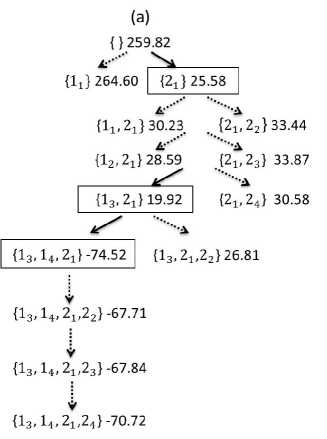
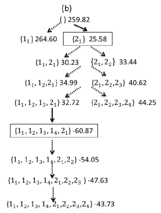
Figure 1: (a) The steps of the mBTS algorithm for the second response variable of the VAR(4) system in two variables. At each step the candidate explanatory vector is shown (the integer number indicates the variable and the subscript the lag) together with the corresponding BIC value. When a lagged variable is selected the vector and BIC value are shown in box and the arrow is given with solid line (dashed line otherwise). (b) The same for BTS.

II-C The conditional Granger causality index and backward-in-time selection

We propose to calculate $\mbox{CGCI}_{X_{i}\rightarrow X_{j}}$ making use of the mBTS algorithm on the lagged variables of {$X_{1}$,$X_{2}$,…,$X_{K}$} in the following way. The U-model for $X_{j}$ is the dynamic regression model formed by $\mathbf{w}_{j}$. If none of the lagged variables of $X_{i}$ is present in $\mathbf{w}_{j}$ and subsequently in the U-model, then $\mbox{CGCI}_{X_{i}\rightarrow X_{j}}$ is zero (the U-model and R-model are identical). Otherwise the structure of the R-model is formed from that of the U-model dropping all the lagged $X_{i}$ components. Specifically, we consider the following representation of the explanatory vector $\mathbf{w}_{j}$

$$\mathbf{w}_{j}=[\mathbf{w}_{j,1}\,\,\mathbf{w}_{j,2}\,\,\ldots\mathbf{w}_{j,K}]$$

meaning that $\mathbf{w}_{j}$ is decomposed to vectors of lags from each variable $X_{k}$. For each $k=1,\ldots,K$, $\mathbf{w}_{j,k}$ is

$$\mathbf{w}_{j,k}=\{X_{k,t-\tau(1)},\ldots,X_{k,t-\tau(p_{k})}\},$$

and $\tau(l)$ ($l=1,\ldots,p_{k}$), denote the $p_{k}$ selected lags of variable $X_{k}$ by mBTS. The length of $\mathbf{w}_{j}$ is $P_{j}=\sum_{k=1}^{K}p_{k}$. The U-model from mBTS for $X_{j}$ is

$$X_{j,t}=\sum_{k=1}^{K}\mathbf{a}_{j,k}\mathbf{w}_{j,k}^{T}+u_{j,t}$$ (6)

where $\mathbf{a}_{j,k}$ is a row vector of $p_{k}$ coefficients and the transpose ^T sets $\mathbf{w}_{j,k}$ in column form. The R-model with respect to the causality effect $X_{i}\rightarrow X_{j}$ is

$$X_{j,t}=\sum_{k=1,k\neq i}^{K}\mathbf{b}_{j,k}\mathbf{w}_{j,k}^{T}+e_{j,t}$$ (7)

where $\mathbf{b}_{j,k}$ is a row vector of coefficients as $\mathbf{a}_{j,k}$. The two models are fitted to the time series with OLS and the CGCI is computed as for the full VAR in (3) from the residuals of the U-model and the R-model. Obviously, if mBTS does not find any explanatory lags of $X_{i}$, i.e. $\mathbf{w}_{j,i}$ is empty, then the U-model and R-model are identical and $\mbox{CGCI}_{X_{i}\rightarrow X_{j}}=0$, whereas if $\mathbf{w}_{j,i}$ has at least one lagged component of $X_{i}$ then $\mbox{CGCI}_{X_{i}\rightarrow X_{j}}$ is positive. The last result can be further tested for significance using the same parametric test as for the full VAR but adapting the degrees of freedom in the expression of the Fisher statistic as follows

$$F=\frac{(\mbox{SSE}^{R}-\mbox{SSE}^{U})/p_{i}}{\mbox{SSE}^{U}/((N-c)-P_{j})}.$$ (8)

The parameters in (8) are defined as follows: $p_{i}$ is the number of lagged components of $X_{i}$ in the U-model from mBTS for $X_{j}$ (replacing the VAR order $p$ in (4)), $c=\max\{\tau_{p_{k}}\}$ is the largest lag in the U-model (replacing $p$ in (4)), $N-c$ determines the number of equations for OLS estimation of the model coefficients, and $P_{j}$ is the total number of the U-model coefficients (replacing $Kp$ in (4)).

We note that the R-model is formed by omitting the lags of the driving variable $X_{i}$ from the U-model for the response variable $X_{j}$ obtained by mBTS. This is not exactly equivalent to the standard Granger causality approach using the full VAR in that the structure of the R-model without the $X_{i}$ components is obtained directly from the U-model (under mBTS) and it is not optimized. The optimization here would require running mBTS again for all but the $X_{i}$ lagged variables. This approach has the computational cost of applying mBTS $K-1$ times (for each driving variable $i=1,\ldots,K$ and $i\neq j$). Moreover, the significance test using the Fisher statistic in (8) could not be applied as the terms of the R-model would not in general constitute a subset of the set of the terms of the U-model. We thus opted in adapting the R-model in (7).

It is noted that having a U-model of different terms (determined by mBTS) for each response variable $X_{j}$ makes the CGCI values across the response variables not directly comparable. This can be seen from the different degrees of freedom of the Fisher distribution of the test statistic (different $p_{i}$ and $P_{j}$ in (8)), which suggests different critical values for the statistical significance of the causal effects. However, in practice the differences in the significance level of CGCI are not substantial, as demonstrated in the simulation study, e.g. see Figure 3. Note that this holds for any dimension reduction method.

II-D Other VAR restriction schemes

The other methods restricting the VAR model considered for comparison to BTS in this study are the top-down strategy, the bottom-up strategy and LASSO. For $K$ variables, maximum lag $p_{\mbox{\footnotesize{max}}}$ and a response variable $X_{j}$, all methods attempt to constrain the dynamic regression model in (1).

The top-down strategy starts with the full model in (1), and at each step checks whether dropping a term attains a lower BIC value. If it does, the term is removed from the model otherwise it is retained in the model, and the same procedure is repeated for the next term. The order of the tested terms can be arbitrary, and in [1] the order is first for the largest lag $p_{\mbox{\footnotesize{max}}}$ searching for all variables starting from $X_{K}$ down to $X_{1}$, then for the next largest lag $p_{\mbox{\footnotesize{max}}-1}$ and so on. We call this scheme TDlag. For the example of the bivariate system in (II-B), the TDlag starts with all 8 lagged variables ($K=2$, $p_{\mbox{\footnotesize{max}}}=4$), removes first $X_{2,t-4}$, retains $X_{1,t-4}$, removes all lagged variables down to $X_{2,t-1}$, which is retained, and finally removes $X_{1,t-1}$, giving the true explanatory vector $\mathbf{w}_{2}=[X_{1,t-4},X_{2,t-1}]$. We also consider the scheme inter-changing the order of lags and variables, searching first for all lags of $X_{K}$ from $p_{\mbox{\footnotesize{max}}}$ down to 1, then the same for $X_{K-1}$ and so on, and we call this scheme TDvar.

On the contrary, the bottom-up strategy builds up the model adding instead of removing terms [1]. The order for adding terms is again arbitrary. It starts with the best model regressing $X_{j}$ only on $X_{1}$ of an order $p_{1}$ determined by BIC (all lagged terms of $X_{1}$ up to $p_{1}$ are included). Then the same is applied for $X_{2}$ conditioned on the $p_{1}$ terms of $X_{1}$, so that $p_{2}$ terms of $X_{2}$ are added to the model ($p_{2}$ can also be zero), and so on. To account for over-estimation of the lagged variables, the top-down procedure is then applied to the derived model. This scheme is called BUlag if we apply TDlag to the derived model. For the example in (II-B), the BUlag finds first the best model of $X_{2}$ only on $X_{1}$ to be of order four and then this model is augmented only with the first lag of $X_{2}$, including thus five terms. Then applying TDlag the three terms are removed and the final explanatory vector $\mathbf{w}_{2}=[X_{1,t-4},X_{2,t-1}]$ is the true one. We also consider the search first along the variables and then lags of the derived model (TDvar), and we call this scheme BUvar.

The method of least absolute shrinkage and selection operator (LASSO) is a least squares method with $L_{1}$ constraint on the regression parameters. LASSO is used here for the estimation of the coefficients of the lagged variables in the dynamic regression model (1) for $X_{j}$ stacked in vector form, $\mathbf{a}=\{a_{jk,l}\}$, obtained as

$$\hat{\mathbf{a}}= \arg\min_{\mathbf{a}}\{\sum\limits_{t=p_{\mbox{\scriptsize{max}}}+1}^{N}(X_{j,t}-\sum_{l=1}^{p_{\mbox{\scriptsize{max}}}}\sum_{k=1}^{K}a_{jk,l}X_{k,t-l})^{2}\}$$

$$\mbox{subject to}\,\sum\limits_{l=1}^{p_{\mbox{\scriptsize{max}}}}\sum\limits_{k=1}^{K}|a_{jk,l}|<s,$$

where $s$ is a tuning parameter [40, 41]. The so-called covariance test [42] is applied in order to find the statistically significant $a_{jk,l}$. As implemented here, first $s$ is increased and the terms (lagged variables) entering the model are tracked (we use the ’lars’ function in R language [43]). Then the statistically significant terms are found testing them at the reverse order of appearance in the model (we use the ’covTest’ function in R language [43]). For the example in (II-B), the lagged terms entering the model are found by ’lars’ at 8 steps: first $X_{2,t-1}$, then $X_{1,t-4}$, and then the following 6 terms. Then the covariance test runs sequentially and it removes the six last terms not found statistically significant (at the $\alpha=0.05$ level), and retains $X_{1,t-4}$ and then $X_{2,t-1}$ found statistically significant, giving finally the true explanatory vector $\mathbf{w}_{2}=[X_{1,t-4},X_{2,t-1}]$.

All these approaches give the structure of the U-model and we consider the R-model by omitting the lags of the driving variable and further compute CGCI, as described for the BTS approach in Sec. II-B.

II-E Statistical evaluation of method accuracy

For a system of $K$ variables there are $K(K-1)$ ordered pairs of variables to search for causality. The significance test of CGCI either in the case of the full VAR model (see (4)) or the restricted VAR model (see (8)) is thus applied for each of the $K(K-1)$ pairs. To correct for multiple testing, the false discovery rate (FDR) can be used [44], briefly presented below. The $p$-values of the $m=K(K-1)$ significance tests are set in ascending order $p_{(1)}\leq p_{(2)}\leq\ldots\leq p_{(m)}$. The rejection of the null hypothesis of zero CGCI at the significance level $\alpha$ is decided for all variable pairs for which the $p$-value of the corresponding test is less than $p_{(k)}$, where $p_{(k)}$ is the largest $p$-value for which $p_{(k)}\leq k\alpha/m$ holds. We adopt the FDR correction to determine the presence of Granger causality for all the ordered pairs of variables of the systems we study below.

In the simulations of known systems, we know the true coupling pairs and thus we can compute performance indices for rating the methods of causality. Here we consider the specificity, sensitivity, Matthews correlation coefficient, F-measure and Hamming distance.

The sensitivity is the proportion of the true causal effects (true positives, TP) correctly identified as such, given as TP/(TP+FN), where FN (false negatives) denotes the number of pairs having true causal effects but have gone undetected. The specificity is the proportion of the pairs correctly not identified as having causal effects (true negatives, TN), given as TN/(TN+FP), where FP (false positives) denotes the number of pairs found falsely to have causal effects. An ideal method would give values of sensitivity and specificity at one. However, this is seldom attainable and in order to weigh sensitivity and specificity collectively we consider the Matthews correlation coefficient (MCC) [45], given as

$$\text{MCC}=\frac{\text{TP}*\text{TN}-\text{FP}*\text{FN}}{\sqrt{\text{(\text{TP}+\text{FP})*(\text{TP}+\text{FN})*(\text{TN}+\text{FP})*(\text{TN}+\text{FN})}}},$$

where $*$ denotes multiplication. MCC ranges from -1 to 1. If MCC=1 there is perfect identification of the pairs of true and no causality, if MCC=-1 there is total disagreement and pairs of no causality are identified as pairs of causality and vice versa, whereas MCC at the zero level indicates random assignment of pairs to causal and non-causal effects.

Similarly, we consider the F-measure that combines precision and sensitivity. The precision, called also positive predictive value, is the number of detected true causal effects divided by the total number of detected casual effects, given as TP/(TP+FP), and the F-measure (FM) is defined as

$$\mbox{FM}=\frac{2*\text{precision}*\text{sensitivity}}{\text{precision}+\text{sensitivity}}=\frac{2\text{TP}}{2\text{TP}+\text{FN}+\text{FP}},$$

which ranges from 0 to 1. If FM=1 there is perfect identification of the pairs of true causality, whereas if FM=0 no true coupling is detected.

The Hamming distance (HD) is the sum of false positives (FP) and false negatives (FN). Thus HD gets non-negative integer values bounded below by zero (perfect identification) and above by $K(K-1)$ if all pairs are misclassified.

To assess the statistical significance of the performance indices between the proposed method of mBTS and the other restriction schemes we conduct paired t-test for means, as suggested in [46], with correction of multiple comparisons (Bonferroni correction [47]). We have confirmed the same results using randomization test, i.e. shuffling randomly the index values in the two groups (methods) to generate each randomized copy of the paired sample.

III Simulations

III-A The simulation setup

In the simulations, we compare CGCI obtained by BTS to CGCI obtained by the other VAR restriction methods, i.e. LASSO, the two top-down strategies (TDlag and TDvar), the two bottom-up strategies (BUlag and BUvar), as well as CGCI from the full VAR model, denoted Full, on time series from known systems. The simulation systems are as follows:

S1: A VAR(4) process on $K=5$ variables (model 1 in Schelter et al (2006) [48]),

$$X_{1,t} = 0.4X_{1,t-1}-0.5X_{1,t-2}+0.4X_{5,t-1}+u_{1,t}$$

$$X_{2,t} = 0.4X_{2,t-1}-0.3X_{1,t-4}+0.4X_{5,t-2}+u_{2,t}$$

$$X_{3,t} = 0.5X_{3,t-1}-0.7X_{3,t-2}-0.3X_{5,t-3}+u_{3,t}$$ (9)

$$X_{4,t} = 0.8X_{4,t-3}+0.4X_{1,t-2}+0.3X_{2,t-2}+u_{4,t}$$

$$X_{5,t} = 0.7X_{5,t-1}-0.5X_{5,t-2}-0.4X_{4,t-1}+u_{5,t}$$

The connectivity structure of S1 is shown as graph in Figure 2a.

        

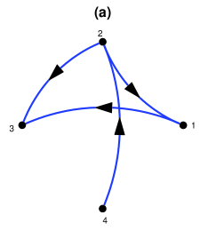
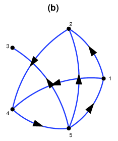
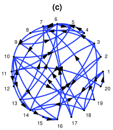
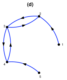
Figure 2: The graphs of the connectivity structure of the simulated systems: (a) S1, (b) S2, (c) S3, and (d) S4.

S2: A VAR(5) process on $K=4$ variables (model 1 in Winterhalder et al (2005)[49]),

$$X_{1,t} = 0.8X_{1,t-1}+0.65X_{2,t-4}+\epsilon_{1,t}$$

$$X_{2,t} = 0.6X_{2,t-1}+0.6X_{4,t-5}+\epsilon_{2,t}$$

$$X_{3,t} = 0.5X_{3,t-3}-0.6X_{1,t-1}+0.4X_{2,t-4}+\epsilon_{3,t}$$

$$X_{4,t} = 1.2X_{4,t-1}-0.7X_{4,t-2}+\epsilon_{4,t}$$

The connectivity structure of S2 is shown as graph in Figure 2b.

S3: A VAR(3) process on $K=20$ as suggested in [25]. Initially 10% of the coefficients of VAR(3) are set to one and the rest are zero and the positive coefficients are reduced iteratively until the stationarity condition is fulfilled. The autoregressive terms of lag one are set to one. The connectivity structure of S3 is shown as graph in Figure 2c.

S4: A nonlinear system, the Hénon coupled maps of $K$ variables [50, 11], where the first and last variable in the chain of $K$ variables drive their adjacent variable and the other variables drive the adjacent variable to their left and right,

$$X_{i,t}= 1.4-X_{i,t-1}^{2}+0.3X_{i,t-2},\quad\quad\mbox{for}\,\,i=1,K$$

$$X_{i,t}= 1.4-\left(0.5C(X_{i-1,t-1}+X_{i+1,t-1})+(1-C)X_{i,t-1}\right)^{2}$$

$$+0.3X_{i,t-2},\quad\quad\mbox{for}\,\,i=2,\ldots,K-1$$

Different number of variables $K$ are considered. The connectivity structure of S4 for $K=5$ is shown as graph in Figure 2d.

The systems S1, S2 and S3 are used to test the sensitivity and specificity of the methods, and the system S4 is used to assess the usefulness of the proposed restricted CGCI also when the multi-variate system is nonlinear. We make 1000 realizations for each system for different orders $p_{\mbox{\footnotesize{max}}}$ and time series length $N$.

III-B An illustrative example for VAR restriction

The performance of BTS as well as the VAR restriction methods LASSO, TDlag and BUlag on the first variable of system S1 in (III-A) in identifying the true explanatory lagged variables $X_{1,t-1}$, $X_{1,t-2}$ and $X_{5,t-1}$ is illustrated in Table I for $p_{\mbox{\footnotesize{max}}}=4$ and $N=100$.

TABLE I: Average over 1000 realizations of the coefficients estimated by the methods BTS, LASSO, TDlag and BUlag for the first variable of S1 using $p_{\mbox{\footnotesize{max}}}=4$ and $N=100$. Each cell presents the average parameter value and in parentheses the frequency of occurrence of the lagged variable in the model. The true lagged variables are highlighted in frame boxes.

	BTS	LASSO	TDlag	BUlag
$X_{1,t-1}$	0.275 (65.9%)	0.159 (51.4%)	0.433 (97.7%)	0.463 (98.9%)
$X_{1,t-2}$	-0.448 (99.9%)	-0.246 (58.2%)	-0.501 (99.8%)	-0.514 (99.9%)
$X_{1,t-3}$	-0.003 (5.1%)	-0.060 (21.6%)	-0.007 (5.8%)	0.000 (1.4%)
$X_{1,t-4}$	-0.002 (1.7%)	-0.001 (0.1%)	-0.003 (3.9%)	-0.000 (1.4%)
$X_{2,t-1}$	-0.016 (22.3%)	0.000 (0.1%)	-0.002 (5.9%)	-0.003 (3.5%)
$X_{2,t-2}$	-0.000 (1.5%)	-0.001 (0.2%)	0.002 (5.5%)	-0.002 (0.9%)
$X_{2,t-3}$	0.001 (0.9%)	0.001 (0.5%)	0.00 (7%)	-0.001 (0.4%)
$X_{2,t-4}$	-0.000 (0.4%)	-0.001 (0.7%)	-0.009 (5.8%)	-0.000 (0.1%)
$X_{3,t-1}$	0.010 (16.4%)	0.001 (1%)	0.001 (7.2%)	0.002 (3.4%)
$X_{3,t-2}$	-0.000 (3.2%)	-0.000 (0.4%)	0.002 (6.3%)	0.001 (0.6%)
$X_{3,t-3}$	0.001 (0.6%)	-0.000 (0.8%)	0.001 (4.8%)	-0.005 (0.3%)
$X_{3,t-4}$	-0.001 (0.2%)	-0.000 (0.6%)	-0.001 (6.5%)	-0.000 (0.1%)
$X_{4,t-1}$	-0.009 (7.5%)	-0.000 (0.1%)	0.006 (5.4%)	0.004 (5.2%)
$X_{4,t-2}$	0.001 (1%)	-0.000 (0.1%)	-0.004 (6.2%)	-0.006 (2.4 %)
$X_{4,t-3}$	-0.000 (0.3%)	-0.000 (0.4%)	-0.005 (5.8%)	0.000 (2.5%)
$X_{4,t-4}$	-0.000 (0.1%)	-0.000 (0.2%)	-0.001 (5.6%)	0.001 (0.7%)
$X_{5,t-1}$	0.424 (99.7%)	0.379 (82.8%)	0.174 (39%)	0.114 (25.7%)
$X_{5,t-2}$	0.012 (8.7%)	0.011 (3.7%)	0.014 (7.2%)	0.083 (3.6%)
$X_{5,t-3}$	-0.001 (2.9%)	-0.000 (0.1%)	-0.005 (6.3%)	-0.004 (0.6%)
$X_{5,t-4}$	-0.001 (0.7%)	-0.007 (2.7%)	-0.003 (6.3%)	-0.000 (0.3%)

All restriction methods reduce the full representation of 20 lagged variables to few lagged variables, most often being only the true three lagged variables, so that the average values of the coefficients from 1000 Monte Carlo realizations are close to zero for all but the three true lagged variables. The false detection is very low for TDlag and BUlag at about the 5% significance level (highest at 7.2% and 5.2%, respectively), and higher for LASSO but at only one lagged variable (21.6% for $X_{1,t-3}$), and for BTS at two lagged variables (22.3% and 16.4% for $X_{2,t-1}$ and $X_{3,t-1}$). On the other hand, BTS includes the true lagged variables most often in the DR model, $X_{1,t-1}$ at 65.9% of the runs and $X_{1,t-2}$ and $X_{5,t-1}$ almost always, whereas the frequencies for LASSO are respectively 51.4%, 58.2% and 82.8%, and for TDlag and BUlag the first two are almost always included while $X_{5,t-1}$ is included at a low rate of 39% and 25.7%, respectively. These results suggest that CGCI on the basis of BTS would always detect the true driving effect $X_{5}\rightarrow X_{1}$ (highest sensitivity) but also the false driving effects $X_{2}\rightarrow X_{1}$ and $X_{3}\rightarrow X_{1}$ at a small but significant percentage of cases (lower specificity), whereas the other three methods would have high specificity (infrequently detecting the driving effects from $X_{2}$, $X_{3}$ and $X_{4}$ to $X_{1}$) but lower sensitivity as the true lagged variable $X_{5,t-1}$ would not always enter the model.

III-C System 1

The example above is for the dynamic regression of variable $X_{1}$ of S1, and in the following we present the Granger causality effects for all variables of S1. The true Granger causality effects between any variables of S1 are defined by the lagged variables being present in the dynamic regression of each of the five variables of S1 in (III-A), being $X_{1}\rightarrow X_{2}$, $X_{1}\rightarrow X_{4}$, $X_{2}\rightarrow X_{4}$, $X_{4}\rightarrow X_{5}$, $X_{5}\rightarrow X_{1}$, $X_{5}\rightarrow X_{2}$ and $X_{5}\rightarrow X_{3}$.

The rate of detection of the true Granger causality effects varies with the method and the order, as shown in Figure 3 for $p_{\mbox{\footnotesize{max}}}=5$ and $p_{\mbox{\footnotesize{max}}}=10$.

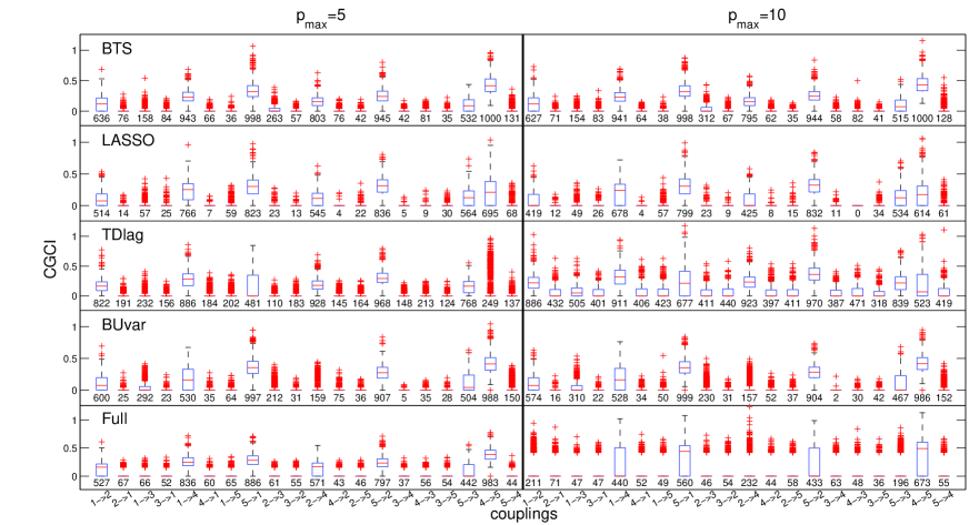
Figure 3: Boxplots of CGCI for all variable pairs of S1 and $N=100$, from 1000 realizations,for $p_{\mbox{\footnotesize{max}}}=5$ at the left panels and $p_{\mbox{\footnotesize{max}}}=10$ at the right panels, and for the methods BTS, LASSO, TDlag, BUvar and Full going from top to bottom panels. At each panel the number of statistically significant CGCI is displayed below each boxplot. The true causality effects are: $X_{1}\rightarrow X_{2}$, $X_{1}\rightarrow X_{4}$, $X_{5}\rightarrow X_{1}$, $X_{2}\rightarrow X_{4}$, $X_{5}\rightarrow X_{2}$, $X_{5}\rightarrow X_{3}$ and $X_{4}\rightarrow X_{5}$.

The boxplots display the distribution of CGCI over the 1000 realizations for each ordered pair of variables and the number below each boxplot is the number of times CGCI was found statistically significant at $\alpha=0.05$ using the FDR correction.

For $p_{\mbox{\footnotesize{max}}}=5$ being only one larger than the correct order, LASSO, BTS and Full identify the seven true causality effects at large percentages of the 1000 realizations, with BTS scoring highest. The largest difference is observed for $X_{2}\rightarrow X_{4}$ and the detection percentage of BTS is 80.3% to be compared with 54.5% for LASSO and 57.1% for Full. However, BTS detects at a significant rate also false causality effects (e.g. detection percentage 26.3% for $X_{2}\rightarrow X_{3}$ as shown in Figure 3), whereas LASSO and Full do not exceed the significance level of 5%. TDlag fails to detect the coupling $X_{4}\rightarrow X_{5}$ (detection percentage 24.9%) and BUvar the coupling $X_{1}\rightarrow X_{3}$ (detection percentage 29.2%), whereas they both give false causality effects at a significantly high rate. These results suggest that the bottom-up and top-down strategies are influenced by the order in which the variables enter or leave the DR model, respectively.

When $p_{\mbox{\footnotesize{max}}}$ increases to 10, BTS and BUvar are the most stable giving the same results, whereas LASSO tends to detect Granger causality effects at a somewhat smaller rate, Full does the same at a larger extent so that three true couplings are detected at a rate smaller than 25%, and TDlag increases the detection rate of all couplings.

For each realization we calculate the measures sensitivity, specificity, MCC, F-measure and Hamming distance on the basis of the significance of CGCI for all pairs of variables of S1. We also statistically compare the measures for mBTS and each of the other methods. In Table II, the results on these performance indices and the restriction methods, as well as Full, are shown for $p_{\mbox{\footnotesize{max}}}=5$ and $p_{\mbox{\footnotesize{max}}}=10$ and $N=100$.

TABLE II: Sensitivity (SENS), specificity (SPEC), MCC, F-measure (FM) and Hamming distance (HD) (average value and standard deviation in parentheses) of the causality methods for S1, $p_{\mbox{\footnotesize{max}}}=5,10$ and $N$=100. The highest score at each performance index and $p_{\mbox{\footnotesize{max}}}$ is highlighted.The statistical significance for the mean difference of a measure on BTS and another method is denoted with a superscript symbol ’⁺’ when the difference is positive and ’^-’ when it is negative.

	$p$	BTS	LASSO	BUlag	BUvar	TDlag	TDvar	Full
SENS	5	0.823	0.673+	0.421+	0.656+	0.708+	0.937-	0.556+
(SD)		(0.126)	(0.171)	(0.167)	(0.139)	(0.145)	(0.087)	(0.184)
	10	0.819	0.612+	0.414+	0.650+	0.794+	0.953-	0.156+
		(0.125)	(0.178)	(0.167)	(0.138)	(0.36)	(0.080)	(0.143)
SPEC	5	0.935	0.977-	0.950-	0.938	0.880+	0.762+	0.984-
(SD)		(0.073)	(0.041)	(0.061)	(0.064)	(0.103)	(0.143)	(0.037)
	10	0.934	0.979-	0.954-	0.935	0.651+	0.401+	0.990-
		(0.071)	(0.040)	(0.058)	(0.066)	(0.167)	(0.168)	(0.033)
MCC	5	0.775	0.717+	0.461+	0.643+	0.611+	0.681+	0.637+
(SD)		(0.155)	(0.154)	(0.201)	(0.159)	(0.177)	(0.158)	(0.154)
	10	0.746	0.672+	0.463+	0.634+	0.439+	0.379+	0.248+
		(0.166)	(0.161)	(0.191)	(0.163)	(0.184)	(0.162)	(0.197)
FM	5	0.846	0.773+	0.542+	0.736+	0.732+	0.796+	0.683+
(SD)		(0.104)	(0.135)	(0.173)	(0.116)	(0.118)	(0.096)	(0.160)
	10	0.843	0.727+	0.537+	0.730+	0.655+	0.627+	0.240+
		(0.105)	(0.151)	(0.0.171)	(0.119)	(0.100)	(0.073)	(0.199)
HD	5	2.084	2.587+	4.707+	3.217+	3.608+	3.528+	3.321+
(SD)		(1.428)	(1.342)	(1.509)	(1.373)	(1.650)	(1.920)	(1.312)
	10	2.123	2.995+	4.702+	3.295+	5.978+	8.120+	6.032+
		(1.430)	(1.385)	(1.437)	(1.411)	(2.148)	(2.205)	0.972

BTS has high sensitivity and specificity, though it does not score highest in both. The highest sensitivity score is obtained by TDvar at 0.937 for $p_{\mbox{\footnotesize{max}}}=5$ and 0.953 for $p_{\mbox{\footnotesize{max}}}=10$, both being statistically significantly higher than for BTS, but TDvar scores lowest of all methods in specificity. Similarly, Full scores highest in specificity at 0.984 for $p_{\mbox{\footnotesize{max}}}=5$ and 0.990 for $p_{\mbox{\footnotesize{max}}}=10$, both significantly higher than for BTS, but has the lowest sensitivity, which for $p_{\mbox{\footnotesize{max}}}=10$ is remarkably low at 0.156. The latter indicates the inappropriateness of the standard Granger causality estimated by the full VAR model when the order is large. The high sensitivity and specificity of BTS makes it score highest in all three performance indices combining sensitivity and specificity, and the difference is statistically significant for all methods and for all three indices. Second best in MCC, FM and Hamming distance is LASSO giving somewhat higher specificity than BTS but much lower sensitivity (for FM TDvar scores slightly higher than LASSO when $p_{\mbox{\footnotesize{max}}}=5$ and BUvar when $p_{\mbox{\footnotesize{max}}}=10$). All the methods restricting the VAR model are robust to the increase of $p_{\mbox{\footnotesize{max}}}$ and give approximately the same performance index values, while the performance of Full drops drastically, e.g. the number of false positives and negatives counted by the Hamming distance are doubled (from about 3 to 6) going from $p_{\mbox{\footnotesize{max}}}=5$ to $p_{\mbox{\footnotesize{max}}}=10$. The bottom-up strategies BUlag and BUvar have as high specificity as BTS but much lower sensitivity, especially BUlag. Thus for this system, the time-lag supervised bottom-up search in BTS manages to spot the correct lagged variables better than an arbitrary bottom-up search of BUlag and BUvar. The results for all methods vary across realizations but at about the same amount, which is larger for the sensitivity than for the specificity, as indicated by the standard deviation (SD) values. Full and LASSO tend to have the largest SD of sensitivity and smallest SD of specificity, which amounts the same SD of MCC as for BTS but larger SD of the FM than for BTS. We note that the SD is moderately large with respect to the average values but allows for the mean differences to be statistically significant.

The results in Table II are obtained using the significance test for CGCI corrected with FDR. If no correction for multiple testing is applied the sensitivity increases at the cost of lower specificity and the overall performance measured by MCC, F-measure and Hamming distance is somewhat lower. If no significance testing is performed, and the existence of coupling is determined simply by a zero or positive CGCI (this is not applied to Full), the sensitivity is further increased but the specificity is disproportionately decreased, giving smaller overall performance indices. For example, for BTS and $p_{\mbox{\footnotesize{max}}}=5$, the sensitivity increases from 0.823 to 0.867 but the specificity drops from 0.935 to 0.821, so that MCC drops from 0.775 to 0.674. The same feature is observed for all but LASSO methods restricting VAR, so that the superiority of BTS is maintained also when significance testing is not performed, and it remains superior to Full, which is always applied with the significance test. It is noted that LASSO cannot be included in this comparison as it contains a significance test for the model coefficients (the covariance test, see Sec. II-D), and thus it gives about the same results with and without the significance test for CGCI.

III-D System 2

In Table III, the average sensitivity, specificity and MCC from 1000 realizations are shown for system S2 using as maximum order the true VAR order ($p_{\mbox{\footnotesize{max}}}=5$) and different time series lengths $N=50,100,1000$.

TABLE III: Average sensitivity (SENS), specificity (SPEC) and MCC of the causality methods for system S2, $p_{\mbox{\footnotesize{max}}}=5$ and $N=50,100,1000$. The highest score at each performance index and $N$ is highlighted. The statistical significance for the mean difference of a measure on BTS and another method is denoted with a superscript symbol ’⁺’ when the difference is positive and ’^-’ when it is negative.

	$N$	BTS	LASSO	BUlag	BUvar	TDlag	TDvar	Full
SENS	50	0.916	0.774+	0.857+	0.848+	0.964-	0.985-	0.727+
	100	0.996	0.919+	0.939+	0.935+	0.996	1.0-	0.993
	1000	1.0	0.999	1.0	1.0	1.0	1.0	1.0
SPEC	50	0.947	0.976 -	0.958-	0.962-	0.848+	0.747+	0.976-
	100	0.967	0.978-	0.977-	0.974-	0.921+	0.826+	0.973
	1000	0.987	0.981+	0.993-	0.992-	0.982+	0.865+	0.976+
MCC	50	0.868	0.799+	0.838+	0.836+	0.796 +	0.713+	0.762+
	100	0.955	0.910+	0.924+	0.918+	0.901+	0.803+	0.961
	1000	0.983	0.975+	0.991-	0.989-	0.977+	0.843+	0.969+

For $N=50$ and $100$ the highest sensitivity score is obtained by TDvar, at 0.985 and 1.0 respectively, but this method scores lowest in specificity. For $N=1000$, all methods detect the true couplings and score 1.0 in sensitivity (almost 1.0 for LASSO). For $N=50$, the highest specificity score is obtained by LASSO and Full but both have the lowest score in sensitivity. When $N$ increases, the specificity, as well as the sensitivity and MCC, approaches 1.0 for all but TDvar methods. BTS method may not rank first in sensitivity and specificity but consistently presents high values for all time series lengths, so that it scores highest in MCC for $N=50$ and follows closely with the highest MCC for larger $N$. It is also noted that BTS scores higher in MCC than LASSO for all time series lengths. All the mean differences in the indices between BTS and any of the other measures are found statistically significant (see the plus and minus superscripts in Table III).

III-E System 3

System 3 is VAR on 20 variables and order three and has 10% non-zero coefficients of a total of 1200 coefficients, giving respectively 10% true couplings of a total of 380 possible ordered couplings. Considering the DR model for each of the 20 variables, the total number of coefficients is 60 and thus Full cannot provide stable solution when $N$ is as small as 100, being unable to identify Granger causality effects and giving therefore a very small sensitivity value, 0.002, as shown in Table IV.

TABLE IV: Average sensitivity (SENS), specificity (SPEC) and MCC of the causality methods for S3, and combinations of $p_{\mbox{\footnotesize{max}}}=4,5$ and $N=100,200,500$.The statistical significance for the mean difference of a measure on BTS and another method is denoted with a superscript symbol ’⁺’ when the difference is positive and ’^-’ when it is negative.

	$p$	$N$	BTS	LASSO	BUlag	BUvar	TDlag	TDvar	Full
SENS	4	100	0.238	0.091 +	0.233	0.228+	0.624-	0.690-	0.002+
	4	200	0.506	0.258+	0.576-	0.583-	0.718-	0.793-	0.064+
	5	500	0.959	0.791+	0.949+	0.964-	0.978-	0.993-	0.775+
SPEC	4	100	0.989	0.998-	0.990	0.991	0.637+	0.524+	0.999 -
	4	200	0.996	0.999-	0.992+	0.992+	0.945+	0.834+	0.999
	5	500	0.992	0.997-	0.994+	0.993+	0.966+	0.882+	0.995-
MCC	4	100	0.373	0.248+	0.373	0.376-	0.164+	0.131+	0.004+
	4	200	0.664	0.470+	0.693-	0.695-	0.616+	0.457+	0.198+
	5	500	0.941	0.788+	0.942	0.948-	0.942	0.659+	0.845+

Neither for $N=200$, Full identifies the true Granger causality effects (sensitivity at 0.064), and it achieves this when $N=500$, scoring still lowest of all methods. The highest score in sensitivity is obtained by TDvar for all $N$, being significantly higher than for BTS, but again it scores lowest in specificity for all $N$. Highest in specificity is again Full competing with LASSO for the first place, but all but the top-down strategies score almost equally high, still being both significantly higher than for BTS. LASSO scores much lower in sensitivity so that overall it performs purely in this high-dimensional system. The best performance, as quantified by MCC, is again exhibited by the bottom-up strategies, with BTS scoring slightly below the largest MCC obtained by BUvar, but this difference is found statistically significant. The other methods (LASSO, TDlag and TDvar, Full) do much worse and do not approach as $N$ increases the level of bottom-up strategies. For example for $N=500$, the bottom-up strategies give MCC about 0.94, whereas the other methods score up to 0.85.

III-F System 4

Many real world problems may involve nonlinear causality relationships and it is therefore of interest to assess at what extent the linear Granger causality methods can estimate correctly nonlinear causal effects. Certainly, for a comprehensive assessment by means of a simulation study one should include systems having different forms of nonlinear relationships, but here we restrict ourselves to system S4, a known testbed for nonlinear Granger causality methods. We consider in the comparison two nonlinear causality methods based on information theory, the partial transfer entropy (PTE) computed on embedding vectors from each variable corresponding to CGCI on the full VAR representation [35, 36], and the partial mutual information on mixed embedding (PMIME) computed on restricted mixed embedding vectors from all variables corresponding to CGCI on the restricted VAR representation [51, 11]. PTE is the extension of the widely used bivariate transfer entropy (TE) [10], taking into account the presence of the other observed variables. PMIME first searches for the most relevant lagged variables to the response $X_{j}$ using the conditional mutual information. Then similarly to the definition of PTE, PMIME quantifies the information of the lagged variables of the driving variable $X_{i}$ to the response variable $X_{j}$. For the entropy estimation in both PTE and PMIME the estimate of $k$-nearest neighbors is used [52]. Figure 4 shows the value of MCC for different number of variables $K$ and for time series lengths $N=512,1024$, for the latter reporting also results for PMIME and PTE (obtained from 100 realizations as opposed to 1000 realizations used for the linear methods).

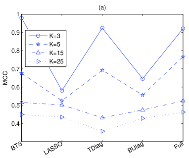
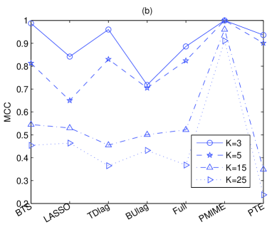
Figure 4: MCC vs method as given in the x-axis for S5 (coupled Hénon maps), $p_{\mbox{\footnotesize{max}}}=5$ and number of variables $K$ as given in the legend. (a) $N=512$, (b) $N=1024$, including the nonlinear methods PMIME and PTE.

We observe that among the linear methods, for small $K$ BTS is the best followed by TDlag and LASSO is the worst, whereas for larger $K$ BTS is again the best followed closely by LASSO and the worst is TDlag. BUlag performs similarly to LASSO and Full similarly to BTS scoring highest for $N=512$ and $K=5$. Full still scores high for large $K$ and all linear methods have reduced specificity as $K$ increases scoring low in MCC. This is to be contrasted to PMIME for $N=1024$ obtaining MCC$>$0.9 even for $K=25$, whereas PTE fails when $K$ gets large ($K=15,25$), because it does not apply any restriction to the lagged variables.

Dealing with systems of many variables, high order and long time series, the computation cost may be an issue, and it is known that a main shortcoming of LASSO is the computation time. It is not easy to give exact figures for the computational complexity, as it depends on the sparsity of the matrix of the lagged variables of the true system. The computational complexity can be measured in terms of the tested models, and for BTS it is a multiple of the number $K$ of variables in the model, comparable (slightly larger) to that for the bottom-up and top-down strategies. To the contrary, the computational time of LASSO is much larger. As mentioned above, LASSO is computed in two parts: the different models derived for increasing tuning parameter $s$ (’lars’ function) and the selection of the final model using the covariance test (’covTest’ function). We counted the computation times for the two parts of LASSO in the simulations for different systems, time series lengths and orders and we concluded that the second part is the most time consuming. For example, for one realization of the S1 system ($N=100$, $p_{\mbox{\footnotesize{max}}}=10$, $K=5$) and for all $K$ variables, LASSO was completed in 2.81 s (first part: 0.77 s, second part: 2.04 s) while BTS in 0.10 s . Also, for one realization of the S3 system ($N=500$, $p_{\mbox{\footnotesize{max}}}=5$, $K=20$), LASSO was completed in 83.46 s (first part: 1.22 s, second part: 82.236 s) while BTS in 2.59 s. Overall, in the simulation study LASSO was found to be about 20 times slower than BTS, which in turn is more than 5 times slower than the top-down and bottom-up strategies, the latter giving about the same computation times.

IV Application to real data

In this application we assess whether the VAR restriction allows for a better quantification of the Granger causality effects between brain areas, known also as effective connectivity [53]. The dataset is a scalp multi-channel electroencephalographic (EEG) recording of a patient with epilepsy containing 8 episodes of epileptiform discharge (ED), i.e. a small electrographic seizure of very small duration. The recording was done at the Laboratory of Clinical Neurophysiology, Medical School, Aristotle University of Thessaloniki. The EEG data were initially sampled at 1450 Hz and downsampled to 200 Hz, band-pass filtered at [0.3,70] Hz (FIR filter of order 500), initially referenced to the right mastoid and re-referenced to infinity. Channels with artifacts were removed resulting in 44 artifact-free channels. For each of the 8 episodes, the ED is terminated by the administration of transcranial magnetic stimulation (TMS) (a block of 5 TMS at 5 Hz frequency). For details on the experimental setup see [54, 55]. For all episodes, we considered a data window of about 23 sec including a part before the ED, the ED and a part after the ED. Each data window was split to overlapping sliding windows of duration 2 sec and sliding step 1 sec. We consider three states for each episode, the preED state regarding the first 9 windows before the ED start, the ED state covering the ED (3-5 windows, depending on the episode), and the postED state regarding the time after the end. The interest is in discriminating the three states on the basis of the connectivity (causality) structure of the EEG channels.

The brain (effective) connectivity structure can be better seen in a network form, where the nodes of the network are the EEG channels and the weighted connections of the network are given by the corresponding CGCI values. Certainly, we cannot anticipate the detection of specific causality effects between any channels, but we expect that the overall connectivity is different during ED than before and after ED. The brain connectivity obtained by CGCI can be quantified using network measures, and here we summarize the connectivity of each channel by the out-strength of the node at each sliding window, $s_{i}=\frac{1}{K-1}\sum_{j=1}^{K}\mbox{CGCI}_{i\rightarrow j}$, the total driving effect of channel $i$ to all other $K$ channels, and thereafter we compute the average strength over all nodes, $S=\frac{1}{K}\sum_{i=1}^{K}s_{i}$.

CGCI derived by BTS exhibits a clear increase in connectivity during ED, whereas there are few causal effects at the preED and postED state. An example of the $s_{i}$ across all time windows of one episode is shown in Figure 5a.

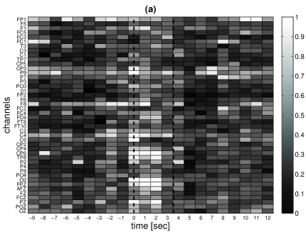
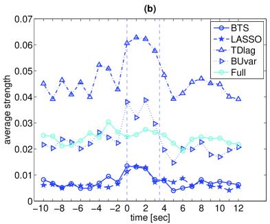
Figure 5: (a) Color map of node (EEG channel) strength with BTS method in successive windows across one ED episode for $p_{\mbox{\footnotesize{max}}}=3$ and $N=400$. (b) The average strength for the VAR restriction methods and Full, as shown in the legend, for successive sliding windows and the same episode as in (a). The dashed lines indicate the start and end of ED and the time is given with reference to the ED start.

The increased connectivity at the ED state is observed mostly at the frontal and central channels (channel names starting with “F” or “C” at the lower part of Figure 5a), whereas the occipital channels (names starting with “O”) exhibit almost no connectivity during ED and some low-level connectivity during preED and postED.

The $S$ as a function of the time window for the same episode is shown in Figure 5b for the VAR restriction methods BTS, LASSO, TDlag, BUvar, as well as Full. It is clearly shown that $S$ increases during ED for the VAR restriction methods but not for Full, for which $S$ fluctuates regardless of the state. We also tested larger $p_{\mbox{\footnotesize{max}}}$ values, but the difference between preED, ED and postED was depicted better for $p_{\mbox{\footnotesize{max}}}=3$. The differences in the range of strength across different methods, as shown in Figure 5b, is due to the different number of variables (EEG channels) selected by the methods in the dynamic regression model. For example, in the DR of $X_{40}$, 12 variables are found by BTS, 7 by LASSO, 27 by TDlag and 16 by BUvar. As the number of variables increases in the DR so does the number of causal effects and subsequently the connections in the network. Despite this difference, all restriction methods reveal well the difference between the states.

To assess the statistical significance of the change of connectivity from the preED state to the ED state and back to the postED states, we applied paired samples student test for each of the pair differences preED-ED, postED-ED and preED-postED state, where the sample for each state contains 8 observations, and each observation is the average of the network strength $S$ over all windows for the corresponding state in an episode. In Figure 6, the boxplots for the three pair differences in $S$ derived by BTS and Full are presented.

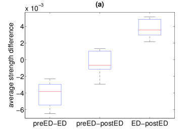
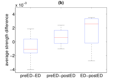
Figure 6: Boxplots for the average strength differences of preED-ED, preED-postED and ED-posteED from 8 episodes:(a) BTS and $p_{\mbox{\footnotesize{max}}}=3$,(b) Full and $p_{\mbox{\footnotesize{max}}}=3$.

For BTS, the mean differences preED-ED and ED-postED are found statistically significant ($p=0.00012$ and $p=0.00003$, respectively) and the same was obtained by the Wilcoxon sign rank test, whereas the difference preED-postED is not found statistically significant. The same significant differences could be established also with the other VAR restricting methods but TDlag. On the other hand, for Full statistically significant difference could not be established for any states. This finding indicates the necessity of using VAR restriction methods when the linear Granger causality index has to be computed on a large number of EEG channels.

V Discussion

We introduce a new approach in forming the classical conditional Granger causality index (CGCI) for the estimation of the Granger causality in time series of many variables, i.e. instead of deriving CGCI on the full vector autoregressive (VAR) representation, we suggest a restriction of VAR using the method of backward-in-time selection (BTS). We call this approach BTS-CGCI. BTS is a bottom-up strategy and it builds up the dynamic regression model progressively searching first for lagged variables temporally closer to the response variable. This supervised search is designed exactly for time series problems, unlike other methods, such as LASSO, being developed for regression problems. We propose a modified BTS, which results in specific lagged variables instead of all the lagged variables up to a selected order. For the inclusion of a lagged variable in the model, the Bayesian information criterion (BIC) is utilized. The same criterion is used also in the implementation of the bottom-up and top-down strategies, to which BTS is compared. It is noted that the criterion of final prediction error (FPE) was used in the simulations, and gave qualitatively similar results.

The use of BTS allows for a convenient deduction of lack of Granger causality from CGCI. If the dynamic regression model obtained by BTS does not contain any components of the driving variable then CGCI is set to zero and there is no Granger causality effect. Otherwise, this model is considered as the unrestricted model (containing the driving variable components) and the restricted model is derived by omitting the components of the driving variable. Then CGCI is computed on the basis of these two models, as in the standard definition of CGCI. Furthermore, significance test on CGCI can be performed as for the CGCI with the full VAR (correcting also for multiple testing). However, for applications where parametric significance testing cannot be trusted due to deviation from normality, a positive CGCI derived from BTS can be considered as significant. The simulation study showed that this simpler approach gains better sensitivity in detecting causal effects than when using the significance test. On the other hand, it tends to give more false positives so that overall the implementation with the significance testing should be preferred when it is applicable.

BTS was compared to other VAR restriction methods, i.e. bottom-up and top-down strategies and LASSO, in their ability to identify the correct causal relationships. The simulation results in the cases of three VAR processes and a nonlinear coupled dynamical system showed that BTS had the overall best performance scoring consistently high in the performance indices of sensitivity, specificity, Matthews correlation coefficient (MCC), F-measure (FM) and Hamming distance. The other methods had varying performance, and in particular LASSO scored generally low. Differences among the methods were particularly revealed at small time series lengths $N$, whereas for larger $N$ all methods tended to converge in estimating the correct causal effects. However, this was not true for the full VAR representation (the standard approach) whenever the VAR order was large. For small $N$, LASSO and the full VAR tended to have the highest specificity but relatively low sensitivity, whereas the top-down strategy tended to have the highest sensitivity but also the lowest specificity. On the other hand, BTS scored always high in both sensitivity and specificity, resulting in the highest or close to the highest score in MCC, F-measure and Hamming distance in all settings. We attribute the good performance of CGCI with BTS to the design of BTS that unlike the other methods it was developed for time series (not regression in general) making use of the time order of the lagged variables.

Our simulation study confirmed the computational shortcoming of LASSO of being much slower than all other methods. The top-down strategy requires the estimation of the full model in the initial step, thus it bears the same shortcoming as the full VAR for many variables and short time series. On the other hand, the bottom-up strategy and BTS start from few (actually none) degrees of freedom adding one lagged variable at a time, and therefore they are both computationally and operationally effective for short time series even when the number of time series is very large. LASSO can also be used in this setting but not in conjunction with the covariance test that gives the significant lagged variable terms. Thus BTS can be applied even in settings where the number of variables exceeds the time series length, as for example in gene microarrays experiments.

We confirmed the significance of BTS along with the other VAR restriction methods in an application of epileptiform discharge observed in electroencephalograms. We could clearly detect the change of brain connectivity during the epileptiform discharge with the VAR restricted methods that could not be revealed by the full VAR.

In some applications, and particularly in econometrics, the Granger causality has to be estimated in non-stationary time series. If the time series are also co-integrated, the model of choice is the vector error correction model (VECM) that contains a full VAR model for the first differenced variables [56]. The dimension reduction, and mBTS in particular, can be extended to restrict the VAR part in VECM, but the implementation is not straightforward and is left for future work. If the time series are not co-integrated then the non-stationarity for each time series separately is first removed, e.g. taking first differences, and the dimension reduction method can then be applied to the stationary time series in a straightforward manner.

In summary, the main aspects of the proposed approach are:

• The dimension reduction methods provide overall better estimation of Granger causality than the standard full VAR approach.

• The recently developed dimension reduction method of backward-in-time selection (BTS) has been modified (mBTS), so as to give the exact lagged variables being the most explanatory to the response variable.

• The proposed mBTS method uses a time ordered supervised sequential selection of the lagged variables, tailored for time series, as opposed to other methods that do not take into account the time order, being developed for regression problems (bottom-up, top-down, LASSO).

• The simulation study showed that mBTS estimates overall better the Granger causality than other tested dimension reduction methods (bottom-up, top-down, LASSO) and the standard VAR approach.

• The proposed mBTS method is particularly useful for high dimensional time series of short length, as demonstrated in the application to epileptic EEG.

The Matlab codes for mBTS and CGCI are given in the second author’s homepage, currently being http://users.auth.gr/dkugiu/.

VI Acknowledgments

The work is supported by the Greek General Secretariat for Research and Technology (Aristeia II, No 4822). The authors want to thank Vasilios Kimiskidis, at Aristotle University of Thessaloniki, for providing the EEG data, and Ioannis Rekanos, at Aristotle University of Thessaloniki for valuable comments and discussions.

References

- [1] H. Lütkepohl, New Introduction to Multiple Time Series Analysis. Berlin Heidelberg: Springer-Verlag, 2005.
- [2] G. Kirchgässner and J. Wolters, Introduction to Modern Time Series Analysis. Berlin, Heidelberg: Springer-Verlag, 2007.
- [3] K. Hoover, Causality in economics and econometrics, The New Palgrave Dictionary of Economics, 2nd ed. Palgrave Macmillan, 2008.
- [4] L. Faes, R. G. Andrzejak, M. Ding, and D. Kugiumtzis, “Editorial: Methodological advances in brain connectivity,” Computational and Mathematical Methods in Medicine, vol. 2012, p. 492902, 2012.
- [5] J. Granger, “Investigating causal relations by econometric models and cross-spectral methods,” Acta Physica Polonica B, vol. 37, pp. 424–438, 1969.
- [6] J. F. Geweke, “Measures of conditional linear dependence and feedback between time series,” Journal of the American Statistical Association, vol. 79, no. 388, pp. 907–915, 1984.
- [7] S. Guo, A. K. Seth, K. Kendrick, C. Zhou, and J. Feng, “Partial Granger causality – eliminating exogenous inputs and latent variables,” Journal of Neuroscience Methods, vol. 172, pp. 79–93, 2008.
- [8] L. Baccala and K. Sameshima, “Partial directed coherence: a new concept in neural structure determination,” Biological Cybernetics, vol. 84, no. 6, pp. 463 – 474, 2001.
- [9] A. Korzeniewska, M. Manczak, M.and Kaminski, K. Blinowska, and S. Kasicki, “Determination of information flow direction between brain structures by a modified directed transfer function method (ddtf),” Journal of Neuroscience Methods, vol. 125, pp. 195–207, 2003.
- [10] T. Schreiber, “Measuring information transfer,” Physical Review Letters, vol. 85, no. 2, pp. 461–464, 2000.
- [11] D. Kugiumtzis, “Direct-coupling information measure from nonuniform embedding,” Physical Review E, vol. 87, p. 062918, 2013.
- [12] J. Arnhold, P. Grassberger, K. Lehnertz, and C. E. Elger, “A robust method for detecting interdependences: Application to intracranially recorded EEG,” Physica D, vol. 134, pp. 419–430, 1999.
- [13] D. Chicharro and R. Andrzejak, “Reliable detection of directional couplings using rank statistics,” Physical Review E, vol. 80, p. 026217, 2009.
- [14] D. Smirnov and B. Bezruchko, “Estimation of interaction strength and direction from short and noisy time series,” Physical Review E, vol. 68, no. 4, p. 046209, 2003.
- [15] T. Kreuz, F. Mormann, R. Andrzejak, A. Kraskov, K. Lehnertz, and P. Grassberger, “Measuring synchronization in coupled model systems: A comparison of different approaches,” Physica D, vol. 225, no. 1, pp. 29–42, 2007.
- [16] A. Papana, C. Kyrtsou, D. Kugiumtzis, and C. Diks, “Simulation study of direct causality measures in multivariate time series,” Entropy, vol. 15, no. 7, pp. 2635–2661, 2013.
- [17] A. Miller, Subset Selection in Regression, 2nd ed. Chapman & Hall/CRC, 2002.
- [18] T. Hastie, R. Tibshirani, and J. Friedman, The Elements of Statistical Learning, Data Mining, Inference, and Prediction, 2nd ed. New York, NY: Springer-Verlag, 2009.
- [19] J. H. Stock and M. W. Watson, “Chapter 10 forecasting with many predictors,” in Handbook of Economic Forecasting, ser. Handbook of Economics, G. Elliott, C. W. J. Granger, and A. Timmermann, Eds. Elsevier, 2006, vol. 1, pp. 515 – 554.
- [20] I. Vlachos and D. Kugiumtzis, “Backward-in-time selection of the order of dynamic regression prediction model,” Journal of Forecasting, vol. 32, pp. 685–701, 2013.
- [21] A. Arnold, Y. Liu, and N. Abe, “Temporal causal modeling with graphical Granger methods,” in Proceedings of the ACM SIGKDD International Conference on Knowledge Discovery and Data Mining, 2007, pp. 66–75.
- [22] A. C. Lozano, N. Abe, Y. Liu, and S. Rosset, “Grouped graphical Granger modeling methods for temporal causal modeling,” in Proceedings of the ACM SIGKDD International Conference on Knowledge Discovery and Data Mining, 2009, pp. 577–585.
- [23] A. Shojaie and G. Michailidis, “Discovering graphical Granger causality using the truncating lasso penalty,” Bioinformatics, vol. 26, no. 18, pp. i517–i523, 2010.
- [24] Y. He, Y. She, and D. Wu, “Stationary-sparse causality network learning,” Journal of Machine Learning Research, vol. 14, pp. 3073–3104, 2013.
- [25] S. Basu and G. Michailidis, “Regularized estimation in sparse high-dimensional time series models,” Annals of Statistics, vol. 43, no. 4, pp. 1535–1567, 2015.
- [26] N.-J. Hsu, H.-L. Hung, and Y.-M. Chang, “Subset selection for vector autoregressive processes using Lasso,” Computational Statistics & Data Analysis, vol. 52, no. 7, pp. 3645–3657, 2008.
- [27] Y. Ren and X. Zhang, “Subset selection for vector autoregressive processes via adaptive Lasso,” Statistics & Probability Letters, vol. 80, no. 23-24, pp. 1705–1712, 2010.
- [28] ——, “Model selection for vector autoregressive processes via adaptive Lasso,” Communications in Statistics - Theory and Methods, vol. 42, no. 13, pp. 2423–2436, 2013.
- [29] D. Gefang, “Bayesian doubly adaptive elastic-net Lasso for VAR shrinkage,” International Journal of Forecasting, vol. 30, no. 1, pp. 1–11, 2014.
- [30] S. Haufe, R. Tomioka, G. Nolte, K.-R. Müller, and M. Kawanabe, “Modeling sparse connectivity between underlying brain sources for EEG/MEG,” IEEE Transactions on Biomedical Engineering, vol. 57, no. 8, pp. 1954–1963, 2010.
- [31] W. Tang, S. L. Bressler, C. M. Sylvester, G. L. Shulman, and M. Corbetta, “Measuring Granger causality between cortical regions from voxelwise fMRI BOLD signals with LASSO,” PLoS Computational Biology, vol. 8, no. 5, 2012.
- [32] A. Pongrattanakul, P. Lertkultanon, and J. Songsiri, “Sparse system identification for discovering brain connectivity from fMRI time series,” in Proceedings of the SICE Annual Conference, 2013, pp. 949–954.
- [33] A. Fujita, J. Sato, R. Garay-Malpartida, H.and Yamaguchi, S. Miyano, M. Sogayar, and C. Ferreira, “Modeling gene expression regulatory networks with sparse autoregressive model,” BioMed Central, vol. 1:39, 2007.
- [34] A. Shojaie, S. Basu, and G. Michailidis, “Adaptive thresholding for reconstructing regulatory networks from time-course gene expression data,” Statistics in Biosciences, vol. 4, no. 1, pp. 66–83, 2012.
- [35] V. A. Vakorin, O. A. Krakovska, and A. R. McIntosh, “Confounding effects of indirect connections on causality estimation,” Journal of Neuroscience Methods, vol. 184, pp. 152–160, 2009.
- [36] A. Papana, D. Kugiumtzis, and P. G. Larsson, “Detection of direct causal effects and application in the analysis of electroencephalograms from patients with epilepsy,” International Journal of Bifurcation and Chaos, vol. 22, no. 9, p. 1250222, 2012.
- [37] A. Pankratz, Forecasting with Dynamic Regression Models. New York: Wiley, 1991.
- [38] P. T. Brandt and J. T. Williams, Multiple Time Series Models. Sage Publications, 2007, ch. 2, pp. 32–34.
- [39] G. E. Schwarz, “Estimating the dimension of a model,” Annals of Statistics, vol. 6, no. 2, pp. 461–464, 1978.
- [40] J. Songsiri and L. Vandenberghe, “Topology selection in graphical models of autoregressive processes,” Journal of Machine Learning Research, vol. 11, pp. 2671–2705, 2010.
- [41] E. Avventi, A. Lindquist, and B. Wahlberg, “ARMA identification of graphical models,” IEEE Transactions on Automatic Control, vol. 58, no. 5, pp. 1167–1178, 2013.
- [42] R. Lockhart, J. Taylor, R. J. Tibshirani, and R. Tibshirani, “A significance test for the lasso,” The Annals of Statistics, vol. 42, no. 2, pp. 413–468, 2014.
- [43] R. D. C. Team, R: A Language and Environment for Statistical Computing, R Foundation for Statistical Computing, Vienna, Austria, 2008, ISBN 3-900051-07-0. [Online]. Available: http://www.R-project.org
- [44] Y. Benjamini and Y. Hochberg, “Controlling the false discovery rate: A practical and powerful approach to multiple testing,” Journal of the Royal Statistical Society. Series B (Methodological), vol. 57, no. 1, pp. 289–300, 1995.
- [45] B. W. Matthews, “Comparison of the predicted and observed secondary structure of T4 phage lysozyme,” Biochimica et Biophysica Acta, vol. 405, no. 2, pp. 442–451, 1975.
- [46] J. Demšar, “Statistical comparisons of classifiers over multiple data sets,” The Journal of Machine Learning Research, vol. 7, pp. 1–30, 2006.
- [47] O. J. Dunn, “Estimation of the medians for dependent variables,” Annals of Mathematical Statistics, vol. 30, no. 1, pp. 192–197, 1959.
- [48] B. Schelter, M. Winterhalder, B. Hellwig, B. Guschlbauer, C. H. Lücking, and J. Timmer, “Direct or indirect? Graphical models for neural oscillators,” Journal of Physiology-Paris, vol. 99, no. 1, pp. 37–46, 2006.
- [49] M. Winterhalder, B. Schelter, W. Hesse, K. Schwab, L. Leistritz, D. Klan, R. Bauer, J. Timmer, and H. Witte, “Comparison of linear signal processing techniques to infer directed interactions in multivariate neural systems,” Signal Processing, vol. 85, no. 11, pp. 2137–2160, 2005.
- [50] A. Politi and A. Torcini, “Periodic orbits in coupled henon maps: Lyapunov and multifractal analysis,” Chaos 2,, 1992, 293, doi:10.1063/1.165871.
- [51] I. Vlachos and D. Kugiumtzis, “Non-uniform state space reconstruction and coupling detection,” Physical Review E, vol. 82, p. 016207, 2010.
- [52] A. Kraskov, H. Stögbauer, and P. Grassberger, “Estimating mutual information,” Physical Review E, vol. 69, no. 6, p. 066138, 2004.
- [53] K. J. Friston, “Functional and effective connectivity in neuroimaging: A synthesis,” Human Brain Mapping, vol. 2, no. 1–2, pp. 56–78, 1994.
- [54] V. K. Kimiskidis, D. Kugiumtzis, S. Papagiannopoulos, and N. Vlaikidis, “Transcranial magnetic stimulation (TMS) modulates epileptiform discharges in patients with frontal lobe epilepsy: a preliminary EEG-TMS study,” International Journal of Neural Systems, vol. 23, no. 01, p. 1250035, 2013.
- [55] D. Kugiumtzis and V. K. Kimiskidis, “Direct causal networks for the study of transcranial magnetic stimulation effects on focal epileptiform discharges,” International Journal of Neural Systems, vol. 25, p. 1550006, 2015.
- [56] R. S. Tsay, Analysis of Financial Time Series. Wiley, 2002, ch. 8.