Fast evaluation of the Caputo fractional derivative and its applications to fractional diffusion equations

Abstract

We present an efficient algorithm for the evaluation of the Caputo fractional derivative ${}_{0}^{C}\!D_{t}^{\alpha}f(t)$ of order $\alpha\in(0,1)$, which can be expressed as a convolution of $f^{\prime}(t)$ with the kernel $t^{-\alpha}$. The algorithm is based on an efficient sum-of-exponentials approximation for the kernel $t^{-1-\alpha}$ on the interval $[\Delta t,T]$ with a uniform absolute error $\varepsilon$, where the number of exponentials $N_{\text{exp}}$ needed is of the order $O\left(\log\frac{1}{\varepsilon}\left(\log\log\frac{1}{\varepsilon}+\log\frac{T}{\Delta t}\right)+\log\frac{1}{\Delta t}\left(\log\log\frac{1}{\varepsilon}+\log\frac{1}{\Delta t}\right)\right)$. As compared with the direct method, the resulting algorithm reduces the storage requirement from $O(N_{T})$ to $O(N_{\text{exp}})$ and the overall computational cost from $O(N_{T}^{2})$ to $O(N_{T}N_{\text{exp}})$ with $N_{T}$ the total number of time steps. Furthermore, when the fast evaluation scheme of the Caputo derivative is applied to solve the fractional diffusion equations, the resulting algorithm requires only $O(N_{S}N_{\text{exp}})$ storage and $O(N_{S}N_{T}N_{\text{exp}})$ work with $N_{S}$ the total number of points in space; whereas the direct methods require $O(N_{S}N_{T}$) storage and $O(N_{S}N_{T}^{2})$ work. The complexity of both algorithms is nearly optimal since $N_{\text{exp}}$ is of the order $O(\log N_{T})$ for $T\gg 1$ or $O(\log^{2}N_{T})$ for $T\approx 1$ for fixed accuracy $\varepsilon$. We also present a detailed stability and error analysis of the new scheme for solving linear fractional diffusion equations. The performance of the new algorithm is illustrated via several numerical examples. Finally, the algorithm can be parallelized in a straightforward manner.

1 Introduction

Over the last few decades the fractional calculus has received much attention of both physical scientists and mathematicians since they can faithfully capture the dynamics of physical process in many applied sciences including biology, ecology, and control system. The anomalous diffusion, also referred to as the non-Gaussian process, has been observed and validated in many phenomena with accurate physical measurement [30, 31, 44, 47, 50]. The mathematical and numerical analysis of the factional calculus became a subject of intensive investigations. In literature, there are several definitions of fractional time derivatives including the Riemann-Liouville (RL) fractional derivative, the Grünwald-Letnikov (GL) fractional derivative, and the Caputo fractional derivative (see, for example, [50] for details). It is easy to see that the GL fractional derivative is equivalent to the RL fractional derivative. Both require fractional-type initial values, whose physical interpretation is not quite clear. On the other hand, the Caputo fractional derivative takes the integer-order differential equations as the initial value, and the Caputo fractional derivative of a constant is zero, just as one would expect for the usual derivative.

In this paper, we are concerned with the evaluation of the Caputo fractional derivative, which is defined by the formula

$$_{0}^{C}\!D_{t}^{\alpha}u(t)=\frac{1}{\Gamma(m-\alpha)}\int^{t}_{0}\frac{u^{(m)}(\tau)}{(t-\tau)^{\alpha+1-m}}d\tau,\quad m-1<\alpha<m,\quad m\in\mathbb{Z}.$$ (1)

One of the popular schemes of discretizing the Caputo fractional derivative is the so-called $L1$ approximation [17, 18, 19, 32, 34, 38, 39, 52], which is simply based on the piecewise linear interpolation of $u$ on each subinterval. For $0<\alpha<1$, the order of accuracy of the $L1$ approximation is $2-\alpha$. There are also high-order discretization scheme by using piecewise high-order polynomial interpolation of $u$ [9, 20, 35, 46]. These methods require the storage of all previous function values $u(0),u(\Delta t),\cdots,u(n\Delta t)$ and $O(n)$ flops at the $n$th step. Thus it requires on average $O(N_{T})$ storage and the total computational cost is $O(N_{T}^{2})$ with $N_{T}$ the total number of time steps, which forms a bottleneck for long time simulations, especially when one tries to solve a fractional partial differential equation.

Here we present an efficient scheme for the evaluation of the Caputo fractional derivative ${}_{0}^{C}\!D_{t}^{\alpha}u(t)$ for $0<\alpha<1$. We first split the convolution integral in (1) into two parts - a local part containing the integral from $t-\Delta t$ to $t$, and a history part containing the integral from $0$ to $t-\Delta t$. The local part is approximated using the standard $L1$ approximation. For the history part, integration by part leads to a convolution integral of $u$ with the kernel $t^{-1-\alpha}$. We show that $t^{-1-\alpha}$ ($0<\alpha<1$) admits an efficient sum-of-exponentials approximation on the interval $[\Delta t,T]$ with a uniform absolute error $\varepsilon$ and the number of exponentials needed is of the order

$$N_{\text{exp}}=O\left(\log\frac{1}{\varepsilon}\left(\log\log\frac{1}{\varepsilon}+\log\frac{T}{\Delta t}\right)+\log\frac{1}{\Delta t}\left(\log\log\frac{1}{\varepsilon}+\log\frac{1}{\Delta t}\right)\right).$$ (2)

That is, for fixed precision $\varepsilon$, we have $N_{\text{exp}}=O(\log N_{T})$ for $T\gg 1$ or $N_{\text{exp}}=O(\log^{2}N_{T})$ for $T\approx 1$ assuming that $N_{T}=\frac{T}{\Delta t}$. The approximation can be used to accelerate the evaluation of the convolution via the standard recurrence relation. The resulting algorithm has nearly optimal complexity - $O(N_{T}N_{\text{exp}})$ work and $O(N_{\text{exp}})$ storage.

We would like to remark here that sum-of-exponentials approximations have been applied to speed up the evaluation of the convolution integrals in many applications. In fact, they have been used to accelerate the evaluation of the heat potentials in [22, 23, 29], and the evaluation of the exact nonreflecting boundary conditions for the wave, Schrödinger, and heat equations in [1, 2, 25, 26, 27, 56]. There are also many other efforts to accelerate the evaluation of fractional derivatives; see, for example, [33, 42, 49, 53, 54] and references therein.

We then apply the fast evaluation scheme of the Caputo fractional derivative to study the fractional diffusion equations (both linear and nonlinear). We demonstrate that it is straightforward to incorporate the fast evaluation scheme of the Caputo fractional derivative into the existing standard finite difference schemes for solving the fractional diffusion equations. The resulting algorithm for solving the fractional PDEs is both efficient and stable. The computational cost of the new algorithm is $O(N_{S}N_{T}N_{\text{exp}})$ as compared with $O(N_{S}N_{T}^{2})$ for direct methods and the storage requirement is only $O(N_{S}N_{\text{exp}})$ as compared with $O(N_{S}N_{T})$ for direct methods, since one needs to store the solution in the whole computational spatial domain at all times. Furthermore, we have carried out a rigorous and detailed analysis to prove that our scheme is unconditionally stable with respect to arbitrary step sizes. With these two properties, our scheme provides an efficient and reliable tool for long time large scale simulation of fractional PDEs.

The paper is organized as follows. In Section 2, we describe the fast algorithm for the evaluation of the Caputo fractional derivative and provide rigorous error analysis of our discretization scheme. In Section 3, we apply our fast algorithm to solve the linear fractional diffusion PDEs and present the stability and error analysis for the overall scheme. In Section 4, we study the nonlinear fractional diffusion PDEs and demonstrate that our fast algorithm has the same order of convergence as the direct method in this case. Finally, we conclude our paper with a brief discussion on the extension and generalization of our scheme.

2 Fast Evaluation of the Caputo Fractional Derivative

In this section, we consider the fast evaluation of the Caputo fractional derivative for $0<\alpha<1$. Suppose that we would like to evaluate the Caputo fractional derivative on the interval $[0,T]$ over a set of grid points $\Omega_{t}:=\{t_{n},\ n=0,1,\cdots,N_{T}\}$, with $t_{0}=0$, $t_{N_{T}}=T$, and $\Delta t_{n}=t_{n}-t_{n-1}$. We will simply denote $u(t_{n})$ by $u^{n}$.

We first split the convolution integral in (1) into a sum of local part and history part, that is,

$${{}^{C}_{0}}\!{D}_{t}^{\alpha}u^{n} =\frac{1}{\Gamma(1-\alpha)}\int_{0}^{t_{n}}\frac{u^{\prime}(s)ds}{(t_{n}-s)^{\alpha}}$$

$$=\frac{1}{\Gamma(1-\alpha)}\int_{t_{n-1}}^{t_{n}}\frac{u^{\prime}(s)ds}{(t_{n}-s)^{\alpha}}+\frac{1}{\Gamma(1-\alpha)}\int_{0}^{t_{n-1}}\frac{u^{\prime}(s)ds}{(t_{n}-s)^{\alpha}}$$

$$:=C_{l}(t_{n})+C_{h}(t_{n}),$$ (3)

where the last equality defines the local part and the history part, respectively. For the local part, we apply the standard $L1$ approximation, which approximates $u(s)$ on $[t_{n-1},t_{n}]$ by a linear polynomial (with $u^{n-1}$ and $u^{n}$ as the interpolation nodes) or $u^{\prime}(s)$ by a constant $\frac{u(t_{n})-u(t_{n-1})}{\Delta t_{n}}$. We have

$$C_{l}(t_{n})\approx\frac{u(t_{n})-u(t_{n-1})}{\Delta t_{n}\Gamma(1-\alpha)}\int_{t_{n-1}}^{t_{n}}\frac{1}{(t_{n}-s)^{\alpha}}ds=\frac{u(t_{n})-u(t_{n-1})}{\Delta t_{n}^{\alpha}\Gamma(2-\alpha)}.$$ (4)

For the history part, we apply the integration by part to eliminate $u^{\prime}(s)$ and have

$$C_{h}(t_{n}) =\frac{1}{\Gamma(1-\alpha)}\int_{0}^{t_{n-1}}\frac{u^{\prime}(s)ds}{(t_{n}-s)^{\alpha}}$$

$$=\frac{1}{\Gamma(1-\alpha)}\left[\frac{u(t_{n-1})}{\Delta t_{n}^{\alpha}}-\frac{u(t_{0})}{t_{n}^{\alpha}}-\alpha\int_{0}^{t_{n-1}}\frac{u(s)ds}{(t_{n}-s)^{1+\alpha}}\right].$$ (5)

2.1 Efficient Sum-of-exponentials Approximation for the Power Function

We now show that the convolution kernel $t^{-1-\alpha}$ ($0<\alpha<1$) can be approximated via a sum-of-exponentials approximation efficiently on the interval $[\Delta t,T]$ with the absolute error $\varepsilon$. That is, there exist positive real numbers $s_{i}$ and $w_{i}$ ($i=1,\cdots,N_{\text{exp}}$) such that for $0<\alpha<1$,

$$\left|\frac{1}{t^{1+\alpha}}-\sum_{i=1}^{N_{\text{exp}}}\omega_{i}e^{-s_{i}t}\right|\leq\varepsilon,\quad t\in[\Delta t,T],$$ (6)

where $N_{\text{exp}}$ is given by (2). Our proof is constructive and the error bound is explicit. We start from the following integral representation of the power function.

Lemma 1.

For any $\beta>0$,

$$\frac{1}{t^{\beta}}=\frac{1}{\Gamma(\beta)}\int_{0}^{\infty}e^{-ts}s^{\beta-1}ds.$$ (7)

Proof.

This follows from a change of variable $x=ts$ and the integral definition of the $\Gamma$ function [48]. ∎

(7) can be viewed as a representation of $t^{-\beta}$ using an infinitely many (continuous) exponentials. In order to obtain an efficient sum-of-exponentials approximation, we first truncated the integral to a finite interval, then subdivide the finite interval into a set of dyadic intervals and discretize the integral on each dyadic interval with proper quadratures.

We now assume $1<\beta<2$, which is the case we are concerned with in this paper.

Lemma 2.

For $t\geq\delta>0$,

$$\left|\frac{1}{\Gamma(\beta)}\int_{p}^{\infty}e^{-ts}s^{\beta-1}ds\right|\leq e^{-\delta p}2^{\beta-1}\left(\frac{p^{\beta}}{\Gamma(\beta)}+\frac{1}{\delta^{\beta}}\right).$$ (8)

Proof.

$$\left|\frac{1}{\Gamma(\beta)}\int_{p}^{\infty}e^{-ts}s^{\beta-1}ds\right| =\left|\frac{1}{\Gamma(\beta)}e^{-tp}\int_{0}^{\infty}e^{-tx}(x+p)^{\beta-1}dx\right|$$ (9)

$$\leq e^{-\delta p}\frac{1}{\Gamma(\beta)}\left(\int_{0}^{p}(2p)^{\beta-1}dx+\int_{p}^{\infty}e^{-\delta x}(2x)^{\beta-1}dx\right)$$

$$\leq e^{-\delta p}\frac{2^{\beta-1}}{\Gamma(\beta)}\left(p^{\beta}+\int_{0}^{\infty}e^{-\delta x}x^{\beta-1}dx\right)$$

$$\leq e^{-\delta p}2^{\beta-1}\left(\frac{p^{\beta}}{\Gamma(\beta)}+\frac{1}{\delta^{\beta}}\right).$$

∎

Remark 1.

The truncation error can be made arbitrarily small for fixed $\delta$ by choosing sufficiently large $p$. Usually we have $\delta<1$ and if one would like to bound the truncation error by $\varepsilon<1/e$, then $\delta p>1$ or $p>1/\delta$, and

$$e^{-\delta p}2^{\beta-1}\left(\frac{p^{\beta}}{\Gamma(\beta)}+\frac{1}{\delta^{\beta}}\right) <e^{-\delta p}2^{\beta-1}\left(\frac{p^{\beta}}{\Gamma(\beta)}+p^{\beta}\right)<5e^{-\delta p}p^{2}.$$ (10)

Thus, $p=O\left(\log\left(\frac{1}{\varepsilon\delta}\right)/\delta\right)$ is sufficient to bound the truncation error by $\varepsilon$.

We now proceed to discuss the discretization error for the integral on the interval $[0,p]$. Similar to [26], we will analyze the discretization error on each dyadic interval using the Gauss-Legendre quadrature.

Lemma 3.

Consider a dyadic interval $[a,b]=[2^{j},2^{j+1}]$ and let $s_{1},\cdots,s_{n}$ and $w_{1},\cdots,w_{n}$ be the nodes and weights for $n$-point Gauss-Legendre quadrature on the interval. Then for $\beta\in(1,2)$ and $n>1$,

$$\left|\int_{a}^{b}e^{-ts}s^{\beta-1}ds-\sum_{k=1}^{n}w_{k}s_{k}^{\beta-1}e^{-s_{k}t}\right|<2^{\beta-\frac{3}{2}}\pi a^{\beta}\left(\frac{e^{1/e}}{4}\right)^{2n}.$$ (11)

Proof.

For any interval $[a,b]$, the standard estimate for $n$-point Gauss-Legendre quadrature [48] yields

$$\left|\int_{a}^{b}e^{-ts}s^{\beta-1}ds-\sum_{k=1}^{n}w_{k}s_{k}^{\beta-1}e^{-s_{k}t}\right|\leq\frac{(b-a)^{2n+1}}{2n+1}\frac{(n!)^{4}}{[(2n)!]^{3}}\max_{s\in(a,b)}\left|D^{2n}_{s}(e^{-st}s^{\beta-1})\right|,$$ (12)

where $D_{s}$ denotes the derivative with respect to $s$.
Applying Stirling’s approximation [48]

$$\sqrt{2\pi}n^{n+1/2}e^{-n}<n!<2\sqrt{\pi}n^{n+1/2}e^{-n},$$ (13)

we obtain

$$\frac{(n!)^{4}}{[(2n)!]^{3}}<2\sqrt{\pi}\left(\frac{e}{8}\right)^{2n}\frac{\sqrt{n}}{n^{2n}}.$$ (14)

Observe now $|(\beta-1)\cdots(\beta-k)|\leq k!/4$ for $k>1$, and thus

$$\left|D_{s}^{k}s^{\beta-1}\right| =s^{\beta-1}\leq\frac{\sqrt{\pi}}{2}\sqrt{2n}(2n)^{k}e^{-k}s^{\beta-k-1},\quad\text{for }k=0,$$ (15)

$$\left|D_{s}^{k}s^{\beta-1}\right| =(\beta-1)s^{\beta-k-1}\leq\frac{\sqrt{\pi}}{2}\sqrt{2n}(2n)^{k}e^{-1}s^{\beta-k-1},\quad\text{for }k=1,$$

$$\left|D_{s}^{k}s^{\beta-1}\right| =\left|(\beta-1)\cdots(\beta-k)s^{\beta-k-1}\right|\leq\frac{k!}{4}s^{\beta-k-1}$$

$$\leq\frac{\sqrt{\pi}}{2}k^{k+1/2}e^{-k}s^{\beta-k-1}\leq\frac{\sqrt{\pi}}{2}\sqrt{2n}(2n)^{k}e^{-k}s^{\beta-k-1},\quad\text{for }k>1.$$

We also have

$$D_{s}^{2n-k}e^{-st}=(-t)^{2n-k}e^{-st}.$$ (16)

Combining (15), (16) with the Leibniz rule, we obtain

$$\left|D^{2n}_{s}(e^{-st}s^{\beta-1})\right| =\left|\sum_{k=0}^{2n}\left(\begin{array}[]{c}2n\\ k\\ \end{array}\right)\left(D_{s}^{2n-k}e^{-st}\right)\left(D_{s}^{k}s^{\beta-1}\right)\right|$$ (17)

$$\leq\sqrt{2n}s^{\beta-1}e^{-st}\sum_{k=0}^{2n}\left(\begin{array}[]{c}2n\\ k\\ \end{array}\right)t^{2n-k}(2n)^{k}e^{-k}s^{-k}$$

$$=\sqrt{2n}s^{\beta-1}e^{-st}\left(t+\frac{2n}{es}\right)^{2n}.$$

Combining (12), (14), (17) and $b-a=a$, we have

$$\left|\int_{a}^{b}e^{-ts}s^{\beta-1}ds-\sum_{k=1}^{n}w_{k}s_{k}^{\beta-1}e^{-s_{k}t}\right| \leq\frac{\sqrt{2}\pi}{2}(b-a)s^{\beta-1}e^{-st}\left(\frac{e(b-a)t}{8n}+\frac{b-a}{4s}\right)^{2n}$$

$$\leq 2^{\beta-\frac{3}{2}}\pi a^{\beta}e^{-at}\left(\frac{eat}{8n}+\frac{1}{4}\right)^{2n}.$$ (18)

And (11) follows from the fact

$$\max_{x>0}e^{-x}\left(\frac{ex}{8n}+\frac{1}{4}\right)^{2n}=\left(\frac{e^{1/e}}{4}\right)^{2n},\quad n\geq 2.$$ (19)

∎

We now consider the end interval $[0,a]$.

Lemma 4.

Let $s_{1},\cdots,s_{n}$ and $w_{1},\cdots,w_{n}$ ($n\geq 2$) be the nodes and weights for $n$-point Gauss-Jacobi quadrature with the weight function $s^{\beta-1}$ on the interval. Then for $0<t<T$, $\beta\in(1,2)$ and $n>1$,

$$\left|\int_{0}^{a}e^{-ts}s^{\beta-1}ds-\sum_{k=1}^{n}w_{k}e^{-s_{k}t}\right|<2\sqrt{\pi}a^{\beta}n^{3/2}\left(\frac{e}{8}\right)^{2n}\left(\frac{aT}{n}\right)^{2n}.$$ (20)

Proof.

The standard estimate for $n$-point Gauss-Jacobi quadrature [48] yields

$$\left|\int_{0}^{a}e^{-ts}s^{\beta-1}ds-\sum_{k=1}^{n}w_{k}e^{-s_{k}t}\right|\leq\frac{a^{2n+\beta}}{2n+\beta}\frac{(n!)^{2}[\Gamma(n+\beta)]^{2}}{(2n)![\Gamma(2n+\beta)]^{2}}\max_{s\in(0,a)}\left|D^{2n}_{s}e^{-st}\right|.$$ (21)

For $n>1$, we have $\Gamma(n+\beta)<\Gamma(n+2)=(n+1)!$, $\Gamma(2n+\beta)>\Gamma(2n+1)=(2n)!$, $2n+\beta>2n+1$. Thus,

$$\left|\int_{0}^{a}e^{-ts}s^{\beta-1}ds-\sum_{k=1}^{n}w_{k}e^{-s_{k}t}\right| \leq\frac{a^{2n+\beta}}{2n+1}\frac{(n!)^{2}[(n+1)!]^{2}}{[(2n)!]^{3}}t^{2n}e^{-st}$$ (22)

$$\leq 2\sqrt{\pi}a^{\beta}n^{3/2}\left(\frac{e}{8}\right)^{2n}\left(\frac{aT}{n}\right)^{2n}.$$

∎

We are now in a position to combine the last three lemmas to give an efficient sum-of-exponentials approximation for $t^{-\beta}$ on $[\delta,T]$ for $\beta\in(1,2)$. The proof is straightforward.

Theorem 5.

Let $0<\delta\leq t\leq T$ ($\delta\leq 1$ and $T\geq 1$), let $\varepsilon>0$ be the desired precision, let $n_{o}=O(\log\frac{1}{\varepsilon})$, let $M=O(\log T)$, and let $N=O(\log\log\frac{1}{\varepsilon}+\log\frac{1}{\delta})$. Furthermore, let ${s_{o,1},\dots,s_{o,n_{o}}}$ and ${w_{o,1},\dots,w_{o,n_{o}}}$ be the nodes and weights for the $n_{o}$-point Gauss-Jacobi quadrature on the interval $[0,2^{M}]$, let ${s_{j,1},\dots,s_{j,n_{s}}}$ and ${w_{j,1},\dots,w_{j,n_{s}}}$ be the nodes and weights for $n_{s}$-point Gauss-Legendre quadrature on small intervals $[2^{j},2^{j+1}]$, $j=M,\cdots,-1$, where $n_{s}=O\left(\log\frac{1}{\varepsilon}\right)$, and let ${s_{j,1},\dots,s_{j,n_{l}}}$ and ${w_{j,1},\dots,w_{j,n_{s}l}}$ be the nodes and weights for $n_{l}$-point Gauss-Legendre quadrature on large intervals $[2^{j},2^{j+1}]$, $j=0,\cdots,N$, where $n_{l}=O\left(\log\frac{1}{\varepsilon}+\log\frac{1}{\delta}\right)$. Then for $t\in[\delta,T]$ and $\beta\in(1,2)$,

$$\left|\frac{\Gamma(\beta)}{t^{\beta}}-\left(\sum_{k=1}^{n_{o}}e^{-s_{o,k}t}w_{o,k}+\sum_{j=M}^{-1}\sum_{k=1}^{n_{s}}e^{-s_{j,k}t}s_{j,k}^{\beta-1}w_{j,k}+\sum_{j=0}^{N}\sum_{k=1}^{n_{l}}e^{-s_{j,k}t}s_{j,k}^{\beta-1}w_{j,k}\right)\right|\leq\varepsilon.$$ (23)

Remark 2.

The important fact which emerges from this theorem is that the total number of exponentials needed to approximate $t^{-\beta}$ for $0<\Delta t\leq t\leq T$ with an absolute error $\varepsilon$ is given by the formula (2).

Remark 3.

Efficient sum-of-exponentials approximation for the power function $t^{-\beta}$ ($\beta>0$) has been studied in detail both anaytically and algorithmically in a sequence of papers [5, 6, 7]. In [7], it has been shown that for any $\beta>0$ the power function $t^{-\beta}$ admits an efficient sum-of-exponentials approximation on the interval $[\delta,1]$ with a relative error $\varepsilon$, and the number of terms needed is $p=O\left(\log\frac{1}{\varepsilon}\left(\log\frac{1}{\varepsilon}+\log\frac{1}{\delta}\right)\right)$. The proof in [7] is constructive and relies on the truncated trapezoidal rule to discretize an integral from $-\infty$ to $\infty$. Along the lines of [7], it is straightforward to show that the number of exponentials needed will be $O\left(\left(\log\frac{1}{\varepsilon}+\log\frac{T}{\delta}\right)^{2}\right)$ if one wants to bound the absolute error on the interval $[\delta,T]$.

In [37], it has been shown that for any $0<\beta<1$ the power function $t^{-\beta}$ admits an efficient sum-of-exponentials approximation on the interval $[\delta,\infty]$ with an absolute error $\varepsilon$, and the number of terms needed is $O\left(\left(\log\frac{1}{\varepsilon}+\log\frac{1}{\delta}\right)^{2}\right)$. The proof in [37] is also constructive, although it relies on the adaptive Gaussian quadrature and utilizes asymptotic error formula for the Gauss quadrature.

The important difference between our result (2) and the above theoretical results is that there is only $O\left(\log\frac{1}{\varepsilon}\log\log\frac{1}{\varepsilon}\right)$ term in (2), while $O\left(\log^{2}\frac{1}{\varepsilon}\right)$ term appears in both [7] and [37].

Remark 4.

The resulting number of exponentials following the construction in Theorem 5 is unnecessarily large. One may apply modified Prony’s method in [6] to reduce the number of exponentials for nodes on the interval $(0,1)$, while standard model reduction method in [55] can be applied to reduce the number of exponentials for nodes on the interval $[1,p]$.

Table 1 lists the actual number of exponentials needed to approximate $t^{-1-\alpha}$ with various precisions $\varepsilon$ and $N_{T}=T/\Delta t$ after applying the reduction algorithms in Remark 4. We observe that the number of exponentials needed is very modest even for high accuracy approximations. Indeed, one needs less than $80$ terms in order to march one million steps with $9$-digit accuracy.

Table 1: Number of exponentials needed to approximate $t^{-1-\alpha}$. The second row indicates the ratio $T/\Delta t$ with fixed $\Delta t=10^{-3}$. The first column stands for the absolute error $\varepsilon$.

		$\alpha=0.2$					$\alpha=0.5$
$\varepsilon$$\bigg{\backslash}$$\frac{T}{\Delta t}$		$10^{3}$	$10^{4}$	$10^{5}$	$10^{6}$		$10^{3}$	$10^{4}$	$10^{5}$	$10^{6}$
$10^{-3}$		27	31	35	38		28	30	35	38
$10^{-6}$		37	42	47	52		42	47	47	51
$10^{-9}$		47	54	59	64		49	55	64	72

2.2 Fast Evaluation of the History Part

We replace the convolution kernel $t^{-1-\alpha}$ by its sum-of-exponentials approxiamtion in (6) to approximate the history part defined in (2) as follows:

$$C_{h}(t_{n}) \approx\frac{1}{\Gamma(1-\alpha)}\left[\frac{u(t_{n-1})}{\Delta t^{\alpha}}-\frac{u(t_{0})}{t_{n}^{\alpha}}-\alpha\sum_{i=1}^{N_{\text{exp}}}\omega_{i}\int_{0}^{t_{n-1}}e^{-(t_{n}-\tau)s_{i}}u(\tau)d\tau\right]$$

$$=\frac{1}{\Gamma(1-\alpha)}\left[\frac{u(t_{n-1})}{\Delta t^{\alpha}}-\frac{u(t_{0})}{t_{n}^{\alpha}}-\alpha\sum_{i=1}^{N_{\text{exp}}}\omega_{i}U_{\text{hist,i}}(t_{n})\right].$$ (24)

To evaluate $U_{\text{hist,i}}(t_{n})$ for $n=1,2,\cdots,N_{T}$, we observe the following simple recurrence relation:

$$U_{\text{hist,i}}(t_{n})=e^{-s_{i}\Delta t}U_{\text{hist,i}}(t_{n-1})+\int_{t_{n-2}}^{t_{n-1}}e^{-s_{i}(t_{n}-\tau)}u(\tau)d\tau.$$ (25)

At each time step, we only need $O(1)$ work to compute $U_{\text{hist,i}}(t_{n})$ since $U_{\text{hist,i}}(t_{n-1})$ is known at that point. Thus, the total work is reduced from $O(N_{T}^{2})$ to $O(N_{T}N_{\text{exp}})$, and the total memory requirement is reduced from $O(N_{T})$ to $O(N_{\text{exp}})$.

One may compute the integral on the right hand side of (25) by interpolating $u$ via a linear function and then evaluating the resulting approximation analytically. We have

$$\int_{t_{n-2}}^{t_{n-1}}e^{-s_{i}(t_{n}-\tau)}u(\tau)d\tau \approx\frac{e^{-s_{i}\Delta t}}{s_{i}^{2}\Delta t}\left[(e^{-s_{i}\Delta t}-1+s_{i}\Delta t)u^{n-1}\right.$$ (26)

$$\quad+\left.(1-e^{-s_{i}\Delta t}-e^{-s_{i}\Delta t}s_{i}\Delta t)u^{n-2}\right].$$

We note that the weights in front of $u^{n-1}$ and $u^{n-2}$ in (26) are subject to significant cancellation error when $s_{i}\Delta t$ is small. In that case, we can compute the weights by a Taylor expansion of exponentials with a small number of terms.

Remark 5.

Another popular fast method for computing the convolution with exponential functions is to solve the equivalent initial value problem for an ordinary differential equation. We would like to point out that in our case this may force one to choose a very small time step $\Delta t$ for the overall scheme. This is because $s_{i}$ ($i=1,2,\cdots,N_{\text{exp}}$) usually varies in orders of different magnitudes and the resulting ODE system will be very stiff. Thus we prefer to evaluate the convolution via the simple recurrence relation (25).

2.3 Error Analysis

It is straightforward to verify that our scheme of evaluating the Caputo fractional derivative is equivalent to the following formula

$${{}^{C}_{0}}\!{D}_{t}^{\alpha}u^{n} \approx\frac{u(t_{n})-u(t_{n-1})}{(1-\alpha)\Delta t^{\alpha}\Gamma(1-\alpha)}+\frac{1}{\Gamma(1-\alpha)}\left[\frac{u(t_{n-1})}{\Delta t^{\alpha}}-\frac{u(t_{0})}{t_{n}^{\alpha}}-\alpha\sum_{i=1}^{N_{\text{exp}}}\omega_{i}U_{\text{hist,i}}(t_{n})\right]$$

$$=\frac{\Delta t^{-\alpha}}{\Gamma(1-\alpha)}\left(\frac{u^{n}}{1-\alpha}-(\frac{\alpha}{1-\alpha}+a_{0})u^{n-1}\right.$$

$$\left.-\sum_{l=1}^{n-2}(a_{n-l-1}+b_{n-l-2})u^{l}-(b_{n-2}+\frac{1}{n^{\alpha}})u^{0}\right)$$

$$\triangleq{{}^{FC}_{0}}\mathbb{D}_{t}^{\alpha}u^{n},\quad\text{for}\quad n>2,$$ (27)

where

$$a_{n}=\alpha\Delta t^{\alpha}\sum_{j=1}^{N_{\text{exp}}}\omega_{j}e^{-ns_{j}\Delta t}\lambda_{j}^{1},\quad b_{n}=\alpha\Delta t^{\alpha}\sum_{j=1}^{N_{\text{exp}}}\omega_{j}e^{-ns_{j}\Delta t}\lambda_{j}^{2},$$

$$\lambda_{j}^{1}=\frac{e^{-s_{j}\Delta t}}{s_{j}^{2}\Delta t}(e^{-s_{j}\Delta t}-1+s_{j}\Delta t),\quad \lambda_{j}^{2}=\frac{e^{-s_{j}\Delta t}}{s_{j}^{2}\Delta t}(1-e^{-s_{j}\Delta t}-e^{-s_{j}\Delta t}s_{j}\Delta t).$$

Noting that $U_{\text{hist,i}}(t_{1})=0$ when $n=1$, we have

$${{}^{FC}_{0}}\mathbb{D}_{t}^{\alpha}u^{1} =\frac{\Delta t^{-\alpha}}{\Gamma(2-\alpha)}(u^{1}-u^{0}).$$ (28)

Recall that the L1-approximation (based on the linear interpolation of the density function) of the Caputo derivative ${{}_{0}^{C}\!}D_{t}^{\alpha}u$ (see, for example, [40, 47]) is defined by the formula

$${{}^{C}_{0}}\!\mathbb{D}_{t}^{\alpha}u^{n}=\frac{\Delta t^{-\alpha}}{\Gamma(2-\alpha)}\bigg{[}a^{(\alpha)}_{0}u^{n}-\sum^{n-1}_{k=1}(a^{(\alpha)}_{n-k-1}-a^{(\alpha)}_{n-k})u^{k}-a^{(\alpha)}_{n-1}u^{0}\bigg{]},$$ (29)

where $a^{(\alpha)}_{k}:=(k+1)^{1-\alpha}-k^{1-\alpha}.$ The following lemma, which can be found in [52], established an error bound for the L1-approximation (29).

Lemma 6 (see [52]).

Suppose that $f(t)\in C^{2}[0,t_{n}]$ and let

$$R^{n}u:={{}_{0}^{C}\!}D_{t}^{\alpha}u(t)\big{|}_{t=t_{n}}-{{}^{C}_{0}}\!\mathbb{D}_{t}^{\alpha}u^{n},$$ (30)

where $0<\alpha<1$. Then

$$|R^{n}u|\leq\frac{\Delta t^{2-\alpha}}{\Gamma(2-\alpha)}\bigg{(}\frac{1-\alpha}{12}+\frac{2^{2-\alpha}}{2-\alpha}-(1+2^{-\alpha})\bigg{)}\max_{0\leq t\leq t_{n}}|u^{{}^{\prime\prime}}(t)|.$$ (31)

The following lemma provides an error bound for our approximation, denoted by ${{}^{FC}_{0}}\mathbb{D}_{t}^{\alpha}u^{n}$ in (27) and (28).

Lemma 7.

Suppose that $u(t)\in C^{2}[0,t_{n}]$ and let

$${{}^{F}}\!R^{n}u:={{}_{0}^{C}\!}D_{t}^{\alpha}u(t)\big{|}_{t=t_{n}}-{{}^{FC}_{0}}\mathbb{D}_{t}^{\alpha}u^{n},$$ (32)

where $0<\alpha<1$. Then

$$|{{}^{F}}\!R^{n}u|\leq\frac{\Delta t^{2-\alpha}}{\Gamma(2-\alpha)}\bigg{(}\frac{1-\alpha}{12}+\frac{2^{2-\alpha}}{2-\alpha}-(1+2^{-\alpha})\bigg{)}\max_{0\leq t\leq t_{n}}|u^{{}^{\prime\prime}}(t)|+\frac{\alpha\varepsilon t_{n-1}}{\Gamma(1-\alpha)}\max_{0\leq t\leq t_{n-1}}\left|u(t)\right|.$$ (33)

Proof.

Obviously the only difference between our approximation ${{}^{FC}_{0}}\mathbb{D}_{t}^{\alpha}u^{n}$ and the L1-approximation ${{}^{C}_{0}}\mathbb{D}_{t}^{\alpha}u^{n}$ is that the convolution kernel admits an absolute error bounded by $\varepsilon$ in its sum-of-exponentials approximation (6), namely,

$$\left|{{}^{FC}_{0}}\mathbb{D}_{t}^{\alpha}u^{n}-{{}^{C}_{0}}\mathbb{D}_{t}^{\alpha}u^{n}\right|\leq\frac{\alpha\varepsilon}{\Gamma(1-\alpha)}\sum_{l=1}^{n-1}\int_{t_{l-1}}^{t_{l}}|\Pi_{1,l}u(s)|\mathrm{d}s.$$ (34)

where $\Pi_{1,l}u(t)=u(t_{l-1})\frac{t_{l}-t}{\Delta t}+u(t_{l})\frac{t-t_{l-1}}{\Delta t}$. And the triangle inequality leads to

$$|{{}^{F}}\!R^{n}u|\leq|{{}^{C}}\!R^{n}u|+\frac{\alpha\varepsilon}{\Gamma(1-\alpha)}\sum_{l=1}^{n-1}\int_{t_{l-1}}^{t_{l}}|\Pi_{1,l}u(s)|\mathrm{d}s,$$ (35)

where

$$\sum_{l=1}^{n-1}\int_{t_{l-1}}^{t_{l}}|\Pi_{1,l}u(s)|\mathrm{d}s\leq\max_{0\leq t\leq t_{n-1}}\left|u(t)\right|t_{n-1}.$$ (36)

Combining Lemma 6 and (36), we obtain Lemma 7. ∎

We also have the following useful inequality. The proof is given in Appendix A.

Lemma 8.

For any mesh functions $g=\{g^{k}|0\leq k\leq N\}$ defined on $\Omega_{t}$, the following inequality holds:

$$\Delta t\sum_{k=1}^{n}({{}^{FC}_{0}}\mathbb{D}_{t}^{\alpha}g^{k})g^{k} \geq\frac{t_{n}^{-\alpha}-2\alpha\varepsilon t_{n-1}}{2\Gamma(1-\alpha)}\Delta t\sum_{k=1}^{n}(g^{k})^{2}-\frac{t_{n}^{1-\alpha}-\alpha(1-\alpha)\varepsilon t_{n-1}\Delta t}{\Gamma(2-\alpha)}(g^{0})^{2}.$$

3 Application I: Linear Fractional Diffusion Equation

Consider the following pure initial value problem of the linear fractional diffusion equation

$${}_{0}^{C}\!D_{t}^{\alpha}u(x,t)=u_{xx}(x,t)+f(x,t), x\in\mathbb{R},\;t>0,$$ (37)

$$u(x,0)=u_{0}(x), x\in\mathbb{R},$$ (38)

$$u(x,t)\rightarrow 0, \text{when}\ |x|\rightarrow\infty,$$ (39)

where the initial data $u_{0}$ and the source term $f(x,t)$ are assumed to be compactly supported in the interval $\Omega_{i}:=\{x|x_{l}<x<x_{r}\}$. To solve this problem using a finite difference scheme, one needs to truncate the computational domain to a finite interval and impose some boundary conditions at the end points, see [3, 4, 8, 13, 24, 17, 18, 21]. The exact nonreflecting boundary conditions for the above problem have been derived in [17] via standard Laplace transform method and it is shown in [17] that the above problem is equivalent to the following initial-boundary value problem

$${}_{0}^{C}\!D_{t}^{\alpha}u(x,t)=u_{xx}(x,t)+f(x,t), x\in\Omega_{i},\;t>0,$$ (40)

$$u(x,0)=u_{0}(x), x\in\Omega_{i},$$ (41)

$$\frac{\partial u(x,t)}{\partial x}=\frac{1}{\Gamma(1-\frac{\alpha}{2})}\int_{0}^{t}\frac{u_{s}(x,s)}{(t-s)^{\frac{\alpha}{2}}}ds:={{}_{0}^{C}\!D}_{t}^{\frac{\alpha}{2}}u(x,t), x=x_{l},$$ (42)

$$\frac{\partial u(x,t)}{\partial x}=-\frac{1}{\Gamma(1-\frac{\alpha}{2})}\int_{0}^{t}\frac{u_{s}(x,s)}{(t-s)^{\frac{\alpha}{2}}}ds:=-{{}_{0}^{C}\!D}_{t}^{\frac{\alpha}{2}}u(x,t), x=x_{r}.$$ (43)

3.1 Construction of the New Finite Difference Scheme

We now incorporate our fast evaluation scheme of the Caputo fractional derivative into the existing finite difference scheme to construct a fast and stable FD scheme for solving the aforementioned IVP of the fractional diffusion equation. We first introduce some standard notations. For two given positive integers $N_{T}$ and $N_{S}$, let $\{t_{n}\}_{n=0}^{N_{T}}$ be a equidistant partition of $[0,T]$ with $t_{n}=n\Delta t$ and $\Delta t=T/N_{T}$, and let $\{x_{j}\}_{j=0}^{N_{S}}$ be a partition of $(x_{l},x_{r})$ with $x_{i}=x_{l}+ih$ and $h=(x_{r}-x_{l})/N_{S}$. Denote $u^{n}_{i}=u(x_{i},t_{n})$, $f_{i}^{n}=f(x_{i},t_{n})$, and

$$\delta_{t}u^{n}_{i}=\frac{u_{i}^{n}-u^{n-1}_{i}}{\Delta t}, \delta_{x}u^{n}_{i+\frac{1}{2}}=\frac{u^{n}_{i+1}-u^{n}_{i}}{h},$$

$$\delta_{x}^{2}u^{n}_{i}=\frac{\delta_{x}u_{i+\frac{1}{2}}-\delta_{x}u_{i-\frac{1}{2}}}{h}, \tilde{\delta}_{x}u^{n}_{i}=\frac{u^{n}_{i+1}-u^{n}_{i-1}}{2h}.$$

Lemma 9 (see [52]).

Suppose that $v\in C^{3}[x_{l},x_{r}]$. Then

$$u_{xx}(x_{0})-\frac{2}{h}\left[\delta_{x}u_{\frac{1}{2}}-u_{x}(x_{0})\right]=-\frac{h}{3}u_{xxx}(x_{0}+\theta_{1}h),\quad\theta_{1}\in(0,1),$$ (44)

$$u_{xx}(x_{N_{S}})-\frac{2}{h}\left[u_{x}(x_{N_{S}})-\delta_{x}u_{{N_{S}}-\frac{1}{2}}\right]=\frac{h}{3}u_{xxx}(x_{N_{S}}-\theta_{2}h),\quad\theta_{2}\in(0,1).$$ (45)

The finite difference scheme in [17] for the problem (40)-(43) can be written in the following form

$${{}^{C}_{0}}\!\mathbb{D}_{t}^{\alpha}u^{n}_{i}=\delta_{x}^{2}u_{i}^{n}+f^{n}_{i},\quad 1\leq i\leq N_{S}-1~{},1\leq n\leq N_{T},$$ (46)

$${{}^{C}_{0}}\!\mathbb{D}_{t}^{\alpha}u^{n}_{0}=\frac{2}{h}\left[\delta_{x}u^{n}_{\frac{1}{2}}-{{}^{C}_{0}}\!\mathbb{D}_{t}^{\alpha/2}u^{n}_{0}\right]+f^{n}_{0},$$ (47)

$${{}^{C}_{0}}\!\mathbb{D}_{t}^{\alpha}u^{n}_{N_{S}}=\frac{2}{h}\left[-\delta_{x}u^{n}_{{N_{S}}-\frac{1}{2}}-{{}^{C}_{0}}\!\mathbb{D}_{t}^{\alpha/2}u^{n}_{N_{S}}\right]+f^{n}_{{N_{S}}},$$ (48)

$$u_{i}^{0}=u_{0}(x_{i}),\quad 0\leq i\leq{N_{S}}.$$ (49)

Replacing the standard L1-approximation ${{}^{C}_{0}}\!\mathbb{D}$ for the Caputo derivative by our fast evaluation scheme ${{}^{FC}_{0}}\!\mathbb{D}$, we obtain a fast FD scheme of the following form

$${{}^{FC}_{0}}\!\mathbb{D}_{t}^{\alpha}u^{n}_{i}=\delta_{x}^{2}u_{i}^{n}+f^{n}_{i},\quad 1\leq i\leq{N_{S}}-1~{},1\leq n\leq N_{T},$$ (50)

$${{}^{FC}_{0}}\!\mathbb{D}_{t}^{\alpha}u^{n}_{0}=\frac{2}{h}\left[\delta_{x}u^{n}_{\frac{1}{2}}-{{}^{FC}_{0}}\mathbb{D}_{t}^{\alpha/2}u^{n}_{0}\right]+f^{n}_{0},$$ (51)

$${{}^{FC}_{0}}\!\mathbb{D}_{t}^{\alpha}u^{n}_{{N_{S}}}=\frac{2}{h}\left[-\delta_{x}u^{n}_{{N_{S}}-\frac{1}{2}}-{{}^{FC}_{0}}\mathbb{D}_{t}^{\alpha/2}u^{n}_{{N_{S}}}\right]+f^{n}_{{N_{S}}},$$ (52)

$$u_{i}^{0}=u_{0}(x_{i}),\quad 0\leq i\leq{N_{S}}.$$ (53)

3.2 Stability and Error Analysis of the New Scheme

Let $\mathcal{S}_{h}=\{u|u=(u_{0},u_{1},\cdots,u_{N_{s}})\}$. We first recall an elementary property of the mesh function $u\in\mathcal{S}_{h}$.

Lemma 10 ([17]).

For any mesh function $u$ defined on $\mathcal{S}_{h}$, the following inequality holds

$$\left\|u\right\|^{2}_{\infty}\leq\theta\left\|\delta_{x}u\right\|^{2}+(\frac{1}{\theta}+\frac{1}{L})\left\|u\right\|^{2},\quad\forall\theta>0,$$

where $L$ is the length of the computational domain and here $L=x_{r}-x_{l}$.

We now show the following prior estimate holds for the solution of the new FD scheme.

Theorem 11 (Prior Estimate).

Suppose $\{u_{i}^{k}|0\leq i\leq{N_{S}},0\leq k\leq N_{T}\}$ is the solution of the finite difference scheme (50)–(53). Then for any $1\leq n\leq N_{T}$,

$$\Delta t\sum_{k=1}^{n}\left\|u^{k}\right\|_{\infty}^{2}\leq \frac{2\big{(}1+\sqrt{1+L^{2}\mu}\big{)}}{L\mu}\bigg{(}\rho\left\|u^{0}\right\|^{2}+\varrho\left[(u_{0}^{0})^{2}+(u_{N_{S}}^{0})^{2}\right]$$

$$+\frac{\Delta t}{8\nu}\sum_{k=1}^{n}\left[(hf_{0}^{k})^{2}+(hf_{N_{S}}^{k})^{2}\right]+\frac{\Delta t}{\mu}\sum_{k=1}^{n}h\sum_{i=1}^{{N_{S}}-1}(f_{i}^{k})^{2}\bigg{)},$$ (54)

where

$$\rho=\frac{t_{n}^{1-\alpha}-\alpha(1-\alpha)\varepsilon t_{n-1}\Delta t}{\Gamma(2-\alpha)}, \mu=\frac{t_{n}^{-\alpha}-2\alpha\varepsilon t_{n-1}}{\Gamma(1-\alpha)},$$ (55)

$$\varrho=\frac{t_{n}^{1-\frac{\alpha}{2}}-\frac{\alpha}{2}(1-\frac{\alpha}{2})\varepsilon t_{n-1}\Delta t}{\Gamma(2-\frac{\alpha}{2})}, \nu=\frac{t_{n}^{-\frac{\alpha}{2}}-\alpha\varepsilon t_{n-1}}{\Gamma(1-\frac{\alpha}{2})}.$$

Proof.

Multiplying $hu_{i}^{k}$ on both sides of (50), and summing up for $i$ from 1 to ${N_{S}}-1$, we have

$$h\sum_{i=1}^{{N_{S}}-1}({{}^{FC}_{0}}\!\mathbb{D}_{t}^{\alpha}u^{k}_{i})u^{k}_{i}-h\sum_{i=1}^{{N_{S}}-1}(\delta_{x}^{2}u_{i}^{k})u_{i}^{k}=h\sum_{i=1}^{{N_{S}}-1}f_{i}^{k}u_{i}^{k}.$$

Multiplying $\frac{h}{2}u_{0}^{k}$ and $\frac{h}{2}u_{N_{S}}^{k}$ on both sides of (51) and (52), respectively, then adding the results with the above identity, we obtain

$$({{}^{FC}_{0}}\!\mathbb{D}_{t}^{\alpha}u^{k},u^{k})+\left[-(\delta_{x}v_{\frac{1}{2}}^{k})u_{0}^{k}-h\sum_{i=1}^{{N_{S}}-1}(\delta_{x}^{2}u_{i}^{k})u_{i}^{k}+(\delta_{x}u_{{N_{S}}-\frac{1}{2}}^{k})u_{{N_{S}}}^{k}\right]$$ (56)

$$+({{}^{FC}_{0}}\!\mathbb{D}_{t}^{\frac{\alpha}{2}}u_{0}^{k},u_{0}^{k})+({{}^{FC}_{0}}\!\mathbb{D}_{t}^{\frac{\alpha}{2}}u_{N_{S}}^{k},u_{N_{S}}^{k})=\frac{1}{2}(hf_{0}^{k})u_{0}^{k}+h\sum_{i=1}^{{N_{S}}-1}f_{i}^{k}u_{i}^{k}+\frac{1}{2}(f_{N_{S}}^{k})u_{N_{S}}^{k}.$$

Observing the summation by parts, we have

$$-(\delta_{x}v_{\frac{1}{2}}^{k})u_{0}^{k}-h\sum_{i=1}^{{N_{S}}-1}(\delta_{x}^{2}u_{i}^{k})u_{i}^{k}+(\delta_{x}u_{{N_{S}}-\frac{1}{2}}^{k})u_{{N_{S}}}^{k}=\left\|\delta_{x}u^{k}\right\|^{2}.$$ (57)

Substituting (57) into (56), and multiplying $\Delta t$ on both sides of the resulting identity, and summing up for $k$ from 1 to $n$, it follows from Lemma 8 that

$$\Delta t\frac{t_{n}^{-\alpha}-2\alpha\varepsilon t_{n-1}}{2\Gamma(1-\alpha)}\sum_{k=1}^{n}\left\|u^{k}\right\|^{2}+\Delta t\frac{t_{n}^{-\frac{\alpha}{2}}-\alpha\varepsilon t_{n-1}}{2\Gamma(1-\frac{\alpha}{2})}\sum_{k=1}^{n}\left[(u_{0}^{k})^{2}+(u_{N_{S}}^{k})^{2}\right]+\Delta t\sum_{k=1}^{n}\left\|\delta_{x}u^{k}\right\|^{2}$$

$$\leq \frac{t_{n}^{1-\alpha}-\alpha(1-\alpha)\varepsilon t_{n-1}\Delta t}{\Gamma(2-\alpha)}\left\|u^{0}\right\|^{2}+\frac{t_{n}^{1-\frac{\alpha}{2}}-\frac{\alpha}{2}(1-\frac{\alpha}{2})\varepsilon t_{n-1}\Delta t}{\Gamma(2-\frac{\alpha}{2})}\left[(u_{0}^{0})^{2}+(u_{N_{S}}^{0})^{2}\right]$$

$$+\Delta t\sum_{k=1}^{n}\left[\frac{1}{2}(hf_{0}^{k})u_{0}^{k}+h\sum_{i=1}^{{N_{S}}-1}f_{i}^{k}u_{i}^{k}+\frac{1}{2}(f_{N_{S}}^{k})u_{N_{S}}^{k}\right].$$ (58)

Applying the Cauchy-Schwarz inequality, we obtain

$$\frac{1}{2}(hf_{0}^{k})u_{0}^{k}+h\sum_{i=1}^{{N_{S}}-1}f_{i}^{k}u_{i}^{k}+\frac{1}{2}(f_{N_{S}}^{k})u_{N_{S}}^{k}$$

$$\leq \frac{t_{n}^{-\frac{\alpha}{2}}-\alpha\varepsilon t_{n-1}}{2\Gamma(1-\frac{\alpha}{2})}\left[(u_{0}^{k})^{2}+(u_{N_{S}}^{k})^{2}\right]+\frac{\Gamma(1-\frac{\alpha}{2})}{8(t_{n}^{-\frac{\alpha}{2}}-\alpha\varepsilon t_{n-1})}\left[(hf_{0}^{k})^{2}+(hf_{N_{S}}^{k})^{2}\right]$$

$$+h\sum_{i=1}^{{N_{S}}-1}\left[\frac{t_{n}^{-\alpha}-2\alpha\varepsilon t_{n-1}}{4\Gamma(1-\alpha)}(u_{i}^{k})^{2}+\frac{\Gamma(1-\alpha)}{t_{n}^{-\alpha}-2\alpha\varepsilon t_{n-1}}(f_{i}^{k})^{2}\right]$$

$$\leq \frac{t_{n}^{-\frac{\alpha}{2}}-\alpha\varepsilon t_{n-1}}{2\Gamma(1-\frac{\alpha}{2})}\left[(u_{0}^{k})^{2}+(u_{N_{S}}^{k})^{2}\right]+\frac{\Gamma(1-\frac{\alpha}{2})}{8(t_{n}^{-\frac{\alpha}{2}}-\alpha\varepsilon t_{n-1})}\left[(hf_{0}^{k})^{2}+(hf_{N_{S}}^{k})^{2}\right]$$

$$+\frac{t_{n}^{-\alpha}-2\alpha\varepsilon t_{n-1}}{4\Gamma(1-\alpha)}\left\|u^{k}\right\|^{2}+h\sum_{i=1}^{{N_{S}}-1}\frac{\Gamma(1-\alpha)}{t_{n}^{-\alpha}-2\alpha\varepsilon t_{n-1}}(f_{i}^{k})^{2}.$$ (59)

The substitution of (59) into (58) produces

$$\frac{\mu}{4}\Delta t\sum_{k=1}^{n}\left\|u^{k}\right\|^{2} +\Delta t\sum_{k=1}^{n}\left\|\delta_{x}u^{k}\right\|^{2}\leq\rho\left\|u^{0}\right\|^{2}+\varrho\left[(u_{0}^{0})^{2}+(u_{N_{S}}^{0})^{2}\right]$$

$$+\frac{\Delta t}{8\nu}\sum_{k=1}^{n}\left[(hf_{0}^{k})^{2}+(hf_{N_{S}}^{k})^{2}\right]+\frac{\Delta t}{\mu}\sum_{k=1}^{n}h\sum_{i=1}^{{N_{S}}-1}(f_{i}^{k})^{2}.$$ (60)

Taking $\theta>0$ such that $\frac{1/\theta+1/L}{\theta}=\frac{\mu}{4}$ (i.e., $\theta=2\Big{(}1+\sqrt{1+L^{2}\mu}\Big{)}/(L\mu)$), and following from Lemma 10, we have

$$\Delta t\sum_{k=1}^{n}\left\|u^{k}\right\|^{2}_{\infty}\leq\frac{2\big{(}1+\sqrt{1+L^{2}\mu}\big{)}}{L\mu}\bigg{(}\frac{\mu}{4}\Delta t\sum_{k=1}^{n}\left\|u^{k}\right\|^{2}+\Delta t\sum_{k=1}^{n}\left\|\delta_{x}u^{k}\right\|^{2}\bigg{)}.$$ (61)

Combining (3.2) with (61), we obtain the inequality (11). ∎

The priori estimate leads to the stability of the new FD scheme.

Theorem 12 (Stability).

The scheme (50)-(53) is unconditionally stable for any given compactly supported initial data and source term.

We now present an error analysis of the new scheme (50)-(53).

Theorem 13 (Error Analysis).

Suppose $u(x,t)\in C_{x,t}^{4,2}(\left[x_{l},x_{r}\right]\times[0,T])$ and $\{u_{i}^{k}|0\leq i\leq{N_{S}},0\leq k\leq N_{T}\}$ are solutions of the problem (40)-(43) and the difference scheme (50)-(53), respectively. Let $e^{k}_{i}=u_{i}^{k}-u(x_{i},t_{k})$. Then there exists a positive constant $c_{2}$ such that

$$\sqrt{\Delta t\sum_{k=1}^{n}\|e^{k}\|_{\infty}^{2}}\leq c_{2}(h^{2}+\Delta t^{2-\alpha}+\varepsilon),\quad 1\leq n\leq N_{T},$$ (62)

where $c_{2}^{2}=\frac{4c_{1}^{2}T\big{(}1+\sqrt{1+L^{2}\mu}\big{)}}{L\mu}\Big{(}\frac{1}{\nu}+\frac{L}{\mu}\Big{)}$ with $c_{1}$ is a positive constant (see (67)-(69)), and $\mu$, $\nu$ are defined in (55).

Proof.

We observe that the error $e^{k}_{i}$ satisfies the following FD scheme:

$${{}^{FC}_{0}}\!\mathbb{D}_{t}^{\alpha}e^{k}_{i}=\delta_{x}^{2}e_{i}^{k}+T^{k}_{i},\quad 1\leq i\leq{N_{S}}-1~{},1\leq k\leq N_{T},$$ (63)

$${{}^{FC}_{0}}\!\mathbb{D}_{t}^{\alpha}e^{k}_{0}=\frac{2}{h}\left[\delta_{x}e^{k}_{\frac{1}{2}}-{{}^{FC}_{0}}\mathbb{D}_{t}^{\alpha/2}e^{k}_{0}\right]+T^{k}_{0},$$ (64)

$${{}^{FC}_{0}}\!\mathbb{D}_{t}^{\alpha}e^{k}_{{N_{S}}}=\frac{2}{h}\left[-\delta_{x}e^{n}_{{N_{S}}-\frac{1}{2}}-{{}^{FC}_{0}}\mathbb{D}_{t}^{\alpha/2}e^{k}_{{N_{S}}}\right]+T^{k}_{{N_{S}}},$$ (65)

$$e_{i}^{0}=0,\quad 0\leq i\leq{N_{S}}.$$ (66)

where the truncation terms $T^{k}$ at the interior and boundary points are given by the formulas

$$T_{i}^{k}=-\left[{{}_{0}^{C}\!}D_{t}^{\alpha}u(x_{i},t_{k})-{{}^{FC}_{0}}\mathbb{D}_{t}^{\alpha}U_{i}^{k}\right]+\left[u_{xx}(x_{i},t_{k})-\delta_{x}^{2}U_{i}^{k}\right],~{}~{}1\leq i\leq{N_{S}},~{}1\leq k\leq N_{T},$$

$$T_{0}^{k}=\left\{u_{xx}(x_{0},t_{k})-\frac{2}{h}\left[\delta_{x}U_{\frac{1}{2}}^{k}-u_{x}(x_{0},t_{k})\right]-\frac{2}{h}\left[{{}_{0}^{C}\!}D_{t}^{\frac{\alpha}{2}}u(x_{0},t_{k})-{{}^{FC}_{0}}\mathbb{D}_{t}^{\frac{\alpha}{2}}U_{0}^{k}\right]\right\}$$

$$\qquad-\left[{{}_{0}^{C}\!}D_{t}^{\alpha}u(x_{0},t_{k})-{{}^{FC}_{0}}\mathbb{D}_{t}^{\alpha}U_{0}^{k}\right],~{}1\leq k\leq N_{T},$$

$$T_{N_{S}}^{k}=\left\{u_{xx}(x_{N_{S}},t_{k})-\frac{2}{h}\left[u_{x}(x_{N_{S}},t_{k})-\delta_{x}U_{{N_{S}}-\frac{1}{2}}^{k}\right]-\frac{2}{h}\left[{{}_{0}^{C}\!}D_{t}^{\frac{\alpha}{2}}u(x_{N_{S}},t_{k})-{{}^{FC}_{0}}\mathbb{D}_{t}^{\frac{\alpha}{2}}U_{N_{S}}^{k}\right]\right\}$$

$$\qquad-\left[{{}_{0}^{C}\!}D_{t}^{\alpha}u(x_{N_{S}},t_{k})-{{}^{FC}_{0}}\mathbb{D}_{t}^{\alpha}U_{N_{S}}^{k}\right],~{}1\leq k\leq N_{T}.$$

Using Lemma 9 and Taylor expansion, it is easy to show that the truncation terms $T^{k}$ satisfy the following error bounds

$$\left|T_{i}^{k}\right|\leq c_{1}(\Delta t^{2-\alpha}+h^{2}+{\varepsilon}),\quad 1\leq i\leq{N_{S}}-1,\quad 1\leq k\leq N_{T},$$ (67)

$$\left|T_{0}^{k}\right|\leq c_{1}(\Delta t^{2-\alpha}+h+\frac{\Delta t^{2-\alpha/2}}{h}+\frac{\varepsilon}{h}),\quad 1\leq k\leq N_{T},$$ (68)

$$\left|T_{N_{S}}^{k}\right|\leq c_{1}(\Delta t^{2-\alpha}+h+\frac{\Delta t^{2-\alpha/2}}{h}+\frac{\varepsilon}{h}),\quad 1\leq k\leq N_{T}$$ (69)

with $c_{1}$ some positive constant. Thus, for $h\leq 1$ and $\Delta t\leq 1$, we have

$$\frac{1}{4\nu}\left[(hT_{0}^{k})^{2}+(hT_{N_{S}}^{k})^{2}\right]+\frac{2}{\mu}h\sum_{i=1}^{{N_{S}}-1}(T_{i}^{k})^{2}$$

$$\leq \frac{c_{1}^{2}}{2\nu}\Big{(}h\Delta t^{2-\alpha}+\Delta t^{2-\frac{\alpha}{2}}+h^{2}+{\varepsilon}\Big{)}^{2}+\frac{2c_{1}^{2}L}{\mu}\Big{(}\Delta t^{2-\alpha}+h^{2}+{\varepsilon}\Big{)}^{2}$$

$$\leq \frac{2c_{1}^{2}}{\nu}\Big{(}\Delta t^{2-\alpha}+h^{2}+{\varepsilon}\Big{)}^{2}+\frac{2c_{1}^{2}L}{\mu}\Big{(}\Delta t^{2-\alpha}+h^{2}+{\varepsilon}\Big{)}^{2}$$

$$\leq 4c_{1}^{2}(\frac{1}{\nu}+\frac{L}{\mu})(\Delta t^{2-\alpha}+h^{2})+4c_{1}^{2}(\frac{1}{\nu}+\frac{L}{\mu}){\varepsilon}^{2}$$ (70)

A direct application of Theorem 11 to the system (63)-(66) produces

$$\Delta t\sum_{k=1}^{n}\|e^{k}\|_{\infty}^{2}\leq\frac{\Delta t(1+\sqrt{1+L^{2}\mu})}{L\mu}\sum_{k=1}^{n}(\frac{1}{4\nu}\left[(hT_{0}^{k})^{2}+(hT_{N_{S}}^{k})^{2}\right]+\frac{2}{\mu}h\sum_{i=1}^{{N_{S}}-1}(T_{i}^{k})^{2}).$$ (71)

Substituting (3.2) into (71), simplifying the resulting expressions, and taking the square root for both sides, we obtain (62). ∎

Table 2: The errors and convergence orders in time with fixed spatial size $h=\pi/20000$ for the fast scheme (50)-(53) and the direct scheme (46)-(49).

$\Delta t$	$\alpha=0.2$						$\alpha=0.5$
	Fast scheme			Direct scheme			Fast scheme			Direct scheme
	$E(h,\tau)$	$r_{t}$		$E(h,\tau)$	$r_{t}$		$E(h,\tau)$	$r_{t}$		$E(h,\tau)$	$r_{t}$
$1/10$	1.570e-02	1.70		1.570e-02	1.70		8.151e-02	1.48		8.151e-02	1.48
$1/20$	4.846e-03	1.70		4.844e-03	1.70		2.922e-02	1.47		2.923e-02	1.47
$1/40$	1.489e-03	1.72		1.488e-03	1.71		1.052e-02	1.48		1.052e-02	1.48
$1/80$	4.524e-04	1.70		4.541e-04	1.72		3.781e-03	1.48		3.784e-03	1.48
$1/160$	1.395e-04			1.375e-04			1.357e-03			1.357e-03

Table 3: The errors, convergence orders in space, and CPU time in seconds with fixed temporal step size $\Delta t=1/30000$ for the fast scheme (50)-(53) and the direct scheme (46)-(49).

$h$	$\alpha=0.2$						$\alpha=0.5$
	Fast scheme			Direct scheme			Fast scheme			Direct scheme
	$E(h,\tau)$	$r_{s}$		$E(h,\tau)$	$r_{s}$		$E(h,\tau)$	$r_{s}$		$E(h,\tau)$	$r_{s}$
$\pi/10$	8.862e-01	2.06		8.632e-01	2.03		8.652e-01	2.05		8.035e-01	1.99
$\pi/20$	2.122e-01	2.01		2.107e-01	2.01		2.087e-01	2.01		2.016e-01	1.99
$\pi/40$	5.258e-02	2.00		5.244e-02	2.00		5.177e-02	2.00		5.064e-02	1.99
$\pi/80$	1.312e-02	2.00		1.311e-02	2.00		1.292e-02	2.00		1.272e-02	1.99
$\pi/160$	3.280e-03			3.277e-03			3.229e-03			3.195e-03
CPU(s)	43.37			3304.66			43.65			2226.06

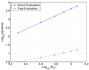
Fig. 1: The log-log (in base $10$) plot of the CPU time (in seconds) versus the total number of time steps $N_{T}$ for Application I. Here $N_{S}=30$ and $\alpha=0.5$.

3.3 Numerical Results

To test the convergence rates of the new scheme, we take the computational domain $\Omega_{i}=[0,\pi]$, and set

$$f(x,t)=\begin{cases}\Gamma(4+\alpha)x^{4}(\pi-x)^{4}\exp(-x)t^{3}/6-x^{2}(\pi-x)^{2}\{t^{3+\alpha}\exp(-x)\\ \left[x^{2}(56-16x+x^{2})-2\pi x(28-12x+x^{2})+\pi^{2}(12-8x+x^{2})\right]\\ +4(3\pi^{2}-14\pi x+14x^{2})\},\quad(x,t)\in\Omega_{i},\\ 0,\quad(x,t)\notin\Omega_{i},\end{cases}$$

$$u_{0}(x)=\begin{cases}x^{4}(\pi-x)^{4},\quad(x,t)\in\Omega_{i},\\ 0,\quad(x,t)\notin\Omega_{i}.\end{cases}$$

It is known that the IVP (37)–(39) has the exact solution given by the formula

$$u(x,t)=x^{4}(\pi-x)^{4}\left[\exp(-x)t^{3+\alpha}+1\right],\quad(x,t)\in\Omega_{i}\times(0,T].$$ (72)

To illustrate the performance of the numerical scheme, we define the maximum norm of the error and the convergence rates with respect to temporal and spatial sizes, respectively by the formulas

$$E(h,\Delta t)=\sqrt{\Delta t\sum_{k=1}^{N}\left\|e^{k}\right\|_{\infty}^{2}},\quad r_{t}=\log_{2}\frac{E(h,\Delta t)}{E(h,\Delta t/2)},\quad r_{s}=\log_{2}\frac{E(h,\Delta t)}{E(h/2,\Delta t)},$$

where the error $e^{k}$ is measured against the exact solution (72).

First, we check the convergence rate of the new scheme in time. We fix the spatial mesh size $h=\frac{\pi}{20000}$ and refine the temporal mesh size $\Delta t$ from $\frac{1}{10}$ to $\frac{1}{160}$. Obviously, $h$ is chosen so small that the error due to spatial discretization is negligible. The precision for the sum-of-exponentials approximation for the convolution kernel is set to $\varepsilon=10^{-7}$. Table 2 shows the numerical results for two different fractional values: $\alpha=0.2$ and $\alpha=0.5$. Next, we fix the temporal mesh size $\Delta t=\frac{1}{30000}$ so that the error due to temporal discretization is neglible. We then change the spatial step size $h$ from $\frac{\pi}{10}$ to $\frac{\pi}{160}$ to check the convergence order of the new scheme in space. Table 3 shows the numerical results for $\alpha=0.2$ and $\alpha=0.5$. Table 2 shows that the convergence order in time is ${O}(\Delta t^{2-\alpha})$ for both the direct scheme (46)-(47) and our fast scheme (50)-(51). While Table 3 shows that the convergence order in space is ${O}(h^{2})$ for both the direct scheme and our fast scheme.

To demonstrate the complexity of the two schemes, we plot in Fig 1 the CPU time of the two schemes in seconds. We observe that while the direct scheme scales like $O(N_{T}^{2})$, the CPU time increases almost linearly with the total number of time steps $N_{T}$ for the fast scheme. There is a significant speed-up in fast scheme as compared with the direct scheme even for $N_{T}$ of modest size.

4 Application II: Nonlinear Fractional Diffusion Equation

Consider now the initial value problem of the nonlinear fractional diffusion equation of the form

$${}_{0}^{C}\!D_{t}^{\alpha}u(x,t) =u_{xx}+f(u),$$ (73)

$$u(x,0) =u_{0}(x).$$

This problem has rich applications. When $f(u)=-u(1-u)$, (73) is the Fisher equation, which is used to model the spatial and temporal propagation of a virile gene in an infinite medium [14], the chemical kinetics [41], flame propagation [16], and many other scientific problems [43]. When $f(u)=-0.1u(1-u)(u-0.001)$, (73) is the time-fractional Huxley equation, which is used to describe the transmission of nerve impulses [15, 45] with many applications in biology and the population genetics in circuit theory [51].

When the initial data $u_{0}(x)$ is compactly supported on $\Omega_{i}=[x_{l},x_{r}]$, the following finite difference scheme with artificial boundary conditions imposed on two end points has been proposed in [36] to solve the problem (73)

$${{}^{C}_{0}}\mathbb{D}_{t}^{\alpha}U_{i}^{n}=\delta_{x}^{2}U_{i}^{n}+f(U_{i}^{n-1}),\qquad\qquad\qquad 1\leq i\leq M-1,$$ (74)

$$(\tilde{\delta}_{x}+3s_{0}^{\frac{\alpha}{2}}){{}^{C}_{0}}\mathbb{D}_{t}^{\alpha}U_{M-1}^{n}+(3s^{\alpha}_{0}\tilde{\delta}_{x}+s_{0}^{\frac{3\alpha}{2}}){U_{M-1}^{n}}=(\tilde{\delta}_{x}+3s_{0}^{\frac{\alpha}{2}})f(U_{M-1}^{n-1}),$$ (75)

$$(\tilde{\delta}_{x}-3s_{0}^{\frac{\alpha}{2}}){{}^{C}_{0}}\mathbb{D}_{t}^{\alpha}U_{1}^{n-1}+(3s^{\alpha}_{0}\tilde{\delta}_{x}-s_{0}^{\frac{3\alpha}{2}}){U_{1}^{n-1}}=(\tilde{\delta}_{x}-3s_{0}^{\frac{\alpha}{2}})f(U_{1}^{n-1}).$$ (76)

Under the assumption that $f(u)\in C^{2}([0,T])$, it has been shown in [36] that the scheme (74) the convergence rate of ${O}(h^{2}+\Delta t)$ in $L_{\infty}$ norm, defined by $\left\|e\right\|_{\infty}=\max\limits_{0\leq i\leq M}\left|e_{i}\right|$. With the L1-approximation ${{}^{C}_{0}}\mathbb{D}_{t}^{\alpha}$ replaced by our fast evaluation scheme ${{}^{FC}_{0}}\mathbb{D}_{t}^{\alpha}$, we obtain a fast scheme for solving (73), which is as follows:

$${{}^{FC}_{0}}\mathbb{D}_{t}^{\alpha}U_{i}^{n}=\delta_{x}^{2}U_{i}^{n}+f(U_{i}^{n-1}),\qquad\qquad\qquad 1\leq i\leq M-1,$$ (77)

$$(\tilde{\delta}_{x}+3s_{0}^{\frac{\alpha}{2}}){{}^{FC}_{0}}\mathbb{D}_{t}^{\alpha}U_{M-1}^{n}+(3s^{\alpha}_{0}\tilde{\delta}_{x}+s_{0}^{\frac{3\alpha}{2}}){U_{M-1}^{n}}=(\tilde{\delta}_{x}+3s_{0}^{\frac{\alpha}{2}})f(U_{M-1}^{n-1}),$$ (78)

$$(\tilde{\delta}_{x}-3s_{0}^{\frac{\alpha}{2}}){{}^{FC}_{0}}\mathbb{D}_{t}^{\alpha}U_{1}^{n-1}+(3s^{\alpha}_{0}\tilde{\delta}_{x}-s_{0}^{\frac{3\alpha}{2}}){U_{1}^{n-1}}=(\tilde{\delta}_{x}-3s_{0}^{\frac{\alpha}{2}})f(U_{1}^{n-1}).$$ (79)

4.1 Numerical Examples

We will give two examples - the Fisher equation and the Huxley equation to illustrate the performance of our scheme. For both examples, in order to investigate the convergence orders of our scheme, the reference solution is computed over a large interval $\Omega_{r}=[-12,12]$ with very small mesh sizes $h=2^{-10}$, and $\Delta t=2^{-14}$. We then set $\Omega_{i}=[-6,6]$ and the precision for the sum-of-exponentials approximation of the convolution kernel to $\varepsilon=10^{-9}$. The temporal step size is fixed at $\Delta t=2^{-14}$ when testing the order of convergence in space; and the spatial step size is fixed at $h=2^{-10}$ when testing the order of convergence in time.

Example 1.

We consider the time fractional Fisher equation

$$_{0}^{C}\!{D}_{t}^{\alpha}u(x,t)=u_{xx}-u(1-u),~{}~{}0<t\leq 1$$ (80)

with the double Gaussian initial value $u(x,0)=\exp(-10(x-0.5)^{2})+\exp(-10(x+0.5)^{2})$. Tables 4 and 5 present the numerical results for $\alpha=0.2,\ 0.5$, which show that our fast scheme (77)-(79) has the same convergence order ${O}(h^{2}+\Delta t)$ in $L_{\infty}$ norm as the direct scheme (74)-(76), but takes much less computational time.

Table 4: The errors and convergence orders in time for the fractional Fisher equation (80) with fixed spatial step size $h=2^{-10}$.

$\Delta t$	$\alpha=0.2$						$\alpha=0.5$
	Fast scheme			Direct scheme			Fast scheme			Direct scheme
	$\left\|e^{n}\right\|_{\infty}$	$r_{t}$		$\left\|e^{n}\right\|_{\infty}$	$r_{t}$		$\left\|e^{n}\right\|_{\infty}$	$r_{t}$		$\left\|e^{n}\right\|_{\infty}$	$r_{t}$
$1/10$	8.601e-04	1.02		8.601e-04	1.02		2.194e-03	1.09		2.194e-03	1.09
$1/20$	4.243e-04	1.01		4.243e-04	1.01		1.030e-03	1.06		1.030e-03	1.06
$1/40$	2.104e-04	1.01		2.104e-04	1.01		4.934e-04	1.04		4.934e-04	1.04
$1/80$	1.046e-04			1.046e-04			2.392e-04			2.392e-04

Table 5: The errors, convergence orders in space, and CPU time for the fractional Fisher equation (80) with fixed temporal step size $\Delta t=2^{-14}$.

$h$	$\alpha=0.2$						$\alpha=0.5$
	Fast scheme			Direct scheme			Fast scheme			Direct scheme
	$\left\|e^{n}\right\|_{\infty}$	$r_{s}$		$\left\|e^{n}\right\|_{\infty}$	$r_{s}$		$\left\|e^{n}\right\|_{\infty}$	$r_{s}$		$\left\|e^{n}\right\|_{\infty}$	$r_{s}$
$1/80$	8.196e-04	1.96		8.196e-04	1.96		6.045e-04	1.97		6.045e-04	1.97
$1/160$	2.112e-04	2.01		2.112e-04	2.01		1.547e-04	2.01		1.547e-04	2.01
$1/320$	5.246e-05	2.00		5.246e-05	2.00		3.842e-05	2.00		3.842e-05	2.00
$1/640$	1.316e-05			1.316e-05			9.649e-06			9.649e-06
CPU(s)	38.80			1071.91			40.22			850.58

Example 2.

We consider the fractional Huxley equation

$$_{0}^{C}\!{D}_{t}^{\alpha}u(x,t)=u_{xx}-0.1u(1-u)(u-0.001),~{}\quad 0<t\leq 1$$ (81)

with the double Gaussian initial value $u(x,0)=\exp(-10(x-0.5)^{2})+\exp(-10(x+0.5)^{2})$. Tables 6 and 7 present the numerical results for $\alpha=0.2,\ 0.5$, which show that our fast scheme (77)-(79) has the same convergence order ${O}(h^{2}+\Delta t)$ in $L_{\infty}$ norm as the direct scheme (74)-(76), but takes much less computational time.

To demonstrate the complexity of the two schemes, we plot in Fig. 2 the CPU time in seconds for both schemes. We observe that our fast scheme has almost linear complexity in $N_{T}$ and is much faster than the direct scheme.

Table 6: The errors and convergence orders in time for the fraction Huxley equation (81) with fixed spatial step size $h=2^{-10}$.

$\Delta t$	$\alpha=0.2$						$\alpha=0.5$
	Fast scheme			Direct scheme			Fast scheme			Direct scheme
	$\left\|e^{n}\right\|_{\infty}$	$r_{t}$		$\left\|e^{n}\right\|_{\infty}$	$r_{t}$		$\left\|e^{n}\right\|_{\infty}$	$r_{t}$		$\left\|e^{n}\right\|_{\infty}$	$r_{t}$
$1/10$	1.089e-03	1.04		1.089e-03	1.04		2.961e-03	1.06		2.961e-03	1.06
$1/20$	5.304e-04	1.02		5.304-04	1.02		1.418e-03	1.04		1.418e-03	1.04
$1/40$	2.614e-04	1.01		2.614e-04	1.01		6.896e-04	1.03		6.896e-04	1.03
$1/80$	1.294e-04			1.294e-04			3.379e-04			3.379e-04

Table 7: The errors, convergence orders in space, and CPU time for the fractional Huxley equation (81) with fixed temporal step size $\Delta t=2^{-14}$.

$h$	$\alpha=0.2$						$\alpha=0.5$
	Fast scheme			Direct scheme			Fast scheme			Direct scheme
	$\left\|e^{n}\right\|_{\infty}$	$r_{s}$		$\left\|e^{n}\right\|_{\infty}$	$r_{s}$		$\left\|e^{n}\right\|_{\infty}$	$r_{s}$		$\left\|e^{n}\right\|_{\infty}$	$r_{s}$
$1/80$	9.051e-04	1.96		9.051e-04	1.96		6.882e-04	1.98		6.882e-04	1.98
$1/160$	2.319e-04	2.01		2.319e-04	2.01		1.746e-04	2.01		1.746e-04	2.01
$1/320$	5.762e-05	2.00		5.762e-05	2.00		4.344e-05	2.00		4.344e-05	2.00
$1/640$	1.447e-05			1.447e-05			1.091e-05			1.091e-05
CPU(s)	38.69			1106.58			40.14			855.87

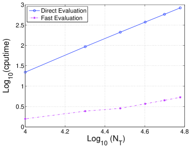
Fig. 2: The log-log (in base $10$) plot of the CPU time (in seconds) versus the total number of time steps $N_{T}$ for two schemes. Here $N_{S}=80$ and $\alpha=0.5$. The left panel shows the results for the Fisher equation, and the right panel shows the results for the Huxley equation.

5 Conclusions

We have developed a fast algorithm for the evaluation of the Caputo fractional derivative ${}_{0}^{C}\!D_{t}^{\alpha}f(t)$ for $0<\alpha<1$. The algorithm relies on an efficient sum-of-exponentials approximation for the convolution kernel $t^{-1-\alpha}$ with the absolute error $\varepsilon$ over the interval $[\Delta t,T]$. Specifically, we have shown that the number of exponentials needed in the approximation is of the order $O\left(\log\frac{1}{\varepsilon}\left(\log\log\frac{1}{\varepsilon}+\log\frac{T}{\Delta t}\right)+\right.$ $\left.\log\frac{1}{\Delta t}\left(\log\log\frac{1}{\varepsilon}+\log\frac{1}{\Delta t}\right)\right)$, which removes the term $O\left(\log^{2}\frac{1}{\varepsilon}\right)$ in [7, 37]. The resulting algorithm has nearly optimal complexity in both CPU time and storage.

We then applied our fast evaluation scheme of the Caputo derivative to solve the fractional diffusion equations. We first demonstrated that it is straightforward to incorporate our fast algorithm into the existing finite difference schemes for solving the fractional diffusion equations. We then proved a prior estimate about the solution of our new FD scheme which leads to the stability of the new scheme. We also presented a rigorous error bound for the new scheme. Finally, the numerical results on linear and nonlinear fraction diffusion equations show that our new scheme has the same order of convergence as the existing standard FD schemes, but with nearly optimal complexity in CPU time and storage.

Our work can be extended along several directions. First, it is straightforward to design high order schemes for the evaluation of fractional derivatives. Second, one may develop fast high-order algorithms for solving fractional PDEs which contains fractional derivatives in both time and space when the current scheme is combined with other existing schemes [10, 11, 12, 28]. Third, efficient and stable artificial boundary conditions can be designed using similar techniques in [27] for solving fractional PDEs in high dimensions. These issues are currently under investigation and the results will be reported on a later date.

Appendix A The Proof of Lemma 8

Proof.

Applying the definition (27) of the fast evaluation scheme and the Cauchy-Schwarz inequality, we have

$$({{}^{FC}_{0}}\mathbb{D}_{t}^{\alpha}g^{k})g^{k} =\frac{1}{\Delta t^{\alpha}\Gamma(1-\alpha)}\bigg{(}\frac{1}{1-\alpha}(g^{k})^{2}-(\frac{\alpha}{1-\alpha}+a_{0})g^{k-1}g^{k}$$

$$\quad-\sum_{l=1}^{k-2}(a_{k-l-1}+b_{k-l-2})g^{l}g^{k}-(b_{k-2}+\frac{1}{2k^{\alpha}})g^{0}g^{k}\bigg{)}$$

$$\geq\frac{1}{\Delta t^{\alpha}\Gamma(1-\alpha)}\left[\bigg{(}\frac{2-\alpha}{2(1-\alpha)}-\frac{1}{2}\sum_{l=0}^{k-2}(a_{l}+b_{l})-\frac{1}{k^{\alpha}}\bigg{)}(g^{k})^{2}\right.$$

$$\quad\left.-\frac{1}{2}(\frac{\alpha}{1-\alpha}+a_{0})(g^{k-1})^{2}-\frac{1}{2}\sum_{l=1}^{k-2}(a_{k-l-1}+b_{k-l-2})(g^{l})^{2}\right.$$

$$\quad\left.-\frac{1}{2}(b_{k-2}+\frac{1}{k^{\alpha}})(g^{0})^{2}\bigg{)}\right].$$ (82)

Summing the above inequality from $k=1$ to $n$, we obtain

$$\Delta t\sum_{k=1}^{n}({{}^{FC}_{0}}\mathbb{D}_{t}^{\alpha}g^{k})g^{k}\geq\frac{\Delta t^{1-\alpha}}{\Gamma(1-\alpha)}\left[\sum_{k=2}^{n}\bigg{(}\frac{1}{1-\alpha}-\frac{\alpha}{2(1-\alpha)}-\frac{1}{2}\sum_{l=0}^{k-2}(a_{l}+b_{l})-\frac{1}{2k^{\alpha}}\bigg{)}(g^{k})^{2}\right.$$

$$-\left.\sum_{k=2}^{n}\bigg{(}\frac{\alpha}{2(1-\alpha)}+\frac{a_{0}}{2}\bigg{)}(g^{k-1})^{2}-\frac{1}{2}\sum_{k=2}^{n}\sum_{l=1}^{k-2}\bigg{(}a_{k-l-1}+b_{k-l-2}\bigg{)}(g^{l})^{2}\right.$$

$$+\left.\frac{1}{2(1-\alpha)}(g^{1})^{2}-\frac{1}{2(1-\alpha)}(g^{0})^{2}-\frac{1}{2}\sum_{k=2}^{n}\bigg{(}b_{k-2}+\frac{1}{k^{\alpha}}\bigg{)}(g^{0})^{2}\right]$$

$$=\frac{\Delta t^{1-\alpha}}{\Gamma(1-\alpha)}\sum_{k=1}^{n}\bigg{(}C_{k}(g^{k})^{2}-C_{0}(g^{0})^{2}\bigg{)},$$ (83)

where the coefficients $C_{k}$ ($k=0,1,\cdots,n$) are given by the formula

$$C_{k}=\left\{\begin{array}[]{ll}\frac{1}{2(1-\alpha)}+\frac{1}{2}\sum\limits_{k=2}^{n}(b_{k-2}+\frac{1}{k^{\alpha}}),&\;k=0,\\ \frac{1}{2}-\frac{1}{2}\sum\limits_{l=0}^{n-2}(a_{l}+b_{l})+\frac{1}{2}b_{n-2},&\;k=1,\\ 1-\frac{1}{2}\sum\limits_{l=0}^{k-2}(a_{l}+b_{l})-\frac{1}{2k^{\alpha}}-\frac{1}{2}\sum\limits_{l=0}^{n-k-1}(a_{l}+b_{l})+\frac{1}{2}b_{n-k-1},&\;2\leq k<n,\\ \frac{2-\alpha}{2(1-\alpha)}-\frac{1}{2}\sum\limits_{l=0}^{k-2}(a_{l}+b_{l})-\frac{1}{2k^{\alpha}},&\;k=n.\end{array}\right.$$ (88)

From (6), we have the estimate

$$\frac{1}{t^{1+\alpha}}-\varepsilon\leq\sum_{j=1}^{N_{\text{exp}}}\omega_{j}{e^{-s_{j}t}}\leq\frac{1}{t^{1+\alpha}}+\varepsilon.$$ (89)

It is also straightforward to verify that

$$\sum_{l=0}^{k-2}(a_{l}+b_{l})=\alpha\Delta t^{\alpha}\int_{\Delta t}^{k\Delta t}\sum_{j=1}^{N_{\text{exp}}}\omega_{j}{e^{-s_{j}t}}\mathrm{d}t.$$ (90)

Combining (89) and (90), we obtain

$$(1-\frac{1}{k^{\alpha}})-\alpha\Delta t^{\alpha}t_{k-1}\varepsilon\leq\sum_{l=0}^{k-2}(a_{l}+b_{l})\leq(1-\frac{1}{k^{\alpha}})+\alpha\Delta t^{\alpha}t_{k-1}\varepsilon,$$ (91)

Substituting (91) into (88) yields the following estimates

$$\left\{\begin{array}[]{ll}C_{0}&\leq\frac{n^{1-\alpha}}{(1-\alpha)}+\alpha\Delta t^{\alpha}t_{n-1}\varepsilon,\\ C_{1}&\geq\frac{1}{2}-\frac{1}{2}\sum\limits_{l=0}^{n-2}(a_{l}+b_{l})\geq\frac{1}{2n^{\alpha}}-\alpha\Delta t^{\alpha}t_{n-1}\varepsilon,\\ C_{k}&=1-\frac{1}{2}\sum\limits_{l=0}^{k-2}(a_{l}+b_{l})-\frac{1}{2k^{\alpha}}-\frac{1}{2}\sum\limits_{l=0}^{n-k-1}(a_{l}+b_{l})+\frac{1}{2}b_{n-k-1}\\ &\geq\frac{1}{2n^{\alpha}}-\alpha\Delta t^{\alpha}t_{n-1}\varepsilon,\quad 2\leq k\leq n-1,\\ C_{n}&\geq\frac{2-\alpha}{2(1-\alpha)}-\sum\limits_{l=0}^{n-2}(a_{l}+b_{l})-\frac{1}{2n^{\alpha}}\geq\frac{1}{2n^{\alpha}}-\alpha\Delta t^{\alpha}t_{n-1}\varepsilon.\\ \end{array}\right.$$ (97)

Combining (A) and (97), we obtain Lemma 8. ∎

References

• [1] B. Alpert, L. Greengard, and T. Hagstrom, Rapid evaluation of nonreflecting boundary kernels for time-domain wave propagation, SIAM J. Numer. Anal., 37 (2000), 1138–1164.
• [2] B. Alpert, L. Greengard, and T. Hagstrom, Nonreflecting Boundary Conditions for the Time-Dependent Wave Equation, J. Comput. Phys. 180 (2002), 270–296.
• [3] A. A. Awotunde, R. A. Ghanam, and N. Tatar, Artificial boundary condition for a modified fractional diffusion problem, Boundary Value Problems, (1) 2015, 1–17.
• [4] H. Brunner, H. Han, and D. Yin, Artificial boundary conditions and finite difference approximations for a time-fractional diffusion-wave equation on a two-dimensional unbounded spatial domain, J. Comput. Phys., 276 (2014), 541–562.
• [5] G. Beylkin and L. Monzón, On generalized Gaussian quadratures for exponentials and their applications, Appl. Comput. Harmon. Anal., 12(3) (2002), 332–373.
• [6] G. Beylkin and L. Monzón, On approximation of functions by exponential sums, Appl. Comput. Harmon. Anal., 19 (2005), 17–48.
• [7] G. Beylkin and L. Monzón, Approximation by exponential sums revisited, Appl. Comput. Harmon. Anal., 28 (2010), 131–149.
• [8] H.Brunner, H.Han, and D.Yin, The maximum principle for time-fractional diffusion equations and its application, to appear in SIAM J. Numer. Anal., 2015..
• [9] J. Cao and C. Xu, A high order scheme for the numerical solution of the fractional ordinary differential equations, J. Comput. Phys., 238 (2013), 154–168.
• [10] C. Chen, F. Liu, V. Anh, and I. Turner, Numerical methods for solving a two-dimensional variable-order anomalous subdiffusion equation, Math. Comp., 81 (2012), 345–366.
• [11] M. Cui, Compact finite difference method for the fractional diffusion equation, J. Comput. Phys., 228 (2009), 7792–7804.
• [12] M. Cui, Compact alternating direction implicit method for two-dimensional time fractional diffusion equation, J. Comput. Phys., 231 (2012), 2621–2633.
• [13] J.R. Dea, Absorbing boundary conditions for the fractional wave equation, Appl. Math. Comput., 219 (2013), 9810–9820.
• [14] R. A. Fisher, The wave of advance of advantageous genes, Ann. Eugene 7 (1937), 335–369.
• [15] R. Fitzhugh, Impulse and physiological states in models of nerve membrane, Biophys. J, 1 (1961), 445–466.
• [16] D. A. Frank, Diffusion and heat exchange in chemical kinetics, Princeton University Press, Princeton, NJ, USA.
• [17] G. H. Gao, Z. Z. Sun, and Y. N. Zhang, A finite difference scheme for fractional sub-diffusion equations on an unbounded domain using artificial boundary conditions, J. Comput. Phys., 231 (2012), 2865–2879.
• [18] G. H. Gao and Z. Z. Sun, The finite difference approximation for a class of fractional sub-diffusion equations on a space unbounded domain, J. Comput. Phys., 236 (2013), 443–460.
• [19] G. H. Gao and Z. Z. Sun, A compact finite difference scheme for the fractional sub-diffusion equations, J. Comput. Phys., 230 (2011), 586–595.
• [20] G. H. Gao and Z. Z. Sun, A new fractional numerical differentiation formula to approximate the Caputo fractional derivative and its applications, J. Comput. Phys., 259 (2014), 33–50.
• [21] R. Ghaffari and S. M. Hosseini, Obtaining artificial boundary conditions for fractional sub-diffusion equation on space two-dimensional unbounded domains, Comput. Math. Appl., 68 (2014) 13–26.
• [22] L. Greengard and P. Lin, Spectral Approximation of the Free-Space Heat Kernel, Appl. Comput. Harmon. Anal., 9 (2000), 83–97.
• [23] L. Greengard and J. Strain, A Fast Algorithm for the Evaluation of Heat Potentials, Comm. Pure Appl. Math., 43 (1990), 949–963.
• [24] H. Han and X. Wu, Artificial Boundary Method, Tsinghua Univ. Press, 2013.
• [25] S. Jiang, Fast Evaluation of the Nonreflecting Boundary Conditions for the Schrödinger Equation, Ph.D. thesis, Courant Institute of Mathematical Sciences, New York University, New York, 2001.
• [26] S. Jiang and L. Greengard, Fast Evaluation of Nonreflecting Boundary Conditions for the Schrödinger Equation in One Dimension, Comput. Math. Appl. 47 (2004), no. 6-7, 955–966.
• [27] S. Jiang and L. Greengard, Efficient representation of nonreflecting boundary conditions for the time-dependent Schrödinger equation in two dimensions, Comm. Pure Appl. Math., 61 (2008), 261–288.
• [28] S. Jiang, L. Greengard, and W. Bao, Fast and accurate evaluation of nonlocal Coulomb and dipole-dipole interactions via the nonuniform FFT, SIAM J. Sci. Comput., 36 (2014), no. 5, B777-B794.
• [29] S. Jiang, L. Greengard, and S. Wang, Efficient sum-of-exponentials approximations for the heat kernel and their applications, Adv. Comput. Math., 41 (2015), no. 3, 529–551.
• [30] A. Kilbas, H. Srivastava, J. Trujillo, Theory and Applications of Fractional Differential Equations, Elesvier Science and Technology, Boston, 2006.
• [31] T. Langlands and B. Henry, Fractional chemotaxis diffusion equations, Phys. Rev. E 81 (2010), 051102.
• [32] T. Langlands and B. Henry, The accuracy and stability of an implicit solution method for the fractional diffusion equation, J. Comput. Phys., 205 (2005), 719–736.
• [33] S. Lei and H. Sun, A circulant preconditioner for fractional diffusion equations, J. Comput. Phys., 242, (2013), 715–725.
• [34] C. Li, W. Deng, and Y. Wu, Numerical analysis and physical simulations for the time fractional radial diffusion equation, Comput. Math. Appl., 62 (2011), 1024–1037.
• [35] C. Li, A. Chen, and J. Ye, Numerical approaches to fractional calculus and fractional ordinary differential equation, J. Comput. Phys., 230 (2011), 3352–3368.
• [36] D. Li and J. Zhang, Efficient implementation to numerically solve the nonlinear time fractional parabolic problems on unbounded spatial domain, submitted.
• [37] J. Li, A fast time stepping method for evaluating fractional integrals, SIAM J. Sci. Comput., 31 (2010), 4696–4714.
• [38] Y. Lin and C. Xu, Finite difference/spectral approximations for the time-fractional diffusion equation, J. Comput. Phys., 225 (2007), 1533–1552.
• [39] Y. Lin, X. Li, and C. Xu, Finite difference/spectral approximations for the fractional cable equation, Math. Comp., 80 (2011), 1369–1396.
• [40] Y. Lin and C. Xu, Finite difference/spectral approximations for time-fractional diffusion equation, J. Comput. Phys., 225 (2007), 1533–1552.
• [41] W. Malflict, Solitary wave solutions of nonlinear wave equations, Am. J. Phys, 60 (1992), 650–654.
• [42] W. McLean, Fast summation by interval clustering for an evolution equation with memory, SIAM J. Numer. Anal., 34(6) (2012), 3039–3056.
• [43] M. Merdan, Solutions of time-fractional reaction-diffusion equation with modified Riemann-Liouville derivative, Int. J. Phys. Sci, 7 (2012), 2317–2326.
• [44] R. Metzler and J. Klafter, The random walks guide to anomalous diffusion: a fractional dynamics approach, Phys. Rep. 339 (2000).
• [45] J.S. Nagumo. S. Arimoto, and S. Yoshizawa, An active pulse transmission line simulating nerve axon, Proc IRE, 50 (1962), 2061–2070.
• [46] Z. Odibat, Approximations of fractional integrals and Caputo fractional derivatives, Appl. Math. Comput., 178 (2006), 527–533.
• [47] K.B. Oldham and J. Spanier, The Fractional Calculus, Academic Press, New York, 1974.
• [48] F. W. J. Olver, D. W. Lozier, R. F. Boisvert, and C. W. Clark, editors. NIST Handbook of Mathematical Functions, Cambridge University Press, New York, NY, 2010.
• [49] H. Pang and H. Sun, Multigrid method for fractional diffusion equations, J. Comput. Phys., 231 (2012), 693–703.
• [50] I. Podlubny, Fractional Differential Equations, Academic Press, San Diego, 1999.
• [51] M. Shih, E. Momoniat, and F. M. Mahomed, Approximate conditional symmetries and approximate solutions of the perturbed Fitzhugh-Nagumo equation, J. Math. Phys, 46 (2005), 023503.
• [52] Z. Sun and X. Wu, A fully discrete difference scheme for a diffusion-wave system, Appl. Numer. Math., 56 (2006), 193–209.
• [53] H. Wang, K. Wang, and T. Sircar, A direct $O(Nlog^{2}N)$ finite difference method for fractional diffusion equations, J. Comput. Phys., 229 (2010), 8095–8104.
• [54] H. Wang and S.B. Treena, A Fast Finite Difference Method for Two-Dimensional Space-Fractional Diffusion Equations, SIAM J. Sci. Comput., 34 (2012), 2444–2458.
• [55] K. Xu and S. Jiang, A Bootstrap Method for Sum-of-Poles Approximations, J. Sci. Comput., 55 (2013), 16–39.
• [56] C. Zheng, Approximation, stability and fast evaluation of exact artificial boundary condition for one-dimensional heat equation, J. Comput. Math., 25 (2007), 730–745.