Loop-nodal and Point-nodal Semimetals in Three-dimensional Honeycomb Lattices

Abstract

Honeycomb structure has a natural extension to the three dimensions. Simple examples are hyperhoneycomb and stripy-honeycomb lattices, which are realized in $\beta$-Li₂IrO₃ and $\gamma$-Li₂IrO₃, respectively. We propose a wide class of three-dimensional (3D) honeycomb lattices which are loop-nodal semimetals. Their edge states have intriguing properties similar to the two-dimensional honeycomb lattice in spite of dimensional difference. Partial flat bands emerge at the zigzag or beard edge of the 3D honeycomb lattice, whose boundary is given by the Fermi loop in the bulk spectrum. Analytic solutions are explicitly constructed for them. On the other hand, perfect flat bands emerge in the zigzag-beard edge or when the anisotropy is large. All these 3D honeycomb lattices become strong topological insulators with the inclusion of the spin-orbit interaction. Furthermore, point-nodal semimetals may be realized in the presence of both the antiferromagnetic order and the spin-orbit interaction.

Honeycomb lattice is materialized naturally in graphene and in related materials, which presents one of the most active fields of condensed matter physics. The Fermi surface is zero dimensional, given by the $K$ and $K^{\prime}$ points, though in general the dimension of the Fermi surface is $D-1$ for the $D$-dimensional system. It may be called a point-nodal semimetal with the Dirac cone. A nanoribbon made of honeycomb lattice has interesting properties such as zero-energy flat bands connecting the $K$ and $K^{\prime}$ pointsKlein ; Fujita ; EzawaGNR . Perfect flat bands are generated when the $K$ and $K^{\prime}$ points are shifted and merged by introducing anisotropy in the hoppingWunsch ; Pere ; Monta , which is realized in phosphorenePhos . A natural question is whether there are similar properties in the three dimensions.

Honeycomb structure has a natural extension to the three dimensions. Examples are hyperhoneycombTakagi ; Biffin ; Modic and stripy-honeycombModic lattices, being realized in $\beta$-Li₂IrO₃ and $\gamma$-Li₂IrO₃, respectively. A series of three-dimensional (3D) honeycomb lattices named harmonic honeycomb latticesModic have also been proposed. They attracts much attentionLee ; LeeAF ; Mullen ; Nasu ; Kimchi ; LeeO ; Nasu2 ; Hermanns recently. It has been arguedLee ; Mullen that the hyperhoneycomb lattice is a loop-nodal semimetal where the Fermi surface forms a loop (which we call a Fermi loop). Furthermore, the system becomes a topological insulator by introducing a spin-orbit interactionLee (SOI). Various antiferromagnetic order is reported in the hyperhoneycomb latticeLeeAF ; LeeO ; Kimchi ; Kimchi2 . Similar Fermi loops have been predicted in other systemsPhilip ; Xie ; Yu ; Kim based on first-principles calculation.

In this Letter, we propose a wide class of 3D honeycomb lattices which are loop-nodal semimetals. We first analyze the edge states of nanofilms made of them. Flat-band edge states emerge at the zigzag or beard edge termination, which are reminiscence of the edge states of the honeycomb system. We derive an analytic form of the wave function by the recursion method. The boundary of the zero-energy states is given by the Fermi loop in the bulk spectrum. It is shown that the perfect flat band is generated over the whole region of the Brillouin zone by two methods: One is terminating the sample with the zigzag and beard edges; The other is increasing the anisotropy, where the Fermi loop shrinks and disappears. All these 3D honeycomb lattices become strong topological insulators in the presence of the spin-orbit interaction. Furthermore, a point-nodal semimetal may be generated together with a Dirac cone in the additional presence of the antiferromagnetic order.

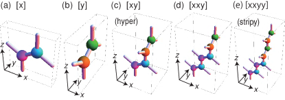
Figure 1: Unit cells of various honeycomb lattices. The unit cell $[\alpha_{1}]$ of the honeycomb lattice placed on (a) the $xz$-plane and (b) the $yz$-plane. We use these building blocks to construct 3D honeycomb lattices. (c,d,e) Typical examples of unit cells $[\alpha_{1}\alpha_{2}\cdots\alpha_{N}]$ made by sewing the above building blocks.

Lattice structure and model: Honeycomb lattice is a bipartite system. The unit cell contains two vertices (atoms) and five links (bonds) making the angle $2\pi/3$ between the neighboring ones with certain links being identified on one plane. We prepare two sets placed on the $xz$ plane and the $yz$ plane, and refer to them as the building blocks $[x]$ and $[y]$, respectively: See illustration in Fig.1(a) and (b). We propose a class of 3D honeycomb lattices by sewing these two building blocks in such a way that all atoms in one unit cell are connected with a single path tending to the $z$ direction [Fig.1(c), (d) and (e)].

Let us first consider the unit cell containing $4$ atoms. It is uniquely given by $[xy]$ if we start with $[x]$. Note that $[xx]$ is equivalent to $[x]$. In general, the unit cell containing $N$ building blocks is represented by $[\alpha_{1}\alpha_{2}\cdots\alpha_{N}]$, where $\alpha_{n}=x$ or $y$. There exist the cyclic symmetry; namely, two unit cells $[\alpha_{1}\alpha_{2}\cdots\alpha_{N-1}\alpha_{N}]$ and $[\alpha_{2}\alpha_{3}\cdots\alpha_{N}\alpha_{1}]$ are equivalent. Furthermore, $[\alpha_{1}\alpha_{2}\cdots\alpha_{N}]$ and $[\bar{\alpha}_{1}\bar{\alpha}_{2}\cdots\bar{\alpha}_{N}]$ are equivalent, where $\bar{\alpha}_{n}=y$ $(x)$ if $\alpha_{n}=x$ $(y)$. The simplest 3D honeycomb lattice is generated by the unit cell $[xy]$, which has been named the hyperhoneycomb lattice. The next simplest one is $[xxy]$. Then, we have $[xxyy]$, which generates the stripy-honeycomb lattice. The type of lattices with the unit cell $[x\cdots xy\cdots y]$ in sequential order of $x$ and $\ y$ has been named the harmonic honeycomb lattice when the numbers of $x$’s and $y$’s are equal.

Loop-nodal semimetal: We consider a free-electron system hopping on the 3D honeycomb lattice whose unit is $[\alpha_{1}\alpha_{2}\cdots\alpha_{N}]$. The Hamiltonian is given $H=\sum_{\langle i,j\rangle}t_{ij}c_{i}^{\dagger}c_{j},$ where $t_{ij}=t_{z}$ for the nearest neighbor hopping along the $z$ axis and $t_{ij}=t_{xy}$ for the other nearest-neighbor hopping and $c_{i}$ ($c_{i}^{\dagger}$) is the annihilation (creation) operator of the electron at the site $i$. In the momentum representation it is given by the $2N\times 2N$ matrixLee , $H_{2N}=\sum_{\boldsymbol{k}}c^{\dagger}(\boldsymbol{k})\hat{H}_{2N}(\boldsymbol{k})c(\boldsymbol{k}),$ with $H_{2n-1,2n}=f_{\alpha_{n}}$, $H_{2n,2n-1}=f_{\alpha_{n}}^{\ast}$, $H_{2n,2n+1}=f_{z}$, $H_{2n+1,2n}=f_{z}^{\ast}$, $H_{2N,1}=f_{z}$, $H_{1,2N}=f_{z}^{\ast}$ and all other elements being zero, where

$$f_{\alpha}=2t_{xy}e^{i\frac{k_{z}}{2}}\cos\frac{\sqrt{3}}{2}k_{\alpha},\qquad f_{z}=t_{z}e^{ik_{z}},$$ (1)

with $\alpha=x,y$.

The energy spectrum is determined by $\det\left(\lambda I-H\right)=0$. Especially, the zero-energy states are solutions of $\det H=0$, which is calculated as

$$\det H=|f_{z}^{\ast N}-\prod\limits_{n=1}^{N}f_{\alpha_{n}}|^{2}.$$ (2)

The solution is given by $k_{z}=0$ and

$$\cos^{N_{x}}\frac{\sqrt{3}}{2}k_{x}\cos^{N_{y}}\frac{\sqrt{3}}{2}k_{y}=(t_{z}/2t_{xy})^{N_{x}+N_{y}},$$ (3)

where $N_{x}$ $(N_{y})$ is the number of $x$’s ($y$’s) in $[\alpha_{1}\alpha_{2}\cdots\alpha_{N}]$. It represents a loop in the momentum space [Fig.2(a)]. Hence, all 3D honeycomb lattices in this class are loop-nodal semimetals. It follows that the Fermi surface exists only for $\left|t_{xy}/t_{z}\right|>1/2$, as agrees with the previous result for the case of the hyperhoneycomb latticeLee ; Mullen with $t_{xy}=t_{z}$.

We may illustrate the equi-energy surface of the hyperhoneycomb lattice in the momentum space for a typical value of $E$ in Fig.2(b). It shows a toroidal Fermi surface around the $\Gamma$ point ($\boldsymbol{k}=\boldsymbol{0}$). It shrinks to a 1D circle forming a Fermi loop at the half filling with $E=0$.

Analytic wave function of the zero-energy edge states: We first analyze the edge states of the 3D honeycomb lattice, whose edge is taken at $z=0$. The momentum $k_{x}$ and $k_{y}$ remain to be good quantum numbers. The wave function is constructed analytically with the aid of the recursive method as in the case of the honeycomb systemKohmoto . We define the wave function $\psi_{i}$ for the $i$-th sites counting from the bottom of the sample.

The wave functions of the zero-energy states must satisfy $H\psi=0$, which is explicitly given by

$$S_{\pm}\equiv t_{xy}(1+e^{i\sqrt{3}k_{\alpha_{n}}})\psi_{2n\pm 1}+t_{z}\psi_{2n\mp 1}=0,$$ (4)

for the odd sites of the zigzag ($S_{+}$) and beard ($S_{-}$) edges, and $\psi_{2n}=0$ for the even sites. The wave function can be solved recursively as

$$\psi_{2n+1}=\left(-\frac{t_{xy}}{t_{z}}\right)^{\pm n}\prod\limits_{j=1}^{n}(1+e^{i\sqrt{3}k_{\alpha_{j}}})^{\pm 1}\psi_{1}$$ (5)

for the zigzag ($+$) and beard ($-$) edges.

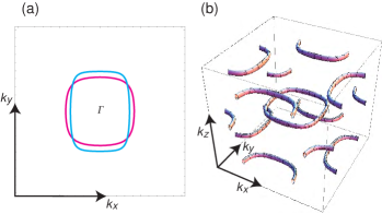
Figure 2: (a) Fermi loops with $N_{x}=N_{y}$ (magenta) and $N_{x}=4N_{y}$ (cyan), which appear in the $k_{x}k_{y}$ plane at $k_{z}=0$. We have set $t_{z}=t_{xy}=1$. (b) Bird’s eye’s view of the contour plot of the equi-energy surface with $N_{x}=N_{y}$ for $E=0.1t$ with $t=t_{xy}=t_{z}$ in a part of the extended Brillouin zone.

For the zero-energy state, the wave function must take the maximum value at the outermost edge sites and its absolute value must decrease as the site index $i$ increases. Otherwise, the wave function diverges inside the bulk and we cannot normalize it. This condition is given by

$$\cos^{N_{x}}\frac{\sqrt{3}}{2}k_{x}\cos^{N_{y}}\frac{\sqrt{3}}{2}k_{y}\lessgtr(t_{z}/2t_{xy})^{N_{x}+N_{y}}$$ (6)

for the zigzag edge ($<$) and for the beard edge ($>$). Accordingly, the zero-energy states emerge in the region whose boundary is the Fermi loop (3) in the bulk spectrum.

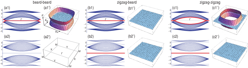
Figure 3: Band structures of nanofilms made of isotropic and anisotropic hyperhoneycomb lattices. Edge states are marked in red. (a1),(c1) Pertial flat bands appear for $|t_{z}|<2|t_{xy}|$ in the inner (outer) region of the Fermi loop when the both edges are terminated by the beard (zigzag) edge. (b) The perfect flat bands appear over the whole Brillouin zone irrespective to the value of $t_{z}$ and $t_{xy}$ when the edges are terminated by the zigzag and beard edges. (a2),(b2),(c2) The perfect flat bands appear for $|t_{z}|>2|t_{xy}|$ irrespective to the type of edge termination. We have set $t_{xy}=1,V=0,\lambda_{xy}=\lambda_{z}=0$. We have also set $t_{z}=1$ for (a1), (b1), (c1) (isotropic), and $t_{z}=2.5$ for (a2), (b2), (c2).

It follows from (5) that $\psi_{1}=1$ and $\psi_{i}=0$ for $i\geq 2$ at the M point ($k_{x}=k_{y}=\pi/\sqrt{3}$) for the zigzag edge, which represents the perfectly localized state corresponding to the perfectly localized state at the zigzag edge of the honeycomb lattice. Contrary to the zigzag edge states, there is no perfectly localized edge state in the beard edge states.

We proceed to consider a nanofilm where the width along the $z$ direction is finite. Both of the zigzag and beard edge terminations are possible depending on the position of the edges. For definiteness, we show the band structure of a nanofilm made of the hyperhoneycomb lattice in Fig.3. Flat bands emerge in the band structure, which are reminiscence of flat bands in the zigzag and beard edges in the honeycomb lattice. When the one edge is terminated by the zigzag edge and the other edge is terminated by the beard edge, the perfect flat bands emerge over the whole Brillouin zone [Fig.3(b)].

Anisotropic 3D honeycomb lattice: We next investigate how the edge states are modified by changing the transfer energy $t_{z}$ and $t_{xy}$. The ratio $t_{xy}/t_{z}$ can be tuned by applying uni-axial pressure. We show the band structure with (a) the zigzag-zigzag edges, (b) the zigzag-beard edges, and (c) the beard-beard edges in Fig.3 for typical values of $t_{xy}$ and $t_{z}$.

The flat band region shrinks as the $t_{z}/t_{xy}$ increases and disappears for $|t_{z}/t_{xy}|>2$ for the beard-beard edge [Fig.3(a)]. It is natural since there is no solution of $k_{x}$ and $k_{y}$ for $|t_{z}/t_{xy}|>2$ in eq.(6) with $<$. On the contrary, the flat band region expands as $t_{z}/t_{xy}$ increases and the whole region of the Brillouin zone becomes the perfect flat band for $|t_{z}/t_{xy}|>2$ for the zigzag-zigzag edge [Fig.3(b)]. This can be understood that the condition (6) with $>$ is satisfied irrespective of the values of $k_{x}$ and $k_{y}$ for $|t_{z}/t_{xy}|>2$.

These feature are reminiscence of the anisotropic 2D honeycomb latticeWunsch ; Pere ; Monta , where there are two different transfer energies $t_{1}$ and $t_{2}$. There are $K$ and $K^{\prime}$ points in the honeycomb lattice when $t_{1}=t_{2}$. These $K$ and $K^{\prime}$ points move by changing the ratio of the transfer energies $t_{2}/t_{1}$. When $\left|t_{2}/t_{1}\right|>2$ they merges resulting in an insulator, where the band dispersion is highly anisotropic. Phosphorene, monolayer black phosphorus, is understood in this picturePhos .

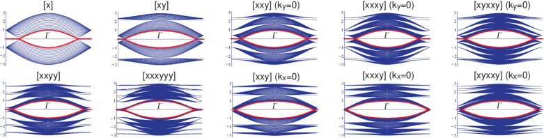
Figure 4: Band structures of nanofilms made of typical 3D-honeycomb lattices indexed by $[\alpha_{1}\alpha_{2}\cdots\alpha_{N}]$. Edge states are marked in red. All nanofilms have similar band structures near the Fermi level.

We have so far used the instance of the hyperhoneycomb lattices for illustration. Here we show the band structures of nanofilms made of various 3D honeycomb lattices in Fig.4. We find that the flat-band zero-energy edge states emerge in the same region of the hyperhoneycomb lattice although the high-energy band structure is different. We note that the band structure along the $k_{x}$ and $k_{y}$ directions are inequivalent for the 3D honeycomb lattice with $N_{x}\neq N_{y}$.

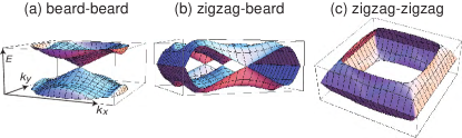
Figure 5: Band structure of a nanofilm with the SOI for (a) beard-beard edge, (b) zigzag-beard edge and (c) zigzag-zigzag edge. One (two) Dirac cones appear in the beard-beard (zigzag-beard) edge. We have set $\lambda_{xy}=\lambda_{z}=0.2t/2\sqrt{3}$ with $t=t_{xy}=t_{z}$.

Spin-orbit interaction: It has been shown for the hyperhoneycomb systemLee that the system turns into a strong topological insulator in the presence of the SOI. The Kane-Mele type spin-orbit interaction is given byKaneMele ; FuKaneMele ; Lee $H_{\lambda}=i\boldsymbol{v}_{ij}\cdot\boldsymbol{\sigma},$ with $\boldsymbol{v}_{ij}=v_{\text{KM}}\frac{\boldsymbol{r}_{ik}\times\boldsymbol{r}_{kj}}{\left|\boldsymbol{r}_{ik}\times\boldsymbol{r}_{kj}\right|},$where $v_{\text{KM}}$ is the strength of the spin-orbit interaction. We assume $v_{\text{KM}}=\lambda_{z}$ for the $z$-direction and $v_{\text{KM}}=\lambda_{xy}$ for the in-plane direction. We show how the flat-band edge states change by introducing the spin-orbit interaction. The resultant edge states are shown in Fig.5. The flat-band edge states are bent by the SOI and turn into the topological edge states. For example, the edge states are well described by the tetragonal-warped Dirac cone for the beard-beard edges. On the other hand, the shapes of the topological edge states are much different from the Dirac spectrum for the zigzag-zigzag and zigzag-beard edges.

Effective model: There are two bands near the Fermi energy for each spin. It is possible to solve these eigenstates $\psi_{\pm}$ explicitly as $H_{2N}\psi_{\pm}=\pm(2t_{xy}-t_{z})\psi_{\pm}$ with $\psi_{\pm}=(\pm 1,-1,\mp 1,1,\cdots)$ when $N$ is even. We derive the effective 4-band model with the SOI in order to describe the physics near the Fermi energy. By evaluating $\psi_{\pm}^{\dagger}H\psi_{\pm}$, we obtain the effective 4-band theory,

$$H_{\text{eff}}=d_{1}\tau_{z}+d_{2}\tau_{y}+(-W+\frac{2N_{x}}{N}\Lambda_{y}\sigma_{x}+\frac{2N_{y}}{N}\Lambda_{x}\sigma_{y})\tau_{x},$$ (7)

where

$$d_{1}+id_{2} =t_{z}e^{ik_{z}}-t_{xy}e^{-i\frac{k_{z}}{2}}\sum_{\alpha=x,y}\frac{2N_{\alpha}}{N}\cos\frac{\sqrt{3}k_{\alpha}}{2},$$ (8)

$$\Lambda_{\alpha} =\lambda_{z}\sin\sqrt{3}k_{\alpha}+2\lambda_{xy}\sin\frac{\sqrt{3}k_{\alpha}}{2}\cos\frac{3k_{z}}{2},$$ (9)

with $\alpha=x,y$, and $W=V+\boldsymbol{V}_{\text{AF}}\cdot\boldsymbol{\sigma}$. Here we have additionally included the staggered potential $V$ and the antiferromagnetic staggered potential $\boldsymbol{V}_{\text{AF}}$ between the two sublattices in the bipartite system [Fig.1].

The $\mathbb{Z}_{2}$ index: We calculate the $\mathbb{Z}_{2}$ index for $V=\left|\boldsymbol{V}_{\text{AF}}\right|=0$. There are the time-reversal symmetry and the inversion symmetry for $V=\left|\boldsymbol{V}_{\text{AF}}\right|=0$. The inversion symmetry operator is given by $P=\tau_{z}$ with $PH_{\text{eff}}(\boldsymbol{k})P^{-1}=H(-\boldsymbol{k})$. Then the $\mathbb{Z}_{2}$ index $\nu$ ($=0,1$) is given by the product of the parity of $d_{1}$ at the 8 high-symmetry points $\Gamma_{i}$: $(\sqrt{3}k_{x},\sqrt{3}k_{y},k_{z})=$ $(0,0,0)$, $(2\pi,0,0)$, $(0,2\pi,0)$, $(\pi,\pi,0)$, $(0,0,2\pi)$, $(\pi,0,2\pi)$, $(0,\pi,\pi)$ and $(\pi,\pi,2\pi)$. The index $\nu$ is explicitly obtained as

$$(-1)^{\nu}=\prod_{i=1}^{8}\text{sgn}(d_{1}(\boldsymbol{k}=\Gamma_{i}))=\text{sgn}[t_{z}^{4}(t_{z}-2t_{xy})(t_{z}+2t_{xy})].$$

It follows that $\nu=1$ for $2|t_{xy}|>|t_{z}|$ and $\nu=0$ otherwise. Consequently, the system becomes a strong insulator when the SOI is included to the loop-nodal semimetal.

Dirac Semimetal: We expand the Hamiltonian around the $\Gamma$ point as

$$H=[v^{2}(k_{x}^{2}+k_{y}^{2})-m]\tau_{z}-uk_{z}\tau_{y}+[-W+\Lambda(k_{y}\sigma_{x}+k_{x}\sigma_{y})]\tau_{x},$$

where $v=\sqrt{3t_{xy}/8},u=t_{z}+t_{xy},m=2t_{xy}-t_{z}$ and $\Lambda=\sqrt{3}(\lambda_{z}+\lambda_{xy})$. The energy spectrum is easily calculable, from which we find the following results: (i) When $V=\sqrt{m}\Lambda/v$ and $\boldsymbol{V}_{\text{AF}}=0$, the gap closes at a Fermi loop ($k_{x}^{2}+k_{y}^{2}=m/v^{2})$ as in Fig.6(a); (ii) When $(V_{\text{AF}}^{x})^{2}+(V_{\text{AF}}^{y})^{2}=\Lambda^{2}m/v^{2}$ and $V_{\text{AF}}^{z}=V=0$, the gap close at a Dirac point as in Fig.6(b), (c) and (d).

By setting $\boldsymbol{V}_{\text{AF}}=\Lambda\sqrt{m}/v(\sin\theta,\cos\theta,0)$, the position of the Dirac point reads $\boldsymbol{k}_{0}=\sqrt{m}/v(\sin\theta,\cos\theta,0)$. The Hamiltonian is linear around the Dirac point,

$$H_{\text{eff}}=g_{x}(k_{x}-k_{x}^{0})+g_{y}(k_{y}-k_{y}^{0})+g_{z}k_{z},$$ (10)

where $g_{x}=2\sqrt{m}v\sin\theta\tau_{z}+\Lambda\sigma_{y}\tau_{x}$, $g_{y}=2\sqrt{m}v\cos\theta\tau_{z}+\Lambda\sigma_{x}\tau_{x}$, and $g_{z}=-u\tau_{y}$ are constant $4\times 4$ matrices.

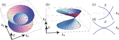
Figure 6: Bird’s eye’s view of (a) the Fermi loop, and (b) the point-nodal semimetal with a Dirac cone. Band structure of the semimetal along (a) the $k_{x}$ axis and (b) the $k_{y}$ axis. Energy spectrum is linear at the Dirac point. We have set $k_{z}=0$.

We have systematically constructed a wide class of the 3D honeycomb lattices indexed by $[\alpha_{1}\alpha_{2}\cdots\alpha_{N}]$. All of them are loop-nodal semimetals. Perfect flat bands will lead to the flat band ferromagnetism when the Coulomb interaction is included. With the SOI, they become strong topological insulators. It is intriguing that, with an additional AF order, point-nodal semimetals with Dirac cones are generated in the 3D space. Various 3D honeycomb lattices will be realized in the Li₂IrO₃ system since the building block of the 3D honeycomb lattice is naturally realized by the octahedron of the Ir networkModic . Our results will open a new physics of the honeycomb system in the three dimensions.

The authors is very much grateful to N. Nagaosa for many helpful discussions on the subject. This work was supported in part by Grants-in-Aid for MEXT KAKENHI grant number 25400317 and 15H05854.

References

- (1) D.J. Klein, Chem. Phys. Lett. 217, 261 (1994)
- (2) K. Nakada, M. Fujita, G. Dresselhaus and M. S. Dresselhaus, Phys. Rev. B, 54, 17954 (1996).
- (3) M. Ezawa, Phys. Rev. B, 73, 045432 (2006)
- (4) B. Wunsch, F. Guinea and F. Sols, New J. Phys. 10, 103027 (2008)
- (5) V. M. Pereira, A. H. Castro Neto, and N. M. R. Peres Phys. Rev. B 80, 045401 (2009)
- (6) G. Montambaux, F. Piechon, J.-N. Fuchs, and M. O. Goerbig, Phys. Rev. B 80, 153412 (2009)
- (7) M. Ezawa, New J. Phys. 16, 115004 (2014)
- (8) T. Takayama, A. Kato, R. Dinnebier, J. Nuss, H. Kono, L.?S.?I. Veiga, G. Fabbris, D. Haskel and H. Takagi, Phys. Rev. Lett. 114, 077202 (2015)
- (9) A. Biffin, et al, Phys. Rev. B. 90, 205116 (2014)
- (10) K. A. Modic, et.al.,Nat. Com. 5, 4203 (2014)
- (11) E.K.-H. Lee, S. Bhattacharjee, K. Hwang, H.-S. Kim, H. Jin and Y. B. Kim, Phys. Rev. B 89, 205132 (2014)
- (12) E. K.-H. Lee, R. Schaffer, S. Bhattacharjee and Y. B. Kim, Phys. Rev. B 89, 045117 (2014)
- (13) K. Mullen, B. Uchoa and D. T. Glatzhofer, Phys. Rev. Lett. 115, 026403 (2015)
- (14) J. Nasu, T. Kaji, K. Matsuura, M. Udagawa, and Y. Motome Phys. Rev. B 89, 115125 (2014)
- (15) I. Kimchi, J. G. Analytis, A. Vishwanath, Phys. Rev. B 90, 205126 (2014)
- (16) S. B. Lee, E. K.-H. Lee, A. Paramekanti and Y. B. Kim, Phys. Rev. B 89, 014424 (2014)
- (17) J. Nasu, M. Udagawa, Y. Motome, cond-mat/arXiv:1409.4865
- (18) M. Hermanns, K. O’Brien, and S. Trebst, Phys. Rev. Lett. 114, 157202 (2015)
- (19) I. Kimchi, R. Coldea and A. Vishwanath Phys. Rev. B 91, 245134 (2015)
- (20) M. Phillips and V. Aji, Phys. Rev. B, 90, 115111 (2014)
- (21) L. S. Xie, L. M. Schoop, E. M. Seibel, Q. D. Gibson, W. Xie, and R. J. Cava, APL Materials 3, 083602 (2015)
- (22) R. Yu, H. Weng,Z. Fang, X. Dai and X. Hu, cond-mat/arXiv:1504.04577
- (23) Y. Kim, B. J. Wieder, C. L. Kane, and A. M. Rappe, cond-mat/arXiv:1504.03807
- (24) M. Kohmoto, Y. Hasegawa, Phys. Rev. B 76, 205402 (2007)
- (25) C. L. Kane and E. J. Mele, Phys. Rev. Lett. 95, 226801 (2005)
- (26) L. Fu, C. L. Kane, and E. J. Mele, Phys. Rev. Lett. 98, 106803 (2007)