Schmidt-number benchmarks for continuous-variable quantum devices

Abstract

We present quantum fidelity benchmarks for continuous-variable (CV) quantum devices to outperform quantum channels which can transmit at most $k$-dimensional coherences for positive integers $k$. We determine an upper bound of an average fidelity over Gaussian distributed coherent states for quantum channels whose Schmidt class is $k$. This settles fundamental fidelity steps where the known classical limit and quantum limit correspond to the two endpoints of $k=1$ and $k=\infty$, respectively. It turns out that the average fidelity is useful to verify to what extent an experimental CV gate can transmit a high dimensional coherence. The result is further extended to be applicable to general quantum operations or stochastic quantum channels. While the fidelity is often associated with heterodyne measurements in quantum optics, we can also obtain similar criteria based on quadrature deviations determined via homodyne measurements.

I Introduction

It is a fundamental question how to generate and characterize higher dimensional entanglement on quantum systems Horodecki et al. (2009); Pan et al. (2012). A central tool to identify higher dimensional entanglement is the Schmidt number Terhal and Horodecki (2000). It is a convex roof extension of the Schmidt rank for pure bipartite quantum states, i.e., the rank of marginal density operators. A quantum state of a Schmidt-class $k$ implies the state can be expressed as a mixture of pure states whose Schmidt rank is at most $k$ for $k=1,2,3,\cdots$. On the level of quantum channels, the Schmidt-class $k$ implies that there exists a Kraus representation in which the maximum rank of Kraus operators is at most $k$ Huang (2006); Chruściński and Kossakowski (2006); Namiki (2013). A channel of Schmidt-class $k$ is also referred to as $k$-partially entanglement breaking ($k$-PEB) since it represents an important class of completely positive (CP) maps called entanglement breaking in the case of $k=1$ Horodecki et al. (2003); Holevo (2008). The notion of the Schmidt number tells us a precise meaning of the dimensionality in quantum object, and enables us to demonstrate multi-level coherences of quantum gates Namiki and Tokunaga (2012a) as well as to verify higher order entanglement in practical conditions Sanpera et al. (2001); Tokunaga et al. (2006, 2008); Inoue et al. (2009); Li et al. (2010); Sperling and Vogel (2011); Namiki and Tokunaga (2012b); Shahandeh et al. (2013); Gutiérrez-Esparza et al. (2014).

Quantum continuous-variable (CV) systems play a central role in quantum optics and experimental quantum information science Braunstein and van Loock (2005); Hammerer et al. (2010); Weedbrook et al. (2012). They are described by a set of bosonic field operators and capable of simulating any finite dimensional quantum information process in principle. However, their versatility could be limited due to various imperfections in experiments, and is not necessarily accessible in the original form of the theoretical model. Hence, it is natural to ask to what extent a given CV system is capable of simulating a higher dimensional quantum information process in practice. Notably, a verification scheme of higher dimensional entanglement of CV quantum states has been proposed Sperling and Vogel (2011); Shahandeh et al. (2013). However, it has little been studied how to verify higher dimensional gate coherences in CV quantum gates.

A practical measure to show a basic performance of CV gates Furusawa et al. (1998); Julsgaard et al. (2004); Lobino et al. (2009) is an average fidelity over an input ensemble of Gaussian distributed coherent states  Braunstein et al. (2000); Hammerer et al. (2005); Namiki et al. (2008); Takano et al. (2008). As an ultimate limitation of gate performance, the quantum limit fidelity was determined in Refs. Namiki (2011a); Chiribella and Xie (2013). On the other hand, the entanglement-breaking limit fidelity, which is normally referred to as the classical limit fidelity, was determined in Ref. Hammerer et al. (2005); Namiki et al. (2008); Namiki (2011b); Chiribella and Xie (2013); Yang et al. (2014); Namiki , and established a practical quantum benchmark for CV gates. Similarly to other quantum benchmarks Fuchs and Sasaki (2003); Namiki (2008); Häseler et al. (2008); Häseler and Lütkenhaus (2009); Owari et al. (2008); Namiki and Azuma (2015), the fidelity-based benchmark enables us to eliminate the possibility that the process is described by entanglement-breaking maps when the experimental fidelity is higher than the classical limit. Therefore, it can ensure the existence of the coherence in the lowest order of $k=2$, but could not provide evidence of substantially higher order coherences expected in CV gates.

Typically, we consider a higher fidelity implies a better gate performance, and it is likely that a higher fidelity suggests a higher Schmidt number and a higher order coherence. Therefore, an essential question is how high the fidelity need to be in order to outperform a wider class of lower dimensional processes which belong to the Schmidt class of a given Schmidt number $k$. Although the known Schmidt-number benchmarks Namiki and Tokunaga (2012a); Namiki could be usable in general, it is crucial to observe the gate performance using more accessible quantum optical measurements Namiki (2015). There are other possibilities to assess the gate coherence quantitatively by using different measures of entanglement Killoran and Lütkenhaus (2011); Killoran et al. (2012); Khan et al. (2013); Namiki (2015).

In this paper, we present Schmidt-number benchmarks for CV quantum devices based on an average fidelity over Gaussian distributed coherent states. We show an upper bound of the average fidelity achieved by $k$-PEB channels for any given positive integer $k$. It gives general fidelity steps that reproduce the classical limit and quantum limit for $k=1$ and $k=\infty$, respectively. Surpassing the $k$-th limit assesses the existence of $(k+1)$-dimension coherences on quantum channels and operations. We also provide a simple conjectural form of the tight $k$-th limit. This conjectured bound is partly achieved by a quantum channel with Schmidt-class $k$ and fully achievable by a probabilistic gate with Schmidt-class $k$, for every $k$. Furthermore, the fidelity bound is utilized to provide a different form for Schmidt-number benchmarks testable by using homodyne measurements.

The remainder of this paper is organized as follows. In Sec. II, we define the Schmidt-class-$k$ limit of the average fidelity for Gaussian distributed coherent states, and show how to find an upper bound. In Sec. III, we extend the resultant fidelity-based benchmarks for probabilistic quantum channels. In Sec. IV, we show a lower bound of an average quantum noise of canonical quadrature variables to outperform $k$-PEB operations as well as $k$-PEB channels. In Sec. V, we conclude this paper with remarks.

II Schmidt-class-$k$ fidelity limits for quantum channels

II.1 Ansatz

We consider transmission of coherent states $\left|\alpha\right\rangle:=D(\alpha)\left|0\right\rangle=e^{-|\alpha|^{2}/2}\sum_{n=0}^{\infty}\alpha^{n}\left|n\right\rangle/\sqrt{n!}$ through a quantum channel $\mathcal{E}$. Let us consider a transformation task on coherent states $\{|\alpha\rangle\}\to\{\left|\sqrt{\eta}\alpha\right\rangle\}$ with $\eta>0$, and define the average fidelity for Gaussian distributed coherent states as Braunstein et al. (2000); Hammerer et al. (2005); Namiki et al. (2008)

$$F_{\eta,\lambda}(\mathcal{E}):=\int p_{\lambda}(\alpha)\left\langle\sqrt{\eta}\alpha\right|\mathcal{E}\left(|\alpha\rangle\langle\alpha|\right)\left|\sqrt{\eta}\alpha\right\rangle d^{2}\alpha,$$ (1)

where $p_{\lambda}(\alpha)=\frac{\lambda}{\pi}\exp(-\lambda|\alpha|^{2})$ with $\lambda>0$. We define the Schmidt-class-$k$ fidelity limit of quantum channels by

$$F^{(k)}(\eta,\lambda):= \max_{\mathcal{E}\in\mathcal{O}_{k}}F_{\eta,\lambda}(\mathcal{E}),$$ (2)

where $\mathcal{O}_{k}$ is the set of $k$-PEB channels Huang (2006); Chruściński and Kossakowski (2006); Namiki (2013). This set can be defined in terms of Kraus operators $\sum_{i}K_{i}^{\dagger}K_{i}=\openone$ as

$$\mathcal{O}_{k}=\left\{\mathcal{E}\!\ \Big{|}\ \!\mathcal{E}(\rho)=\sum_{i}K_{i}\rho K_{i}^{\dagger}\wedge\forall i,\ \textrm{rank}(K_{i})\leq k\right\}.$$ (3)

Note that $\mathcal{O}_{1}$ represents the set of entanglement-breaking channels and $F^{(1)}$ corresponds to the classical limit fidelity Hammerer et al. (2005); Namiki et al. (2008). Note also that $\mathcal{O}_{\infty}$ forms the set of whole trace-preserving CP maps and $F^{(\infty)}$ corresponds to the quantum limit fidelity Namiki (2011a). Therefore, $F^{(k)}$ of Eq. (2) presents unified fidelity steps which include the classical limit and quantum limit as the two endpoints, $k=1$ and $k=\infty$. Our main goal is to find a non-trivial upper bound of $F^{(k)}$ for every integer $k\in[2,\infty)$.

Note that there is a general definition of PEB channels for CV systems Shirokov (2013). How to incorporate this general definition into our approach is beyond the scope of this paper.

II.2 Fidelity bounds

In order to find an upper bound of the fidelity $F^{(k)}$, we introduce a pair of two-mode states Namiki (2011b, a) as

$$\rho_{\mathcal{E}}:= \mathcal{E}\otimes I\left(\left|\psi_{\xi}\right\rangle\!\left\langle\psi_{\xi}\right|\right),$$ (4)

$$M:= \int p_{s}(\alpha)\left|\alpha\right\rangle\!\left\langle\alpha\right|\otimes\left|\kappa\alpha^{*}\right\rangle\!\left\langle\kappa\alpha^{*}\right|d^{2}\alpha,$$ (5)

where $I$ denotes the identity process, $\left|\psi_{\xi}\right\rangle=\sqrt{1-\xi^{2}}\sum_{n=0}^{\infty}\xi^{n}\left|n\right\rangle\left|n\right\rangle$ is a two-mode squeezed state with $\xi\in(0,1)$, and we assume $s,\kappa>0$. Using the relation $\langle\alpha|\psi_{\xi}\rangle=\sqrt{1-\xi^{2}}e^{-(1-\xi^{2})|\alpha|^{2}/2}\left|\xi\alpha^{*}\right\rangle$ we can find a state-based representation of the fidelity in Eq. (1) as

$$F_{1/N,\tau/N}(\mathcal{E}) =\frac{s+(1-\xi^{2})\kappa^{2}}{s(1-\xi^{2})}{\textrm{Tr}}(\rho_{\mathcal{E}}M),$$ (6)

where the parameters $(N,\tau)$ in the fidelity function are determined by

$$\tau =s+(1-\xi^{2})\kappa^{2},\ N=\kappa^{2}\xi^{2}.$$ (7)

From Eqs. (2) and (6) we have

$$F^{(k)}(1/N,\tau/N) =\frac{s+(1-\xi^{2})\kappa^{2}}{s(1-\xi^{2})}\max_{\mathcal{E}\in\mathcal{O}_{k}}{\textrm{Tr}}(\rho_{\mathcal{E}}M).$$ (8)

If $\mathcal{E}$ is a $k$-PEB channel, $\rho_{\mathcal{E}}=\mathcal{E}\otimes I\left(\left|\psi_{\xi}\right\rangle\!\left\langle\psi_{\xi}\right|\right)$ is a state of Schmidt-class $k$. This implies that the term $\max_{\mathcal{E}\in\mathcal{O}_{k}}{\textrm{Tr}}(\rho_{\mathcal{E}}M)$ in Eq. (8) can be upper bounded as

$$\max_{\mathcal{E}\in\mathcal{O}_{k}}{\textrm{Tr}}(\rho_{\mathcal{E}}M)\leq \max_{\phi\in S_{k}}\left\langle\phi\right|M\left|\phi\right\rangle,$$ (9)

where $S_{k}$ denotes the set of pure states whose Schmidt rank is $k$ or less than $k$.

To proceed, we use the fact that $M$ is invariant under the collective rotation $e^{i\theta(\hat{n}_{b}-\hat{n}_{a})}$. Here, $\hat{n}_{a}\ (\hat{n}_{b}$) stands for the number operator of the first (second) mode. This implies that $M$ can be decomposed into the direct-sum form associated with the eigenspaces of the relative photon-number operator $\hat{n}_{b}-\hat{n}_{a}=\sum_{J}J\openone^{(J)}$ as

$$M=\sum_{J=-\infty}^{\infty}\openone^{(J)}M\openone^{(J)}=:\bigoplus_{J=-\infty}^{\infty}M^{(J)},$$ (10)

where the identities of the orthogonal subspaces can be written as $\openone^{(J)}=\sum_{n=0}^{\infty}\left|e_{n}^{(J)}\right\rangle\!\left\langle e_{n}^{(J)}\right|$ with $\left|e_{n}^{(J)}\right\rangle:=\left|n\right\rangle\left|n+J\right\rangle$ for $J\geq 0$ and $\left|e_{n}^{(J)}\right\rangle:=\left|n-J\right\rangle\left|n\right\rangle$ for $J<0$. As a consequence, an explicit form for $M^{(J)}$ is given by

$$M^{(J)}=\frac{s}{(1+s+\kappa^{2})}\sum_{n,m=0}^{\infty}\gamma_{n,m}^{(J)}\left|e_{n}^{(J)}\right\rangle\!\left\langle e_{m}^{(J)}\right|,$$ (11)

where we define

$$\gamma_{n,m}^{(J)}:= \frac{(n+m+|J|)!\cdot\kappa^{J}x^{n+m+|J|}}{\sqrt{n!m!(n+|J|)!(m+|J|)!}}$$ (12)

and

$$x=\frac{\kappa}{1+s+\kappa^{2}}\leq\frac{1}{2}.$$ (13)

From this decomposition and theorem 2 of Ref. Sperling and Vogel (2011), we can see that a Schmidt-number $k$ vector $\left|\phi\right\rangle=\sum a_{n}|e_{n}^{(J)}\rangle$ in support of $M^{(J)}$ solves the Schmidt-number-eigenvalue problem of $M$. This implies that an upper bound is given by comparing the maximum on each subspace:

$$\max_{\psi\in S_{k}}\left\langle\phi\right|M\left|\phi\right\rangle =\max_{J}\max_{\phi\in S_{k}}{\textrm{Tr}}(M^{(J)}\left|\phi\right\rangle\!\left\langle\phi\right|).$$ (14)

Now, concatenating Eqs. (8, 9, 11, 14) and taking the limit $s\to 0$ with the help of Eq. (7) we obtain

$$F^{(k)}(1/N,\tau/N)\leq\frac{N+\tau}{1+N+\tau}\max_{J}\max_{\phi\in S_{k}}\left\langle\phi\right|A^{(J)}\left|\phi\right\rangle,$$ (15)

where

$$A^{(J)}:=\sum_{n,m=0}^{\infty}\gamma_{n,m}^{(J)}\left|e_{n}^{(J)}\right\rangle\!\left\langle e_{m}^{(J)}\right|$$ (16)

and $\gamma^{(J)}$ is given by Eq. (12) with $\kappa=\sqrt{N+\tau}$ and $x=\sqrt{N+\tau}/(1+N+\tau)$. Note that, for $\kappa\geq 1$ ($\kappa<1$), the optimization over $J\geq 0$ $(J\leq 0)$ is sufficient due to the relation $\kappa^{-J}\gamma_{n,m}^{(J)}=\kappa^{J}\gamma_{n,m}^{(-J)}$ or equivalently $\kappa^{-J}A^{(J)}=\kappa^{J}A^{(-J)}$.

Since $A^{(J)}$ of Eq. (16) is essentially the same form as $L$ of Eq. (63) in Ref. Sperling and Vogel (2011), we can evaluate $\max_{\phi\in S_{k}}\left\langle\phi\right|A^{(J)}\left|\phi\right\rangle$ by the maximal eigenvalue of all $k\times k$-principal submatrices of $A^{(J)}$. This enables us to determine an upper bound of $F^{(k)}$ as follows. Let us write a $k\times k$ principal submatrix of $A^{(J)}$ by

$$A^{(J)}_{\vec{n}}:=\sum_{n,m\in\vec{n}}\left|e_{n}^{(J)}\right\rangle\!\left\langle e_{n}^{(J)}\right|A^{(J)}\left|e_{m}^{(J)}\right\rangle\!\left\langle e_{m}^{(J)}\right|$$ (17)

where $\vec{n}={\{n_{1},n_{2},\cdots,n_{k}\}}$ is a set of non-negative integers in increasing order, $n_{l}<n_{l^{\prime}}$ with $l<l^{\prime}$, and the number of elements is denoted by $|\vec{n}|=k$. Then, we can formally express the fidelity bound as

$$F^{(k)}(1/N,\tau/N)\leq\frac{N+\tau}{1+N+\tau}\max_{J}\max_{|\vec{n}|=k}\|A^{(J)}_{\vec{n}}\|=:U_{k},$$ (18)

where $\|\cdot\|$ denotes the maximum eigenvalue.

The right-hand-side formula of Eq. (18) still involves optimizations over the integer $J$ and the choice of the $k$-tuple $\vec{n}$. Fortunately, we can find the maximum by checking a finite set of finite-size matrices once the parameters $(k,N,\tau)$ are fixed. This is because $\{A^{(J)}\}_{J}$ is essentially equivalent to the density matrix for the Gaussian state $M$ in the number basis, and the contribution involving sufficiently large photon-number elements is negligible. A practical process to determine the maximum is given in Appendices. Eventually, we can find the maximum by filtering out the submatrices whose maximal eigenvalue is smaller than that of another submatrix. In Appendix A, the optimal set $\vec{n}$ is identified for a couple of smaller $k$ in the case of $J=0$. Appendix B generalizes the approach presented in Appendix A, and gives a systematic process to determine the maximum over general $(J,\vec{n})$ for any given integer $k\in[1,\infty)$.

II.3 Numerical results and application

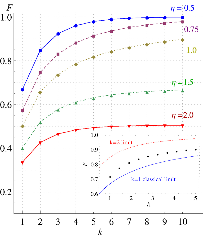
Figure 1: Our upper bound of the Schmidt-class-$k$ fidelity $F^{(k)}(\eta,\lambda)$ [$U_{k}$ of Eq. (18)] for $\lambda=0.01$ and $\eta\in\{0.5,0.75,1.0,1.5,2.0\}$. If an experimental fidelity $F_{\eta,\lambda}(\mathcal{E})$ stays above the $k$-th bound, the experimental CV gate $\mathcal{E}$ cannot be described by a $k$-PEB channel. This certificates an existence of the $(k+1)$-th coherence in the CV gate $\mathcal{E}$. The classical limit fidelity of the fundamental quantum benchmark corresponds to the bound of $k=1$. In the inset, the classical limit fidelity ($k=1$) and the fidelity bound for $k=2$ due to right-hand side of Eq. (20) are shown as a function of the Gaussian inverse width $\lambda$ for the case of unit-gain condition $\eta=1$. The dots represent the average fidelity $F_{1,\lambda}$ given in Fig. 5 of Ref. Lobino et al. (2009). This experimental fidelity is not high enough to give evidence to outperform an arbitrary qubit gate with regard to our criterion.

Based on the method described in Appendix B, we can numerically determine the upper bound of $F^{(k)}$ in Eq. (18). Figure 1 shows our bound of $F^{(k)}(\eta,\lambda)$ for $k=\{1,2,\cdots,10\}$ and $\eta\in\{0.5,0.75,1.0,1.5,2.0\}$ with $\lambda=0.01$. For each pair of the parameters $\{\eta,\lambda\}$, surpassing the bound of $k$ implies that the channel $\mathcal{E}$ outperforms $k$-PEB channels of Eq. (3), and is capable of transmitting entanglement of Schmidt-rank $k+1$. It certifies the quantum coherence unachievable by any teleportation-based quantum gate employing entanglement of Schmidt-class $k$ Namiki (2013). The fidelity steps agree with our intuition that a higher fidelity means an existence of stronger entanglement in terms of the Schmidt number, and would be widely useful to evaluate the performance of CV quantum gates.

Lobino et al., Lobino et al. (2009) showed an experimental average fidelity as a function of $\lambda$ for unit gain $\eta=1$. In the inset of Fig. 1 we find that the experimental fidelities are located in between the lines $k=1$ and $k=2$, and not high enough to demonstrate $k=3$ or higher dimensional coherences. This suggests that CV experiments are rather behind demonstrating genuinely higher dimensional coherences compared with experiments for multi-qubit channels Namiki and Tokunaga (2012a). It might be worth noting that the current fidelity record 83% for an experiment of a unit-gain teleportation protocol is a fidelity for an input of the vacuum state Yukawa et al. (2008); Pirandola et al. (2015). This corresponds to the case of $\lambda=\infty$ in our footing, and is useless for a verification of the multi-level coherence.

II.4 Conjecture and attainability

From the numerical results, it has been observed that the largest eigenvalue is given by the first $k\times k$ submatrix $A^{(0)}_{\{0,1,2,\cdots,k-1\}}$, namely, $\max_{J}\max_{|\vec{n}|=k}\|A^{(J)}_{\vec{n}}\|=\|A^{(0)}_{\{0,1,2,\cdots,k-1\}}\|$. Moreover, we can reproduce the expressions of the classical limit Namiki et al. (2008); Namiki (2011b) and the quantum limit Namiki (2011a) from the subspace of $J=0$ for $k=1$ and $k=\infty$. To be concrete, it holds that

$$F^{(1)}(1/N,\tau/N) = \frac{N+\tau}{1+N+\tau}\|A^{(0)}_{\{0\}}\|=\frac{N+\tau}{1+N+\tau},$$

$$F^{(\infty)}(1/N,\tau/N) \leq \frac{N+\tau}{1+N+\tau}\|A^{(0)}\|$$ (19)

$$= \frac{(N+\tau+1)-|N+\tau-1|}{2}.$$

We thus make a conjecture that the general limit is given by a significantly simple form:

$$F^{(k)}(1/N,\tau/N)\leq\frac{N+\tau}{1+N+\tau}\|A^{(0)}_{\{0,1,2,\cdots,k-1\}}\|.$$ (20)

Regarding the tightness of this conjectured bound, we present a $k$-PEB channel which saturates the inequality of Eq. (20) when $\tau\to 0$. Let us define a $k$-PEB channel $\mathcal{E}^{(k)}(\rho)=\int d^{2}\alpha K_{\alpha}^{(k)}\rho{(K_{\alpha}^{(k)})}^{\dagger}$ with Kraus operators of rank $k$ or less-than $k$

$$K_{\alpha}^{(k)}:=\frac{1}{\sqrt{\pi}}D\left(\frac{\sqrt{\eta}\alpha}{1+\lambda}\right)\left(\sum_{n=0}^{k-1}a_{n}^{(k)}\left|n\right\rangle\!\left\langle n\right|\right)D^{\dagger}(\alpha).$$ (21)

It fulfills $\int d^{2}\alpha{(K_{\alpha}^{(k)})}^{\dagger}K_{\alpha}^{(k)}=\openone$ by imposing the condition $\sum_{n=0}^{k-1}a_{n}^{2}=1$ and gives a simple form of the fidelity

$$\lim_{\lambda\to 0}F_{\eta,\lambda}(\mathcal{E}^{(k)}) = \sum_{n,m=0}^{k-1}\frac{a_{n}a_{m}\sqrt{\eta}^{n+m}}{n!m!}\left(\frac{-\partial}{\partial\eta}\right)^{n+m}\!\!\frac{1}{1+\eta}$$ (22)

$$= \frac{1}{1+\eta}\sum_{n,m=0}^{k-1}a_{n}\gamma_{n,m}^{(0)}a_{m}=:f^{(k)},$$

where $\gamma_{n,m}^{(0)}$ is given by Eq. (12) with $x=\sqrt{\eta}/(1+\eta)$. This implies $\max_{\{a_{n}\}}f^{(k)}=(1-\eta)^{-1}\|A_{\{0,1,\cdots,k-1\}}^{(0)}\|$, and $\mathcal{E}^{(k)}$ achieves the conjectured bound of Eq. (20) for $\tau=0$. It was shown that $\mathcal{E}^{(1)}$ achieves the classical limit in Ref. Namiki et al. (2008). For $k=2$ and $k=3$, we have observed numerically that $\mathcal{E}^{(k)}$ could not achieve the limit when $\tau>0$. Interestingly, we can generally show that the conjectured fidelity bound in Eq. (20) is achievable by a probabilistic quantum gate of Schmidt-class $k$ for every $k$ (See Sec III.2).

III Extension for general quantum operations

Our benchmarks can be extended for general quantum operations, namely, trace-non-increasing class of CP maps (See Ref. Namiki for a general framework). In Sec. III.1 we show that the bound $U_{k}$ of Eq. (18) holds for CP maps of Schmidt-class $k$ with a modified form of the fidelity. Notably, the bound $U_{k}$ is tight when general quantum operations are taken into account. An interesting example of trace-decreasing CP maps for CV states is the so-called noiseless linear amplifier or probabilistic amplifiers Ralph and Lund ; Chrzanowski et al. (2014); Xiang et al. (2010); Neergaard-Nielsen et al. (2013); Namiki (2015); Chiribella and Xie (2013). In Sec. III.2, we prove that such a stochastic quantum channel achieves the conjectured bound of Eq. (20).

III.1 Fidelity bounds for CP maps

Suppose that $\mathcal{E}$ is a quantum operation, namely, a trace-non-increasing CP map. We may modify the definition of the fidelity in Eq. (1) as Chiribella and Xie (2013)

$$F_{\eta,\lambda}(\mathcal{E}):=P_{s}^{-1}\int p_{\lambda}(\alpha)\left\langle\sqrt{\eta}\alpha\right|\mathcal{E}\left(|\alpha\rangle\langle\alpha|\right)\left|\sqrt{\eta}\alpha\right\rangle d^{2}\alpha,$$ (23)

where $p_{\lambda}(\alpha)=\frac{\lambda}{\pi}\exp(-\lambda|\alpha|^{2})$ with $\lambda>0$, and $P_{s}:={{\textrm{Tr}}\int p_{\lambda}(\alpha)\mathcal{E}(\left|\alpha\right\rangle\!\left\langle\alpha\right|)d^{2}\alpha}$ is the probability that $\mathcal{E}$ gives an output state for the ensemble $\{p_{\lambda}(\alpha),\left|\alpha\right\rangle\!\left\langle\alpha\right|\}$. Note that Eq. (23) reduces to Eq. (1) for the trace-preserving case, i.e., for quantum channels. In fact, ${\textrm{Tr}}[\mathcal{E}(\left|\alpha\right\rangle\!\left\langle\alpha\right|)]=1$ for all $\alpha\in\mathbb{C}$ implies $P_{s}=1$.

Similarly to Eq. (2), let us define the Schmidt-class-$k$ fidelity limit with the renormalized fidelity in Eq. (23) as

$$F^{(k)}(\eta,\lambda) := \max_{\mathcal{E}\in\mathcal{O}_{k}}F_{\eta,\lambda}(\mathcal{E}),$$ (24)

where $\mathcal{O}_{k}$ denotes the set of $k$-PEB maps described by $\mathcal{E}(\rho)=\sum_{i}K_{i}\rho K_{i}^{\dagger}$. Here, operators $\{K_{i}\}$ have rank $k$ or less than $k$ (We do not impose trace-preserving condition $\sum_{i}K_{i}^{\dagger}K_{i}=\openone$).

In order to show that the same fidelity bound $U_{k}$ in Eq. (18) holds for quantum operations Namiki , the key is to employ the normalized state:

$$\rho_{\mathcal{E}}: = \frac{\mathcal{E}\otimes I\left(\left|\psi_{\xi}\right\rangle\left\langle\psi_{\xi}\right|\right)}{{\textrm{Tr}}\left[\mathcal{E}\otimes I\left(\left|\psi_{\xi}\right\rangle\left\langle\psi_{\xi}\right|\right)\right]}.$$ (25)

By using this formula, instead of Eq. (4), the procedure in Sec. II.2 leads to the fidelity bound for general CP maps:

$$F^{(k)}(\eta,\lambda)\leq U_{k}(\eta,\lambda)=\frac{1+\lambda}{1+\eta+\lambda}\max_{J}\max_{|\vec{n}|=k}\|A^{(J)}_{\vec{n}}\|,$$ (26)

where $\|\cdot\|$ denotes the maximum eigenvalue and $A^{(J)}_{\vec{n}}$ is defined through Eqs. (12), (16), and (17) with

$$x=\frac{\sqrt{\eta(1+\lambda)}}{1+\eta+\lambda},\ \kappa=\sqrt{\frac{1+\lambda}{\eta}}.$$ (27)

Note that Eq. (26) is tight, namely, it holds that

$$F^{(k)}(\eta,\lambda)=U_{k}(\eta,\lambda).$$ (28)

This can be confirmed from the fact that $U_{k}$ is a solution of the Schmidt-number-eigenvalue problem Sperling and Vogel (2011) together with the property of $k$-PEB maps that $\rho_{\mathcal{E}}$ of Eq. (25) can be any pure state of Schmidt-number $k$. For quantum channels (trace-preserving CP maps), it remains open how to find tight limit except for the classical limit $k=1$ Namiki et al. (2008) and quantum limit $k=\infty$ Namiki (2011a); Chiribella and Xie (2013).

By comparing an experimentally observed fidelity and our upper bound of the $k$-th fidelity limit $F^{(k)}$, one can verify a genuine multi-dimensional coherence for general quantum operations as well as for quantum channels. To be concrete, we can eliminate the possibility that the physical process $\mathcal{E}$ is described as a $k$-PEB map if it holds that $F_{\eta,\lambda}(\mathcal{E})>U_{k}(\eta,\lambda)$. This establishes an infinite sequence of quantitative quantum benchmarks for general single-mode physical processes with respect to the Schmidt number, $k$. The fidelity steps $U_{k}(\eta,\lambda)$ would give distinctive milestones to assess the closeness between an experimental amplifier and an ideal quantum limited amplification process Chiribella and Xie (2013); Namiki (2015) by simultaneously observing the Schmidt number and the fidelity.

III.2 Proof of attainability of the conjectured bound

In Sec. II.4, we have conjectured that the simple form in Eq. (20) gives a tighter bound. Here, we will show that a probabilistic quantum channel of Schmidt-class $k$ achieves the conjectured bound:

$$F^{(k)}(\eta,\lambda)\leq\frac{1+\lambda}{1+\eta+\lambda}\|A^{(0)}_{\{0,1,2,\cdots,k-1\}}\|.$$ (29)

Proof.— Let us consider the following filtering operator

$$Q_{k}=\sqrt{\mathcal{N}}\sum_{n=0}^{k-1}a_{n}g^{n}\left|n\right\rangle\!\left\langle n\right|$$ (30)

where $(\mathcal{N},g$) is a pair of positive constants and we assume $\sum_{n=0}^{k-1}|a_{n}|^{2}=1$. We can readily calculate its action onto coherent states as

$$Q_{k}\left|\alpha\right\rangle=\sqrt{\mathcal{N}}e^{-|\alpha|^{2}/2}\sum_{n=0}^{k-1}\frac{a_{n}(g\alpha)^{n}}{\sqrt{n!}}\left|n\right\rangle.$$ (31)

Evidently, $Q_{k}$ is rank $k$ or less than $k$. This implies that the probabilistic quantum gate $\mathcal{E}(\rho)=Q_{k}\rho Q_{k}^{\dagger}$ belongs to Schmidt-class $k$. From these expressions we have

$$\int p_{\lambda}(\alpha)\left\langle\sqrt{\eta}\alpha\right|\mathcal{E}\left(|\alpha\rangle\langle\alpha|\right)\left|\sqrt{\eta}\alpha\right\rangle d^{2}\alpha$$

$$= \mathcal{N}\lambda\sum_{n,m=0}^{k-1}\frac{(n+m)!}{n!m!}\frac{(\sqrt{\eta}g)^{m+m}a_{n}a_{m}^{*}}{(1+\eta+\lambda)^{n+m+1}}$$

$$= \frac{\mathcal{N}\lambda}{1+\eta+\lambda}\sum_{n,m=0}^{k-1}\gamma_{n,m}^{(0)}a_{n}a_{m}^{*},$$ (32)

where we use $\int p_{\lambda}(\alpha)e^{-(1+\eta)|\alpha|^{2}}|\alpha|^{2k}d^{2}\alpha=\lambda{k!}/{(1+\eta+\lambda)^{k+1}}$ for calculating the integration. Moreover, the final expression is obtained by substituting $g=\sqrt{1+\lambda}$ and using the definition of $\gamma_{n,m}^{(0)}$ in Eq. (12) where the parameter $x$ is given by Eq. (27). Note that, from the definition of the submatrix $A_{\vec{n}}^{(J)}$ given through Eqs. (12), (16), and (17), we can write

$$\max\left(\sum_{n,m=0}^{k-1}{\gamma_{n,m}^{(0)}a_{n}a_{m}^{*}}\right)=\|A_{\{0,1,2,\cdots,k-1\}}^{(0)}\|,$$ (33)

where the maximum is taken over $\sum_{n=0}^{k-1}|a_{n}|^{2}=1$.

On the other hand, the relation in Eq. (31) and the condition $g=\sqrt{1+\lambda}$ yield the following expression:

$$P_{s} ={{\textrm{Tr}}\int p_{\lambda}(\alpha)\mathcal{E}(\left|\alpha\right\rangle\!\left\langle\alpha\right|)d^{2}\alpha}$$

$$=\mathcal{N}\lambda\sum_{n=0}^{k-1}\frac{|a_{n}|^{2}g^{2n}}{(1+\lambda)^{n+1}}=\frac{\mathcal{N}\lambda}{1+\lambda}\sum_{n=0}^{k-1}|a_{n}|^{2}=\frac{\mathcal{N}\lambda}{1+\lambda}.$$ (34)

From Eqs. (23), (32), and (34) we obtain

$$F_{\eta,\lambda}(\mathcal{E})=\frac{1+\lambda}{1+\eta+\lambda}\sum_{n,m=0}^{k-1}\gamma_{n,m}^{(0)}a_{n}a_{m}^{*}.$$ (35)

Finally, optimizing the coefficient $\{a_{n}\}$ of the filter $Q_{k}$ as in Eq. (33) we can conclude that the right-hand side of Eq. (29) [Eq. (20)] is achievable by a probabilistic quantum gate of Schmidt-class $k$. $\blacksquare$

Note that the normalization factor $\mathcal{N}$ of $Q_{k}$ in Eq. (30) can be positive as long as $k$ is finite. This fact confirms the attainability with a finite success probability $P_{s}>0$. In the limit of $k\to\infty$, however, $\mathcal{N}$ could be zero so as to fulfill the physical condition $Q_{k}^{\dagger}Q_{k}\leq\openone$ (See Refs. Chiribella and Xie (2013); Namiki (2015)).

IV Schmidt-class-$k$ limitation on quantum noise of canonical variables

In this section, we present a Schmidt-class-$k$ limit on an average of Bayesian mean-square deviations for canonical variables. We introduce a basic relation between the fidelity and quantum noise in Sec. IV.1. Resultant Schmidt-number benchmarks are given in Sec. IV.2.

IV.1 Canonical quantum noise and fidelity

Let $\hat{x}$ and $\hat{p}$ be canonical quadrature variables with the canonical commutation relation $[\hat{x},\hat{p}]=i$. The field operator $\hat{a}$ is given as $\hat{a}=(\hat{x}+i\hat{p})/\sqrt{2}$, and satisfies the bosonic commutation relation, $[\hat{a},\hat{a}^{\dagger}]=1$. For notation convention we write the mean quadratures for coherent states as

$$x_{\alpha}:=\left\langle\alpha\right|\hat{x}\left|\alpha\right\rangle=\frac{\alpha+\alpha^{*}}{\sqrt{2}},\ p_{\alpha}:=\left\langle\alpha\right|\hat{p}\left|\alpha\right\rangle=\frac{\alpha-\alpha^{*}}{\sqrt{2}i}.$$ (36)

Let $\mathcal{E}$ be a quantum operation. We define the mean-square deviations for canonical quadratures Namiki et al. (2008); Namiki and Azuma (2015); Namiki (2015) as

$$\bar{V}_{z}:=P_{s}^{-1}{\textrm{Tr}}\left[\int p_{\lambda}(\alpha)(\hat{z}-\sqrt{\eta}z_{\alpha})^{2}\mathcal{E}(\left|\alpha\right\rangle\!\left\langle\alpha\right|)d^{2}\alpha\right],$$ (37)

where $z\in\{x,p\}$, $p_{\lambda}(\alpha):=\frac{\lambda}{\pi}\exp(-\lambda|\alpha|^{2})$, and $P_{s}:={{\textrm{Tr}}\int p_{\lambda}(\alpha)\mathcal{E}(\left|\alpha\right\rangle\!\left\langle\alpha\right|)d^{2}\alpha}$. With the help of the property of the displacement operator $D(\alpha)\hat{a}D^{\dagger}(\alpha)=\hat{a}-\alpha$ and the cyclic property of the trace, we can write

$$\bar{V}_{z}= P_{s}^{-1}{\textrm{Tr}}\left[\int p_{\lambda}(\alpha)D(\sqrt{\eta}\alpha)\hat{z}^{2}D^{\dagger}(\sqrt{\eta}\alpha)\mathcal{E}(\left|\alpha\right\rangle\!\left\langle\alpha\right|)d^{2}\alpha\right]$$

$$= P_{s}^{-1}{\textrm{Tr}}[\hat{z}^{2}\sigma],$$ (38)

where we defined

$$\sigma:= \int p_{\lambda}(\alpha)D^{\dagger}(\sqrt{\eta}\alpha)\mathcal{E}(\left|\alpha\right\rangle\!\left\langle\alpha\right|)D(\sqrt{\eta}\alpha)d^{2}\alpha.$$ (39)

Note that we can readily confirm the following relations:

$${\textrm{Tr}}[\sigma]= {\textrm{Tr}}\int p_{\lambda}(\alpha)\mathcal{E}(\left|\alpha\right\rangle\!\left\langle\alpha\right|)d^{2}\alpha=P_{s},$$

$$\left\langle 0\right|\sigma\left|0\right\rangle= \int p_{\lambda}(\alpha)\left\langle\sqrt{\eta}\alpha\right|\mathcal{E}(\left|\alpha\right\rangle\!\left\langle\alpha\right|)\left|\sqrt{\eta}\alpha\right\rangle d^{2}\alpha.$$ (40)

From Eq. (38) and the well-known expression for the harmonic oscillator, $\hat{x}^{2}+\hat{p}^{2}=2\hat{a}^{\dagger}\hat{a}+1$, the sum of the mean-square deviations can be expressed as

$$\bar{V}_{x}+\bar{V}_{p}= \frac{1}{P_{s}}(2{\textrm{Tr}}[\hat{a}^{\dagger}\hat{a}\sigma]+{\textrm{Tr}}[\sigma]).$$ (41)

On the other hand, we can show the following inequality for any positive semidefinite operator $\rho$:

$${\textrm{Tr}}[\hat{a}^{\dagger}\hat{a}\rho]= {\textrm{Tr}}\left(\sum_{n=1}^{\infty}n\left|n\right\rangle\!\left\langle n\right|\rho\right)$$

$$\geq {\textrm{Tr}}\left(\sum_{n=1}^{\infty}\left|n\right\rangle\!\left\langle n\right|\rho\right)={\textrm{Tr}}[\rho]-\left\langle 0\right|\rho\left|0\right\rangle.$$ (42)

Concatenating Eqs. (40), (41), and (42) with $\rho=\sigma$, we obtain the relation between the sum quantum noise and the average fidelity Namiki et al. (2008)

$$\bar{V}_{x}+\bar{V}_{p}-1\geq \frac{2}{P_{s}}({\textrm{Tr}}[\sigma]-\left\langle 0\right|\sigma\left|0\right\rangle)=2\left(1-F_{\eta,\lambda}\right),$$ (43)

where $F_{\eta,\lambda}$ is defined in Eq. (23). From Eq. (43), we can see that a smaller value of quantum noise ensures a higher fidelity. To be concrete, Eq. (43) implies that the fidelity is bounded from below by using the mean-square deviations

$$F_{\eta,\lambda}\geq \frac{3}{2}-\frac{\bar{V}_{x}+\bar{V}_{p}}{2}.$$ (44)

In particular, we can observe that $F=1$ if $V_{x}+V_{p}=1$.

IV.2 Schmidt-number benchmarks via quantum noise

Now, we can find a lower bound of the Schmidt number by using the sum of the mean-square deviations $V_{x}$ and $V_{p}$. We can show that $F_{\eta,\lambda}(\mathcal{E})>F^{(k)}(\eta,\lambda)$ holds if the following condition is satisfied

$$\bar{V}_{x}+\bar{V}_{p}-1<2(1-F^{(k)}(\eta,\lambda)).$$ (45)

Proof.— Suppose Eq. (45) holds. From Eqs. (43) and (45), we have

$$2\left(1-F_{\eta,\lambda}\right)\leq\bar{V}_{x}+\bar{V}_{p}-1<2(1-F^{(k)}(\eta,\lambda)).$$ (46)

Comparing the left-end and right-end expressions, we obtain $F_{\eta,\lambda}(\mathcal{E})>F^{(k)}(\eta,\lambda)$. Hence, Eq. (45) is a sufficient condition that $\mathcal{E}$ outperforms any $k$-PEB maps. $\blacksquare$

For a practical use, one can replace the term $F^{(k)}$ in Eq. (45) with the upper bound $U_{k}$ given in Eq. (18). We thus have the following quantum benchmark:

$$\bar{V}_{x}+\bar{V}_{p}-1<2(1-U_{k}(\eta,\lambda)).$$ (47)

This condition can be readily tested by plugging-in an experimentally observed value of $\bar{V}_{x}+\bar{V}_{p}$. Hence, one can verify that the Schmidt number of the process $\mathcal{E}$ is at least $k+1$ if the inequality of Eq. (47) is fulfilled.

Note that the condition of Eq. (45) is not tight when $k=1$ (See, Corollary 1 of Namiki and Azuma (2015)), and unlikely to be tight for other choice of $k\geq 2$. How to find a better link between the Schmidt class and the quadrature deviations for an improvement of our approach should be addressed elsewhere.

V Conclusion and remarks

In conclusion, we have presented Schmidt-number benchmarks for CV quantum devices using the average fidelity for Gaussian distributed coherent states. Our benchmarks give everlasting fidelity steps towards higher dimensional quantum-gate coherence, and successfully generalize the known classical and quantum limits by recasting them into the two endpoints of these steps. Our result refines the meaning of “high fidelity” for CV quantum gates, and the numerically determined fidelity steps would be useful to demonstrate genuinely higher dimensional coherence for experimental implementations. It is fundamentally important to show stronger evidence that CV systems have a potential superiority in dealing with higher dimensional quantum signals. In this respect, distinctive experimental progress could be regularly quantified and recorded based on the Schmidt class determined by the fidelity steps. We have also conjectured a simple formula for the fidelity bound. This bound is achievable by a probabilistic quantum gate of the corresponding Schmidt class. Furthermore, we have presented a lower bound of an average quantum noise to outperform $k$-PEB processes. This bound is directly related to homodyne measurements and could provide wider options for an experimental verification of higher dimensional coherences.

Although our results are readily available as a type of entanglement verification tools for experiments, there are several open possibilities to improve the fidelity bound and the bound for the canonical quantum noise. We remark the following three aspects for an outlook.

(i) Our fidelity bound $U_{k}$ is tight for quantum operations, yet we have not identified what operation can achieve this bound (In Sec. III.2 we have provided a concrete form of a probabilistic gate that achieves the conjectured bound. If the conjectured bound is proven equivalent to $U_{k}$, we can immediately settle this problem).

(ii) How to improve the fidelity bound $U_{k}$ for the case of quantum channels and how to identify the optimal $k$-PEB channel which maximizes the fidelity, for $k\in[2,\infty)$ remain open. In this regard, it has been known Chiribella and Xie (2013) that there is a gap between the quantum limit fidelities ($k\to\infty$) for probabilistic gates and deterministic gates, whereas there is no gap for the classical fidelity limits ($k=1$). An existence of the gap is crucial to demonstrate an advantage of probabilistic gates Namiki (2015).

(iii) Aside from the fidelity-based approach, exploring a feasible method based on the statistical moments of canonical variables would be important. As well as improving our bound for the sum of the mean-square deviations in Sec. IV.2, an interesting problem is to determine the trade-off relation between the mean-square deviations under the constraint of the Schmidt class. Hopefully, we could prove a general sequence of uncertainty relations for $V_{x}$ and $V_{p}$, which reproduces the uncertainty relation over Entanglement-breaking maps for $k=1$ Namiki and Azuma (2015) and approaches the amplification uncertainty relation Namiki (2015) in the limit $k\to\infty$.

Appendix A Rigorous result for the maximization in Eq. (18) for $J=0$

As a first step to estimate the maximization in Eq. (18), we consider the case of $J=0$. In the case of $J=0$ we can show that the exact maximum for $k=1$, 2, and 3 is given by

$$\max_{|\vec{n}|=k}\|A^{(0)}_{\vec{n}}\| = \|A^{(0)}_{\{0,1,2,\cdots,k-1\}}\|.$$ (48)

In order to verify this relation, we use the following two properties for $\gamma$ defined through Eqs. (12) and (13):
(i) $\gamma_{n+1,n-l+1}^{(0)}-\gamma_{n,n-l}^{(0)}\leq 0$ holds for $n\geq\frac{1}{2}(l+2)(l-l)$.
(ii) $\gamma_{n+1,m}^{(0)}-\gamma_{n,m}^{(0)}\leq 0$ holds for $m\leq n-1$.

First, Property (i) with $l=0$ implies that the diagonal elements are in decreasing order, namely, $\gamma_{0,0}^{(0)}\geq\gamma_{1,1}^{(0)}\geq\gamma_{2,2}^{(0)}\geq\cdots$. This proves Eq. (48) for $k=1$. Note that Property (i) with $l=1$ implies that the first off-diagonal elements are in decreasing order, namely, it holds that $\gamma_{0,1}^{(0)}\geq\gamma_{1,2}^{(0)}\geq\gamma_{2,3}^{(0)}\geq\cdots$. Similarly, Property (i) with $l=2$ implies that the second off-diagonal elements are in decreasing order, namely, it holds that $\gamma_{0,2}^{(0)}\geq\gamma_{1,3}^{(0)}\geq\gamma_{2,4}^{(0)}\geq\cdots$.

Next, to prove Eq. (48) for $k=2$ we show

$$\left(\begin{array}[]{cc}\gamma_{n,n}^{(0)}&\gamma_{n,n+1}^{(0)}\\ \gamma_{n+1,n}^{(0)}&\gamma_{n+1,n+1}^{(0)}\\ \end{array}\right)-\left(\begin{array}[]{cc}\gamma_{n+1,n+1}^{(0)}&\gamma_{n+1,n+2}^{(0)}\\ \gamma_{n+2,n+1}^{(0)}&\gamma_{n+2,n+2}^{(0)}\\ \end{array}\right)\geq 0,$$ (53)

$$\left(\begin{array}[]{cc}\gamma_{n,n}^{(0)}&\gamma_{n,n+1}^{(0)}\\ \gamma_{n+1,n}^{(0)}&\gamma_{n+1,n+1}^{(0)}\\ \end{array}\right)-\left(\begin{array}[]{cc}\gamma_{n,n}^{(0)}&\gamma_{n,n+n^{\prime}}^{(0)}\\ \gamma_{n+n^{\prime},n+n^{\prime}}^{(0)}&\gamma_{n+n^{\prime},n+n^{\prime}}^{(0)}\\ \end{array}\right)\geq 0,$$ (58)

(59)

where each inequality for matrices indicates all elements are non-negative. The first inequality suggests the decreasing order on shift in the diagonal direction associated with the schematics of Fig. 2(b); The second inequality suggests the decreasing order on spread in the vertical-and-horizontal direction associated with the schematics of Fig. 2(a). The first inequality of Eqs. (59) is proven from the decreasing order on the diagonal elements and the first off-diagonal elements. The second inequality of Eqs. (59) is proven by using the decreasing order on the diagonal elements and Property (ii). From the inequalities in Eqs. (59) we have $\|A^{(0)}_{\{n,n+1\}}\|\geq\|A^{(0)}_{\{n+1,n+2\}}\|$ and $\|A^{(0)}_{\{n,n+1\}}\|\geq\|A^{(0)}_{\{n,n+n^{\prime}\}}\|$ since $\|a\|\leq\|b\|$ holds for non-negative matrices $a$ and $b$ with $0\leq a\leq b$ (See, Corollary 8.1.19. of Horn and Johnson (2007)). Using these two relations recursively we can conclude Eq. (48) for $k=2$. Note that, from the order of the diagonal elements and Property (ii), we can generally obtain such a matrix inequality when the position of the final row and column is shifted as in Fig. 2c.

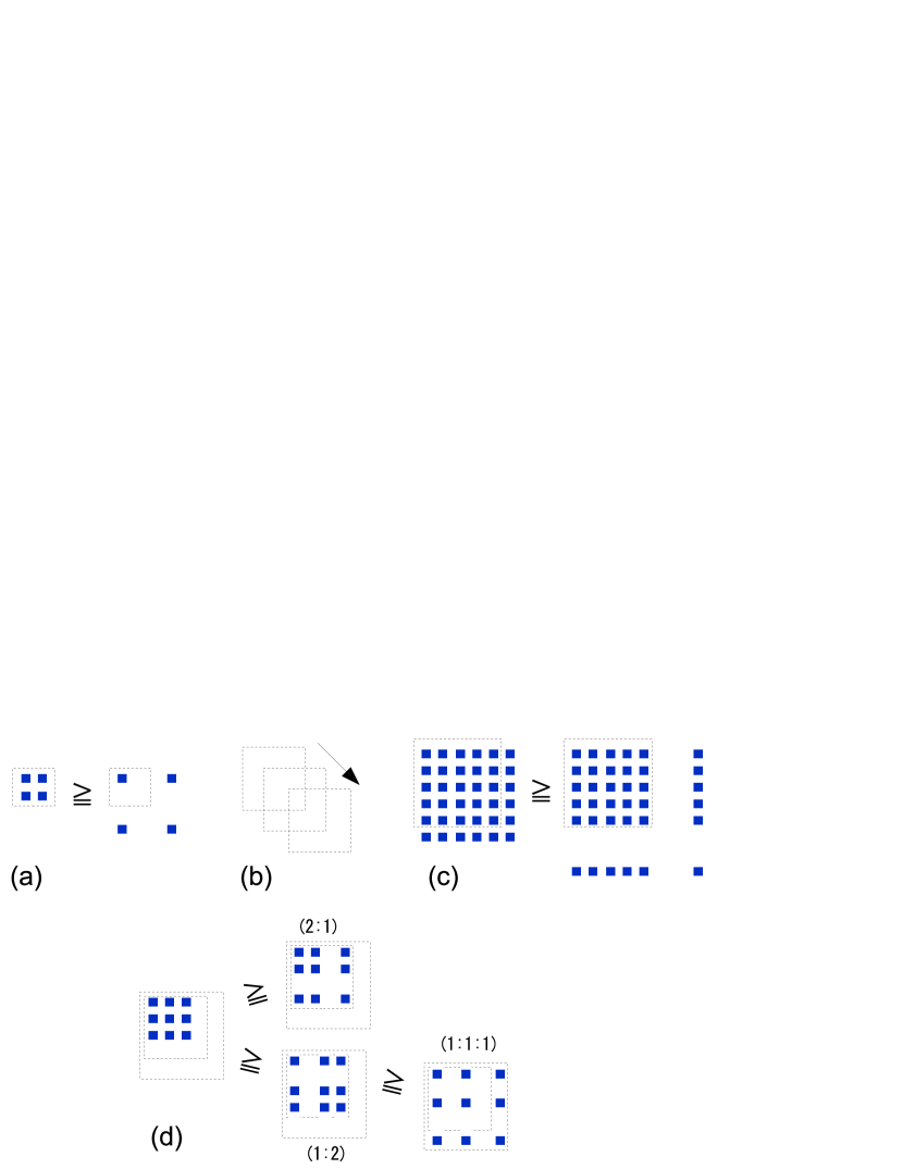
Figure 2: Orders of principal submatrices.

Finally, similar to this proof, we proceed to the proof of $k=3$ by comparing the corresponding submatrix elements associated with $\|A^{(0)}_{\{n,n+1,n+2\}}\|\geq\|A^{(0)}_{\{n+1,n+2,n+3\}}\|$ for the diagonal direction shift and $\|A^{(0)}_{\{n,n+1,n+2\}}\|\geq\|A^{(0)}_{\{n,n+n^{\prime},n+n^{\prime\prime}\}}\|$ for the spreading shift. For the diagonal shift of the $3\times 3$ matrix, the matrix inequality can be confirmed by the decreasing order on the diagonal elements, the first off-diagonal elements, and the second off-diagonal elements, coming from Property (i) with $l=0$, $1$, and $2$. For the spreading of the $3\times 3$ matrix, we have three possibilities to divide the elements (2:1), (2:1), and (1:1:1) as in Fig. 2(d). For the case of (2:1), the inequality can be proven by Property (ii) and the decreasing order on the diagonal elements. For the case of (1:2), the inequality can be proven by Property (ii) and the decreasing order on the diagonal shift of $2\times 2$ matrix. Then, the first inequality of Eq. (59) on $2\times 2$ matrix and the decreasing order on the diagonal elements again enable us to show the decreasing order on the spreading shift from (1:2) to (1:1:1). Therefore, we can conclude that the relation Eq. (48) holds for $k\in\{1,2.3\}$.

For $k=4$, we can show the inequality for the spreading shift $\|A^{(0)}_{\{n,n+1,n+2,n+3\}}\|\geq\|A^{(0)}_{\{n,n+n^{\prime},n+n^{\prime\prime},n+n^{\prime\prime\prime}\}}\|$ by using Property (ii) and the results of the $2\times 2$ and $3\times 3$ matrices above. Similarly, from Property (i) and the results of $k\leq 3$ above we have $\|A^{(0)}_{\{n,n+1,n+2,n+3\}}\|\geq\|A^{(0)}_{\{n+1,n+2,n+3,n+4\}}\|$ when $n\geq 2$. However, the matrix inequality for the diagonal shift could not hold for the first two submatrices, $A_{\{0,1,2,3\}}^{(0)}$ and $A_{\{1,2,3,4\}}^{(0)}$. Therefore, the maximum is obtained by comparing the first three cases of the matrices, i.e. $\max_{n\in\{0,1,2\}}\|A_{\{n,n+1,n+2,n+3\}}^{(0)}\|$. In this manner, we can eventually determine the maximum by comparing the maximum eigenvalues of a relatively small number of submatrices for a couples of small $k$. We present a general systematic approach to determine the maximum of Eq. (18) in the following section.

Appendix B General recipe to determine the maximum in Eq. (18)

In the previous section, we use the following two properties to make (matrix) inequalities on submatrices of $A^{(0)}$ defined through Eqs. (12) and (13):
(i) $\gamma_{n+1,n-l+1}^{(0)}-\gamma_{n,n-l}^{(0)}\leq 0$ holds for $n\geq\frac{1}{2}(l+2)(l-l)$.
(ii) $\gamma_{n+1,m}^{(0)}-\gamma_{n,m}^{(0)}\leq 0$ holds for $m\leq n-1$.

In this section, we develop this method and present a systematic approach to determine the maximum in Eq. (18). An essential fact to generate matrix inequalities is that $\|a\|\leq\|b\|$ holds for non-negative matrices $a$ and $b$ with $0\leq a\leq b$ (See, Corollary 8.1.19. of Horn and Johnson (2007)).

Let us note general properties of $A^{(J)}$. (a) $A^{(J)}$ is a non-negative matrix and symmetric, i.e., for any $n,m$, $\gamma_{n,m}^{(J)}\geq 0$ and $\gamma_{n,m}^{(J)}=\gamma_{m,n}^{(J)}$. (b) If $n\geq\frac{1}{2}(|J|-2)(|J|+1)$, we have $\gamma_{n+1,n+1}^{(J)}-\gamma_{n,n}^{(J)}\leq 0$. (c) The sequence of the diagonal elements $\{\gamma_{n,n}^{(J)}\}_{n}$ is at most single peaked and the largest element is located around $n\sim\frac{1}{2}(|J|^{2}-|J|-2)$. From these properties and the fact that eigenvalues of a positive semidefinite matrix are upper bounded by its trace, we can neglect the contribution from sufficiently large $n$ when we determine the maximum in Eq. (18), numerically.

B.1 Derivation of the properties (i) and (ii)

From Eqs. (12) and (13) we have

$$\gamma_{n+1,m+1}^{(J)}-\gamma_{n,m}^{(J)}\leq\gamma_{n,m}^{(J)}$$

$$\times\left(\frac{(n+m+|J|+2)(n+m+|J|+1)}{\sqrt{(n+1)(m+1)(n+|J|+1)(m+|J|+1)}}\frac{1}{4}-1\right).$$ (60)

Suppose that $m=n-l\leq n$. If we set $J=0$ we obtain Property (i). In our approach, a key observation is that any $l$-th off-diagonal element gradually gives a decreasing sequence. We define an integer $t_{l}$ to utilize this fact. The integer $t_{l}$ that fulfills $\gamma_{n+1,m+1}^{(J)}-\gamma_{n,m}^{(J)}\leq 0$ is summarized in Table 1 for $l\leq 10$. The row of $l=0$ shows all diagonal elements are in decreasing order for $|J|\leq 2$. The row of $l=1$ shows all first off-diagonal elements are in decreasing order for $|J|\leq 1$. Note that the values in Table 1 are determined by taking the worst case of $x=\frac{1}{2}$ (Better bounds would be obtained when a specific value of $x<\frac{1}{2}$ is given).

Suppose that $m\leq n-1$. From Eqs. (12) and (13) we have

$$\gamma_{n+1,m}^{(J)}-\gamma_{n,m}^{(J)} \leq \gamma_{n,m}^{(J)}\left(\frac{n+m+|J|+1}{\sqrt{(n+1)(n+|J|+1)}}\frac{1}{2}-1\right)$$

$$\leq \gamma_{n,m}^{(J)}\left(\frac{n+|J|/2}{\sqrt{(n+1)(n+|J|+1)}}-1\right).$$

This implies $\gamma_{n+1,m}^{(J)}-\gamma_{n,m}^{(J)}\leq 0$ for $|J|\leq 4$. For $|J|>4$, $\gamma_{n+1,m}^{(J)}-\gamma_{n,m}^{(J)}\leq 0$ is fulfilled when

$$n\geq(-4-4|J|+J^{2})/8=:u^{(J)}.$$ (62)

As a consequence, the case of $J=0$ gives Property (ii). Notably, the expressions derived here suggest that we can use modified versions of Properties (i) and (ii) for $J\neq 0$. Our main residual task is to make matrix inequalities systematically based on the general properties of $\{\gamma_{n,m}^{(J)}\}$.

Table 1: The integer $t_{l}^{(J)}$ in which $l$-th off-diagonal elements become decreasing order for $|J|\leq 4$. The superscript index “$(J)$” of $t_{l}^{(J)}$ is omitted through the text.

$l$	$J=0$	$|J|=1$	$|J|=2$	$|J|=3$	$|J|=4$
0	0	0	0	2	5
1	1	1	2	4	7
2	2	3	4	6	9
3	5	6	7	9	12
4	9	10	11	13	16
5	14	15	16	18	21
6	20	21	22	24	27
7	27	28	29	31	34
8	35	36	37	39	42
9	44	45	46	48	51
10	54	55	56	58	61

B.2 Inequalities for the diagonal shift

From Table 1, we can determine the index $n$ of the diagonal elements of $A^{(J)}$ so that the $k\times k$ principle submatrices starting from $[A^{(J)}]_{n,n}$ become decreasing order associated with the diagonal shift of Fig. 3(a). From the rows of $l=0$ in Table 1, we can confirm that the diagonal elements are in decreasing order for $|J|\leq 2$. The diagonal elements of $A^{(3)}$ and $A^{(4)}$ are in decreasing order whenever $n\geq 2$ and $n\geq 5$, respectively. From the rows of $l=0$ and $l=1$ in Table 1, we can confirm that the relation on the $2\times 2$ submatrices,

$$\left(\begin{array}[]{cc}\gamma_{n,n}&\gamma_{n,n+1}\\ \gamma_{n+1,n}&\gamma_{n+1,n+1}\\ \end{array}\right)-\left(\begin{array}[]{cc}\gamma_{n+1,n+1}&\gamma_{n+1,n+2}\\ \gamma_{n+2,n+1}&\gamma_{n+2,n+2}\\ \end{array}\right)\geq 0,$$ (67)

holds for $n\geq t_{1}-1=0$ in the case of $|J|\in\{0,1\}$. Moreover, this matrix inequality holds for $n\geq t_{1}-1=1$ in the case of $|J|=2$ and for $n\geq t_{1}-1=3$ in the case of $|J|=4$. Note again that the inequality for matrices indicates all elements are non-negative.

Similarly, from the rows of $l\in\{0,1,2\}$ in Table 1, we can confirm that the relation on the $3\times 3$ submatrices,

$$\left(\begin{array}[]{ccc}\gamma_{n,n}&\gamma_{n,n+1}&\gamma_{n,n+2}\\ \gamma_{n+1,n}&\gamma_{n+1,n+1}&\gamma_{n+1,n+2}\\ \gamma_{n+2,n}&\gamma_{n+2,n+1}&\gamma_{n+2,n+2}\\ \end{array}\right)$$ (71)

$$-\left(\begin{array}[]{ccc}\gamma_{n+1,n+1}&\gamma_{n+1,n+2}&\gamma_{n+1,n+3}\\ \gamma_{n+2,n+1}&\gamma_{n+2,n+2}&\gamma_{n+2,n+3}\\ \gamma_{n+3,n+1}&\gamma_{n+3,n+2}&\gamma_{n+3,n+3}\\ \end{array}\right)\geq 0,$$ (75)

holds for $n\geq t_{2}-2=0$ in the case of $J=0$ and for $n\geq t_{2}-2=1$ in the case of $|J|=1$. Further, the relation of Eq. (75) holds for $n\geq 1$ in the case of $|J|=2$, $n\geq 4-2=2$ in the case of $|J|=3$, and $n\geq 7-2=5$ in the case of $|J|=4$. In this manner, we can show that the inequality for the $k\times k$ submatrices,

$$\left(\begin{array}[]{ccc}\gamma_{n,n}&\cdots&\gamma_{n,n+k-1}\\ \vdots&\ddots&\vdots\\ \gamma_{n+k-1,n}&\cdots&\gamma_{n+k-1,n+k-1}\\ \end{array}\right)$$ (79)

$$-\left(\begin{array}[]{ccc}\gamma_{n+1,n+1}&\cdots&\gamma_{n+1,n+k}\\ \vdots&\ddots&\vdots\\ \gamma_{n+k,n+1}&\cdots&\gamma_{n+k,n+k}\\ \end{array}\right)\geq 0,$$ (83)

holds for $n\geq t_{l=k-1}-k+1$.

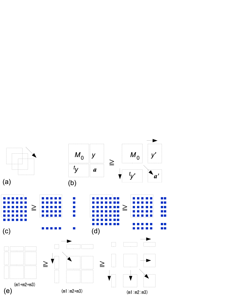
Figure 3: To determine the order of the maximum eigenvalues of the different submatrices (a) a primitive step is to compare submatrices which can be chosen by shifts on the diagonal direction. (b) Another primitive step is to compare submatrices which have the same elements but some of the last block have higher number indices (row and columns). (c) The case with the last one element is shifted. (d) The case with last two elements are shifted. (e) When we compare the submatrices which have many blocks we consider spreading of the largest sub-block such as $m2+m3$, firstly. Then, this submatrix, say (m1;m2+m3), can be connected with another submatrix, say (m1;m2;m3), by considering further spreading of the second largest sub-block such as $m3$.

B.3 Inequalities for the spreading shift

Let us consider the following inequality for the spreading shift depicted in Fig. 3(b)

$$B-B^{\prime} := \left(\begin{array}[]{ccc}M_{0}&y\\ y^{t}&a\\ \end{array}\right)-\left(\begin{array}[]{ccc}M_{0}&y^{\prime}\\ {y^{\prime}}^{t}&a^{\prime}\\ \end{array}\right)\geq 0,$$ (88)

where $M_{0}$, $a$, and $a^{\prime}$ are square matrices. Suppose that the matrices in Eq. (88) are submatrices of $A^{(J)}$ of Eq. (17) and that $J=0$ so that Properties (i) and (ii) are fulfilled. From the decreasing order on the diagonal elements and Property (ii), we can show that the relation of Eq. (88) holds when the final row and column are shifted as in Fig. 3 (c), in which $a$ and $a^{\prime}$ are diagonal elements, and $y$ and $y^{\prime}$ are single column vectors. From the decreasing order on the diagonal and first-off diagonal elements together with Property (ii), we can show that the relation of Eq. (88) holds when the final two rows and two columns are shifted as in Fig. 3(d), (here, $a$ and $a^{\prime}$ are $2\times 2$ matrices). Similarly, we can generate the matrix inequalities in the form of Eq. (88) by using Properties (i) and (ii) for any size of $a$ whenever the diagonal shift ($a\to a^{\prime}$) is in decreasing order.

By further spreading the last lows and columns associated with the position of the square matrix $a$, we can generate inequalities with more separations as in Fig. 3(e). To make three separation $(m1:m2:m3)$, we consider the diagonal shift of the column-length $m2+m3$ square matrix, firstly, and then we spread the last square matrix of the column-length $m3$. We can reach any given separation by repeating these process recursively.

From Properties (i) and (ii), we can see that, for sufficiently larger $n$, the inequalities for the diagonal shift and spreading shift always hold. This is also the case for general $J\neq 0$ since similar properties hold with a bit complicated conditions such as Eq. (62) and Table 1 (See the discussion in Appendix B.1). Hence, the set of submatrices we need to compare the maximum eigenvalues is a finite set of smaller-$n$-index submatrices that could not be connected by the matrix inequalities obtained by these properties. On this basis, the search of the submatrices that have larger maximum eigenvalues can be carried out by a relatively small number of calculation steps. We will present a systematical procedure to identify relevant submatrices in the following.

B.4 Relevant set of submatrices

B.4.1 For $J=0$ and $k=1,2,3,4,5$

Let us suppose that $J=0$. For $k=1,2,3$, the matrix inequalities both in the diagonal shift and the spreading shift of Fig. 3 (a) and (b) hold for any $n\geq 0$. This leads to $\|A_{\{0\}}^{(0)}\|\geq\|A_{\{n\}}^{(0)}\|$ for $k=1$, $\|A_{\{0,1\}}^{(0)}\|\geq\|A_{\{n,n^{\prime}\}}^{(0)}\|$ for $k=2$, and $\|A_{\{0,1,2\}}^{(0)}\|\geq\|A_{\{n,n^{\prime},n^{\prime\prime}\}}^{(0)}\|$ for $k=3$.

For $k=4$, we can show the inequality for the spreading shift $\|A^{(0)}_{\{n,n+1,n+2,n+3\}}\|\geq\|A^{(0)}_{\{n,n+n^{\prime},n+n^{\prime\prime},n+n^{\prime\prime\prime}\}}\|$ by using Property (ii) and the inequalities in the diagonal shift of the $2\times 2$ and $3\times 3$ matrices above. From the row of $l=3$ in Table 1, the inequalities for the diagonal shift is fulfilled whenever $n\geq t_{l}-l=2$. Hence, the only submatrices that could not be connected by the inequalities are $A^{(0)}_{\{0,1,2,3\}}$, $A^{(0)}_{\{1,2,3,4\}}$, and $A^{(0)}_{\{2,3,4,5\}}$. Therefore, the maximum in Eq. (18) is obtained by comparing the first three matrices, i.e. $\max_{n\in\{0,1,2\}}\|A^{(0)}_{\{n,n+1,n+2,n+3\}}\|$.

For $k=5$, we can show the inequality for the spreading shift $\|A^{(0)}_{\{n,n+1,n+2,n+3,n+4\}}\|\geq\|A^{(0)}_{\{n,n+n^{\prime},n+n^{\prime\prime},n+n^{\prime\prime\prime},n+n^{\prime\prime\prime\prime}\}}\|$ by using Property (ii) and the results above except for the case of $n=0$. For $n=0$, we could not have the matrix inequality for $A_{\{0,1,2,3,4\}}^{(0)}$ and $A_{\{0,2,3,4,5\}}^{(0)}$ because the $4\times 4$ matrix inequality could not hold for the first two case of the diagonal shift ($n\geq t_{3}-3=2$). From Property (i) and the results of $k\leq 4$ above, we also have the inequality for the diagonal shift $\|A^{(0)}_{\{n,n+1,n+2,n+3,n+4\}}\|\geq\|A^{(0)}_{\{n+1,n+2,n+3,n+4,n+5\}}\|$ when $n\geq t_{4}-4=5$. In this case, the matrix inequality for the diagonal shift could not hold for the first five $5\times 5$ submatrices $\|A_{\{n,n+1,n+2,n+3,n+4\}}\|$ with ${n\in\{0,1,2,3,4\}}$. Therefore, the optimization can be done by taking the largest one of $\|A_{\{0,2,3,4,5\}}\|$ and $\|A_{\{n,n+1,n+2,n+3,n+4\}}\|$ with ${n\in\{0,1,2,3,4,5\}}$.

B.4.2 For general $J$ and $k$

For temporary simplicity, let us suppose $|J|\leq 4$ [It corresponds to $u^{(J)}=0$ in Eq. (62)]. The set of submatrices which could not be connected by the inequalities for given $k$ can be specified from $t_{k-1},t_{k-2},\cdots,t_{0}$ in Table 1 as follows: First we generate the number of $t_{k-1}-(k-1)+1=t_{k-1}-k+2$ sets of $\vec{n}$ in which the submatrix corresponding to $A_{\vec{n}}$ could not be connected by the inequalities with respect to the diagonal shift:

$$\{0,1,\cdots,k-1\},$$

$$\{1,2,\cdots,k-1,k\},$$

$$\ \ \vdots$$

$$\{t_{k-1}-k,\cdots,t_{k-1}-1\},$$

$$\{t_{k-1}-k+1,\cdots,t_{k-1}\}.$$ (89)

Second, we generate the sets by repeating the diagonal shift of the last $k-1$ elements of each set of Eq. (89) until the last index of $\vec{n}$ fulfills $n_{k}>t_{k-2}$ as

$$\{0,\underbrace{1,\cdots,k-1}_{k-1\ elements}\},\{0,\underbrace{2,3,\cdots,k}_{\to\rm Shifted}\},\{0,\underbrace{3,4,\cdots,k+1}_{\to\rm Shifted}\},\cdots$$

$$\{1,\underbrace{2,\cdots,k-1,k}_{k-1\ \rm elements}\},\{1,\underbrace{3,4,\cdots,k-1,k}_{\to\rm Shifted}\},\{1,\underbrace{4,5,\cdots,k,k+1}_{\to\rm Shifted}\},\cdots$$

$$\vdots$$

$$\{t_{k-1}\!-\!k,\cdots,t_{k-1}\!-\!1\},\{t_{k-1}\!-\!k,t_{k-1}-k+2,\cdots,t_{k-1}\},\cdots$$

$$\{t_{k-1}\!-\!k\!+\!1,\cdots,t_{k-1}\},\{t_{k-1}-\!k\!+\!1,t_{k-1}\!-\!k\!+\!3,\cdots,t_{k\!-\!1}\!+\!1\},\cdots$$

Third and finally, we generate the sets by repeating the diagonal shift of the last $k-2$ elements of each set of Eq. (LABEL:ts) until the last index of $\vec{n}$ fulfills $n_{k}>t_{k-3}$. For example from the elements in the first line of Eq. (LABEL:ts) we have

$$\{0,1,\underbrace{2,\cdots,k-1}_{k-2\ \rm elements}\},\{0,1,\underbrace{3,4,\cdots,k}_{\to\rm Shifted}\},\{0,1,\underbrace{4,5,\cdots,k+1}_{\to\rm Shifted}\},\cdots$$

$$\{0,2,\underbrace{3,4,\cdots,k}_{k-2\ \rm elements}\},\{0,2,\underbrace{4,5,\cdots,k+1}_{\to\rm Shifted}\},\{0,2,\underbrace{5,6,\cdots,k+2}_{\to\rm Shifted}\},\cdots$$

$$\{0,3,\underbrace{4,5,\cdots,k+1}_{k-2\ \rm elements}\},\{0,3,\underbrace{5,6,\cdots,k+2}_{\to\rm Shifted}\},\cdots$$

$$\vdots$$ (91)

In this manner, we can obtain the total number of, at most, $\prod_{l=0}^{k-1}(t_{l}-l-1)$ sets of indices $\vec{n}$.

For the case of $|J|>4$, we modify the generation process by using $u^{(J)}$ of Eq. (62) so that the diagonal shift of the last $l$ elements is repeated until the last index of $\vec{n}$ fulfills $n_{k}>\max\{t_{l-1},u^{(J)}+l-1\}$.

B.5 Outline for numerical calculation

Suppose that $k$, $\kappa$ and $x$ are given. We first search the set of $\{A^{(J)}\}_{J}$ which include $k\times k$ principle submatrices whose trace is grater than the conjectured maximum value $\|A_{\{0,1,2,\cdots,k-1\}}^{(0)}\|$. This process can be executed by only using the diagonal elements of $\{A^{(J)}\}_{J}$.

Next, we determine the relevant submatrices according to the process described in Appendix B.4.2 for relevant $J$.

Lastly, the maximum eigenvalues are directly compared to determine the maximum.

References

- Horodecki et al. (2009) R. Horodecki, P. Horodecki, M. Horodecki, and K. Horodecki, “Quantum entanglement,” Rev. Mod. Phys. 81, 865–942 (2009).
- Pan et al. (2012) J.-W. Pan, Z.-B. Chen, C.-Y. Lu, H. Weinfurter, A. Zeilinger, and M. Żukowski, “Multiphoton entanglement and interferometry,” Rev. Mod. Phys. 84, 777–838 (2012).
- Terhal and Horodecki (2000) B.M. Terhal and P. Horodecki, “Schmidt number for density matrices,” Phys. Rev. A 61, 040301 (2000).
- Huang (2006) S. Huang, “Schmidt number for quantum operations,” Phys. Rev. A 73, 052318 (2006).
- Chruściński and Kossakowski (2006) Dariusz Chruściński and Andrzej Kossakowski, “On partially entanglement breaking channels,” Open Systems & Information Dynamics 13, 17–26 (2006).
- Namiki (2013) R. Namiki, “Composability of partial-entanglement-breaking channels via entanglement-assisted local operations and classical communication,” Phys. Rev. A 88, 064301 (2013).
- Horodecki et al. (2003) M. Horodecki, P. W. Shor, and M. B. Ruskai, “Entanglement Breaking Channels,” Rev. Math. Phys. 15, 629 (2003).
- Holevo (2008) A. S. Holevo, “Entanglement-breaking channels in infinite dimensions,” Probl. Info. Transm. 44, 171–184 (2008).
- Namiki and Tokunaga (2012a) R. Namiki and Y. Tokunaga, “Schmidt-number benchmark for genuine quantum memories and gates,” Phys. Rev. A 85, 010305(R) (2012a).
- Sanpera et al. (2001) A. Sanpera, D. Bruß, and M. Lewenstein, “Schmidt-number witnesses and bound entanglement,” Phys. Rev. A 63, 050301 (2001).
- Tokunaga et al. (2006) Y. Tokunaga, T. Yamamoto, M. Koashi, and N. Imoto, “Fidelity estimation and entanglement verification for experimentally produced four-qubit cluster states,” Phys. Rev. A 74, 020301(R) (2006).
- Tokunaga et al. (2008) Y. Tokunaga, S. Kuwashiro, T. Yamamoto, M. Koashi, and N. Imoto, “Generation of high-fidelity four-photon cluster state and quantum-domain demonstration of one-way quantum computing,” Phys. Rev. Lett. 100, 210501 (2008).
- Inoue et al. (2009) R. Inoue, T. Yonehara, Y. Miyamoto, M. Koashi, and M. Kozuma, “Measuring qutrit-qutrit entanglement of orbital angular momentum states of an atomic ensemble and a photon,” Phys. Rev. Lett. 103, 110503 (2009).
- Li et al. (2010) C.-M. Li, K. Chen, A. Reingruber, Y.-N. Chen, and J.-W. Pan, “Verifying genuine high-order entanglement,” Phys. Rev. Lett. 105, 210504 (2010).
- Sperling and Vogel (2011) J. Sperling and W. Vogel, “Determination of the schmidt number,” Phys. Rev. A 83, 042315 (2011).
- Namiki and Tokunaga (2012b) R. Namiki and Y. Tokunaga, “Discrete fourier-based correlations for entanglement detection,” Phys. Rev. Lett. 108, 230503 (2012b).
- Shahandeh et al. (2013) F. Shahandeh, J. Sperling, and W. Vogel, “Operational Gaussian Schmidt-number witnesses,” Phys. Rev. A 88, 062323 (2013).
- Gutiérrez-Esparza et al. (2014) A. J. Gutiérrez-Esparza, W. M. Pimenta, B. Marques, A. A. Matoso, J. Sperling, W. Vogel, and S. Pádua, “Detection of nonlocal superpositions,” Phys. Rev. A 90, 032328 (2014).
- Braunstein and van Loock (2005) S.L. Braunstein and P. van Loock, “Quantum information with continuous variables,” Rev. Mod. Phys. 77, 513–577 (2005).
- Hammerer et al. (2010) K. Hammerer, A.S. Sørensen, and E.S. Polzik, “Quantum interface between light and atomic ensembles,” Rev. Mod. Phys. 82, 1041–1093 (2010).
- Weedbrook et al. (2012) C. Weedbrook, S. Pirandola, R. García-Patrón, N.J. Cerf, T.C. Ralph, J.H. Shapiro, and S. Lloyd, “Gaussian quantum information,” Rev. Mod. Phys. 84, 621–669 (2012).
- Furusawa et al. (1998) A. Furusawa, J. L. Sørensen, S. L. Braunstein, C. A. Fuchs, H. J. Kimble, and E. S. Polzik, “Unconditional quantum teleportation,” Science 282, 706–710 (1998).
- Julsgaard et al. (2004) Brian Julsgaard, Jacob Sherson, J.~Ignacio Cirac, Jaromir Fiurasek, and Eugene S Polzik, “Experimental demonstration of quantum memory for light,” Nature 432, 482 (2004).
- Lobino et al. (2009) M. Lobino, C. Kupchak, E. Figueroa, and A. I. Lvovsky, “Memory for light as a quantum process,” Phys. Rev. Lett. 102, 203601 (2009).
- Braunstein et al. (2000) S.L. Braunstein, C.A. Fuchs, and H.J. Kimble, “Criteria for continuous-variable quantum teleportation,” J. Mod. Opt. 47, 267 (2000).
- Hammerer et al. (2005) K. Hammerer, M. M. Wolf, E. S. Polzik, and J. I. Cirac, “Quantum benchmark for storage and transmission of coherent states,” Phys. Rev. Lett. 94, 150503 (2005).
- Namiki et al. (2008) R. Namiki, M. Koashi, and N. Imoto, “Fidelity criterion for quantum-domain transmission and storage of coherent states beyond the unit-gain constraint.” Phys. Rev. Lett. 101, 100502 (2008).
- Takano et al. (2008) T. Takano, M. Fuyama, R. Namiki, and Y. Takahashi, “Continuous-variable quantum swapping gate between light and atoms,” Phys. Rev. A 78, 010307(R) (2008).
- Namiki (2011a) R. Namiki, “Fundamental quantum limits on phase-insensitive linear amplification and phase conjugation in a practical framework,” Phys. Rev. A 83, 040302 (2011a).
- Chiribella and Xie (2013) G. Chiribella and J. Xie, “Optimal design and quantum benchmarks for coherent state amplifiers,” Phys. Rev. Lett. 110, 213602 (2013).
- Namiki (2011b) R. Namiki, “Simple proof of the quantum benchmark fidelity for continuous-variable quantum devices,” Phys. Rev. A 83, 042323 (2011b).
- Yang et al. (2014) Y. Yang, G. Chiribella, and G. Adesso, “Certifying quantumness: Benchmarks for the optimal processing of generalized coherent and squeezed states,” Phys. Rev. A 90, 042319 (2014).
- (33) R. Namiki, “Converting separable conditions to entanglement breaking conditions,” arXiv:1503.07109 .
- Fuchs and Sasaki (2003) C. A. Fuchs and M. Sasaki, “Squeezing quantum information through a classical channel: measuring the quantumness of a set of quantum states,” Quantum Inf. Comput. 3, 377 (2003).
- Namiki (2008) R. Namiki, “Verification of the quantum-domain process using two nonorthogonal states,” Phys. Rev. A 78, 032333 (2008).
- Häseler et al. (2008) H. Häseler, T. Moroder, and N. Lütkenhaus, “Testing quantum devices: Practical entanglement verification in bipartite optical systems,” Phys. Rev. A 77, 032303 (2008).
- Häseler and Lütkenhaus (2009) H. Häseler and N. Lütkenhaus, “Probing the quantumness of channels with mixed states,” Phys. Rev. A 80, 042304 (2009).
- Owari et al. (2008) M. Owari, M. B. Plenio, E. S. Polzik, A. Serafini, and M. M. Wolf, “Squeezing the limit: quantum benchmarks for the teleportation and storage of squeezed states,” New J. Phys. 10, 113014 (2008).
- Namiki and Azuma (2015) R. Namiki and K. Azuma, “Quantum benchmark via an uncertainty product of canonical variables,” Phys. Rev. Lett. 114, 140503 (2015).
- Namiki (2015) R. Namiki, “Amplification uncertainty relation for probabilistic amplifiers,” Phys. Rev. A 92, 032326 (2015).
- Killoran and Lütkenhaus (2011) N. Killoran and N. Lütkenhaus, “Strong quantitative benchmarking of quantum optical devices,” Phys. Rev. A 83, 052320 (2011).
- Killoran et al. (2012) N. Killoran, M. Hosseini, B. C. Buchler, P. K. Lam, and N. Lütkenhaus, “Quantum benchmarking with realistic states of light,” Phys. Rev. A 86, 022331 (2012).
- Khan et al. (2013) I. Khan, C. Wittmann, N. Jain, N. Killoran, N. Lütkenhaus, C. Marquardt, and G. Leuchs, “Optimal working points for continuous-variable quantum channels,” Phys. Rev. A 88, 010302 (2013).
- Shirokov (2013) M.E. Shirokov, “Schmidt number and partially entanglement-breaking channels in infinite-dimensional quantum systems,” Mathematical Notes 93, 766–779 (2013).
- Yukawa et al. (2008) M. Yukawa, H. Benichi, and A. Furusawa, “High-fidelity continuous-variable quantum teleportation toward multistep quantum operations,” Phys. Rev. A 77, 022314 (2008).
- Pirandola et al. (2015) S. Pirandola, J. Eisert, C. Weedbrook, A. Furusawa, and S. L. Braunstein, “Advances in quantum teleportation,” Nature Photonics 9, 641–652 (2015).
- (47) T.C. Ralph and A.P. Lund, “Nondeterministic noiseless linear amplification of quantum systems,” Quantum Communication Measurement and Computing Proceedings of 9th International Conference, Ed. A. Lvovsky, 155 (AIP, New York 2009), arXiv:0809.0326v1 .
- Chrzanowski et al. (2014) H.M. Chrzanowski, N. Walk, S.M. Assad, J. Janousek, S. Hosseini, T.C. Ralph, T. Symul, and P.K. Lam, “Measurement-based noiseless linear amplification for quantum communication,” Nature Photonics 8, 333–338 (2014).
- Xiang et al. (2010) G. Y. Xiang, T. C. Ralph, A. P. Lund, N. Walk, and G. J. Pryde, “Heralded noiseless linear amplification and distillation of entanglement,” Nature Photonics 4, 316–319 (2010).
- Neergaard-Nielsen et al. (2013) J.S. Neergaard-Nielsen, Y. Eto, C.W. Lee, H. Jeong, and M. Sasaki, “Quantum tele-amplification with a continuous-variable superposition state,” Nature Photonics 7, 439–443 (2013).
- Horn and Johnson (2007) R.A. Horn and C.R. Johnson, Matrix Analysis (Cambridge, NewYork, 2007).