Flows in Flatland: A Romance of Few Dimensions

Abstract.

In this paper, we present our general results about traversing flows on manifolds with boundary in the context of the flows on surfaces with boundary. We take advantage of the relative simplicity of $2D$-worlds to explain and popularize our approach to the Morse theory on smooth manifolds with boundary, in which the boundary effects take the central stage.

1. Introduction

This paper is about the gradient flows on compact surfaces, thus the reference to Abbott’s Flatland [Ab] in the title. The paper is an informal introduction into the philosophy and some key results from [K] -[K6], as they manifest themselves in $2D$.

The remarkable convergence of topological, geometrical, and analytical approaches to the study of closed surfaces is widely recognized by the practitioners for more than a century. We will exhibit a similar convergence of different investigative approaches to vector flows on surfaces with boundary.

We will take advantage of the relative simplicity of $2D$ flows to illustrate and popularize the main ideas of our recent research of traversally generic flows on manifolds with boundary. When the results are specific to the dimension two, their validation will be presented in detail. The multidimensional arguments that resist significant simplifications in $2D$ will be described and explained in general terms.

Throughout the investigation, we focus on the interactions of gradient flows with the boundary, rather than on the critical points of Morse functions. So, in our approach to the Morse Theory, the boundary effects rule.

2. On Morse Theory on surfaces with boundary and beyond

Morse Theory, the classical book of John W. Milnor [Mi], starts with the canonical picture of a Morse function $f:T^{2}\to\mathbb{R}$ on a 2-dimensional torus $T^{2}$ (see Fig. 1). It is portrayed as the height function $f$ on the torus $T^{2}$ residing in the space $\mathbb{R}^{3}$. The height $f$ has four critical points: $a,b,c$, and $d$ so that

$$f(a)>f(b)>f(c)>f(d).$$

A point $z$ is called critical if the differential $df$ of $f$ vanishes at $z$. In the vicinity of each critical point $z$, $T^{2}$ admits a pair of local coordinate functions, say $x$ and $y$, so that locally the function $f$ acquires the form

$$f(x,y)=f(0,0)\pm x^{2}\pm y^{2},$$

where the signs may form four possible combinations.

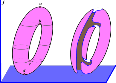
Figure 1. A Morse function $f$ on a 2-dimensional torus $T^{2}$ and its non-singular restriction to the complement $X$ of a disk $D^{2}\subset T^{2}$. Note the curved geometry of the boundary loop $\partial X$ which “remembers” the nature of $f$-critical points $a,b,c,d$.

We call a vector field $v$, tangent to $T^{2}$, gradient-like if $df(v)>0$ everywhere outside of the set $Cr(f)$ of critical points.

If the torus is “slightly slanted” with respect to the vertical coordinate $f$ in $\mathbb{R}^{3}$, then the following picture emerges. The majority of downward trajectories of the $f$-gradient flow $\{\Phi_{t}\}_{t\in\mathbb{R}}$ that emanate from $a$, asymptotically reach $d$. There are two trajectories that asymptotically link $a$ with $b$, and two trajectories that link $a$ with $c$. No (unbroken) trajectory asymptotically connects $b$ to $c$.

Perhaps, a more transparent depiction of the gradient flow $\{\Phi_{t}\}_{t\in\mathbb{R}}$ is given in Fig. 2, where the torus is shown in terms of its fundamental domain, the square. To form $T^{2}$, the opposite sides of the square are identified in pairs.

The Morse Theory is concerned with the sets of constant level $\{f^{-1}(\alpha)\}_{\alpha\in\mathbb{R}}$ and the below constant level sets $\{f^{-1}((-\infty,\alpha))\}_{\alpha\in\mathbb{R}}$. The main observation is that the topology of these sets is changing in an essential way only when the rising $\alpha$ crosses the critical values

$$Cr(f)=\{f(a),f(b),f(c),f(d)\}.$$

Each such “critical crossing” results in an elementary surgery on the set $\{f^{-1}((-\infty,\alpha))\}_{\alpha\in\mathbb{R}}$, where $\alpha$ is just below a critical value $\alpha_{\star}\in Cr(f)$. For a small $\epsilon>0$, an elementary surgery

$$f^{-1}((-\infty,\alpha_{\star}-\epsilon))\Rightarrow f^{-1}((-\infty,\alpha_{\star}+\epsilon))$$

attaches the handle $f^{-1}((\alpha_{\star}-\epsilon,\alpha_{\star}+\epsilon))$ to the set $f^{-1}((-\infty,\alpha-\epsilon))$. Eventually, when $\alpha$ rises above $f(a)$, the entire topology of torus $T^{2}$ is captured by a sequence of these elementary surgeries.

From a different angle, the knowledge of how the critical points $a,b,c,d$ interact via the trajectories of the $\Phi_{t}$-flow is also sufficient for reconstructing the surface $T^{2}$ as Fig. 2 suggests (see [C]).

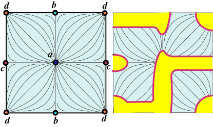
Figure 2. The gradient flow of the Morse function $f:T^{2}\to\mathbb{R}$ from Fig. 1 and its restriction to the complement of a disk in the torus.

Note that, in the vicinity of each critical point, the gradient flow exhibits discontinuity: small changes in the initial position of a point $z$, residing in the vicinity of a critical point, result in significant differences in the position of $\Phi_{t}(z)$ for big positive/small negative values of $t$ (see Fig. 3). In fact, this discontinuity of the gradient flow, expressed in terms of the stable and unstable manifolds of critical points (see [Mi]), captures the topology of the surface (as the left diagram in Fig. 2 suggests)!

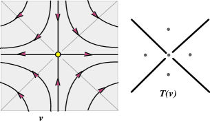
Figure 3. A gradient flow $v$ in the vicinity of a singular point and a very schematic picture of its (nonseparable) trajectory space $\mathcal{T}(v)$.

As a result of gradient flow discontinuity, the space of trajectories $\mathcal{T}(v)$ is pathological (non-separable). The space $\mathcal{T}(v)$ is constructed by declaring equivalent any two points that reside on the same trajectory.

When a compact connected surface $X$ has a nonempty boundary $\partial X$, traditionally, the Morse function $f:X\to\mathbb{R}$ is assumed to be constant on $\partial X$ and its gradient flow interacts with the boundary in constrained way. Then the relative topology of the pair $(X,\partial X)$ can be captured in the ways analogous to the previous description of the Morse Theory on torus. In fact, the Morse Theory on manifolds with boundary can be viewed as a very special instance of the Morse Theory on stratified spaces (the two strata $\partial X$ and $X$ form the stratification). The latter was developed by Goresky and MacPherson in [GM] -[GM2].

In this paper, we propose a different philosophy for the Morse Theory on compact surfaces/manifolds $X$ with boundary. To formulate it, let us revisit our favorite closed surface, the torus. By deleting from $T^{2}$ small disks, centered on the points of the critical set $Cr(f)$, we manufacture a surface $X$ whose boundary is a disjoint union of four circles. Evidently, $f:X\to\mathbb{R}$ has no critical points at all. Still it has a nontrivial topology! Can this topology be reconstructed from some data, provided by the critical point-free $f$ and its gradient-like field $v\neq 0$? An experienced reader would notice that the restriction $f|:\partial X\to\mathbb{R}$ has critical points (maxima and minima), some of which interact along the boundary (with the help of a gradient-like field $v^{\partial}$, tangent to $\partial X$). However, it is quite clear that these interactions are not sufficient for a reconstruction of the topology of $X$! In fact, a reconstruction of the surface $X$ becomes possible if one introduces additional interactions between the points of $Cr(f|_{\partial X})$ that occur “through the bulk $X$” and are defined with the help of both vector fields $v$ and $v^{\partial}$. This observation has been explored by a number of authors, but it is not the world view that we are promoting here…

To dramatize further the situation we are facing, let us place four small disks, centered on the critical points of $f:T^{2}\to\mathbb{R}$, into a single open disk $D^{2}$ and form $X=T^{2}\setminus D^{2}$ (see Fig 2, the right diagram). Again, $f|:X\to\mathbb{R}$ has no critical points, the gradient field $v|_{X}\neq 0$, but its topology of $X$ is nontrivial. This time, the boundary $\partial X$ of the punctured torus $X$ is just a single circle! Let us keep this challenge in mind.

Can one propose a “Morse Theory” that is not centered on critical points? The answer is affirmative. It relies on the following observation. Typically, in the vicinity of $\partial X$, the $v$-trajectories are interacting with the boundary in a number of very particular and stable ways: they are either transversal to $\partial X$, or are tangent to it in a concave or convex fashion (see Fig. 5). So the boundary $X$ may be “wiggly” with respect to the flow. We claim that this geometry of the $v$-flow in connection to the boundary $\partial X$ is the crucial ingredient for reconstructions of $X$ in terms of the flow (see Section 8, especially Theorem 8.1).

In the vicinity of a concave tangency point, the $v$-flow is discontinuous in the same sense as the gradient flow is discontinuous in the vicinity of its critical point: in time, close initial points become distant. In this context, the divergence of initially close points occurs due to very different travel times available to them; unlike the infinite travel time for the gradient flows of the Morse theory on closed surfaces, in the case of the non-singular gradient flows on surfaces with boundary, every point exits the surface in finite time. In particular, the surface is not flow-invariant. And again, these discontinuities of the flow reflect the topology of the surface. Let us clarify this point.

Fig. 4 shows a gradient flow $v$ on a surface $X\subset\mathbb{R}^{2}$, the disk with $4$ holes. The nonsingular function $f:X\to\mathbb{R}$ is the vertical coordinate in $\mathbb{R}^{2}$. Each $v$-trajectory is either a closed segment, or a singleton. By collapsing each trajectory to a point, we create a quotient space $\mathcal{T}(v)$ of trajectories. Since the flow trajectories are closed segments or singletons, this time, the trajectory space $\mathcal{T}(v)$ is “decent”, a finite graph with verticies of valency $1$ or $3$ only. The verticies of valency $3$ correspond to the points on $\partial X$ where the boundary is concave with respect to the flow, and the univalent verticies to the points on $\partial X$ where the flow is convex.

The obvious map $\Gamma:X\to\mathcal{T}(v)$ cellular. Moreover, because the fibers of $\Gamma$ are contractable, $\Gamma$ is a homotopy equivalence. In particular, the fundamental groups $\pi_{1}(X)$ and $\pi_{1}(\mathcal{T}(v))$ are isomorphic with the help of $\Gamma$. So the trajectory spaces of generic non-vanishing vector fields $v$ of the gradient type on connected surfaces $X$ with boundary deliver $1$-dimensional homotopy theoretical models of $X$.

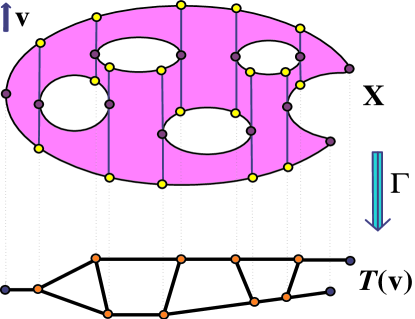
Figure 4. The map $\Gamma:X\to\mathcal{T}(v)$ for a traversally generic (vertical) field $v$ on a disk with $4$ holes. The trajectory space $\mathcal{T}(v)$ is a graph whose verticies are of valecies $1$ and $3$.

3. Vector felds and Morse stratifications on surfaces

Following [Mo], for any vector field $v$ on a compact surface $X$ with boundary such that $v|_{\partial X}\neq 0$, we consider the closed locus $\partial_{1}^{+}X(v)$, where the field is pointing inside $X$ and the closed locus $\partial_{1}^{-}X(v)$, where it points outside. The intersection

$$\partial_{2}X(v)=_{\mathsf{def}}\partial_{1}^{+}X(v)\cap\partial_{1}^{+}X(v)$$

is the locus where $v$ is tangent to the boundary $\partial X$. Points $z\in\partial_{2}X(v)$ come in two flavors: by definition, $z\in\partial^{+}_{2}X(v)$ when $v(z)$ points inside of the locus $\partial_{1}^{+}X(v)$; otherwise $z\in\partial^{-}_{2}X(v)$. To achieve some uniformity of notations, put $\partial_{0}^{+}X=_{\mathsf{def}}X$ and $\partial_{1}X=_{\mathsf{def}}\partial X$.

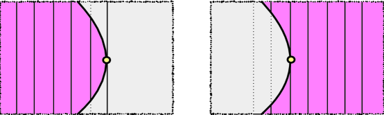
Figure 5. A boundary generic field $v$ in the vicinity of a point from $\partial_{2}^{-}X(v)$ (on the left) and in the vicinity of a point from $\partial_{2}^{+}X(v)$ (on the right).

Definition 3.1.

We say that a vector field $v$ on a compact surface $X$ is boundary generic if:

• $v|_{\partial X}$, viewed as a section of the normal $1$-dimensional (quotient) bundle

  $$n_{1}=_{\mathsf{def}}T(X)|_{\partial X}\big{/}T(\partial X),$$

  is transversal to its zero section,

• $v|_{\partial_{2}X(v)}$, viewed as a section of the normal $1$-dimensional bundle $n_{2}=_{\mathsf{def}}T(\partial X)|_{\partial X}$, is transversal to its zero section. $\diamondsuit$

In particular, for a boundary generic $v$, the loci $\partial_{1}^{\pm}X(v)$ are finite unions of closed intervals and circles, residing in $\partial X$; and the loci $\partial_{2}^{\pm}X(v)$ are finite unions of points, residing in $\partial X$ (see Fig. 4).

We denote by $\mathcal{V}^{\dagger}(X)$ the space (in the $C^{\infty}$-topology) of all boundary generic fields on a compact surface $X$.

Let $\chi(Z)$ denote the Euler number of a space $Z$. Recall that $\chi(Z)$ is the alternating sum of dimensions of the homology spaces $\{H_{i}(Z;\mathbb{R})\}_{i}$.

Since for a connected surface $X$ with boundary $H_{2}(X;\mathbb{R})=0$, we get

$$\chi(X)=1-\dim_{\mathbb{R}}(H_{1}(X;\mathbb{R})).$$

For a closed connected surface,

$$\chi(X)=2-\dim_{\mathbb{R}}(H_{1}(X;\mathbb{R})).$$

Given a vector field $v$ with isolated zeros, we can associate an integer $\mathsf{ind}_{x}(v)$ with each zero $x$ of $v$. This integer is the degree of the map which, crudely speaking, takes each point $z$ on a small circle $C_{x}$ with its center at $x$ to the unit vector $v(z)/\|v(z)\|$. Then we define $\mathsf{Ind}(v)$, the (global) index of $v$, as the sum $\sum_{\{x\in\text{ zeros of }v\}}\mathsf{ind}_{x}(v)$.

The Morse formula [Mo], in the center of our investigation, computes the index $\mathsf{Ind}(v)$ of a given boundary generic vector field $v$ on a surface $X$ as the alternating sum of the Euler numbers of the Morse strata $\{\partial_{j}^{+}X(v)\}_{0\leq j\leq 2}$:

(3.1) $$\mathsf{Ind}(v)=\chi(X)-\chi(\partial_{1}^{+}X(v))+\chi(\partial_{2}^{+}X(v)).$$

In the case of a connected surface $X$ with boundary, $\chi(X)=1-\dim_{\mathbb{R}}(H_{1}(X;\mathbb{R}))$, and this formula reduces to

$$\mathsf{Ind}(v)=1-\dim_{\mathbb{R}}(H_{1}(X;\mathbb{R}))-\#\{\mathsf{arcs}\;in\;\partial_{1}^{+}X(v)\}+\#\{\partial_{2}^{+}X(v)\}$$

$$=1-\dim_{\mathbb{R}}(H_{1}(X;\mathbb{R}))+\frac{1}{2}\big{(}\#\{\partial_{2}^{+}X(v)\}-\#\{\partial_{2}^{-}X(v)\}\big{)}.$$

In particular, if $v\neq 0$, then $\mathsf{Ind}(v)=0$, and we get

(3.2) $$\frac{1}{2}\big{(}\#\{\partial_{2}^{+}X(v)\}-\#\{\partial_{2}^{-}X(v)\}\big{)}=\dim_{\mathbb{R}}(H_{1}(X;\mathbb{R}))-1,$$

where the RHS of the equation is the topological invariant $|\chi(X)|=-\chi(X)$ of $X$. In contrast, the cardinality $\#\{\partial_{2}^{+}X(v)\}$ depends on $v$.

Lemma 3.1.

Let a surface $X$ be formed by removing $k$ open disks from a closed surface $Y$, the sphere with $g$ handles. Then, for any boundary generic field $v\neq 0$ on $X$,

$$\#\{\partial_{2}^{+}X(v)\}\,\geq\,4g-4+2k.$$

Moreover, $\#\{\partial_{2}^{+}X(v)\}=4g-4+2k$ only when $\#\{\partial_{2}^{-}X(v)\}=0$.

Proof.

The Euler number is additive under gluing surfaces along their boundary components. Therefore, if $k$ disks are removed from $Y$, the sphere with $g$ handles, then $\chi(X)=2-2g-k$. Thus the Morse formulas (3.1) and (3.2) imply

$$\#\{\partial_{2}^{+}X(v)\}\geq 4g-4+2k$$

for any $v\neq 0$. Moreover, $\#\{\partial_{2}^{+}X(v)\}=4g-4+2k$ if and only if $\#\{\partial_{2}^{-}X(v)\}=0$, the main feature of the boundary concave fields (see Definition 4.1). ∎

In particular, for any non-vanishing boundary generic field $v$ on a torus with a single hole, $\#\{\partial_{2}^{+}X(v)\}\geq 2$ (cf. Fig. 2).

Recall that an immersion is a smooth map of manifolds, whose differential has the trivial kernel.

Consider a smooth map $\alpha:X\to\mathbb{R}^{2}$, which is an immersion in the vicinity of $\partial X$. Any such $\alpha$ gives rise to the Gauss map $G:\partial X\to S^{1}$, defined by the formula $G(x)=\alpha_{\ast}(\tau_{x})/\|\alpha_{\ast}(\tau_{x})\|$, where $\tau_{x}$ is the tangent vector to $\partial X$ at $x$. The direction of $\tau_{x}$ is consistent with the preferred orientation of $\partial X$, induced by the preferred orientation of $X$ .

Let $\hat{v}\neq 0$ be a constant field on $\mathbb{R}^{2}$. Since the kernel of the differential of $D\alpha:TX\to T\mathbb{R}^{2}$ is trivial along $\partial X$, the field $\hat{v}$ defines a vector field $\tilde{v}=\alpha^{\ast}(\hat{v})$ on $X$ in the vicinity of $\partial X$. The pull-back field $\tilde{v}$ extends to a vector field $v$ on $X$, possibly with zeros (see [G] for engaging discussions of vector field transfers and the Gauss-Bonnet Theorem).

Then the degree of the Gauss map is given by a classical Hopf formula ([H])

$$\deg(G)=\chi(X)-\mathsf{Ind}(v).$$

When $\alpha:X\to\mathbb{R}^{2}$ is an immersion everywhere, the pull-back field $v=\alpha^{\ast}(\hat{v})\neq 0$ everywhere. Thus $\mathsf{Ind}(v)=0$, and, for a connected $X$ with $\partial X\neq\emptyset$, we get

$$\deg(G)=\chi(X)=_{\mathsf{def}}1-\dim(H_{1}(X;\mathbb{R})).$$

So, for an immersions $\alpha$, we get a new interpretation of formula (3.2):

(3.3) $$\deg(G)=\chi(X)=\frac{1}{2}\Big{(}\#\{\partial_{2}^{-}X(v)\}-\#\{\partial_{2}^{+}X(v)\}\Big{)}.$$

This global-to-local formula has another classical geometrical interpretation. Let $\mathsf{g}=\alpha^{\ast}(\mathsf{g}_{E})$ be the Riemannian metric on $X$, the pull-back of the Euclidean metric on $\mathbb{R}^{2}$. Let $K_{\nu}$ denote the normal curvature of $\partial X$ with respect to $\mathsf{g}$. Then

$$\deg(G)=\frac{1}{2\pi}\int_{\partial X}K_{\nu}\,d\mathsf{g},$$

which leads to another pleasing global-to-local connection:

$$\frac{1}{\pi}\int_{\partial X}K_{\nu}\,d\mathsf{g}=\#\{\partial_{2}^{-}X(v)\}-\#\{\partial_{2}^{+}X(v)\}.$$

In particular, for a connected orientable surface $X$ of genus $g$ with a single boundary component,

(3.4) $$\chi(X)=1-2g=\frac{1}{2}\big{(}\#\{\partial_{2}^{-}X(v)\}-\#\{\partial_{2}^{+}X(v)\}\big{)}.$$

So the number of $v$-trajectories $\gamma$ in $X$ that are tangent to $\partial X$, but are not singletons (they correspond to points of $\partial_{2}^{+}X(v)$), as a function of genus $g$, grows at least as fast as $4g-2$!

On the other hand, when $\partial X$ is connected, by the Whitney index formula [W], the degree of the Gauss map $G:\partial X\to S^{1}$ can be also calculated as $\mu+N^{+}-N^{-}$, where $N^{\pm}$ denotes the number of positive/negative self-intersections of the curve $\alpha(\partial X)\subset\mathbb{R}^{2}$, and $\mu=\pm 1$. Here is a brief description of the rule by which the self-intersections acquire polarities. Let $p\in\alpha(\partial X)$ be a point where the coordinate function $y:\mathbb{R}^{2}\to\mathbb{R}$ attends its minimum on the curve $\alpha(\partial X)$. If the tangent vector $\tau_{p}$ at $p$, which defines the orientation of $\alpha(\partial X)$, is $\partial_{x}$, then we put $\mu=+1$; if $\tau_{p}=-\partial_{x}$, then $\mu=-1$. Starting at $p$ and moving in the direction of $\tau_{p}$, we visit each self-intersection $a$ twice and in a particular order. The first visitation defines a tangent vector $\tau_{1}(a)$, the second visitation defines a tangent vector $\tau_{2}(a)$. When the ordered pair $(\tau_{1}(a),\tau_{2}(a))$ defines the clockwise orientation of the $xy$-plane, then we attach “$-$” to $a$. Otherwise, the polarity of $a$ is “$+$”.

Therefore we get a somewhat mysterious connection between the self-intersections of $\partial X$ under immersions $\alpha:X\to\mathbb{R}^{2}$ and the tangency patterns of the flows in $X$ that are the $\alpha$-pull-backs of non-vanishing flows in the plane.

Theorem 3.1.

Let $\hat{v}\neq 0$ be a vector field in the plane $\mathbb{R}^{2}$. Let $X$ be a connected orientable surface with a connected boundary. Consider an immersion $\alpha:X\to\mathbb{R}^{2}$ such that the loop $\alpha(\partial X)$ has transversal self-intersections only. Assume that the pull-back $v=\alpha^{\ast}(\hat{v})$ is a boundary generic field on $X$. Then

$$\frac{1}{2}\Big{(}\#\{\partial_{2}^{+}X(v)\}-\#\{\partial_{2}^{-}X(v)\}\Big{)}=N^{+}-N^{-}\pm 1=2g-1,$$

$$\frac{1}{2}\Big{(}\#\{\partial_{2}^{+}X(v)\}-\#\{\partial_{2}^{-}X(v)\}\Big{)}+2\,\leq N^{+}+N^{-},$$

the latter inequality being sharp by an appropriate choice of $\alpha$.

Proof.

The first formula is the result of combining the Whitney formula for $\deg(G)$ with formulas (3.3), (3.4).

By a theorem of Guth [Gu], for any immersion $\alpha:X\to\mathbb{R}^{2}$, the total number of self-intersections of the loop $\alpha(\partial X)$ admits an estimate

$$N^{+}+N^{-}\geq\,2g+2.$$

Moreover, this lower bound is realized by an immersion $\alpha:X\to\mathbb{R}^{2}$! Therefore, by formula (3.4), the Guth inequality is transformed into

$$N^{+}+N^{-}\geq 2+\frac{1}{2}\big{(}\#\{\partial_{2}^{+}X(v)\}-\#\{\partial_{2}^{-}X(v)\}\big{)}.$$

Moreover, for some optimal immersion $\alpha$,

$$N^{+}+N^{-}=2+\frac{1}{2}\big{(}\#\{\partial_{2}^{+}X(v)\}-\#\{\partial_{2}^{-}X(v)\}\big{)}=2-\frac{1}{2\pi}\int_{\partial X}K_{\nu}\,d\mathsf{g}.$$

∎

When a surface $X$ is oriented and a field $v$ is boundary generic, then the points from $\partial_{2}^{+}X(v)$ come in two new flavors: “$\oplus,\ominus$”. By definition, a point $a\in\partial_{2}^{+}X(v)$ has the polarity “$\oplus$” if the orientation of $T_{a}X$ determined by the pair $(\nu_{a},v(a))$, where $\nu_{a}$ is the inner normal to $\partial X$, agrees with the preferred orientation of $X$. Otherwise, the polarity of $a$ is defined to be “$\ominus$”.

Thus, for each choice of orientation of $X$ (and hence of $\partial X$) we get a partition

$$\partial_{2}^{+}X(v)=\partial_{2}^{+,\oplus}X(v)\coprod\partial_{2}^{+,\ominus}X(v).$$

Switching the orientation of $X$ switches the second polarities in the partition.

4. Convexity, concavity, and complexity of flows in 2D

Definition 4.1.

We say that a boundary generic vector field $v$ is boundary convex if $\partial_{2}^{+}X(v)=\emptyset$. We say that a boundary generic $v$ is boundary concave if $\partial_{2}^{-}X(v)=\emptyset$ (see Fig 5). $\diamondsuit$

The existence of a boundary convex field puts severe restrictions on the topology of the surface.

Lemma 4.1.

If a compact connected surface $X$ with boundary $\partial X\neq\emptyset$ admits a boundary convex gradient-like vector field $v\neq 0$, then $X$ is either a disk $D^{2}$, or an annulus $A^{2}$.

Proof.

The convexity of the field $v$ implies that $X$ admits a $(-v)$-directed continuous retraction on the locus $\partial_{1}^{+}X(v)$. Since $X$ is connected, it follows that $\partial_{1}^{+}X(v)$ is connected as well. Thus, $\partial_{1}^{+}X(v)$ is either a circle, or a segment. In the first case, $X$ is diffeomorphic to an annulus $S^{1}\times[0,1]$; in the second case, $X$ is diffeomorphic to a disk $D^{2}$. ∎

The same phenomenon occurs in any dimension: if a compact connected smooth $(n+1)$-manifold $X$ with a connected boundary admits a boundary convex gradient-like vector field $v\neq 0$, then $H_{n}(X;\mathbb{Z})=0$ ([K1]). In other words, $H_{n}(X;\mathbb{Z})\neq 0$ is a topological obstruction to the existence of a boundary convex non-vanishing gradient field on $X$.

In contrast, the boundary concave non-vanishing gradient fields are plentiful. For example, consider a radial vector field $v$ on an annulus $A^{2}$. Delete from $A^{2}$ any number of convex disks and restrict $v$ to the resulting $2$-disk with holes. The convexity of the disks that we have removed implies that any disk with holes admits a boundary concave gradient-like vector $v\neq 0$.

Many other surfaces admit such concave fields as well. For example, consider a Morse function $f:Y\to\mathbb{R}$ on a closed surface $Y$ and its gradient field $v$. Then removing small convex (in the local Morse coordinates) balls, centered on the critical points, from $Y$, produces a boundary concave non-vanishing gradient field on $X$. In particular if $Y$ is a sphere with $g$ handles, then one can find a Morse function with $2g+2$ critical points (see Fig. 1). So the surface $X$, obtained from $Y$ by removing $2g+2$ balls, admits a concave gradient-like field $v\neq 0$.

In fact, by Theorem 6.2, any connected orientable surface with boundary, but the disk, admits a boundary concave non-vanishing gradient field!

We view the integer $c^{+}(v)=_{\mathsf{def}}\#(\partial_{2}^{+}X(v))$ as a measure of complexity of the $v$-flow, subject to the condition $\mathsf{Ind}(v)=0$ or, alternatively, subject to the condition $v\neq 0$ .

We define the complexity of a compact connected surface $X$ with boundary as the minimum

$$c^{+}(X)=\min_{v\neq 0}\{c^{+}_{2}(v)\},$$

where $v$ runs over all non-vanishing boundary generic fields on $X$.

By varying $v$ within different spaces of fields, one may consider a variety of such minima; non-vanishing fields and non-vanishing gradient-like fields are the two most important cases. So we introduce the gradient complexity

$$gc^{+}(X)=_{\mathsf{def}}\min_{v\neq 0\;\text{of the gradient type}}\{c^{+}_{2}(v)\},$$

where $v$ runs over all non-vanishing gradient-like fields on $X$.

Evidently $gc^{+}(X)\geq c^{+}(X)$. Let $M^{\circ}$ denote the Möbius band. In Section 6, we will show that $gc^{+}(M^{\circ})=1$, while $c^{+}(M^{\circ})=0$, so the two notions of complexity are different.

In terms of this complexity, we can restate the Lemma 3.1 as follows.

Corollary 4.1.

Let $X$ be a connected compact surface with boundary. Let $v$ be a boundary generic vector field on $X$, subject to the condition $\mathsf{Ind}(v)=0$.

Then the complexity of $v$ satisfies the inequality

$$c^{+}(v)\geq 2\cdot\dim_{\mathbb{R}}H_{1}(X;\mathbb{R})-2=-2\cdot\chi(X).$$

When $\chi(X)\leq 0$, this inequality turns into the equality $c^{+}(v)=-2\cdot\chi(X)$ if and only if $v$ is boundary concave.

As a result, for any natural $N$, there are finitely many connected compact surfaces of bounded complexity $c^{+}(X)\leq N$. In fact, the number of such surfaces (counted up to a homeomorphism) grows as a quadratic function in $N$. $\diamondsuit$

Example 4.1. For any non-vanishing boundary concave field $v$ on the torus with a single hole, $\#\{\partial_{2}^{+}X(v)\}=2$. In fact, the constant field $v$, being restricted to the complement to a convex disk in $T^{2}$, is boundary concave and has the property $\#\{\partial_{2}^{+}X(v)\}=2$. Thus, by Corollary 4.1, $c^{+}(X)=2$. $\diamondsuit$

Lemma 3.1 leads immediately to

Corollary 4.2.

Let $X$ be a sphere with $g$ handles and $k$ holes, where $g,k\geq 1$. If $X$ admits a non-vanishing boundary concave field $v$, then $\#\{\partial_{2}^{+}X(v)\}=4g-4+2k$. $\diamondsuit$

Given a compact surface $X$ with boundary, we form its double $DX=_{\mathsf{def}}X\cup_{\partial X}X$ by attaching two copies of $X$ along their boundaries. Note that $\chi(DX)=2\cdot\chi(X)$. Therefore, $\chi(X)<0$ if and only if $\chi(DX)<0$.

Recall that any closed orientable surface with a negative Euler number admits a metric of constant negative curvature $-1$. So if $\chi(X)<0$, then $DX$ admits such hyperbolic metric.

Let $vol(DX)$ denote the hyperbolic volume of $DX$, and let $vol(\Delta^{2})$ denote the volume of an ideal hyperbolic triangle $\Delta^{2}$ in the hyperbolic plane $\mathbf{H}^{2}$.

In $2D$, a remarkable convergence of topology and geometry takes place. In the spirit of this convergence, since $\chi(DX)=-vol(DX)/vol(\Delta^{2})$, Corollary 4.1 admits a more geometric reformulation:

Theorem 4.1.

Let $v\neq 0$ be a boundary generic vector field on a compact connected and orientable surface $X$ with boundary. Assume that $\chi(X)<0$. Then the complexity of the $v$-flow satisfies the inequality:

$$c^{+}(v)\;\geq\;vol(DX)/vol(\Delta^{2}).$$

Moreover, $c^{+}(v)=vol(DX)/vol(\Delta^{2})$ if and only if $v$ is boundary concave. $\diamondsuit$

Theorem 4.1 admits far reaching multidimensional generalizations (see [AK], [K5]). They are valid for so called traversally generic vector fields (see Definitions 5.1 and 5.2 and [K2]) on arbitrary smooth compact $(n+1)$-dimensional manifolds $X$ with boundary. Such fields $v$ naturally generate stratifications of trajectory spaces $\mathcal{T}(v)$, whose strata are labeled by the combinatorial patterns of tangency from the universal partially ordered set $\Omega^{\bullet}_{{}^{\prime}\langle n]}$ (see the end of Section 6 and [K3]). In high dimensions, we use the simplicial semi-norms $\|\sim\|_{\Delta}$ of Gromov [Gr] on the homology $H_{\ast}(X;\mathbb{R})$ and $H_{\ast}(DX;\mathbb{R})$ (as a substitute of the hyperbolic volume) to provide lower bounds on the number of connected components of the $\Omega^{\bullet}_{{}^{\prime}\langle n]}$-strata of any given dimension.

5. On spaces of vector fields

Definition 5.1.

We say that a vector field $v\neq 0$ on a compact surface $X$ is traversing if all its trajectories are closed segments or singletons. $\diamondsuit$

Each trajectory $\gamma$ of a traversing field $v$ must reach the boundary both in positive and negative times: otherwise $\gamma$ is not homeomorphic to a closed interval.

We denote by $\mathcal{V}_{\mathsf{trav}}(X)$ the space (in the $C^{\infty}$-topology) of all traversing fields on $X$.

We denote by $\mathcal{V}_{\mathsf{grad}}(X)$ the space (in the $C^{\infty}$-topology) of all gradient-like fields on a given compact surface $X$ and by $\mathcal{V}_{\neq 0}(X)$ the space of all non-vanishing fields on $X$.

The next lemma says that $v$ is traversal if and only if it is non-vanishing and of a gradient type (see [K1] for the proof).

Lemma 5.1.

For any compact connected surface $X$ with boundary,

$$\mathcal{V}_{\mathsf{trav}}(X)=\mathcal{V}_{\mathsf{grad}}(X)\cap\mathcal{V}_{\neq 0}(X).$$

$\diamondsuit$

The surfaces $X$ and vector fields $v$ we consider are all smooth. We can add an external collar to $X$ to form a diffeomorphic surface $\hat{X}\supset X$ and to extend $v$ to a smooth field $\hat{v}$ on $\hat{X}$. Let $\hat{\gamma}$ be a $\hat{v}$-trajectory (or rather its germ) through a point $x$ of $\partial X$. We can talk about order of tangency of two smooth curves, $\hat{\gamma}$ and $\partial X$, at $x\in\hat{\gamma}\cap\partial X$ in $\hat{X}$ (see Definition 7.1). We say that the tangency of $\hat{\gamma}$ to $\partial X$ is simple if its degree is 2. When the two curves are transversal at $x$ we say that the order of tangency is $1$. In fact, this notions depend only on $(X,v)$ and not on the extension $(\hat{X},\hat{v})$.

Definition 5.2.

A traversing vector field $v$ on a compact surface $X$ is called traversally generic, if two properties are valid: (1) if a trajectory $\gamma$ is tangent to the boundary $\partial X$, then the tangency is simple, and (2) no $v$-trajectory $\gamma$ contains more then one simple point of tangency to $\partial X$. $\diamondsuit$

We denote by $\mathcal{V}^{\ddagger}(X)$ the space of all traversally generic vector fields on a compact surface $X$. In fact, the notion of traversally generic field is available in any dimension (see [K2]).

As the name suggests, the traversally generic fields are typical among all traversing fields; furthermore, a perturbation of any traversally generic field is traversally generic. This is the content of the next theorem. Its validation requires an involved argument, which even in $2D$ resists a significant simplification [K2].

Theorem 5.1.

For any compact connected surface $X$ with boundary, the space $\mathcal{V}^{\ddagger}(X)$ traversally generic fields is open and dense in the space $\mathcal{V}_{\mathsf{trav}}(X)=\mathcal{V}_{\mathsf{grad}}(X)\cap\mathcal{V}_{\neq 0}(X)$. $\diamondsuit$

6. Graph-theoretical approach to the concavity of traversing fields in 2D

We start with a couple of very natural questions.

Question 6.1. Which compact connected surfaces with boundary admit boundary concave gradient-like vector fields $v\neq 0$? $\diamondsuit$

Recall that $c^{+}(X)\leq gc^{+}(X)$.

Question 6.2. Are there compact connected surfaces $X$ with boundary for which $c^{+}(X)<gc^{+}(X)$? $\diamondsuit$

On many occasions we took advantage of the fact that, for traversally generic vector fields $v$, the trajectory spaces $\mathcal{T}(v)$ are finite graph whose verticies have valency $1$ and $3$ only (see Fig. 4). Moreover, for a traversally generic boundary concave field $v$, all the verticies of $\mathcal{T}(v)$ have valency $3$. Now we will take a closer look at the graph-theoretical models of the boundary concave and traversally generic fields in 2D.

Let $G$ be a finite connected trivalent graph with $a$ verticies. We denote by $\beta G$ its barycentric subdivision: each edge $e$ of $G$ is divided by a new vertex $v_{e}$, its center. We consider the finite set $\mathsf{Tri}(G)$ of all colorings of the edges of $\beta G$ with tree colors so that, at each vertex of $G$, exactly three distinct colors are applied. Thus, $\#\mathsf{Tri}(G)=6^{a}$.

Theorem 6.1.

Let $G$ be a finite connected trivalent graph. Each coloring $\alpha\in\mathsf{Tri}(G)$ produces (in a canonical way) a compact connected surface $X(G,\alpha)$ with boundary. The surface $X(G,\alpha)$ admits a traversally generic concave vector field $v(G,\alpha)$. The cardinality of the locus $\partial_{2}^{+}X(G,\alpha)\big{(}v(G,\alpha)\big{)}$ is the number of verticies in $G$.

Moreover, every connected surface with boundary, which admits a traversally generic concave vector field, can be produced in this way.

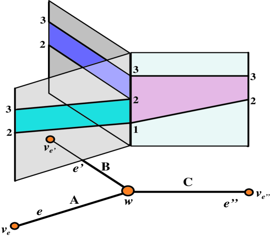
Figure 6. Constructing the surface $X(G,\alpha)$ in the vicinity of a trivalent vertex $w\in G$. The verticies $v_{e},v_{e^{\prime}},v_{e^{\prime\prime}}\in\beta G$ are the centers of edges $e,e^{\prime},e^{\prime\prime}$ of $G$.

Proof.

Let $\mathsf{A},\mathsf{B},\mathsf{C}$ denote the three distinct colors, and $\mathcal{P}=\{\mathsf{A},\mathsf{B},\mathsf{C}\}$ the entire pallet.

Consider a $2$-dimensional space $Z=G\times(0,4)$. It has singularities in the form of binders of the-page open books (see Fig.1.6 ). The binders correspond to the verticies of $G$.

First, employing a given coloring $\alpha$, we will construct a piecewise linear surface $\hat{X}(G,\alpha)\subset Z$. The vector field on $\hat{X}(G,\alpha)$ will be induced by the product structure in $Z$.

For each edge $e\subset G$ and its barycenter $v_{e}\in\beta G$, we place the interval $v_{e}\times[2,3]\subset Z$ over $v_{e}$. Let $\hat{e}$ be half of the interval $e\subset G$, bounded two vericies $v_{e}\in\beta G$ and $w\in G$. Over $\hat{e}$, we place a strip $E\subset Z$; its construction depends on the color attached to the interval $[v_{e},w]$ as follows:

• if the color of $[v_{e}w]$ is $\mathsf{A}$, then we link the vertex $v_{e}\times 2$ with the vertex $w\times 1$ by a line in the rectangle $R=[v_{e},w]\times(0,4)$, and the vertex $v_{e}\times 3$ with the vertex $w\times 2$ by another line in $R$;

• if the color of $[v_{e},w]$ is $\mathsf{B}$, then we link by a line in $R$ the vertex $v_{e}\times 2$ with the vertex $w\times 2$, and the vertex $v_{e}\times 3$ with the vertex $w\times 3$ by another line;

• if the color of $[v_{e},w]$ is $\mathsf{C}$, then we link by a line in $R$ the vertex $v_{e}\times 2$ with the vertex $w\times 1$, and the vertex $v_{e}\times 3$ with the vertex $3\times w$ by another line.

By definition, $E(e,w)$ is the strip in $[v_{e},w]\times(0,4)$, bounded by the two lines whose construction is has been described above. Thanks to the monotonicity of the bijections $A:\{2,3\}\to\{1,2,3\}$, $B:\{2,3\}\to\{1,2,3\}$, and $C:\{2,3\}\to\{1,2,3\}$ that correspond to the colors $\mathsf{A},\mathsf{B},\mathsf{C}$, the lines that bound the strips $E(e,w)$ do not intersect. We denote by $\hat{X}(G,\alpha)$ the union of all such strips.

The local model of each binder implies that indeed $\hat{X}(G,\alpha)$ is piecewise linear surface, imbedded in the singular space $Z$. Inside $Z$, one can smoothen the sharp edges of the boundary $\partial\hat{X}(G,\alpha)$ in order to get a smooth surface $X(G,\alpha)$ (can you visualize this smoothing in the vicinity of point $w\times 2$ from Fig. 6?). The restriction of the product structure in $Z$ to its subspace $X(G,\alpha)$ produces a smooth non-vanishing vector field $v(G,\alpha)$ on $X(G,\alpha)$. Its trajectories (the vertical lines in $Z$) will be simply tangent to $\partial X(G,\alpha)$ exactly at the points of the type $2\times w$, where $w$ runs over the set of verticies of $G$. By Theorem 4.1, this field $v(G,\alpha)$ is of the gradient type.

Conversely, any traversally generic and concave vector field $v$ on a connected compact surface $X$ with boundary, produces a map $\Gamma:X\to\mathcal{T}(v)$, where the space of trajectories is a finite trivalent graph. Its verticies are in 1-to-1 correspondence with the points of the locus $\partial_{2}^{+}X(v)$.

As a point $v_{e}$ in the open edge $e$ of the graph $\mathcal{T}(v)$ approaches a vertex $w$, the intersection of the $v$-trajectory $\gamma=\Gamma^{-1}(v_{e})$ with the boundary $\partial X$ defines a bijection of the $v$-ordered set $\gamma\cap\partial X$ of cardinality $2$ to a $v$-ordered set $\Gamma^{-1}(w)\cap\partial X$ of cardinality $3$, the orders being respected by the bijections. This determines one of three colors we attach to the half-edge $[v_{e},w]$. Therefore the geometry of the flow determines a tricoloring of the graph $\beta\mathcal{T}(v)$. ∎

The next theorem answers Questions 6.1 and 6.2.

Theorem 6.2.

• For any orientable connected surface $X$ with boundary, the two complexities are equal: $gc^{+}(X)=c^{+}(X)$. Moreover, any such $X$, but the disk, admits a boundary concave traversally generic vector field. As a result, for any orientable connected $X$ with boundary, but the disk, the two complexities are equal to $-2\chi(X)$.

• For any non-orientable connected surface $X$ with boundary, which is a boundary connected sum of several punctured Klein bottles and annuli, $gc^{+}(X)=c^{+}(X)=-2\chi(X)$ as well. Again, any such $X$ admits a boundary concave traversally generic vector field.

• In contrast, the Möbius band $M^{\circ}$ does not admit a boundary concave traversally generic vector field. In fact, $c^{+}(M^{\circ})=0$ and $gc^{+}(M^{\circ})=1$.

• Moreover, $c^{+}(M^{\circ}\#_{\partial}X)\leq c^{+}(X)+2$ and $gc^{+}(M^{\circ}\#_{\partial}X)\leq gc^{+}(X)+3$ for any $X$ as in the first two bullets.

Proof.

Consider the boundary connected sum $X_{1}\#_{\partial}X_{2}$ of two compact surfaces $X_{1}$ and $X_{2}$. The Euler number of the sum satisfies the rule

$$\chi(X_{1}\#_{\partial}X_{2})=\chi(X_{1})+\chi(X_{2})-1.$$

On the other hand, given two boundary generic fields $v_{1}$ and $v_{2}$, there exists a traversally generic field $w$ on $X_{1}\#_{\partial}X_{2}$ such that

$$|\partial_{2}^{+}(X_{1}\#_{\partial}X_{2})(w)|=|\partial_{2}^{+}(X_{1})(v_{1})|+|\partial_{2}^{+}(X_{2})(v_{2})|+2.$$

Indeed, we may attach a $1$-handle $H$ to $\partial_{1}^{-}X_{1}(v_{1})\coprod\partial_{1}^{+}X_{2}(v_{2})$ so that an $H$ has a neck with respect to the extension $w$. Such field $w$ contributes two points to $\partial_{2}^{+}(X_{1}\#_{\partial}X_{2})(w)$. Of course, this construction fails when $\partial_{1}^{-}X_{1}(v_{1})\coprod\partial_{1}^{+}X_{2}(v_{2})=\emptyset$; however, for traversing fields $v$, both loci $\partial_{1}^{\pm}X(v)\neq\emptyset$.

By Corollary 4.1, if $X$ admits a boundary concave field, then $c^{+}(X)=-2\chi(X)$, provided $\chi(X)\leq 0$. In particular, if $X$ with a non-positive Euler number admits a boundary concave traversally generic $v$, then

$$gc^{+}(X)=c^{+}(X)=-2\chi(X).$$

Let $v_{1}$ and $v_{2}$ be some boundary generic/ traversally generic fields which deliver the two gradient complexities. The previous arguments about extending $v_{1}$ and $v_{2}$ across the handle $H$ imply that if $gc^{+}(X_{1})=-2\chi(X_{1})$ and $gc^{+}(X_{2})=-2\chi(X_{2})$ (say both surfaces admit boundary concave and traversally generic fields), then

$$gc^{+}(X_{1}\#_{\partial}X_{2})\leq gc^{+}(X_{1})+gc^{+}(X_{2})+2=-2\chi(X_{1}\#_{\partial}X_{2}),$$

provided that $\chi(X_{1}\#_{\partial}X_{2})\leq 0$. Since the reverse inequality holds by Corollary 4.1, we get

$$gc^{+}(X_{1}\#_{\partial}X_{2})=-2\chi(X_{1}\#_{\partial}X_{2})$$

when $gc^{+}(X_{1})=-2\chi(X_{1})$ and $gc^{+}(X_{2})=-2\chi(X_{2})$.

Recall the topological classification of closed connected surfaces. Any such surface is either a sphere, or a connected sum of several tori (the orientable case), or a connected sum of several projective spaces (the non-orientable case). Therefore any connected surface with boundary is obtained from the surfaces in this list by deleting at least one disk.

Let $T^{\circ}$ denote the complement to an open disk in a $2$-torus, and $M^{\circ}$ denote the complement to an open disk in a projective plane—the Möbius band—, and let $A$ denote the annulus. Thus any connected surface with boundary is either a disk $D$, or a boundary connected sum of several copies of punctured tori $T^{\circ}$ and annuli $A$ (the orientable case), or a boundary connected sum of several copies of Möbius bands $M^{\circ}$ and annuli $A$ (the non-orientable case).

Let us now compute the complexities of the basic blocks in this decomposition. Note that $c^{+}(D)=0=gc^{+}(D)$, since $D$ admits a convex traversing flow. Also $c^{+}(A)=0=gc^{+}(A)$, the latter equality being delivered by the radial gradient field.

We claim that $c^{+}(T^{\circ})=2=gc^{+}(T^{\circ})$. Indeed, since $\chi(T^{\circ})=-1$, by Corollary 4.1, we get $c^{+}(T^{\circ})\geq 2$. On the other hand, there exists a trivalent graph $G_{T}$ with an appropriate tricoloring and exactly two verticies such that, applying the construction from Theorem 6.1, we produce a traversally generic field $v(G_{T},\alpha)$ on the surface $X(G_{T},\alpha)=T^{\circ}$ with the cardinality $2$ locus $\partial_{2}^{+}X(G_{T},\alpha)(v(G_{T},\alpha))$. As a result, both complexities of $T^{\circ}$ equal to $2$.

Similar considerations apply to the punctured Klein bottle $K^{\circ}=M^{\circ}\#_{\partial}M^{\circ}$ and a different trivalent graph $G_{K}$ with two verticies and an appropriate tricoloring. Since $\chi(K^{\circ})=-1$, we conclude that $c^{+}(K^{\circ})=2=gc^{+}(K^{\circ})$.

The third trivalent graph $G_{A}$ with two verticies and an appropriate tricoloring delivers a traversally generic boundary concave flow on a punctured annulus $A^{\circ}$, the disk with two holes. Thus, $c^{+}(A^{\circ})=2=gc^{+}(A^{\circ})$.

In fact, Theorem 6.1 implies that $T^{\circ},K^{\circ},A^{\circ}$ are the only connected surfaces of the gradient complexity $2$ that admit concave traversally generic fields. Indeed, just start with the tree “$>\bullet-\bullet<$” with two trivalent verticies and consider the ways one can identify its four leaves in pairs. Then consider all admissible tricologings of the resulting graphs $G$. This cases will deliver the three model tricolored graphs $G_{T},G_{K},G_{A}$.

Now the “quasi-additivity” of Euler numbers and gradient complexities under the connected sum operations imply that the gradient complexity of boundary connected sums

$$X=(T^{\circ}\#_{\partial}\dots\#_{\partial}T^{\circ})\#_{\partial}(A\#_{\partial}\dots\#_{\partial}A)\#_{\partial}(K^{\circ}\#_{\partial}\dots\#_{\partial}K^{\circ})$$

of several copies of the model surfaces $T^{\circ},K^{\circ},A$ is equal to $2|\chi(X)|$. Indeed, these properties imply that $gc^{+}(X)\leq 2\cdot|\chi(X)|$, while in general $gc^{+}(X)\geq 2\cdot|\chi(X)|$. Moreover, every such surface $X$ admits a boundary concave traversally generic field (by the $1$-handle-with-a-neck argument), since the basic blocks $T^{\circ},K^{\circ}$ and $A$ do.

The Möbius band $M^{\circ}$ is different. We notice that $M^{\circ}$ admits a non-vanishing vector field $v$ with a single closed trajectory—the core of the Möbius band—and transversal to the boundary $\partial M^{\circ}$. Thus, $c^{+}(M^{\circ})=0$. Now consider a trivalent graph $G_{M}$ with a single vertex of valency $3$ and a single vertex of valency $1$ (this $G_{M}$ is a circle to which a radius is attached). The construction from Theorem 6.1 applies to produce a remarkable embedding of the Möbius band in the product $G_{M}\times[0,4]$. So we conclude that $M^{\circ}$ admits a traversally generic field $v$ (not concave!) with $\partial_{2}^{+}X(v)$ being a singleton ($\partial_{2}^{-}X(v)$ is a singleton as well). As a result, $gc^{+}(M^{\circ})\leq 1$. On the other hand, any traversally generic field $v$ on $M^{\circ}$ must produce the graph $\mathcal{T}(v)$ which is homotopy equivalent to a circle, the homotopy type of $M^{\circ}$. If $gc^{+}(v)=0$, this graph $\mathcal{T}(v)$ has no trivalent verticies, in which case, $\mathcal{T}(v)$ is homeomorphic to a circle. So $M^{\circ}\to\mathcal{T}(v)$ must be a fibration whose fibers (the $v$-trajectories) are segments. Moreover, thanks to the field $v$, this fibration is orientable, a contradiction with the non-orientability of $M^{\circ}$. Therefore, we conclude that $gc^{+}(M^{\circ})=1$, while $c^{+}(M^{\circ})=0$.

Finally, for any $X$ which is a boundary connected sum of $T^{\circ}$’s, $K^{\circ}$’s, and $A$’s, by the same arguments, the inequalities $c^{+}(M^{\circ}\#_{\partial}X)\leq-2\chi(X)+2$ and $gc^{+}(M^{\circ}\#_{\partial}X)\leq-2\chi(X)+3$ hold. This validates the claim in the last bullet. ∎

7. Combinatorics of tangency for traversing flows in 2D

Pick an extension $\hat{X}$ of a given compact surface $X$ by adding an external collar to $X$. Let $\hat{v}$ be an extension of a given field $v$ into $\hat{X}$. Pick a smooth auxiliary function $z:\hat{X}\to\mathbb{R}$ such that:

• $0$ is a regular value of $z$,

• $z^{-1}(0)=\partial X$,

• $z^{-1}((-\infty,0])=X$,

Definition 7.1.

Let $\hat{\gamma}$ be a $\hat{v}$-trajectory through a point $x\in\partial X$. We say that $\hat{\gamma}$ has the order/multiplicity of tangency $k$ to $\partial X$ at $x$, if $\mathcal{L}_{\hat{v}}^{\{j\}}(z)=0$ for all $j<k$, and $\mathcal{L}_{\hat{v}}^{\{k\}}(z)\neq 0$ at $x$ . Here $\mathcal{L}_{\hat{v}}^{\{j\}}(z)$ denotes the $j^{th}$ iterated $\hat{v}$-directional derivative of the function $z$. $\diamondsuit$

Given a traversally generic vector field $v$ on a compact connected surface $X$, we will attach the combinatorial pattern $(1,1)$ to a typical $v$-trajectory $\gamma\subset X$ that corresponds to the edges of the graph $\mathcal{T}(v)$, the pattern $(121)$ to the trajectories that correspond to the trivalent verticies of $\mathcal{T}(v)$, and the pattern $(2)$ to the univalent verticies (see Fig. 4). In fact, the numbers 1 and 2 in these patterns reflect the order of tangency of the curves $\hat{\gamma}$ and $\partial X$ at the points of $\gamma\cap\partial X$ (see Definition 7.1). On a given compact surface $X$, for traversally generic fields $v$ no other patterns (say, like $(1221)$ or $(13)$) occur. In $2D$, this conclusion follows from Definition 7.1.

The lemma below is another way to state this fact. Its proof, relying on the Malgrange Preparation Theorem [Mal], can be found in [K2].

Lemma 7.1.

Let $v$ be a traversally generic field on $X$. Extend $(X,v)$ to a pair $(\hat{X},\hat{v})$. In the vicinity of each $v$-trajectory $\gamma$, there exist special local coordinates $(u,x)$ in $\hat{X}$ and a real polynomial $P(u,x)$ of degree $2$ or $4$ such that:

• each $\hat{v}$-trajectory is given by the equation $\{x=const\}$,

• the boundary $\partial X$ is given by the polynomial equation $\{P(u,x)=0\}$,

• $X$ is given by the polynomial inequality $\{P(u,x)\leq 0\}$.

The polynomial $P(u,x)$ takes three canonical forms:

1. $u(u-1)$, which corresponds to the combinatorial pattern $\mathbf{(11)}$,

2. $u^{2}-x,$ which corresponds to the combinatorial pattern $\mathbf{(2)}$,

3. $u\big{(}(u-1)^{2}+x\big{)}(u-2),$ which corresponds to the pattern $\mathbf{(121)}$. $\diamondsuit$

To summarize, at $\partial_{2}X(v)$ the order of tangency is $2$; the trajectories through $\partial_{2}^{+}X(v)$ have the combinatorial tangency pattern $(121)$, and through $\partial_{2}^{-}X(v)$ the combinatorial tangency pattern $(2)$. The rest of trajectories have the pattern $(11)$.

We denote by $\Omega^{\bullet}_{{}^{\prime}\langle 1]}$ the partially ordered set whose elements are $(11),(2),(121)$ and the order is defined by $(11)\succ(2)$ and $(11)\succ(121)$. This combinatorics does not look impressive. However, in higher dimensions, traversally generic fields on $(n+1)$-manifolds with boundary generate a rich and interesting partially ordered finite list $\Omega^{\bullet}_{{}^{\prime}\langle n]}$ of combinatorial tangency patters. The poset $\Omega^{\bullet}_{{}^{\prime}\langle n]}$ is universal in each dimension $n+1$. They are discussed in [K3].

8. Holography of traversing flows on surfaces

Let $v$ be a traversing and boundary generic vector field on a compact connected surface $X$ with boundary. For any point $z\in\partial_{1}^{+}X(v)$, consider the closest point $w(z)\in\partial_{1}^{-}X(v)$ that can be reached by moving along the trajectory $\gamma_{z}$ through $z$ in the direction of $v$ (see Fig. 7). Note that $w(z)=z$ if and only if $z\in\partial_{2}^{-}X(v)$.

The correspondence $z\to w(z)$ defines a map

$$C_{v}:\partial_{1}^{+}X(v)\to\partial_{1}^{-}X(v)$$

which we call the causality map. It is a distant relative of the classical Poincaré Return Map.

Alternatively, one can think of $C_{v}$ as determining a partial order “$z\prec w(z)$” among the points of the boundary $\partial X$.

The word “causality” in the name of $C_{v}$ is motivated by the following pivotal special case.

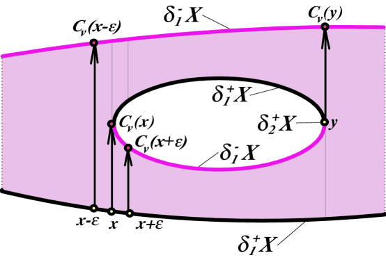
Figure 7. An example of the causality map $C_{v}:\partial_{1}^{+}X(v)\to\partial_{1}^{-}X(v)$. Note the discontinuity of $C_{v}$ in the vicinity of $x$.

Example 8.1. Let $w=w(\theta,t)$ be a smooth time-dependent vector field on the circle $S^{1}$ (equipped with the angular coordinate $\theta$). It gives rise to a vector field $v=(w,1)$ on the cylinder $S^{1}\times\mathbb{R}$. We think about the factor $S^{1}$ as space and about the factor $\mathbb{R}$ as time $t$. So we call $S^{1}\times\mathbb{R}$ the space of events. Note that $v\neq 0$ is a gradient-like field with respect to the time function $T:S^{1}\times\mathbb{R}\to\mathbb{R}$.

Pick any smooth compact and connected surface $X\subset S^{1}\times\mathbb{R}$. Such a surface has a boundary $\partial X$. We call $X$ the event domain, and its boundary $\partial X$ the event horizon.

Since the field $v\neq 0$ is traversing in $X$, the map $C_{v}$ is well-defined. Then the map $C_{v}:\partial_{1}^{+}X(v)\to\partial_{1}^{-}X(v)$ indeed gives rise the causality relation on the event horizon: the correspondence $C_{v}$ reflects the evolution of an event $z$ into the event $C_{v}(z)$. $\diamondsuit$

Let $\mathcal{C}(\partial_{2}^{+}X(v))$ denotes the union of $v$-trajectories through the points of the concavity locus $\partial_{2}^{+}X(v)$.

The causality map is discontinuous at the points of the intersection $\mathcal{C}(\partial_{2}^{+}X(v))\cap\partial_{1}^{+}X(v)$ (see Fig. 7). On the positive side, the discontinuities of the causality map $C_{v}$ are not too bad: in a sense, the map has “left” and “right” limits.

Given a pair $(X,v)$, the $v$-trajectories, viewed as unparametrized $v$-oriented curves, produce an oriented $1$-dimensional foliation $\mathcal{F}(v)$ on $X$.

Theorem 8.1.

(The Causal Holography Principle in 2D).

Let $(X_{1},v_{1})$ and $(X_{2},v_{2})$ be two compact connected surfaces with boundaries, carrying traversally generic vector fields $v_{1}$ and $v_{2}$, respectively. Assume that there is a diffeomorphism $\Phi^{\partial}:\partial X_{1}\to\partial X_{2}$ which conjugates the two causality maps:

$$C_{v_{2}}\circ\Phi^{\partial}=\Phi^{\partial}\circ C_{v_{1}}.$$

Then $\Phi^{\partial}$ extends to a diffeomorphism $\Phi:X_{1}\to X_{2}$ which maps the oriented foliation $\mathcal{F}(v_{1})$ to the oriented foliation $\mathcal{F}(v_{2})$.

Proof.

We will only sketch the argument. A fully developed proof of the multidimensional analogue of this theorem is contained in [K4].

First, we notice that since $C_{v_{1}}$ and $C_{v_{2}}$ are $\Phi^{\partial}$-conjugate, the diffeomorphism $\Phi^{\partial}$ induces a well-defined continuous map $\Phi_{\mathcal{T}}:\mathcal{T}(v_{1})\to\mathcal{T}(v_{2})$ of the trajectory spaces. Moreover, $\Phi_{\mathcal{T}}$ preserves the stratifications of the two trajectory spaces/graphs by the combinatorial type of trajectories. That is, the trivalent verticies of $\mathcal{T}(v_{1})$ are mapped to the trivalent verticies of $\mathcal{T}(v_{2})$, the univalent verticies are mapped to univalent verticies, and the interior of the edges to the interior of the edges.

Then we pick a smooth function $f_{2}:X_{2}\to\mathbb{R}$ such that $df_{2}(v_{2})>0$. With the help of $\Phi^{\partial}$, we pull-back $f_{2}|_{\partial X_{2}}$ to get a smooth function $f_{1}^{\partial}:\partial X_{1}\to\mathbb{R}$ such that

$$f_{1}^{\partial}(z)<f_{1}^{\partial}(C_{v_{1}}(z))$$

for all $z\in\partial_{1}^{+}X_{1}(v_{1})$.

Then we argue that $f_{1}^{\partial}$ extends to a smooth function $f_{1}$ such that $df_{1}(v_{1})>0$.

We use $f_{1}$ to embed $X_{1}$ in the product $\mathcal{T}(v_{1})\times\mathbb{R}$ by the formula

$$\alpha_{(v_{1},f_{1})}(z)=(\gamma_{z},f_{1}(z)),$$

where $\gamma_{z}$, the $v_{1}$-trajectory through $z$, is viewed as the point $\Gamma_{1}(z)$ of the graph $\mathcal{T}(v_{1})$. Similarly, we use $f_{2}$ to embed the surface $X_{2}$ in the product $\mathcal{T}(v_{2})\times\mathbb{R}$ with the help of the map $\alpha_{(v_{2},f_{2})}$.

Finally, we employ $\Phi_{\mathcal{T}}$, $f_{1}$ and $f_{2}$ to construct a map

$$\hat{\Phi}:\mathcal{T}(v_{1})\times\mathbb{R}\to\mathcal{T}(v_{2})\times\mathbb{R}$$

by the formula

$$\hat{\Phi}(\gamma,t)=\big{(}\Phi_{\mathcal{T}}(\gamma),\,f_{1}(f_{2}^{-1}(t))\big{)},$$

where $t$ belongs to the $f_{2}$-image of the trajectory $\Gamma_{2}^{-1}\big{(}\Phi_{\mathcal{T}}(\gamma)\big{)}$.

Crudely, the restriction of $\hat{\Phi}$ to $\alpha_{v_{1},f_{1}}(X_{1})\subset\mathcal{T}(v_{1})\times\mathbb{R}$ is the desired diffeomorphism $\Phi:X_{1}\to X_{2}$.

Note that, in general, the pull-back $\Phi^{\ast}(f_{2})$ is not $f_{1}$; so the parametrizations of the trajectories are not respected by the diffeomorphism $\Phi$, but the $1$-foliations $\mathcal{F}(v_{1})$ and $\mathcal{F}(v_{2})$ are. ∎

Corollary 8.1.

Let $X$ be a compact connected surface with boundary, and $v$ a smooth traversally generic vector field on it.

Then the knowledge of the causality map $C_{v}:\partial_{1}^{+}X(v)\to\partial_{1}^{-}X(v)$ is sufficient for a reconstruction of the pair $(X,\mathcal{F}(v))$, up to a diffeomorphism that is constant on $\partial X$. $\diamondsuit$

The world “holography” is present in the name of Theorem 8.1 since the surface $X$ and the $2D$-dynamics of the $v$-flow in it are recorded on two $1$-dimensional screens, $\partial_{1}^{+}X(v)$ and $\partial_{1}^{-}X(v)$.

Theorem 8.1 and Corollary 8.1 are valid in any dimension ([K4]).

Example 8.2. Let $v$ be a traversally generic field on a connected surface $X$ whose boundary $\partial X$ is a single loop. Then the boundary $\partial X$ is divided into $q$ disjoint arcs $a_{1},\dots,a_{q}$ that form $\partial_{1}^{+}X(v)$ and $q$ complementary arcs $b_{1},\dots,b_{q}$ that form $\partial_{1}^{-}X(v)$. The causality map

$$C_{v}:\coprod_{i=1}^{q}a_{i}\to\coprod_{i=1}^{q}b_{i}$$

can be represented by its graph $G(C_{v})\subset\prod_{i,j}a_{i}\times b_{j}$.

The map $C_{v}$ (the curve $G(C_{v})$) is discontinuous at exactly $c^{+}(v)$ points in $\coprod_{i=1}^{q}a_{i}$ that correspond to the points of the intersection $\mathcal{C}(\partial_{2}^{+}X(v))\cap\partial_{1}^{+}X(v)$. There the map $C_{v}$ has distinct left and right limits.

According to the Corollary 8.1, the curve $G(C_{v})\subset\prod_{i,j}a_{i}\times b_{j}$ determines $X$ and the un-parametrized dynamic of the $v$-flow, up to a diffeomorphism $\Phi:X\to X$ that is the identity on $\partial X$. Note that the number $q$ alone is not sufficient even to determine the genus of the surface $X$. $\diamondsuit$

Revisiting Example 8.2, we get the following interpretation of Corollary 8.1:

Corollary 8.2.

For any smooth time-dependent vector field $w$ on the circle $S^{1}$, the causality relation on the event horizon $\partial X$ is sufficient for a reconstruction of the event domain $X$ and the un-parametrized dynamics of the $(w,1)$-flow, up to a diffeomorphism of $X$ that is the identity on $\partial X$. $\diamondsuit$

The theory of billiards on Riemmanian surfaces $X$ with boundary benefits from applying the $3D$-version of the Causal Holography to the geodesic flow on the $3$-fold $SX$, the space of unit tangent vectors on $X$. See [K4] for some of these applications. In addition to geodesic billiards, they include the classic inverse geodesic scattering problems.

9. Convex quasi-envelops and characteristic classes of traversing flows on orientable surfaces

Traversing flows have interesting characteristic classes—elements of certain cohomology—associated with them. In dimension two, they are quite primitive, but for high-dimensional flows, surprisingly rich (see [K6]).

We have seen that the traversally generic flows exhibit a very particular combinatorial patterns of tangency to the boundary $\partial X$. In particular, for generic $2D$-flows, no tangencies of orders $\geq 3$ occur.

There is a nice link between this behavior and the spaces of smooth functions $f:\mathbb{R}\to\mathbb{R}$ or even polynomials that have no zeros of multiplicities $\geq 3$. To explain the connection, we will need the following definition/construction.

Let $\mathcal{F}$ denote the space (in the $C^{\infty}$-topology) of smooths functions $f:\mathbb{R}\to\mathbb{R}$ which are identically $1$ outside of a compact set. Let $\mathcal{F}_{\leq 2}$ be its subspace, formed by functions that have zeros only of multiplicity $\leq 2$.

Such spaces of functions with “moderate singularities” have been studied in depth by V. I. Arnold [Ar] and V. A. Vassiliev [V]. In $2D$, we employ just a tiny portion of their results. The main theorem of Arnold-Vassiliev describes the weak homotopy/homology types of the spaces $\mathcal{F}_{\leq k}$ for all $k\geq 2$. In particular, the homology of the space $\mathcal{F}_{\leq 2}$ is isomorphic to the homology of $\Omega S^{2}$, the space of loops on a $2$-sphere ([V])! Arnold proved also that the fundamental group $\pi_{1}(\mathcal{F}_{\leq 2})\approx\mathbb{Z}$ [Ar].

For an even non-negative integer $d$, we will also explore the subspaces $\mathcal{F}^{d}_{\leq 2}\subset\mathcal{F}_{\leq 2}$, formed by functions whose degree—the sum of multiplicities of all its zeros—is even and does not exceed $d$.

Let $\hat{v}$ be a boundary convex traversing vector field on an annulus $A$. With the help of $\hat{v}$, we can introduce a product structure $A\approx S^{1}\times[0,1]$ so that the fibers of the projection $A\to S^{1}$ are the $\hat{v}$-trajectories.

Definition 9.1.

Consider a collection $L$ of several smooth immersed loops in the annulus $A$ which intersect and self-intersect transversally and do not have triple intersections.

We say that a boundary convex traversing vector field $\hat{v}$ is generic with respect to $L$, if no $\hat{v}$-trajectory $\gamma$ contains more than one point of self-intersection from $L$ and no more than one point of simple tangency to $L$, but not both. $\diamondsuit$

For a given $L$, by standard techniques of the singularity theory, we can find a perturbation of $\hat{v}$ within the space $\mathcal{V}_{\mathsf{trav}}(A)$ so that the perturbed field is generic with respect to $L$.

Since an immersion is a smooth map of manifolds, whose differential has the trivial kernel, the immersions allow for a transfer of a given vector field on the target manifold to a vector field in the source manifold. The transfer of a non-vanishing field is a non-vanishing field.

All surfaces in this section are orientable. Note that any orientable surface $X$ admits an immersion $\alpha:X\to A$ (or even in the plane $\mathbb{R}^{2}$) (see Fig. 8). We will use this fact to pull-back non-vanishing fields on the target space $A$ to $X$.

Definition 9.2.

Consider an immersion $\alpha:X\to A$ of a given compact orientable surface $X$ into an annulus $A$, equipped with a traversal boundary convex (“radial”) field $\hat{v}$. We call such $\alpha$ generic relative to $\hat{v}$, if $\hat{v}$ is generic with respect to the curves $\alpha(\partial X)$ in the sense of Definition 9.1.

Given a transversally generic field $v$ on a connected compact surface $X$, we call a map $\alpha:(X,v)\to(A,\hat{v})$ a convex quasi-envelop of $(X,v)$ if there exists an immersion $\alpha:X\to A$ which is generic relative to the radial field $\hat{v}$ on $A$, and $v=\alpha^{\ast}(\hat{v})$, the pull-back of $\hat{v}$. $\diamondsuit$

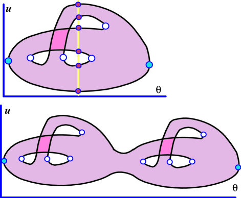
Figure 8. A convex quasi-envelop $\alpha:X\to A$ of a traversally generic field $\alpha^{\ast}(\partial_{u})$ on a punctured torus $X$ (on the top) and on a punctured surface $X$ of genus $2$ (on the bottom). In both examples, the cardinality of the $\theta$-fibers $\leq 6$.

Given a boundary generic relative to $\hat{v}$ immersion $\alpha:X\to A$, the $\alpha$-pullback (transfer) of the field $\hat{v}$ defines a vector field $v\neq 0$ on $X$. Since $\alpha$ is an immersion, evidently the pull-back $v$ is traversing on $X$. Moreover, $v$ is taversally generic in the sense of Definition 5.2, since no $v$-trajectory $\gamma$ has more than one point of simple tangency to $\partial X$.

Definition 9.3.

Let $\alpha:X\to A$ be a regular embedding of a given compact surface $X$ into an annulus $A$, carrying a traversal boundary convex field $\hat{v}$. We denote by $v$ the pull-back of $\hat{v}$ under $\alpha$. If $\alpha$ is traversally generic relative to $\hat{v}$, then we say that the pair $(A,\hat{v})$ is a convex envelop of $(X,v)$.

$\diamondsuit$

The existence of a convex envelop puts significant restrictions of the topology of $X$: such orientable surfaces $X$ do not have $1$-handles. In other words, they are disks with holes.

Lemma 9.1.

If a compact connected surface $X$ with boundary has a pair of loops whose transversal intersection is a singleton, then no traversal flow on $X$ admits a convex envelop. In other words, if a connected surface $X$ with boundary has a handle, then no traversal flow on $X$ can be convexly enveloped.

Proof.

By Lemma 1.2, the space $\hat{X}$ of a convex envelop is either a disk or an annulus, both surfaces residing in the plane. No two loops in the plane intersect transversally at a singleton. Thus, for surfaces with a handle, no convex envelops exist. ∎

So the existence of a convex envelop severally restricts the topology of surface $X$. To incorporate surfaces with handles into our constructions, we have introduced the notion of a convex quasi-envelop (Definition 9.2).

Now we are in position to explore a connection between immersions $\alpha:(X,v)\subset(A,\hat{v})$ of a given surface $X$ in the annulus $A$, such that $v=\alpha^{\ast}(\hat{v})$ and $\hat{v}$ is generic with respect to $\alpha(\partial X)$ on one hand, and loops in the functional spaces $\mathcal{F}_{\leq 2}$ on the other.

Let $\alpha(\partial X)^{\times}$ denote the set of self-intersections of the curves forming the image $\alpha(\partial X)$. Let $\alpha(\partial X)^{\circ}$ denote the set $\alpha(\partial X)\setminus\alpha(\partial X)^{\times}$.

With the pattern $\alpha(\partial X)$ we associate an auxiliary smooth function $z_{\alpha}:A\to\mathbb{R}$, subject to the following properties:

• $z_{\alpha}^{-1}(0)=\alpha(\partial X)$,

• $0$ is the regular value of $z_{\alpha}$ at the points of $\alpha(\partial X)^{\circ}$,

• in the vicinity of each point $a\in\alpha(\partial X)^{\times}$, consider local coordinates $(x_{1},x_{2})$ such that $\{x_{1}=0\}$ and $\{x_{2}=0\}$ define the two intersecting branches of $\alpha(\partial X)$; then locally $z_{\alpha}=c\cdot x_{1}x_{2}$, where the constant $c\neq 0$.

• $z_{\alpha}=1$ in the vicinity of $\partial A$,

• the sign of $z_{\alpha}$ changes to opposite as a path crosses an arc from $\alpha(\partial X)^{\circ}$ transversally.

Here we denote by $A^{\circ}$ the interior of the annulus $A$. Let $\phi:A^{\circ}\to\mathbb{R}$ be a smooth function so that $d\phi(\hat{v})>0$ in $A^{\circ}$ and $\phi(\hat{\gamma}\cap A^{\circ})=\mathbb{R}$ for all $\hat{v}$–trajectories $\hat{\gamma}$ in $A$. Then, with the help of $z_{\alpha}$ and $\phi$, we get a map $J_{z_{\alpha}}:\mathcal{T}(\hat{v})\to\mathcal{F}_{\leq 2}$ whose target is the space of smooth functions $f:\mathbb{R}\to\mathbb{R}$ with no zeros of multiplicity $\geq 3$ and that are identically $1$ outside of a compact set in $\mathbb{R}$. We define the map $J_{z_{\alpha}}$ by the formula

(9.2) $$J_{z_{\alpha}}(\hat{\gamma})=(z_{\alpha}|_{\hat{\gamma}})\circ(\phi|_{\hat{\gamma}})^{-1},$$

where, abusing notations, $\hat{\gamma}$ stands for both a $\hat{v}$-trajectory in $A$ and for the corresponding point in the trajectory space $\mathcal{T}(\hat{v})\approx S^{1}$.

For a fixed $\alpha$, it is easy to check that the homotopy class $[J_{z_{\alpha}}]$ of $J_{z_{\alpha}}$ does not depend on the choice of the auxiliary function $z_{\alpha}$, subject to the five properties in (LABEL:eq1.7) (the space of such $z_{\alpha}$’s is convex and thus contractible).

We pick a generator $\kappa\in\pi_{1}(\mathcal{F}_{\leq 2})\approx\mathbb{Z}$ (see [Ar]) and define the integer $J^{\alpha}$ by the formula $J^{\alpha}\cdot\kappa=[J_{z_{\alpha}}]$. As a result, any immersion $\alpha:X\to A$, which is generic with respect to $\hat{v}$, produces a homotopy class $[J_{z_{\alpha}}]\in\pi_{1}(\mathcal{F}_{\leq 2})$ and an integer $J^{\alpha}$.

The isomorphism $\pi_{1}(\mathcal{F}_{\leq 2})\approx\mathbb{Z}$ follows from the work of V. I. Arnold [Ar] by a slight modification of his arguments, which we will describe next (see Theorem 9.1). The main difference between our constructions and the ones from [Ar] is that Arnold uses the critical loci of functions from $\mathcal{F}_{\leq 2}$, while we are using the zero loci.

Generic loops in $\beta:S^{1}\to\mathcal{F}_{\leq 2}$ have an interpretation in terms of finite collections $C$ of smooth closed curves in the annulus $A$ with no inflection points with respect to their tangent lines of the form $\{\theta=const\}$ in the $(u,\theta)$-coordinates. We call such tangent lines $\theta$-vertical. Furthermore, the generic homotopy between such loops $\beta$ correspond to some cobordism relation between the corresponding plane curves, the cobordism also avoids the $\theta$-vertical inflections.

First, let us spell out the genericity requirements on the collections $C$ of closed curves in the annulus $A$:

1. $C\subset A$ is a finite collectionof closed smooth immersed curves $\{C_{j}\}_{j}$,

2. the projections $\{\theta:C_{j}\to S^{1}\}_{j}$ have Morse type singularities only,

3. the self-intersections and mutual intersections of the curves $\{C_{j}\}_{j}$ are transversal and no triple intersections are permited,

4. at each double intersection, the two banches of $C$ are not parallel to the $u$-coordinate,

5. the $\theta$-images of the intersections and of the critical values of $\{\theta:C_{j}\to S^{1}\}_{j}$ are all distinct in $S^{1}$,

6. the cardinality of each fiber of $\theta:C\to S^{1}$ does not exceed a given natural number $d$.

Definition 9.4.

Given two collections $C_{0}$ and $C_{1}$ of immersed closed curves as in (LABEL:eq1.9), we say that they are cobordant with no $\theta$-vertical inflections, if there is a smooth function $F:A\times[0,1]\to\mathbb{R}$ such that:

• $0$ is a regular value of $F$,

• the restriction of the projection $T:A\times[0,1]\to[0,1]$ to the zero set $W=_{\mathsf{def}}F^{-1}(0)$ is a Morse function,

• $C_{0}=W\cap(A\times\{0\})$ and $C_{1}=W\cap(A\times\{1\})$,

• for each $t\in[0,1]$, the section $C_{t}=_{\mathsf{def}}W\cap(A\times\{t\})$ is such that $C_{t}$ has no $\theta$-horizontal inflections

• for each $t\in[0,1]$ the cardinality of the fibers of $\theta:C_{t}\to S^{1}$ does not exceed a given natural number $d$. $\diamondsuit$

It is possible to verify that the cobordism with no $\theta$-vertical inflections is an equivalence relation among collections of curves as in (LABEL:eq1.9). Indeed, if $C$ is cobordant to $C^{\prime}$ with the help of $F$, and $C^{\prime}$ to $C^{\prime\prime}$ with the help of $F^{\prime}$, then there exists a piecewise smooth function $F\cup F^{\prime}:A\times[0,2]\to\mathbb{R}$ whose restriction to $A\times[0,1]$ is $F$ and to $A\times[1,2]$ is a $(+1)$-shift of $F^{\prime}$. Smoothing $F\cup F^{\prime}$ along $A\times\{1\}$ in the normal direction and scaling down the interval $[0,2]$ to $[0,1]$, produces the desired function-cobordism $F\ast F^{\prime}:A\times[0,1]\to\mathbb{R}$.

So we can talk about the set of bordisms $\mathbf{B}_{\mathsf{no\,\theta-inflect.}}$, based on collections of closed curves in the annulus with no $\theta$-vertical inflections. This set is a group: the operation $C,C^{\prime}\Rightarrow C\ast C^{\prime}$ is defined by the union $\tilde{C}\cup\tilde{C}^{\prime}\subset A$, where $\tilde{C}\subset S^{1}\times(0,0.5)$ and $\tilde{C}^{\prime}\subset S^{1}\times(0.5,1)$ are the images of $C$ and $C^{\prime}$, scaled down in the $u$-direction by the factor $0.5$ and placed in sub-annuli of $A=S^{1}\times[0,1]$. The role of $-C$ is played by the mirror image of $C$ with respect to a vertical (equivalently, horizontal) line, a fiber of $\theta:A\to S^{1}$.

Note that this operation $\ast$ may affect the maximal cardinalities $d$ and $d^{\prime}$ of the fibers $\theta:C\to S^{1}$ and $\theta:C^{\prime}\to S^{1}$ in a somewhat unpredictable way. In any case, the fiber cardinality of $\theta:C\ast C^{\prime}\to S^{1}$ has the upper boundary $d+d^{\prime}$.

The previous constructions deliver the following proposition, a slight modification of Theorem from [Ar].

Theorem 9.1.

The fundamental group $\pi_{1}(\mathcal{F}_{\leq 2})$ is isomorphic to the bordism group $\mathbf{B}_{\mathsf{no\,\theta-inflect.}}$, based on finite collections of immersed loops with no $\theta$-vertical inflections in the annulus $A$ and subject to the constraints (LABEL:eq1.9). The isomorphism is induced by the correspondence

$$K:\{\beta:S^{1}\to\mathcal{F}_{\leq 2}\}\Rightarrow\{\beta(\theta)^{-1}(0)\}_{\theta\in[0,2\pi]}\subset A.$$

$\diamondsuit$

This theorem is a foundation of a graphic calculus that converts homotopies of loops in the functional space $\mathcal{F}_{\leq 2}$ into cobordisms of closed loop patterns in the annulus $A$ with no $\theta$-vertical inflections.

Figures 10 - 14 show an application of this calculus. They explain why any loop in $\mathcal{F}_{\leq 2}$ is homotopic to an integral multiple of a generator $\kappa\in\pi_{1}(\mathcal{F}_{\leq 2})$, represented by a model loop pattern $K\subset A$ as in Fig. 9, diagram (a) or (b).

We orient the annulus $A=S^{1}\times[0,1]$ so that the the $\theta$-coordinate, corresponding to $S^{1}$, is the first, and the $u$-coordinate, corresponding to $[0,1]$, is the second.

We fix an orientation of $X$, thus picking orientations for each component of $\partial X$. Given an orientation-preserving immersion $\alpha:(X,v)\subset(A,\hat{v})$ such that $\alpha(\partial X)$ has the properties as in (LABEL:eq1.9), we notice that the polarity of $a\in\partial_{2}^{+}X(v)$ is $\oplus$ if and only if $\alpha_{\ast}(\nu_{a})$, where $\nu_{a}$ is the inner normal to $\partial X$ at $a$, points in the direction of $\theta$. Otherwise, the polarity of $a$ is $\ominus$ (see Fig. 9).

Theorem 9.2.

Any orientation-preserving immersion $\alpha:(X,v)\subset(A,\hat{v})$ such that $\hat{v}$ is generic with respect to $\alpha(\partial X)$ produces a map $J_{z_{\alpha}}:S^{1}\to\mathcal{F}_{\leq 2}$ (see (9.2)). Its homotopy class $[J_{z_{\alpha}}]=J^{\alpha}\cdot\kappa$, where $\kappa$ denots a generator of $\pi_{1}(\mathcal{F}_{\leq 2})\approx\mathbb{Z}$.

The integer $J^{\alpha}$ can be computed by the formula:

$$J^{\alpha}=\#\{\partial_{2}^{+,\oplus}X(v)\}-\#\{\partial_{2}^{+,\ominus}X(v)\}$$

and thus does not depend on $\alpha$ (as long as the transfer $\alpha^{\ast}(\hat{v})=v$).

Moreover, $|J^{\alpha}|\leq c_{2}^{+}(v)$, the complexity of the $v$-flow.

Proof.

Let $d=_{\mathsf{def}}\max_{\hat{\gamma}}\#\{\hat{\gamma}\cap\alpha(\partial X)\}$ be the maximal cardinality of the intersections of the $\hat{v}$-trajectories $\hat{\gamma}$ with the loops’ pattern $\alpha(\partial X)$. Since $X$ bounds $\partial X$, $d$ is even.

For any $\hat{v}$-generic immersion $\alpha:X\subset A$, we pick an auxiliary function $z_{\alpha}:A\to\mathbb{R}$, adjusted to $\alpha$ as in (LABEL:eq1.9). By the previous arguments, this choice produces the loop $J_{z_{\alpha}}:S^{1}\to\mathcal{F}^{d}_{\leq 2}$. Although the loop $J_{z_{\alpha}}$ is generated by an immersion $\alpha:X\to A$, in the process of deforming $J_{z_{\alpha}}$ by a cobordism $F:A\times[0,1]\to\mathbb{R}$ with no $\theta$-vertical inflections as in Definition 9.4, we may destroy this connection with the original $\alpha$: the new curve patterns $\{C_{t}\}_{t\in[0,1]}$ in $A$ may not be produced by immersions $\{\alpha_{t}:X\to A\}_{t\in[0,1]}$.

Let us describe an algorithm (see Figures 10 - 14) that reduces a given pattern $C_{0}=J_{z_{\alpha}}^{-1}(0)\subset A$ to a pattern from the canonical set of patterns $\{n\cdot K\}_{n\in\mathbb{Z}}$ (as in Fig. 9) by a cobordism $F:A\times[0,1]\to\mathbb{R}$. We will perform a sequence of elementary surgeries on the set $C_{0}$, executed inside of the cylindrical shell $A\times[0,1]$. It is sufficient to construct a smooth surface $W\subset A\times[0,1]$ as in Definition 9.4, for which $W\cap A\times\{0\}=C$ and $W\cap A\times\{1\}=J^{\alpha}\cdot K$; then one can define a function $F:A\times[0,1]\to\mathbb{R}$, appropriately adjusted to $W$, so that $0$ is a regular value of $F$ and $F^{-1}(0)=W$.

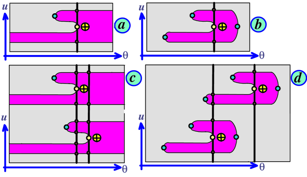
Figure 9. Two equivalent representations of a generator $\kappa\in\pi_{1}(\mathcal{F}_{\leq 2})$ (diagrams (a) and (b)). Diagrams (c) and (d) portray $2\kappa$. Note the polariity $\oplus$ of the tangent $\hat{v}$-trajectories with the combinatorial pattern $(\dots 121\dots)$. A mirrow image of these shapes with respect to a vertical line delivers $-\kappa$ and $-2\kappa$.

As we modify the $t$-section $C_{t}\subset A\times\{t\}$, we keep track of the checker board polarities $+,-$, attached to the regions of $A\setminus C_{t}$; through the process, the polarity of the region adjacent to $\partial A$ remains “$+$”. Let us denote by $A_{t}^{-}$ the region of the negative polarity that is “bounded” by the curve pattern $C_{t}\subset A\times\{t\}$. $A_{t}^{+}$ denotes the complementary set. Informally, the regions of polarity $+$ are the regions where the function $F$ from Definition 9.4 is non-negative.

With the help of this polarization $\{A_{t}^{+},A_{t}^{-}\}$ of the annulus $A$, the points $a\in\partial_{2}(C_{t},\hat{v})$, where $\hat{v}$-flow is tangent to $C_{t}$, acquire the polarization “$+$” or “$-$”: if the germ of the trajectory $\hat{\gamma}_{a}$ is contained in $A_{t}^{-}$, then the polarity of $a$ is defined to be “$+$”, otherwise it is “$-$”. Moreover, if the inner normal $\nu_{a}$ to the region $A^{-}_{t}$ at $a$ has the same direction as the coordinate $\theta$ on $A$, then the second polarity of $a$ is defined to be “$\oplus$”, otherwise it is “$\ominus$”. As a result, we can talk about the four sets: $\partial_{2}^{+,\oplus}(A_{t}^{-},\hat{v})$, $\partial_{2}^{+,\ominus}(A_{t}^{-},\hat{v})$, $\partial_{2}^{-,\oplus}(A_{t}^{-},\hat{v})$, $\partial_{2}^{-,\ominus}(A_{t}^{-},\hat{v})$. We simplify the notations for these loci as: $\partial_{2}^{+,\oplus}C_{t},\;\partial_{2}^{+,\ominus}C_{t},\;\partial_{2}^{-,\oplus}C_{t},\;\partial_{2}^{-,\ominus}C_{t}.$

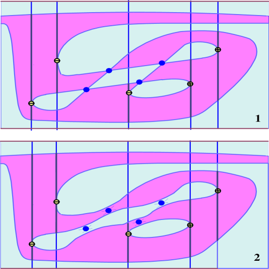
Figure 10. An immersion $\alpha$ of a surface $X$—the torus with two holes—in an annulus $A$ (represented as a rectangle with the two vertical sides to be glued). The points whose $\alpha$-fiber has cardinality $2$ form a unshaded parallelogram (diagram 1). Eliminating crossings of $\alpha(\partial X)$ by $1$-surgery (diagram 2).

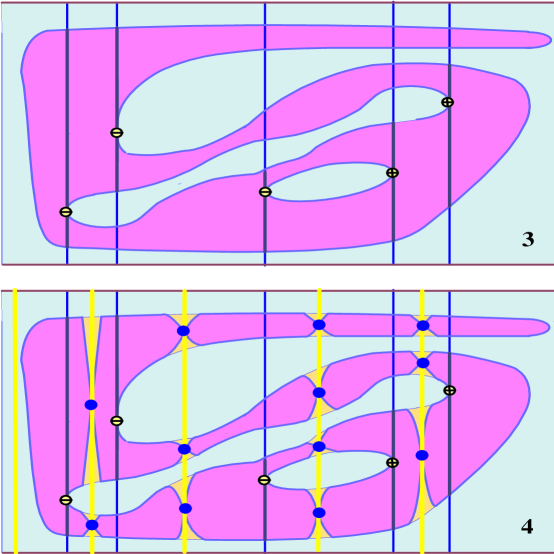
Figure 11. $1$-surgery on $A_{t}^{+}$ places the curve pattern $C_{t}$ in a rectangle (diagram 3). In preparation for the next step, new crossings are introduced momentarily so that they reside in the $\theta$-fibers that separate the trajectories through the set $\partial_{2}^{+}C_{t}$ (diagram 4).

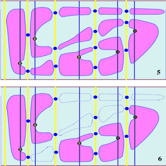
Figure 12. Further $1$-surgery on $A_{t}^{-}$ breaks the curves from $C_{t}$ in groups, confined to $\theta$-vertical strips, so that each strip contains a single point from $\partial_{2}^{+}C_{t}$ (diagram 5). Then the disks with no points from $\partial_{2}^{+}C_{t}$ are eliminated by $2$-surgery on $A_{t}^{+}$ (diagram 6).

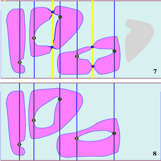
Figure 13. In preparation for cancellation of trajectories of the opposite second polarity, the regions of $A_{t}^{-}$ are moved by an isotopy which preserves the fibers of $\theta:A\to S^{1}$ (the isotopy is not required by our $7$ step algorithm; it is applied only to decrease the number of figures), and the new crossings are created momentarily (diagram 7). Completing the $1$-surgery places each pair of trajectories of the opposite second polarity in an annulus, a portion of $A_{t}^{-}$.

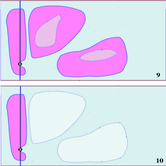
Figure 14. Performing $2$-surgeries on the inner circles of the annuli in Fig. 13 converts $A_{t}^{-}$ into a disjoint union of disks, each disk containing a single trajectory of the same second polarity $\{\oplus,\ominus\}$ at most (diagram 10). Further $0$-surgery eliminates the disks without points of the first polarity $+$ (diagram 10). This leaves only the disks with a single point of the first polarity $+$ and a common second polarity ($\ominus$ in this example, so that $J^{\alpha}=-1$ for the $\alpha$ in Fig. 10).

Let us describe an algorithm that constructs a cobordism with no $\theta$-vertical inflextions between a given loop pattern $\alpha(\partial X)$ and a few copies of the canonical pattern as in Fig. 9.

(1) At any stage of this construction, we can resolve each crossing $a\in(C_{t})^{\times}$ in a preferred way. The two branches of the preferred resolution will be transversal to the $\theta$-fiber through $a$. When the vector $\hat{v}(a)$ points inside $A_{t}^{-}$, the resolution will add a 1-handle to $A_{t}^{+}$, when the vector $\hat{v}(a)$ points inside $A_{t}^{+}$, the resolution will add a 1-handle to $A_{t}^{-}$. In any case, the sets $\partial_{2}^{+,\oplus}C_{t}$, $\partial_{2}^{+,\ominus}C_{t}$ are not affected. As a result of these resolutions, the new pattern $C^{\prime}_{t}\subset A$ is a disjoint union of simple smooth curves with no $\theta$-vertical inflections. Moreover, it shares with $C_{0}$ the same sets $\partial_{2}^{+,\oplus}\sim$, $\partial_{2}^{+,\ominus}\sim$ (see Fig. 10).

(2) Next we will pick and fix one regular value $\theta_{\star}\in S^{1}$ of the map $\theta:C_{t}\to S^{1}$. The intersection of $\theta^{-1}\cap A_{t}^{+}$ consists of several intervals. By performing $1$-surgery of $C_{t}$ along each of these intervals we get a new loop pattern $C^{\prime}_{t}$ which has an empty intersection with the $\theta$-fiber over the point $\theta_{\star}$. Moreover no $\theta$-vertical inflections were introduced in the process. The original loci $\partial_{2}^{+,\oplus}\sim$, $\partial_{2}^{+,\ominus}\sim$ are preserved (while the loci $\partial_{2}^{-,\oplus}\sim$, $\partial_{2}^{-,\ominus}\sim$ are changed). Therefore we may assume that $C_{t}=C^{\prime}_{t}$ is contained in a rectangle $R\subset A$ and $C_{t}$ shares the numbers of points from the loci $\partial_{2}^{+,\oplus}\sim$, $\partial_{2}^{+,\ominus}\sim$ with the original $C_{0}$ (see Fig. 11, diagram 3).

(3) Consider the set $\Theta^{+}_{t}\subset S^{1}$ of critical values of $\theta:C_{t}\to S^{1}$ for the critical points from $\partial_{2}^{+}C_{t}$. We pick a regular value $\theta^{\sharp}_{i}$ in-between each pair of adjacent critical values $\theta_{i},\theta_{i+1}\in\Theta^{+}_{t}$. Then we apply $1$-surgery on $A_{t}^{+}$ as in (2) to empty the region $A_{t}^{-}$ in the vicinity of the fiber $\theta^{-1}(\theta_{i}^{\sharp})$ (see Fig. 11, diagram 4).

(4) As a result of these surgeries, $A_{t}^{-}$ turns into a disjoint union of connected regions, each of which contains a single point of the set $\partial_{2}^{+}(C_{t})$ at most (see Fig. 12, diagram 5).

(5) By Lemma 4.1, any connected region of $A_{t}^{-}\subset R\subset A$ with no points from $\partial_{2}^{+}\sim$ is a disk. It can be eliminated by a $0$-surgery (see Fig. 12, diagram 6).

(6) Pairs of points $a\in\partial_{2}^{+,\oplus}\sim$ and $b\in\partial_{2}^{+,\ominus}\sim$ can be cancelled via a surgery on their regions $D_{a},D_{b}\subset A_{t}^{-}$ (as shown in Fig. 13, diagrams 7 and 8, and Fig. 14, diagrams 9 and 10). This cancellation of pairs will be executed gradually and with some care.

Any strip $S_{i}\subset A$, bounded by the vertical lines $\{\theta=\theta^{\sharp}_{i}\}$ and $\{\theta=\theta^{\sharp}_{i+1}\}$, contains a single region $D_{a}$ with $a\in\partial_{2}^{+}C_{t}$. If the points of opposite second polarity ($\oplus,\ominus$) exist, then there are two adjacent vertical strips $S_{i},S_{i+1}$ such that $a_{i}\in S_{i}\cap\partial_{2}^{+,\oplus}C_{t}$ and $b_{i}\in S_{i+1}\cap\partial_{2}^{+,\oplus}C_{t}$ have opposite second polarities. We attach to $D_{a_{i}}\coprod D_{b_{i}}$ two $1$-handles to form an annulus $A_{a_{i}b_{i}}$ as in Figures 12 and 13. To complete the cancellation of opposite pairs, we perform $2$-surgery on the inner circles of the annuli $\{A_{a_{i}b_{i}}\}$. This converts the annuli into disks, residing in $A_{t}^{-}$. They can be eliminated by $0$-surgery along the outer circles of $\{A_{a_{i}b_{i}}\}$’s (see Fig. 14, diagram 10).

It may happen that the model domain $D_{a_{i}}$ as in Fig. 9, (b), and “its mirror image” $D_{b_{i}}$ with respect to a vertical line $\{\theta=\theta_{i}^{\sharp}\}$ are positioned so that their horns are pointing in opposite directions. In such a case, they can be cancelled by a slightly different sequence of elementary surgeries (see [Ar]). Alternatively, taking a trip around the annulus $A$, we will find a pair of adjacent strips such that their domains $D_{a}$ and $D_{b}$ of opposite second polarity can “lock horns”. For them, the previous recipe will apply.

This cancellation procedure can be repeated by considering the remaining adjacent pairs of regions with the opposite second polarity untill no regions with the opposite second polarity are left.

(7) As a result of all these steps, $A^{-}_{t}$ is either empty, or a disjoint union of disks (as in Fig. 9), each of which contains a single point from $\partial_{2}^{+}\sim$ (and tree points from $\partial_{2}^{-}\sim$); the second polarities of such points are the same for all disks. Thus we got an integral multiple of the basic pattern as in Fig. 9 and proved that $\pi_{1}(\mathcal{F}_{\leq 2})\approx\mathbb{Z}$.

Note that the original difference $\#\{\partial_{2}^{+,\oplus}X(v)\}-\#\{\partial_{2}^{+,\ominus}X(v)\}$ between the numbers of $\hat{v}$-trajectories with polarities $\oplus$ and $\ominus$ and of the combinatorial types $(\dots 121\dots)$ is preserved under the modifications in (1)-(7).

The original maximal cardinality $d$ of the $\theta$-fibers evidently does not increase under the steps (1)-(7).

Finally, we notice that

$$c^{+}(v)=_{\mathsf{def}}\#\{\partial_{2}^{+,\oplus}(v)\}+\#\{\partial_{2}^{+,\ominus}(v)\}$$

$$\geq\quad|\#\{\partial_{2}^{+,\oplus}(v)\}-\#\{\partial_{2}^{+,\ominus}(v)\}|.$$

∎

Remark 9.1. It is interesting and somewhat surprising to notice that the invariant $J^{\alpha}=\#\{\partial_{2}^{+,\oplus}(v)\}-\#\{\partial_{2}^{+,\ominus}(v)\}$ reflects more the topology of the field $v=\alpha^{\ast}(\hat{v})$ than the topology of the surface $X$: in fact, any integral value of $J^{\alpha}$ can be realized by a traversally generic field $v$ on a disk $D$ which even admits a convex envelop! A portion of the boundary $\partial D$ looks like a snake with respect to the field $\hat{v}$ of the envelop. For any $X$, the effect of deforming a portion of $\partial X$ into a snake is equivalent to adding several times a spike (an edge and a pair of univalent and trivalent verticies) to the graph $\mathcal{T}(v)$. Evidently, these operations do not affect $H_{1}(\mathcal{T}(v);\mathbb{Z})\approx H_{1}(X;\mathbb{Z})$.

In contrast, $\#\{\partial_{2}^{+,\oplus}(v)\}+\#\{\partial_{2}^{+,\ominus}(v)\}\geq 2|\chi(X)|$ has a topological significance for $X$.

For example, for $\alpha$ as in Fig. 8, $J^{\alpha}=0$. If we subject $\alpha$ to an isotopy that introduces a snake-like pattern of Fig. 9, (a), then for the new immersion $\alpha^{\prime}$, the invariant $J^{\alpha^{\prime}}=1$. $\diamondsuit$

Remark 9.2. Consider a connected oriented surface $X$ with a connected boundary. It is a boundary connected sum of a few copies of $T^{\circ}$, the torus with a hole. A punctured torus admits an immersion $\alpha:T^{\circ}\to A$ in the annulus so that the cardinality of the fibers of $\theta:\alpha(\partial T^{\circ})\to S^{1}$ does not exceed $6$ (see Fig. 8). Therefore, any connected oriented surface $X$ with boundary admits an immersion $\alpha:X\to A$ with the property $\#\{\theta^{-1}(\theta_{\star})\cap\alpha(\partial X)\}\leq 6$ for all $\theta_{\star}\in S^{1}$. $\diamondsuit$

Let us glance at the implications of Theorems 9.1 and 9.2 and give them a new, perhaps, more natural spin.

The finite-dimensional space $\mathcal{P}^{d}_{\leq 2}$ of real monic polynomials of an even degree $d$ and with no real roots of multiplicity $\geq 3$ is a natural “approximation” of the functional space $\mathcal{F}^{d}_{\leq 2}$. Of course, a polynomial from $\mathcal{P}^{d}_{\leq 2}$ is not a function from $\mathcal{F}_{\leq 2}$: it is not identically $1$ outside of a compact set. However, there is an embedding $\mathcal{I}_{d}:\mathcal{P}^{d}_{\leq 2}\to\mathcal{F}_{\leq 2}$ that, in the vicinity of $\pm\infty$, “levels down to $1$” any real polynomial $P$ of an even degree $d$. Its image belongs to the subspace $\mathcal{F}^{d}_{\leq 2}$. This embedding is described by an analytic formula (see [V]) as follows. Fix an auxiliary smooth function $\chi:\mathbb{R}\to[0,1]$ such that $\chi(u)=0$ for $|u|\leq 1$, $\chi(u)=1$ for $|u|\geq 2$, and $\partial\chi/\partial u\neq 0$ for $1<|u|<2$. Let $\mu(P)$ denote the sum of absolute values of the coefficients of the monic $P$. Then

$$\mathcal{I}_{d}(P)(u)=_{\mathsf{def}}P(u)+(1-P(u))\cdot\chi(u/\mu(p)).$$

In fact, the zeros of any polynomial $P$ are in 1-to-1 correspondence with the zeros of the function $\mathcal{I}_{d}(P)$ and their multiplicities are preserved.

Consider the “forbidden set” $\mathcal{F}^{d}_{\geq 3}\subset\mathcal{F}^{d}$ of functions $f$ that have at least one zero of multiplicity $\geq 3$. Among them, the functions $f$ that have exactly one zero of multiplicity $3$ form an open and dense subset $(\mathcal{F}^{d}_{\geq 3})^{\circ}$.

For each $f\in(\mathcal{F}^{d}_{\geq 3})^{\circ}$, let $u^{\star}_{f}$ be the unique zero of multiplicity $3$.

The set $\mathcal{F}^{d}_{\geq 3}$ has codimension $2$ in $\mathcal{F}^{d}$; so loops in $\mathcal{F}^{d}_{\leq 2}$ may be linked with the locus $\mathcal{F}^{d}_{\geq 3}$ in $\mathcal{F}^{d}$. Here is a model example of such a link (see Fig. 15).

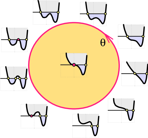
Figure 15. A loop $\big{\{}P(\theta,u)=_{\mathsf{def}}(u-2)[u^{3}+\cos(\theta)u+\sin(\theta)]\big{\}}_{\theta\in[0,2\pi]}$ in the space $\mathcal{P}^{4}_{\leq 2}$, which represents a generator of $\pi_{1}(\mathcal{P}^{4}_{\leq 2})$.

For any $u^{\ast}\in(-2,2)$, consider a $\theta$-family of quartic $u$-polynomials

$$\big{\{}P_{u^{\star}}(u,\theta)=_{\mathsf{def}}(u-2)\big{[}(u-u^{\star})^{3}+\cos(\theta)(u-u^{\star})+\sin(\theta)\big{]}\big{\}}_{\theta\in[0,2\pi]}.$$

Each $P_{u^{\star}}(u,\theta)$ belongs to the space $\mathcal{P}^{4}_{\leq 2}$. The $\mathcal{I}_{4}$-image of this $\theta$-family forms a loop $\{h_{u^{\star}}(u,\theta)\}_{\theta\in[0,2\pi]}$ in $\mathcal{F}^{4}_{\leq 2}$. The loop bounds a $2$-disk

$$D^{2}_{u^{\star}}=_{\mathsf{def}}\big{\{}\mathcal{I}_{4}\big{(}(u-2)[(u-u^{\star})^{3}+x_{1}(u-u^{\star})+x_{0}]\big{)}\big{\}}_{\{x_{0}^{2}+x_{1}^{2}\leq 1\}}$$

in $\mathcal{F}^{4}$, which hits the subspace $\mathcal{F}^{d}_{\geq 3}$ at the singleton $\mathcal{I}_{4}\big{(}(u-2)(u-u^{\star})^{3}\big{)}$.

Similarly, for any $f\in(\mathcal{F}^{d}_{\geq 3})^{\circ}$ and $d\geq 4$, the loop

$$L_{f}=_{\mathsf{def}}\big{\{}f(u,\theta)=h_{u^{\star}_{f}}(u,\theta)\cdot\big{[}f(u)/(u-u^{\star}_{f})^{3}\big{]}\big{\}}_{\theta\in[0,2\pi]}$$

resides in $\mathcal{F}^{d}_{\leq 2}$ and is linked with the component of $(\mathcal{F}^{d}_{\geq 3})^{\circ}$ that contains $f$.

Since the correspondence $f\to u^{\star}_{f}$ is continuous for $f\in(\mathcal{F}^{d}_{\geq 3})^{\circ}$, the homotopy class $[L_{f}]$ of the loop $L_{f}$ does not depend on the choice of $f$ within each component of $(\mathcal{F}^{d}_{\geq 3})^{\circ}$.

In fact, by Theorem 9.2, $[L_{f}]$ is a generator $\kappa$ of $\pi_{1}(\mathcal{F}^{d}_{\leq 2})$. In particular, the $\mathcal{I}_{4}$-image of the loop

$$\big{\{}P(\theta,u)=_{\mathsf{def}}(u-2)[u^{3}+\cos(\theta)u+\sin(\theta)]\big{\}}_{\theta\in[0,2\pi]}$$

in $\mathcal{P}^{4}_{\leq 2}$ is a generator $\kappa$ of $\pi_{1}(\mathcal{F}_{\leq 2})\approx\mathbb{Z}$. Its zero set in the annulus $A=S^{1}\times[-3,3]$ (equipped with the coordinates $(\theta,u)$) is a union of two loops, similar to the ones shown in Fig. 9, (a).

Theorem 11 from [V], makes an important for us claim: the $\mathcal{I}_{d}$-induced map in homology

$$(\mathcal{I}_{d})_{\ast}:H_{j}(\mathcal{P}^{d}_{\leq 2};\,\mathbb{Z})\to H_{j}(\mathcal{F}_{\leq 2};\,\mathbb{Z})$$

is an isomorphism for all $j\leq d/3$. In particular,

$$(\mathcal{I}_{4})_{\ast}:H_{1}(\mathcal{P}^{4}_{\leq 2};\,\mathbb{Z})\to H_{1}(\mathcal{F}_{\leq 2};\,\mathbb{Z})\approx\mathbb{Z}$$

is an isomorphism. Moreover,

$$(\mathcal{I}_{4})_{\ast}:\pi_{1}(\mathcal{P}^{4}_{\leq 2})\to\pi_{1}(\mathcal{F}_{\leq 2})\approx\mathbb{Z}$$

is an isomorphism as well [Ar]. As we proceed, let us keep these facts in mind.

Of course it is much easier to visualize events in the $4$-dimensional space $\mathcal{P}^{4}_{\leq 2}$ than their analogues in the infinite-dimensional $\mathcal{F}^{4}_{\leq 2}$. This will be our next task. It will lead us to explore the beautiful stratified geometry of the Swallow Tail discriminant surface.

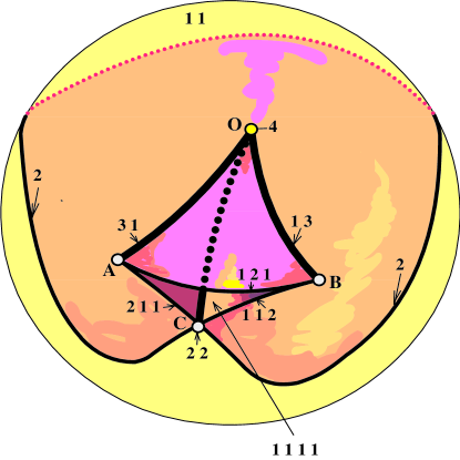
Figure 16. The Swallow Tail Singularity is the critical locus of the Whitney projection of the hypersurface $\{P(u,x_{0},x_{1},x_{2})=u^{4}+x_{2}u^{2}+x_{1}u+x_{0}=0\}$ onto the space $\mathbb{R}_{\mathsf{coef}}^{3}$ with the coordinates $(x_{0},x_{1},x_{2})$. The strata in $\mathbb{R}_{\mathsf{coef}}^{3}$ are indexed by combinatorial types of real divisors of the polynomial $P(u,\sim)$: (1111), (11), $\emptyset$; (211), (121), (112); (22), (13), (31); (4). They divide the target space into three 3-cells, four 2-cells, three 1-cells, and one 0-cell.

Consider the subspace $\tilde{\mathcal{P}}^{4}_{\leq 2}\subset\mathcal{P}^{4}_{\leq 2}$, formed by the monic depressed polynomials $P(u)$. Since $\tilde{\mathcal{P}}^{4}_{\leq 2}$ is a deformation retract of $\mathcal{P}^{4}_{\leq 2}$ ([Ar]), these two are homotopy equivalent. So it is a bit easier to visualize the generator $\tilde{\kappa}\in\pi_{1}(\tilde{\mathcal{P}}^{4}_{\leq 2})$ (rather than $\kappa\in\pi_{1}(\mathcal{P}^{4}_{\leq 2})$), since $\tilde{\mathcal{P}}^{4}_{\leq 2}$ is a domain in $\mathbb{R}_{\mathsf{coef}}^{3}$, the space of the coefficients $x_{0},x_{1},x_{2}$.

The polynomials with real roots of multiplicity $\geq 2$ form a singular surface $H\subset\mathbb{R}_{\mathsf{coef}}^{3}$, the famous Swallow Tail (see Fig. 16). The point-polynomial $u^{4}$ (the strongest singularity $O$ of $H$), together with the polynomials that have one root of multiplicity $3$, must be excluded from $\mathbb{R}_{\mathsf{coef}}^{3}$ to form $\tilde{\mathcal{P}}^{4}_{\leq 2}$. These excluded polynomials form two branches of a curve $\mathcal{C}\subset H$, whose apex $O$ is the origin and whose branches extend to infinity. One branch $OB$ of $\mathcal{C}$ correspond to polynomials with the smaller simple root followed by the root of multiplicity $3$; the other branch $OA$ of $\mathcal{C}$ correspond to polynomials with the smaller root of multiplicity $3$, followed by the simple root. The curve $OC$, the self-intersection locus of $H$, represents polynomials with two distinct roots of multiplicity $2$. It belongs to the set $\tilde{\mathcal{P}}^{4}_{\leq 2}$ .

Thus $\pi_{1}(\tilde{\mathcal{P}}^{4}_{\leq 2})=\pi_{1}(\mathbb{R}_{\mathsf{coef}}^{3}\setminus\mathcal{C})\approx\mathbb{Z}$. Therefore the generator $\tilde{\kappa}\in\pi_{1}(\tilde{\mathcal{P}}^{4}_{\leq 2})$ is represented by an oriented loop in $\mathbb{R}_{\mathsf{coef}}^{3}$ that winds once around the curve $\mathcal{C}$. Such loop $\tilde{\kappa}$ must hit once the locus $H_{(121)}\subset H$, formed by polynomials whose real zeros conform to the pattern $(121)$: indeed, the curve $\mathcal{C}=OA\cup OB\cup O$ is the boundary of the surface $H_{(121)}$.

Traversing $H_{(121)}$ from the chamber of polynomials with $4$ real roots to the chamber of polynomials with $2$ real roots picks a normal to $H_{(121)}$ orientation. Similar rule of orientation can be applied to the stratum $H_{(112)}$ bounded by the curves $OC\cup OB$, the stratum $H_{(211)}$ bounded by the curves $OC\cup OA$, and the stratum $H_{(2)}$ that separates the chamber with two real roots from the chamber with no real roots at all.

For any smooth loop $\beta:S^{1}\to\tilde{\mathcal{P}}^{4}_{\leq 2}$ which is in general position to $H$ and its strata, consider the zero set

$$\Delta(\beta)=_{\mathsf{def}}\{(\theta,u)|\;\beta(\theta)(u)=0\}\subset S^{1}\times\mathbb{R}.$$

Thanks to the very definition of the target space $\tilde{\mathcal{P}}^{4}_{\leq 2}$, the set $\Delta(\beta)$ is a collection of closed curves with transversal self-intersections, no triple intersections, no self-tangencies, and no $\theta$-vertical inflections. The cardinality of the fiber of $\theta:\Delta(\beta)\to S^{1}$ does not exceed $4$.

Now the linking number $J^{\beta}=_{\mathsf{def}}\mathsf{lk}(\beta(S^{1}),\mathcal{C})$ equals the algebraic intersection of the loop $\beta(S^{1})$ with the surface $H_{(121)}$ that bounds $\mathcal{C}$. Each time the loop $\beta(S^{1})$ intersects the surface $H_{(121)}$ transversally in the direction of the positive normal, a point from $\partial_{2}^{+,\oplus}\Delta(\beta)$ is generated, and each time $\beta(S^{1})$ intersects $H_{(121)}$ is in the direction of the negative normal, a point from $\partial_{2}^{+,\ominus}\Delta(\beta)$ is generated. In particular, the generator $\kappa:S^{1}\to\tilde{\mathcal{P}}^{4}_{\leq 2}$ of $\pi_{1}(\tilde{\mathcal{P}}^{4}_{\leq 2})$ has the property $\mathsf{lk}(\beta(S^{1}),\mathcal{C})=1$. Therefore we get

$$\mathsf{lk}(\beta(S^{1}),\mathcal{C})=\beta(S^{1})\circ H_{(121)}=\#\{\partial_{2}^{+,\oplus}\Delta(\beta)\}-\#\{\partial_{2}^{+,\ominus}\Delta(\beta)\},$$

the baby model of the formula from Theorem 9.2. This number is an invariant of the homotopy class of the loop $\beta$.

Similarly, each time the loop $\beta(S^{1})$ intersects the surface $H_{(2)}$ transversally in the direction of the positive normal, a point from $\partial_{2}^{-,\oplus}\Delta(\beta)$ is generated, and each time $\beta(S^{1})$ intersects $H_{(2)}$ is in the direction of the negative normal, a point from $\partial_{2}^{-,\ominus}\Delta(\beta)$ is generated.

Note that perhaps not any set $\Delta(\beta)$ is the image $\alpha(\partial X)$ of an immersion $\alpha:X\to S^{1}\times\mathbb{R}$ for some orientable surface $X$. But the generator $\kappa$ in Fig. 9, (a), is. Also, if we insist that the cardinality of the $\theta$-fibers $\leq 4$, we cannot accommodate surfaces $X$ with handles. According to Remark 9.2, to accommodate them, we need to deal with polynomials/functions of degree $6$ at least.

Let us describe briefly how this “degree $6$ polynomial model” works. We will see that the increasingly complex combinatorics of tangency begins to play a significant role.

To simplify the notations, we identify $\mathcal{P}^{6}$ with its image $\mathcal{I}_{6}(\mathcal{P}^{6})\subset\mathcal{F}^{6}$ and the cylinder $S^{1}\times\mathbb{R}$ with the interior of the annulus $A$.

The combinatorial patterns $\omega$ of real divisors of monic degree $6$ real polynomials are numerous:

• (111111), (1111), (11), $\emptyset$;

• (21111), (12111), (11211), (11121), (11112), (211), (121), (112), (2);

• (2211), (1221), (1122), (2121), (2112), (1212),   (22);

• (3111), (1311), (1131), (1113), (31), (13);

• etc.

We denote by $\mathcal{P}^{6}_{\omega}$ the set of real monic polynomials whose real divisors conform to the combinatorial pattern $\omega=(\omega_{1},\omega_{2},\dots,\omega_{s})$, where $\{\omega_{i}\}_{1\leq i\leq s}$ are natural numbers. We denote by $|\omega|$ the $l_{1}$-norm of the vector $\omega$. Evidently, $|\omega|\leq 6$.

The sets $\{\mathcal{P}^{6}_{\omega}\}_{\omega}$ form a partition of the space $\mathcal{P}^{6}$. In fact, each $\mathcal{P}^{6}_{\omega}$ is homeomorphic to an open ball of dimension $6-|\omega|^{\prime}$, where $|\omega|^{\prime}=|\omega|-s$ ([K3]). The closure $\bar{\mathcal{P}}^{6}_{\omega}$ of $\mathcal{P}^{6}_{\omega}$ in $\mathbb{R}^{6}_{\mathsf{coef}}$ is an affine semi-algebraic variety. By resolving $\bar{\mathcal{P}}^{6}_{\omega}$ appropriately, one can show that the partition $\{\mathcal{P}^{6}_{\omega}\}_{\omega}$ defines a structure of a $CW$-complex on $\mathcal{P}^{6}$, or rather, on its one-point compactification ([K3]). So we may think of $\mathcal{P}^{6}_{\omega}$’s as being “cells” (although $\bar{\mathcal{P}}^{6}_{\omega}$ may not be homeomorphic to an infinite cone over a closed ball).

Let $H\subset\mathcal{P}^{6}$ denote the set of monic polynomials with multiple roots, the $5$-dimensional discriminant variety. The first bullet lists the four $6$-dimensional chambers-cells in which $H$ divides $\mathcal{P}^{6}$. The second bullet lists all $5$-dimensional strata in which $H$ is divided by the strata of dimension $4$. The first three bullets list the monic polynomials that form the space $\mathcal{P}^{6}_{\leq 2}$. The third and the fourth bullets list the $4$-dimensional cells-strata. The forbidden locus $\mathcal{P}^{6}_{\geq 3}$ is the union of strata, labeled by the combinatorial types in the fourth bullet and on. Then $\mathcal{P}^{6}_{\geq 3}$ is the closure of the set

$$\mathcal{P}^{6}_{(3111)}\cup\mathcal{P}^{6}_{(1311)}\cup\mathcal{P}^{6}_{(1131)}\cup\mathcal{P}^{6}_{(1113)}\cup\mathcal{P}^{6}_{(31)}\cup\mathcal{P}^{6}_{(13)}.$$

We can orient each cell $\mathcal{P}^{6}_{\omega}$ so that

$$\partial\bar{\mathcal{P}}^{6}_{(12111)}=\bar{\mathcal{P}}^{6}_{(3111)}-\bar{\mathcal{P}}^{6}_{(1311)}+\bar{\mathcal{P}}^{6}_{(1221)}-\bar{\mathcal{P}}^{6}_{(1212)},$$

$$\partial\bar{\mathcal{P}}^{6}_{(11121)}=\bar{\mathcal{P}}^{6}_{(1131)}-\bar{\mathcal{P}}^{6}_{(1113)}+\bar{\mathcal{P}}^{6}_{(2121)}-\bar{\mathcal{P}}^{6}_{(1221)},$$

$$\partial\bar{\mathcal{P}}^{6}_{(121)}=\bar{\mathcal{P}}^{6}_{(31)}-\bar{\mathcal{P}}^{6}_{(13)}+\bar{\mathcal{P}}^{6}_{(2121)}-\bar{\mathcal{P}}^{6}_{(1212)}.$$

The operator $\partial$ in these formulas should be understood in the spirit of algebraic topology as the boundary operator on cellular chains (and not as a topological boundary of the appropriate sets) [K6].

Adding the three formulas above, we get that the forbidden set, viewed as a $4$-chain, is an algebraic boundary of a $5$-chain:

$$\mathcal{P}^{6}_{\geq 3}=_{\mathsf{def}}\,\bar{\mathcal{P}}^{6}_{(3111)}-\bar{\mathcal{P}}^{6}_{(1311)}+\bar{\mathcal{P}}^{6}_{(1131)}-\bar{\mathcal{P}}^{6}_{(1113)}+\bar{\mathcal{P}}^{6}_{(31)}-\bar{\mathcal{P}}^{6}_{(13)}$$

$$=\partial\big{(}\bar{\mathcal{P}}^{6}_{(12111)}+\bar{\mathcal{P}}^{6}_{(11121)}+\bar{\mathcal{P}}^{6}_{(121)}\big{)}.$$

Now consider a smooth loop $\beta:S^{1}\to\mathcal{P}^{6}_{\leq 2}$. By a small perturbation we may assume that $\beta(S^{1})$ is transversal to the hypersurfaces $\mathcal{P}^{6}_{(12111)},\mathcal{P}^{6}_{(11121)},\mathcal{P}^{6}_{(121)}$ that bound the cycle $\bar{\mathcal{P}}^{6}_{\geq 3}$. Therefore

$$\mathsf{lk}\big{(}\beta(S^{1}),\mathcal{P}^{6}_{\geq 3}\big{)}=\beta(S^{1})\circ\big{(}\mathcal{P}^{6}_{(12111)}\cup\mathcal{P}^{6}_{(11121)}\cup\mathcal{P}^{6}_{(121)}\big{)}.$$

Again, we form the set

$$\Delta(\beta)=_{\mathsf{def}}\{(\theta,u)|\;\beta(\theta)(u)=0\}\subset S^{1}\times\mathbb{R}.$$

Then

$$\beta(S^{1})\circ\big{(}\mathcal{P}^{6}_{(12111)}\cup\mathcal{P}^{6}_{(11121)}\cup\mathcal{P}^{6}_{(121)}\big{)}=\#\{\partial_{2}^{+,\oplus}\Delta(\beta)\}-\#\{\partial_{2}^{+,\ominus}\Delta(\beta)\}.$$

Therefore we get

$$\mathsf{lk}\big{(}\beta(S^{1}),\mathcal{P}^{6}_{\geq 3}\big{)}=\#\{\partial_{2}^{+,\oplus}\Delta(\beta)\}-\#\{\partial_{2}^{+,\ominus}\Delta(\beta)\},$$

a version of the formula from Theorem 9.2, being applied to the loop $\beta=J_{z_{\alpha}}$. The loop is produced by a generic with respect to $\hat{v}$ immersion $\alpha:X\to A$, such that the cardinality of the fibers of $\theta:\alpha(\partial X)\to S^{1}$ does not exceed $6$, and by an auxiliary function $z_{\alpha(\partial X)}$.

These considerations are not restricted to polynomials/functions of degree $6$: they apply to any even degree $d$. The application requires a deeper dive into the combinatorics of real polynomial divisors and their modifications, but the spirit is captured by the arguments that deal with degree $6$ (see [K3]).

Any $\hat{v}$-generic immersion $\alpha:X\to A$ also produces a well-defined element $[K_{\alpha}]$ in the set of homotopy classes $[\mathcal{T}(v),\mathcal{F}_{\leq 2}]$ of maps from the trajectory graph $\mathcal{T}(v)$ to the functional space $\mathcal{F}_{\leq 2}$. Its construction is similar to the one of $J_{z(\alpha)}$. Consider the $\hat{v}$-generated obvious map $Q_{\alpha}:\mathcal{T}(v)\to\mathcal{T}(\hat{v})\approx S^{1}$ (each $v$-trajectory is contained in the unique $\hat{v}$-trajectory). Put $K_{\alpha}=_{\mathsf{def}}J_{z(\alpha)}\circ Q_{\alpha}$.

Remark 9.3. Note that, for some immersions $\alpha:X\to A$, the invariant $J^{\alpha}$ may be different from $0$, but $[K_{\alpha}]$ may be trivial. For example, this is the case when $X$ is a disk with a snake-like boundary $\alpha(\partial X)$ with respect to $\hat{v}$. However, there exist immersions $\alpha$ with a nontrivial $[K_{\alpha}]$. For example, such is the immersion in Fig. 10, (1). At the same time, for $\alpha$ in Fig. 11, (3), $[K_{\alpha}]$ is trivial. $\diamondsuit$

Since $\pi_{1}(\mathcal{F}_{\leq 2})\approx\mathbb{Z}$, it follows that $H_{1}(\mathcal{F}_{\leq 2};\mathbb{Z})\approx\mathbb{Z}$. In turn, this implies that the $1$-dimensional cohomology $H^{1}(\mathcal{F}_{\leq 2};\mathbb{Z})\approx\mathbb{Z}$.

Thus $K_{\alpha}$ induces a map

$$K_{\alpha}^{\ast}:H^{1}(\mathcal{F}_{\leq 2};\mathbb{Z})\to H^{1}(\mathcal{T}(v);\mathbb{Z})\approx H^{1}(X;\mathbb{Z}).$$

In particular, we get an element $K_{\alpha}^{\ast}(\kappa^{\ast})\in H^{1}(X;\mathbb{Z})$, where $\kappa^{\ast}$ is a generator of $H^{1}(\mathcal{F}_{\leq 2};\mathbb{Z})\approx\mathbb{Z}$. This cohomology class $K_{\alpha}^{\ast}(\kappa^{\ast})$ is a characteristic class of the given $\hat{v}$-generic immersion $\alpha$.

Theorem 9.1 implies that if two $\hat{v}$-generic immersions $\alpha,\alpha_{1}:X\to A$ are such that the pull-backs $\alpha^{\ast}(\hat{v})=\alpha^{\ast}_{1}(\hat{v})=v$, then $K_{\alpha}^{\ast}(\kappa^{\ast})=K_{\alpha_{1}}^{\ast}(\kappa^{\ast})$. So the cohomology class $K_{\alpha}^{\ast}(\kappa^{\ast})$ is, in fact, a characteristic class of $v$. It is desirable to be able to reach this conclusion without relying on the cobordisms of curves’ patterns in $A$ with no $\theta$-vertical inflections.

Based on the partial evidence, provided by the two polynomial models $\mathcal{P}^{4}_{\leq 2}$ and $\mathcal{P}^{6}_{\leq 2}$, we may conjecture that the value of $K_{\alpha}^{\ast}(\kappa^{\ast})$ on any loop ($1$-cycle) $\delta:S^{1}\to X$ equals to the linking number $\mathsf{lk}(K_{\alpha}(\delta),\mathcal{F}_{\geq 3})$. The validation of this conjecture requires to extend our analysis of the stratified geometry of $\mathcal{P}^{6}_{\leq 2}$ to $\mathcal{P}^{d}_{\leq 2}$ and to show that $\mathcal{I}_{d}:\mathcal{P}^{d}_{\leq 2}\to\mathcal{F}^{d}_{\leq 2}$ is a weak homotopy equivalence for all even $d$. Both steps are realizable with the techniques developed in [K3] and in [K5].

In dimensions higher than two, similar considerations apply to produce characteristic classes of traversally generic flows. They are based on computations of homology of spaces of real monic polynomials with restricted combinatorics of their real divisors. It turns out that the topology of high-dimensional convex envelops is as intricate as the homotopy groups of spheres [K6].

Our investigation of vector flows in Flatland reached its conclusion. To find out how things flow in other lands—“the romances of many dimensions”—([Ab]), the reader could consult with the references below.

References

- [Ab] Abbott, E., Flatland: A Romance of Many Dimensions, Dover Publications, New York, 1992.
- [AK] Alpert, H., Katz, G., Using Simplicial Volume to Count Multi-tangent Trajectories of Traversing Vector Fields, Geometriae Dedicata DOI 10.1007/s10711-015-0104-6 (arXiv:1503.02583v1 [math.DG] (9 Mar 2015)).
- [Ar] Arnold V.I., Spaces of Functions with Moderate Singularities, Func. Analysis & Its Applications, 23(3), 1-10 (1989) (Russ).
- [C] Cohen, R.L., Topics in Morse Theory, Stanford University, 1991.
- [GM] Goresky, M., MacPherson, R., Stratified Morse Theory, Proceedings of Symposia in Pure Mathematics, Vol. 40 (1983), Part 1, 517-533.
- [GM1] Goresky, M., MacPherson, R., Morse theory for the intersection homology groups, Analyse et Topologie sur les Espaces Singulieres, Astérisque #101 (1983), 135-192, Société Mathématique de France.
- [GM2] Goresky, M., MacPherson, R., Stratified Morse Theory, Springer Verlag, N. Y. (1989), Ergebnisse vol. 14. Also translated into Russian and published by MIR Press, Moscow, 1991.
- [G] Gottlieb, D.H., All the Way with Gauss-Bonnet and the Sociology of Mathematics, Math. Monthly, 103 (1996), 457-469.
- [Gr] Gromov, M., Volume and bounded cohomology Publ. Math. I.H.E.S., tome 56 (1982), 5-99.
- [Gu] Guth, L., Minimal number of self-intersections of the boundary of an immersed surface in the plane, arXiv:0903.3112v1 [math.DG] 18 Mar 2009.
- [H] Hopf, H., Vectorfelder in -dimensionalen Mannigfaltigkeiten, Math. Annalen 96 (1937), 225-250.
- [K] Katz, G., Convexity of Morse Stratifications and Spines of 3-Manifolds, math.GT/0611005 v1(31 Oct. 2006).
- [K1] Katz, G., Stratified Convexity & Concavity of Gradient Flows on Manifolds with Boundary, Applied Mathematics, 2014, 5, 2823-2848, http://www.scirp.org/journal/am (also arXiv:1406.6907v1 [mathGT] (26 June, 2014)).
- [K2] Katz, G., Traversally Generic & Versal Flows: Semi-algebraic Models of Tangency to the Boundary, to appear in Asian J. of Math. (arXiv:1407.1345v1 [mathGT] (4 July, 2014)).
- [K3] Katz, G., The Stratified Spaces of Real Polynomials & Trajectory Spaces of Traversing Flows, arXiv:1407.2984v3 [math.GT] (6 Aug 2014).
- [K4] Katz, G., Causal Holography of Traversing Flows, arXiv:1409.0588v1[mathGT] (2 Sep 2014).
- [K5] Katz, G., Complexity of Shadows & Traversing Flows in Terms of the Simplicial Volume, to appear in J. of Topology and Analysis (arXiv:1503.09131v2 [mathGT] (24 Apr 2015)).
- [K6] Katz, G., Morse Theory, Gradient Flows, Concavity, and Complexity on Manifolds with Boundary, monograph, to be published by World Scientific.
- [Mal] Malgrange, B., The preparation theorem for differential functions, Differential Analysis (Papers presented at the Bombay Colloquium, 1964), 203-208.
- [Mi] Milnor, J., Morse Theory, Princeton University Press, Princeton, New Jersey, 1965.
- [Mo] Morse, M. Singular points of vector fields under general boundary conditions, Amer. J. Math. 51 (1929), 165-178.
- [V] Vasiliev, V.A., Complements of Discriminants of Smooth Maps: Topology and Applications, Translations of Mathematical Monographs, vol. 98, American Math. Society publication, 1994.
- [W] Whitney, H., On regular closed curves in the plane, Comp. Math. 4 (1937) 276-284.