Stochastic Expectation Propagation for Large Scale Gaussian Process Classification

Abstract

A method for large scale Gaussian process classification has been recently proposed based on expectation propagation (EP). Such a method allows Gaussian process classifiers to be trained on very large datasets that were out of the reach of previous deployments of EP and has been shown to be competitive with related techniques based on stochastic variational inference. Nevertheless, the memory resources required scale linearly with the dataset size, unlike in variational methods. This is a severe limitation when the number of instances is very large. Here we show that this problem is avoided when stochastic EP is used to train the model.

1 Introduction

Gaussian process classifiers are a very effective family of non-parametric methods for supervised classification [1]. In the binary case, the class label $y_{i}\in\{-1,1\}$ associated to each data instance $\mathbf{x}_{i}$ is assumed to depend on the sign of a function $f$ which is modeled using a Gaussian process prior. Given some data $\mathcal{D}=\{(\mathbf{x}_{i},y_{i})\}_{i=1}^{n}$, learning is performed by computing a posterior distribution for $f$. Nevertheless, the computation of such a posterior distribution is intractable and it must be approximated using methods for approximate inference [2]. A practical disadvantage is that the cost of most of these methods scales like $\mathcal{O}(n^{3})$, where $n$ is the number of training instances. This limits the applicability of Gaussian process classifiers to small datasets with a few data instances at most.

Recent advances on Gaussian process classification have led to sparse methods of approximate inference that reduce the training cost of these classifiers. Sparse methods introduce $m\ll n$ inducing points or pseudoinputs, whose location is determined during the training process, leading to a training cost that is $\mathcal{O}(m^{2}n)$ [3, 4, 5]. A notable approach combines in [6] the sparse approximation suggested in [7] with stochastic variational inference [8]. This allows to learn the posterior for $f$ and the hyper-parameters (inducing points, length-scales, amplitudes and noise) using stochastic gradient ascent. The consequence is that the training cost is $\mathcal{O}(m^{3})$, which does not depend on the number of instances $n$. Similarly, in a recent work, expectation propagation (EP) [9] is considered as an alternative to stochastic variational inference for training these classifiers [10]. That work shows (i) that stochastic gradients can also be used to learn the hyper-parameters in EP, and (ii) that EP performs similarly to the variational approach, but does not require one-dimensional quadratures.

A disadvantage of the approach described in [10] is that the memory requirements scale like $\mathcal{O}(nm)$ since EP stores in memory $\mathcal{O}(m)$ parameters for each data instance. This is a severe limitation when dealing with very large datasets with millions of instances and complex models with many inducing points. To reduce the memory cost, we investigate in this extended abstract, as an alternative to EP, the use of stochastic propagation (SEP) [11]. Unlike EP, SEP only stores a single global approximate factor for the complete likelihood of the model, leading to a memory cost that scales like $\mathcal{O}(m^{2})$.

2 Large scale Gaussian process classification via expectation propagation

We now explain the method for Gaussian process classification described in [10]. Consider $\mathbf{y}=(y_{1},\ldots,y_{n})$ the observed labels. Let $\mathbf{X}=(\mathbf{x}_{1},\ldots,\mathbf{x}_{n})^{\text{T}}$ be a matrix with the observed data. The assumed labeling rule is $y_{i}=\text{sign}(f(\mathbf{x}_{i})+\epsilon_{i})$, where $f(\cdot)$ is a non-linear function following a zero mean Gaussian process with covariance function $k(\cdot,\cdot)$, and $\epsilon_{i}$ is standard normal noise that accounts for mislabeled data. Let $\overline{\mathbf{X}}=(\overline{\mathbf{x}}_{1},\ldots,\overline{\mathbf{x}}_{m})^{\text{T}}$ be the matrix of inducing points (i.e., virtual data that specify how $f$ varies). Let $\mathbf{f}=(f(\mathbf{x}_{1}),\ldots,f(\mathbf{x}_{n}))^{\text{T}}$ and $\overline{\mathbf{f}}=(f(\overline{\mathbf{x}}_{1}),\ldots,f(\overline{\mathbf{x}}_{n}))^{\text{T}}$ be the vectors of $f$ values associated to $\mathbf{X}$ and $\overline{\mathbf{X}}$, respectively. The posterior of $\mathbf{f}$ is approximated as $p(\mathbf{f}|\mathbf{y})\approx p(\mathbf{f}|\overline{\mathbf{f}})q(\overline{\mathbf{f}})d\overline{\mathbf{f}}$, with $q$ a Gaussian that approximates $p(\overline{\mathbf{f}}|\mathbf{y})$, i.e., the posterior of the values associated to $\overline{\mathbf{X}}$. To get $q$, first the full independent training conditional approximation (FITC) [3] of $p(\mathbf{f}|\overline{\mathbf{f}})$ is employed to approximate $p(\overline{\mathbf{f}}|\mathbf{y})$ and to reduce the training cost from $\mathcal{O}(n^{3})$ to $\mathcal{O}(m^{2}n)$:

$$p(\overline{\mathbf{f}}|\mathbf{y}) =\frac{\int p(\mathbf{y}|\mathbf{f})p(\mathbf{f}|\overline{\mathbf{f}})d\mathbf{f}p(\overline{\mathbf{f}}|\overline{\mathbf{X}})}{p(\mathbf{y}|\overline{\mathbf{X}})}\approx\frac{\int p(\mathbf{y}|\mathbf{f})p_{\text{FITC}}(\mathbf{f}|\overline{\mathbf{f}})d\mathbf{f}p(\overline{\mathbf{f}}|\overline{\mathbf{X}})}{p(\mathbf{y}|\overline{\mathbf{X}})}=\frac{\prod_{i=1}^{n}\phi_{i}(\overline{\mathbf{f}})p(\overline{\mathbf{f}}|\overline{\mathbf{X}})}{p(\mathbf{y}|\overline{\mathbf{X}})}\,,$$ (1)

where $p(\mathbf{y}|\mathbf{f})=\prod_{i=1}^{n}\Phi(y_{i}f_{i})$, $p_{\text{FITC}}(\mathbf{f}|\overline{\mathbf{f}})=\prod_{i=1}^{n}p(f_{i}|\overline{\mathbf{f}})=\prod_{i=1}^{n}\mathcal{N}(f_{i}|m_{i},s_{i})$ and $\phi_{i}(\overline{\mathbf{f}})=\int\Phi(y_{i}f_{i})\allowbreak\mathcal{N}(f_{i}|m_{i},s_{i})df_{i}=\Phi(y_{i}m_{i}/\sqrt{s_{i}+1})$, with $m_{i}=\mathbf{K}_{f_{i}\overline{\mathbf{f}}}\mathbf{K}_{\overline{\mathbf{f}}\overline{\mathbf{f}}}^{-1}\overline{\mathbf{f}}$, $s_{i}=\mathbf{K}_{f_{i}f_{i}}-\mathbf{K}_{f_{i}\overline{\mathbf{f}}}\mathbf{K}_{\overline{\mathbf{f}}\overline{\mathbf{f}}}^{-1}\mathbf{K}_{\overline{\mathbf{f}}f_{i}}$, $p(\overline{\mathbf{f}}|\overline{\mathbf{X}})=\mathcal{N}(\overline{\mathbf{f}}|\mathbf{0},\mathbf{K}_{\overline{\mathbf{f}}\overline{\mathbf{f}}})$ and $p(\mathbf{y}|\overline{\mathbf{X}})$ is the marginal likelihood. Furthermore, $\mathbf{K}_{\overline{\mathbf{f}}\overline{\mathbf{f}}}$ is a matrix with the prior covariances among the entries in $\overline{\mathbf{f}}$, $\mathbf{K}_{f_{i}\overline{\mathbf{f}}}$ is a row vector with the prior covariances between $f_{i}$ and $\overline{\mathbf{f}}$ and $\mathbf{K}_{f_{i}f_{i}}$ is the prior variance of $f_{i}$. Finally, $\mathcal{N}(\cdot|\mathbf{m},\bm{\Sigma})$ denotes the p.d.f of a Gaussian distribution with mean vector equal to $\mathbf{m}$ and covariance matrix equal to $\bm{\Sigma}$.

Next, the r.h.s. of (1) is approximated in [10] via expectation propagation (EP) to obtain $q$. For this, each non-Gaussian factor $\phi_{i}$ is replaced by a corresponding un-normalized Gaussian approximate factor $\tilde{\phi}_{i}$. That is, $\phi_{i}(\overline{\mathbf{f}})=\Phi\left(y_{i}m_{i}/\sqrt{s_{i}+1}\right)\approx\tilde{\phi}_{i}(\overline{\mathbf{f}})=\tilde{s}_{i}\exp\{-\tilde{\nu}_{i}\overline{\mathbf{f}}^{\text{T}}\bm{\upsilon}_{i}\bm{\upsilon}_{i}^{\text{T}}\overline{\mathbf{f}}/2+\tilde{\mu}_{i}\overline{\mathbf{f}}^{\text{T}}\bm{\upsilon}_{i}\}$, where $\bm{\upsilon}_{i}=\mathbf{K}_{\overline{\mathbf{f}}\overline{\mathbf{f}}}^{-1}\mathbf{K}_{\overline{\mathbf{f}}f_{i}}$ is a $m$ dimensional vector, and $\tilde{s}_{i}$, $\tilde{\nu}_{i}$ and $\tilde{\mu}_{i}$ are parameters estimated by EP so that $\phi_{i}$ is similar to $\tilde{\phi}_{i}$ in regions of high posterior probability as estimated by $q^{\setminus i}\propto q/\tilde{\phi}_{i}$. Namely, $\tilde{\phi}_{i}=\text{arg min}\,\,\text{KL}(\phi_{i}q^{\setminus i}||\tilde{\phi}_{i}q^{\setminus i})$, where KL is the Kullback Leibler divergence. We note that each $\tilde{\phi}_{i}$ has a one-rank precision matrix and hence only $\mathcal{O}(m)$ parameters need to be stored per each $\tilde{\phi}_{i}$. The posterior approximation $q$ is obtained by replacing in the r.h.s. of (1) each exact factor $\phi_{i}$ with the corresponding $\tilde{\phi}_{i}$. Namely, $q(\overline{\mathbf{f}})=\prod_{i=1}^{n}\tilde{\phi}_{i}(\overline{\mathbf{f}})p(\overline{\mathbf{f}}|\overline{\mathbf{X}})/Z_{q}$, where $Z_{q}$ is a constant that approximates $p(\mathbf{y}|\overline{\mathbf{X}})$, which can be maximized for finding good hyper-parameters via type-II maximum likelihood [1]. Finally, since all factors in $q$ are Gaussian, $q$ is a multivariate Gaussian.

In order for Gaussian process classification to work well, hyper-parameters and inducing points must be learned from the data. Previously, this was infeasible on big datasets using EP. In [10] the gradient of $\log Z_{q}$ w.r.t $\xi_{j}$ (i.e., a parameter of the covariance function $k$ or a component of $\overline{\mathbf{X}}$) is:

$$\frac{\partial\log Z_{q}}{\partial\xi_{j}} =\bm{\eta}^{\text{T}}\frac{\partial\bm{\theta}_{\text{prior}}}{\partial\xi_{j}}-\bm{\eta}_{\text{prior}}^{\text{T}}\frac{\partial\bm{\theta}_{\text{prior}}}{\partial\xi_{j}}+\sum_{i=1}^{n}\frac{\partial\log Z_{i}}{\partial\xi_{j}}\,,$$ (2)

where $\bm{\eta}$ and $\bm{\eta}_{\text{prior}}$ are the expected sufficient statistics under $q$ and $p(\overline{\mathbf{f}}|\overline{\mathbf{X}})$, respectively, $\bm{\theta}_{\text{prior}}$ are the natural parameters of $p(\overline{\mathbf{f}}|\overline{\mathbf{X}})$, and $Z_{i}$ is the normalization constant of $\phi_{i}q^{\setminus i}$. We note that (2) has a sum across the data. This enables using stochastic gradient ascent for hyper-parameter learning.

A batch iteration of EP updates in parallel each $\tilde{\phi}_{i}$. After this, $q$ is recomputed and the gradients of $\log Z_{q}$ with respect to each hyper-parameter are used to update the model hyper-parameters. The EP algorithm in [10] can also process data using minibatches of size $s\ll n$. In this case, the update of the hyper-parameters and the reconstruction of $q$ is done after processing each minibatch. The update of each $\tilde{\phi}_{i}$ corresponding to the data contained in the minibatch is also done in parallel. When computing the gradient of the hyper-parameters, the sum in the r.h.s. of (2) is replaced by a stochastic approximation, i.e., $n/s\sum_{i\in\mathcal{M}}\partial\log Z_{i}/\partial\xi_{j}$, with $\mathcal{M}$ the set of indices of the instances of the current minibatch. When using minibatches and stochastic gradients the training cost is $\mathcal{O}(m^{3})$.

3 Stochastic expectation propagation for training the model

The method described in the previous section has the disadvantage that it requires to store in memory $m+1$ parameters for each approximate factor $\tilde{\phi}_{i}$. This leads to a memory cost that scales like $\mathcal{O}(nm)$. Thus, in very big datasets where $n$ is of the order of several millions, and in complex models where the number of inducing points $m$ may be in the hundreds, this cost can lead to memory problems. To alleviate this, we consider training via stochastic expectation propagation (SEP) as an alternative to expectation propagation [11]. SEP reduces the memory requirements by a factor of $n$.

Algorithm 1: Parallel EP - Batch Mode
1:	For each approximate factor $\tilde{\phi}_{i}$ to update:
1.1:	Compute cavity: $q^{\setminus i}(\overline{\mathbf{f}})\propto q(\overline{\mathbf{f}})/\tilde{\phi}_{i}(\overline{\mathbf{f}})$
1.2:	Update $\tilde{\phi}_{i}$: $\tilde{\phi_{i}}=\text{{\bf proj}}(\phi_{i})$
2:	Reconstruct $q$: $q(\overline{\mathbf{f}})\propto\prod_{i=1}^{n}\tilde{\phi}_{i}(\overline{\mathbf{f}})p(\overline{\mathbf{f}}|\overline{\mathbf{X}})$

Algorithm 2: Parallel SEP - Batch Mode
1:	Set the new global factor $\tilde{\phi}_{\text{new}}$ to be uniform.
2:	For each exact factor $\phi_{i}$ to incorporate:
2.1:	Compute cavity: $q^{\setminus i}(\overline{\mathbf{f}})\propto q(\overline{\mathbf{f}})/\tilde{\phi}(\overline{\mathbf{f}})^{\frac{1}{n}}$
2.2:	Find $\tilde{\phi}_{i}$: $\tilde{\phi_{i}}=\text{{\bf proj}}(\phi_{i})$
2.3:	Accumulate $\tilde{\phi}_{i}$: $\tilde{\phi}_{\text{new}}(\overline{\mathbf{f}})=\tilde{\phi}_{\text{new}}(\overline{\mathbf{f}})\tilde{\phi}_{i}(\overline{\mathbf{f}})$
3:	Reconstruct $q$: $q(\overline{\mathbf{f}})\propto\tilde{\phi}_{\text{new}}(\overline{\mathbf{f}})p(\overline{\mathbf{f}}|\overline{\mathbf{X}})$

Algorithm 3: Parallel ADF - Batch Mode
1:	Set $q$ to the prior. For each $\phi_{i}$ to process:
1.1:	Compute cavity: $q^{\setminus i}(\overline{\mathbf{f}})=q(\overline{\mathbf{f}})$
1.2:	Update $\tilde{\phi}_{i}$: $\tilde{\phi_{i}}=\text{{\bf proj}}(\phi_{i})$
2:	Update $q$: $q(\overline{\mathbf{f}})\propto\prod_{i=1}^{n}\tilde{\phi}_{i}(\overline{\mathbf{f}})q(\overline{\mathbf{f}})$

Figure 1: Comparison among EP, SEP and ADF in the model from [10]. Training is done in batch mode. The projection step refers to KL minimization: $\text{{\bf proj}}(\phi_{i})={\text{arg min}}_{\tilde{\phi}_{i}}\,\,\text{KL}(\phi_{i}q^{\setminus i}||\tilde{\phi}_{i}q^{\setminus i})$.

In SEP the likelihood of the model is approximated by a single global Gaussian factor $\tilde{\phi}$, instead of a product of $n$ Gaussian factors $\tilde{\phi}_{i}$. The idea is that the natural parameters $\bm{\theta}$ of $\tilde{\phi}$ approximate the sum of the natural parameters $\sum_{i=1}^{n}\bm{\theta}_{i}$ of the EP approximate factors $\tilde{\phi}_{i}$. This approximation reduces by a factor of $n$ the memory requirements because only the natural parameters $\bm{\theta}$ of $\tilde{\phi}$ need to be stored in memory, and the size of $\bm{\theta}$ is dominated by the precision matrix of $\tilde{\phi}$, which scales like $\mathcal{O}(m^{2})$.

When SEP is used instead of EP for finding $q$ some things change. In particular, the computation of the cavity distribution $q^{\setminus i}\propto q/\tilde{\phi}_{i}$ is now replaced by $q^{\setminus i}\propto q/\tilde{\phi}^{1/n}$, $\forall i$. Furthermore, in the case of the batch learning method described in the previous section, the corresponding approximate factor $\tilde{\phi}_{i}$ for each instance is computed as $\tilde{\phi}_{i}=\text{arg min}\,\,\text{KL}(\phi_{i}q^{\setminus i}||\tilde{\phi}_{i}q^{\setminus i})$ to then set $\tilde{\phi}=\prod_{i=1}^{n}\tilde{\phi}_{i}$. This is equivalent to adding natural parameters, i.e., $\bm{\theta}=\sum_{i=1}^{n}\bm{\theta}_{i}$. In the case of minibatch training with minibatches of size $s\ll n$ the update is slightly different to account for the fact that we have only processed a small amount of the total data. In this case, $\bm{\theta}_{\text{new}}=\bm{\theta}_{\text{old}}\times(n-s)/n+\sum_{i\in\mathcal{M}}\bm{\theta}_{i}$, where $\mathcal{M}$ is a set with the indices of the instances contained in the current minibatch. Finally, in SEP the computation of the gradients for updating the hyper-parameters is done exactly as in EP. Figure 1 compares among EP, SEP and ADF [12] when used to update $q$. In the figure training is done in batch mode and the update of the hyper-parameters has been omitted since it is exactly the same in either EP, SEP or ADF. In ADF the cavity distribution $q^{\setminus i}$ is simply the posterior approximation $q$, and when $q$ is recomputed, the natural parameters of the approximate factors are simply added to the natural parameters of $q$. ADF is a simple baseline in which each data point is seen by the model several times and hence it underestimates variance [11].

4 Experiments

We evaluate the performance of the model described before when trained using EP, SEP and ADF.

Performance on datasets from the UCI repository: First, we consider 7 datasets from the UCI repository. The experimental protocol followed is the same as the one described in [10]. In these experiments we consider a different number of inducing points $m$. Namely, $15\%$, $25\%$ and $50\%$ of the total training instances and the training of all methods is done in batch mode for 250 iterations. Table 1 shows the average negative test log likelihood of each method (the lower the better) on the test set. The best method has been highlighted in boldface. We note that SEP obtains similar and sometimes even better results than EP. By contrast, ADF performs worse, probably because it underestimating the posterior variance. In terms of the average training time all methods are equal.

Table 1: Average negative test log likelihood for each method and average training time in seconds.

	$m=15\%$						$m=25\%$						$m=50\%$
Problem	ADF		EP		SEP		ADF		EP		SEP		ADF		EP		SEP
Australian	.70 $\pm$	.07	.69 $\pm$	.07	.63 $\pm$	.05	.70 $\pm$	.08	.67 $\pm$	.07	.63 $\pm$	.05	.67 $\pm$	.06	.64 $\pm$	.05	.63 $\pm$	.05
Breast	.12 $\pm$	.06	.11 $\pm$	.05	.11 $\pm$	.05	.12 $\pm$	.05	.11 $\pm$	.05	.11 $\pm$	.05	.12 $\pm$	.05	.11 $\pm$	.05	.11 $\pm$	.06
Crabs	.08 $\pm$	.06	.06 $\pm$	.06	.06 $\pm$	.07	.09 $\pm$	.06	.06 $\pm$	.06	.06 $\pm$	.07	.08 $\pm$	.06	.06 $\pm$	.06	.06 $\pm$	.07
Heart	.45 $\pm$	.18	.40 $\pm$	.13	.39 $\pm$	.11	.48 $\pm$	.18	.41 $\pm$	.12	.40 $\pm$	.11	.46 $\pm$	.17	.41 $\pm$	.11	.40 $\pm$	.12
Ionosphere	.29 $\pm$	.18	.26 $\pm$	.19	.28 $\pm$	.16	.30 $\pm$	.17	.27 $\pm$	.20	.27 $\pm$	.17	.33 $\pm$	.19	.27 $\pm$	.19	.27 $\pm$	.17
Pima	.52 $\pm$	.07	.52 $\pm$	.07	.49 $\pm$	.05	.58 $\pm$	.10	.51 $\pm$	.06	.49 $\pm$	.05	.62 $\pm$	.09	.50 $\pm$	.05	.49 $\pm$	.05
Sonar	.40 $\pm$	.15	.33 $\pm$	.10	.35 $\pm$	.11	.46 $\pm$	.32	.32 $\pm$	.10	.35 $\pm$	.12	.46 $\pm$	.24	.29 $\pm$	.09	.33 $\pm$	.12
Avg. Time	18.2 $\pm$	0.3	19.3 $\pm$	0.5	18.8 $\pm$	0.1	38.5 $\pm$	0.5	38.9 $\pm$	0.6	40.2 $\pm$	0.2	145 $\pm$	4.0	136 $\pm$	3.0	149 $\pm$	1.0

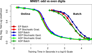
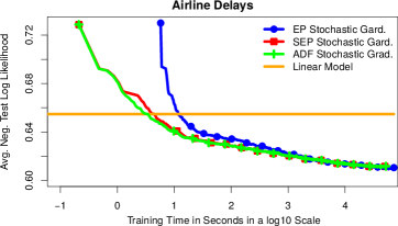
Figure 2: (top) Avg. negative test log likelihood for EP, SEP and ADF as a function of time. We show results when using a minibatch size $200$ for training (stochastic) and when using all data instances at once (batch). The performance of a linear logistic regression classifier is also shown for the airline dataset. Best seen in color.

Performance on big datasets: We carry out experiments when the model is trained using minibatches. We follow [10] and consider the MNIST dataset, which has 70,000 instances, and the airline delays dataset, which has 2,127,068 data instances (see [10] for more details). In both cases the test set has 10,000 instances. Training is done using minibatches of size 200, which is equal to the number of inducing points $m$. In the case of the MNIST dataset we also report results for batch training (in the airline dataset batch training is infeasible). Figure 2 shows the avg. negative log likelihood obtained on the test set as a function of training time. In the MNIST dataset training using minibatches is much more efficient. Furthermore, in both datasets SEP performs very similar to EP. However, in these experiments ADF provides equivalent results to both SEP and EP. Furthermore, in the airline dataset both SEP and ADF provide better results than EP at the early iterations, and improve a simple linear model after just a few seconds. The reason is that, unlike EP, SEP and ADF do not initialize the approximate factors to be uniform, which has a significant cost in this dataset.

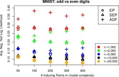
Figure 3: Performance of each method (ADF, SEP and EP) on the MNIST dataset for increasing training set sizes $n$ and model complexity (# inducing points $m$).

Dataset size and model complexity: The results obtained in the large datasets contradict the results obtained in the UCI datasets in the sense that ADF performs similar to EP. We believe the reason for this is that ADF may perform similar to EP only when the model is simple (small $m$) and/or when the number of training instances is very large (large $n$). To check that this is the case, we repeat the experiments with the MNIST dataset with an increasing number of training instances $n$ (from $1,000$ to $20,000$) and with an increasing number of inducing points $m$ (from $50$ to $400$). The results obtained are shown in Figure 3, which confirms that ADF only performs similar to EP in the scenario described. By contrast, SEP seems to always perform similar to EP. Finally, increasing the model complexity ($m$) seems beneficial.

5 Conclusions

Stochastic expectation propagation (SEP) [11] can reduce the memory cost of the method recently proposed in [10] to address large scale Gaussian process classification. Such a method uses expectation propagation (EP) for training, which stores $\mathcal{O}(nm)$ parameters in memory, where $m\ll n$ is some small constant and $n$ is the training set size. This cost may be too expensive in the case of very large datasets or complex models. SEP reduces the storage resources needed by a factor of $n$, leading to a memory cost that is $\mathcal{O}(m^{2})$. Furthermore, several experiments show that SEP provides similar performance results to those of EP. A simple baseline known as ADF may also provide similar results to SEP, but only when the number of instances is very large and/or the chosen model is very simple. Finally, we note that applying Bayesian learning methods at scale makes most sense with large models, and this is precisely the aim of the method described in this extended abstract.

Acknowledgments: YL thanks the Schlumberger Foundation for her Faculty for the Future PhD fellowship. JMHL acknowledges support from the Rafael del Pino Foundation. RET thanks EPSRC grant #s EP/G050821/1 and EP/L000776/1. TB thanks Google for funding his European Doctoral Fellowship. DHL and JMHL acknowledge support from Plan Nacional I+D+i, Grant TIN2013-42351-P, and from Comunidad Autónoma de Madrid, Grant S2013/ICE-2845 CASI-CAM-CM. DHL is grateful for using the computational resources of Centro de Computación Científica at Universidad Autónoma de Madrid.

References

- [1] C.E. Rasmussen and C.K.I. Williams. Gaussian Processes for Machine Learning. The MIT Press, 2006.
- [2] H. Nickisch and C.E. Rasmussen. Approximations for binary Gaussian process classification. Journal of Machine Learning Research, 9:2035–2078, 2008.
- [3] J. Quiñonero Candela and C.E. Rasmussen. A unifying view of sparse approximate Gaussian process regression. Journal of Machine Learning Research, pages 1935–1959, 2005.
- [4] E. Snelson and Z. Ghahramani. Sparse Gaussian processes using pseudo-inputs. In Advances in Neural Information Processing Systems 18, 2006.
- [5] A. Naish-Guzman and S. Holden. The generalized FITC approximation. In Advances in Neural Information Processing Systems 20. 2008.
- [6] J. Hensman, A. Matthews, and Z. Ghahramani. Scalable variational Gaussian process classification. In Proceedings of the Eighteenth International Conference on Artificial Intelligence and Statistics, 2015.
- [7] M. Titsias. Variational Learning of Inducing Variables in Sparse Gaussian Processes. In International Conference on Artificial Intelligence and Statistics (AISTATS), 2009.
- [8] M.D. Hoffman, D.M. Blei, C. Wang, and J. Paisley. Stochastic variational inference. Journal of Machine Learning Research, 14:1303–1347, 2013.
- [9] T. Minka. Expectation propagation for approximate Bayesian inference. In Annual Conference on Uncertainty in Artificial Intelligence, pages 362–36, 2001.
- [10] D. Hernández-Lobato and J. M. Hernández-Lobato. Scalable Gaussian process classification via expectation propagation. ArXiv e-prints, 2015. arXiv:1507.04513.
- [11] Y. Li, J. M. Hernández-Lobato, and R. Turner. Stochastic expectation propagation. In Advances in Neural Information Processing Systems 29, 2015.
- [12] P. S. Maybeck. Stochastic models, estimation and control. Academic Press, 1982.
- [13] Y. LeCun, L. Bottou, Y. Bengio, and P. Haffner. Gradient-based learning applied to document recognition. Proceedings of the IEEE, 86(11):2278–2324, 1998.