TemplateNet for Depth-Based Object Instance Recognition

Abstract

We present a novel deep architecture termed templateNet for depth based object instance recognition. Using an intermediate template layer we exploit prior knowledge of an object’s shape to sparsify the feature maps. This has three advantages: (i) the network is better regularised resulting in structured filters; (ii) the sparse feature maps results in intuitive features been learnt which can be visualized as the output of the template layer and (iii) the resulting network achieves state-of-the-art performance. The network benefits from this without any additional parametrization from the template layer. We derive the weight updates needed to efficiently train this network in an end-to-end manner. We benchmark the templateNet for depth based object instance recognition using two publicly available datasets. The datasets present multiple challenges of clutter, large pose variations and similar looking distractors. Through our experiments we show that with the addition of a template layer, a depth based CNN is able to outperform existing state-of-the-art methods in the field.

1 Introduction

Recent advances in computer vision has led to deep learning algorithms matching and outperforming humans in various recognition tasks like digit recognition [28], face recognition [29] and category recognition [15]. A common theme among them is the use of additional techniques to better regularise the training of a network with large number of parameters. For instance, using dropout, Srivastava et al. prevent co-adaptation and overfitting [28]. Similarly, using batch normalization, Ioffe & Szegedy [15] reduce the degrees of freedom in the weight space. This encourages us to explore more ways to regularise such large models by designing problem-specific regularizers.

A popular approach for regularisation is to introduce sparsity into the model [23]. However existing schemes of introducing sparsity in deep networks generally cannot be trained in a end-to-end manner and require a complex alternating schemes of optimization [24, 19]. Moreover, in most of these methods (including dropout) the sparse feature maps lack spatial structure. Based on the application domain it might be possible to leverage prior knowledge to introduce structure to the sparsity. Depth-based instance recognition is one such application where we have a complete 3D scan of an object during training and the goal is to recognize it under different viewpoints in challenging 2.5D test scenes. We take advantage of this prior information by employing an intermediate template layer to introduce structure to the sparse feature maps. We call this new architecture TemplateNet and derive weight update equations to train it in an end-to-end manner. We show that with the additional regularisation of the template layer, templateNet outperforms existing state-of-the-art methods in depth based instance recognition.

In addition to introducing sparsity, observing the output of a template layer allows us to visualize the learnt features of an object. This is a more natural way of visualizing learnt features as compared to existing methods which either use redundant layers [32] that are not useful for inference or need to backpropagate errors while maximizing class probability using additional constrains to obey natural image statistics [27].

In summary our main contributions in this paper are:

• For the task of instance recognition, using a template layer we impose structure on the sparse activations of feature maps. This regularises the network and improves its performance without additional parametrization.

• The output of template layer can be used to visualize the learnt features for an object.

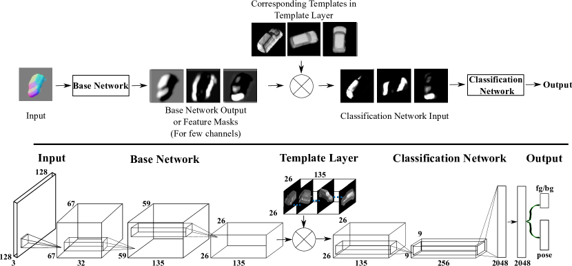
Figure 1: Top pane: A block diagram view of our proposed architecture. TemplateNet contains three modules (see section 3): (a) Base network: extracts the feature masks; (b) Template layer: introduces sparsity to the feature masks using prior knowledge; (c) Classification network: outputs the final predictions. TemplateNet allows us to visualize these intermediate feature masks giving an intuition of the learnt features. For more visualization results please see figure 3. Bottom pane: The final architecture that we use in our experiments. The numbers quoted correspond to the image/feature map dimensions and the number of channels used.

2 Literature Review

The advancement in sensor technology [20, 8] coupled with real time reconstruction systems [22] has resulted in depth data being readily available. Encouraged by this several methods on instance recognition using depth data have been proposed. One of the most popular is that of Hinterstoisser et al. [10] which uses surface normals from depth images together with edge orientations from RGB images as template features. Using a fast matching scheme the authors match thousands of such template features from different viewpoints of the object to robustly detect the presence of an object. However the lack of discriminative training leads to poor performance in presence of similar looking clutter.

Brachmann et al. [3], use a random forest to perform a per pixel object pose prediction. Using an energy minimization scheme they compute the final pose and location of an object in the scene. In contrast to their multi-stage approach we use end-to-end learning to detect both the location and pose of an object. In [31] rather than using discriminative training, Tejani et al. use co-training with hough forest. This avoids the need for background/negative training data. However during testing it requires multiple passes over the trained forest to predict the location and pose of the object. Moreover, in the absence of negative data it is unclear how this method can perform in the presence of similar looking clutter. In [2] using soft labelled random forest (slRF) [6], Bonde et al. perform discriminative learning on the manually designed features of [10] and show impressive performance under heavy as well as similar looking clutter using only the depth data. With CNN’s [18] driving recent advances in computer vision we explore its use in depth based instance recognition for performing feature learning. As our experiments show (section 4), we need to regularise the CNN to compete with existing methods.

Sparsity has been widely used for better regularisation in both shallow architectures [23] as well as in deep architectures [19]. A popular approach to enforce sparsity in deep architectures is to use an $L1$ norm penalty on the filter weights. Ranzato et al. showed that better structured filters are obtained by enforcing sparsity on the output of the filters (or feature maps) rather than the filter weights [24]. To achieve this they use a sparsifying logistic which converts the intermediate feature maps to a sparse vector. However this results in a non-trivial cost function requiring a complex alternating optimization scheme for computing weight updates. We propose an alternate manner of introducing sparsity by using the template layer. We exploit the nature of the instance recognition problems by using prior knowledge of the object shape to introduce structure to the sparse activations of feature maps. This results in weight updates that can be easily computed for the entire network using the chain rule, thus allowing us to train the network in an end-to-end manner (section 3.1.3). Our proposed network outperforms existing methods on challenging publicly available datasets.

3 TemplateNet

Figure 1 (top pane) presents the architecture of templateNet. The templateNet essentially contains three components: the base network, the template layer and the classification network. The base network and the classification network contain standard convolutional layers (or fully connected layers). On the other hand, a template layer is essentially an element wise multiplicative layer having one-to-one connection with the base networks output. To better motivate the function of each component in a templateNet we first draw connections to existing methods in literature for instance recognition.

Figure 2 shows the block diagram representations of different approaches. The top left pane shows the block diagram for LineMod [10] which consists of four blocks. In LineMod, given the input, it is first filtered using a manually designed orientation filter bank. These filtered responses are then matched with object template feature masks which are manually designed and tuned to highlight sparse discriminative features (such as edges or corners) for each template of an object. Finally, either using a learnt classifier or a scoring function, the input is classified as foreground or background. As these blocks are manually designed we have a good understanding of this system and how it learns to recognize different objects.

The top right pane shows the block diagram of the slRF-based instance recognition system of [2] where the discriminative features (or feature masks) are learnt across different templates. Visualizing the features used by the split nodes gives an understanding of the learnt feature masks. Bottom left pane shows the block diagram of a typical feed-forward CNN. Here an end-to-end system is used to learn the filter banks as well. Although methods have been proposed to visualize these deep networks [32, 27] they either require redundant layers or additional optimization steps.

In templateNet, shown in the bottom right pane of figure 2, we split the deep neural network into two separate networks with an additional template layer inserted between them (figure 1). The base network learns the orientation filters and the feature masks for templates. Ideally, we want these feature mask to be sparse and contain only the discriminative features. However, rather than enforcing sparsity on the feature masks we use the template layer as a sparsity inducing module. The weights of a template layer correspond to different template views of the object. As these templates have structured shapes they force the template layer output to also contain structure in their sparse activation (figure 1 and 3). This is in contrast to [24] which does not enforce any spatial structure to their sparse feature maps. Finally, the classification network uses these sparse maps as input to make the predictions.

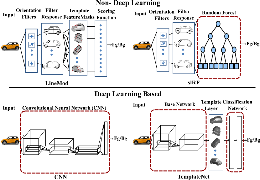
Figure 2: Block diagram view of different approaches to instance recognition. Top left is the block diagram for Template Matching (LineMod [10]) which uses manually designed filter banks and distinguishing feature (or feature masks) giving a better understanding of the system. Top right is the discriminative method using slRF [2]. The discriminative features are learnt and can be visualized by plotting high frequency split node questions. The base filters banks are however manually designed. Bottom left is the block diagram for a typical convolutional neural network which learns the filters as well as the discriminative features. Visualizing them however needs additional trained filters or optimization steps. Bottom right is our proposed TemplateNet which also performs end-to-end learning. Plotting the output of a template layer is a simple way to visualize the learnt features (figure 3).

Visualizing the template layer output is an intuitive way to understand the learnt features. Figure 3 shows these learnt responses for each template in the template layer of object class Mini in the dataset Desk3D [2]. The first column in each pane shows the learnt feature masks which is the output of base network. The second column shows the templates used in the fixed template layer. The final column is the rectified linear output of the element wise product between first two columns and is the input for the classification network. We also highlight some of the intuitive features learnt by this network such as edge orientation (shown in red) and surface orientation (shown in green). For clarity, in each row, the input used in the base network was the same as that in the corresponding template layer. Similar results were observed with different inputs. In the next section we explain the various aspects of training the templateNet.

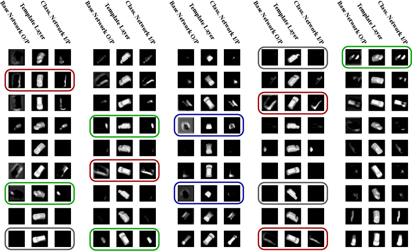
Figure 3: Interpreting templateNet: Learnt feature mask responses from our proposed templateNet for class Mini. We highlight some intermediate features learnt by the first network. In red we highlight edge orientation features, in green we highlight surface orientations. Lack of orientation, i.e high for everything but a specific orientation is shown in blue. Gray shows voids, i.e no features learnt. Here we show the responses only corresponding to one surface normal orientation. Similar observations were made with other channels.

3.1 Depth-based Instance recognition

Given the depth image of a scene, various maps such as height from ground plane, angle with gravity vector, curvature [9] can be computed to be used as input. However, here we follow existing methods on instance recognition which show state-of-the-art performance using surface normal features [10, 2]. These features can be efficiently computed using depth maps. We normalize each channel of the surface normal (x,y,z) in the range of $[0,1]$ and use it as our input. The template layers weights are also given by the surface normals of the corresponding template view. We use 45 different viewpoints (5 along yaw, 3 along pitch and 3 along roll) for each channel giving a total of $135$ ($45\times 3$) templates in the template layer.

3.1.1 OrthoPatch

As we use calibrated depth sensors we can leverage the physical dimensions encoded in a depth image to avoid searching over multiple window sizes. For this reason, using the camera calibration matrix, we compute the world co-ordinates from a depth image. We then perform orthogonal projections of the scene to get its orthoPatch. The resulting orthoPatch encodes the physical dimensions to a fixed scale thus removing the need to search over multiple scales.

3.1.2 Training

During training, we use a 3D model of the object and project it from different viewpoints. We simulate background clutter by randomly adding other objects along with floor before computing its orthoPatch. To improve robustness we also add random shifts. We crop this to $128\times 128$ dimension and simulate $27000$ such views to get the foreground (fg) training data. For background (bg) training data we use $128\times 128$ orthopatches from frames of video sequences containing random clutter to obtain the final training set $\mathbb{X}$.

Most methods in depth-based instance recognition rely on ICP [1] or its robust versions to get the final pose estimate of an object. Their primary focus is on having a good prediction for ICP initialization. We use a similar scheme and treat pose as a classification task rather than regression. To this end, we uniformly quantize object viewpoints into 16 pose classes with the goal of predicting the closest pose class. We thus have a $16+1$ (poses + background) pose classification task. As a test-object pose could be between two quantized pose classes rather than forcing the network to assign a specific quantized pose we use soft-labels [5]. This helps to better explain simulated poses that are not close to any single pose class. Soft labels for each simulated example are assigned based on the deviation of its canonical rotational matrix to the identity matrix [14]. For example, if $R_{i}^{j}$ represents the canonical rotation matrix which takes the $i^{th}$ simulated view to the $j^{th}$ quantized pose, then its distance is given by: $d_{i}^{j}=\|I-R_{i}^{j}\|_{F},$ where $I$ is a $3\times 3$ identity matrix and $\|.\|_{F}$ is the Frobenius norm. The soft labels are then given by: $l_{i}^{j}=\exp(-{d_{i}^{j}}^{2}),j\in\left\{1,...,16\right\}$. The final label vector $l_{i}$ is normalized to get the soft labels.

During testing, the sum of predicted labels across all quantized pose classes is used to estimate the foreground probability ($p_{fg}$). However, as we show later in our experiments, using this as the labels for training is not an optimal approach for detection. This is because a model learnt with only the pose classification cost does not explicitly maximize foreground probability.

In order to address both tasks of fg-bg and pose classification we take inspiration from the work of transforming auto-encoders [12]. We use a two-headed model with one head predicting the fg-bg probability which is invariant over the viewing domain. The other head predicts pose class probability which varies uniformly over the viewing domain and is similar to their instantiation parameters. This explicitly introduces the fg-bg objective into the cost function. The final cost function is given by the cross entropy as:

$$\begin{array}[]{l}\textbf{L}(\theta)=\frac{1}{N}\sum_{n=[1,\cdots,N]}-\textbf{L}^{n}\\ \textbf{L}^{n}=\sum_{i=[1,2]}\textbf{y}_{i}^{c}log(\textbf{p}_{i}^{c}(\theta))+\lambda\sum_{j=[1,17]}\textbf{y}_{j}^{p}log(\textbf{p}_{j}^{p}(\theta))\end{array}$$ (1)

Here the first term is the cross entropy for fg-bg classification with $y_{i}^{c}$ taking binary values (superscript $c$ indicating fg-bg) and the second term is for pose classification with $y_{j}^{p}$ given by the soft labels (superscript $p$ indicating pose). $\theta$ are the parameters of the network. We suppress the superscript $n$ from the second equation for clarity. $\lambda$ acts as the reweighing term to normalize the two cost functions. The resulting model with a mixed objective outperforms other single headed models that consider fg-bg and pose separately.

3.1.3 Learning

The individual components in templateNet can be formulated as:

• Base network can be simplified as a single convolutional layer with non-linearity: $\hat{\textbf{z}}=\phi(\widehat{W}^{T}\textbf{x}+\widehat{\textbf{b}})$

• Template layer can be formulated as a multiplicative layer with non-linearity: $\textbf{z}=\phi(\hat{\textbf{z}}\cdot T)$

• Classification network can be approximated as a softmax layer: $\textbf{p}=\sigma(W^{T}\textbf{z}+\textbf{b})$

where, x is the input, $\widehat{W}$,$W$ and $\widehat{\textbf{b}}$,b are the filter weights and biases, $T$ are the templates (or scaling factors), $\phi$ is the non-linearity (ReLU), $\sigma$ is the softmax function and p is the final predicted probability. Thus the parameters of the network are $\theta=\{\widehat{W},W,\widehat{\textbf{b}},\textbf{b},T\}$. We use the mixed cross entropy cost (equation (1)) as our cost function for training. We start from the classification network where the predicted probability is given as:

$$\textbf{p}_{i}=\frac{e^{-[W_{i}^{T}\textbf{z}+\textbf{b}_{i}]}}{\sum_{j}e^{-[W_{j}^{T}\textbf{z}+\textbf{b}_{j}]}}=\frac{e^{-[W_{i}^{T}\textbf{z}+\textbf{b}_{i}]}}{\textbf{Z}}$$ (2)

Subscripts $i$ and $j$ are used to index the $i^{th},\,j^{th}$ components of a vector (bold lower case variables) or the $i^{th},\,j^{th}$ columns of a matrix (upper case variables). Using the cross entropies per example term ($\textbf{L}^{n}$) from (1) (summation over $n$ is independent of $\theta$), the partial derivatives for classification network with respect to fg-bg cost are given by:

$$\frac{\partial\textbf{L}^{n}}{\partial W_{i}^{c}}=\textbf{y}_{i}^{c}\left[\textbf{z}-\frac{\textbf{z}e^{-[W_{i}^{c\;T}\textbf{z}+b_{i}^{c}]}}{\textbf{Z}^{c}}\right]$$

and

$$\frac{\partial\textbf{L}^{n}}{\partial b_{i}^{c}}=\textbf{y}_{i}^{c}\left[1-\frac{e^{-[W_{i}^{c\;T}\textbf{z}+b_{i}^{c}]}}{\textbf{Z}^{c}}\right]$$

The derivatives with respect to pose cost are the same with the additional reweighing term $\lambda$. Partial derivatives with respect to the input z is given by:

$$\frac{\partial\textbf{L}^{n}}{\partial\textbf{z}}=\sum_{i=[1,2]}\textbf{y}_{i}^{c}\left[W_{i}^{c}-\frac{\sum_{k=[1,2]}W_{k}^{c}e^{-[W_{k}^{c\;T}\textbf{z}+b_{k}^{c}]}}{\textbf{Z}^{c}}\right]+$$

$$\lambda\sum_{j=[1,17]}\textbf{y}_{j}^{p}\left[W_{j}^{p}-\frac{\sum_{l=[1,17]}W_{l}^{p}e^{-[W_{l}^{l\;T}\textbf{z}+b_{l}^{p}]}}{\textbf{Z}^{p}}\right]$$

Using chain rule we compute the partials derivatives with the template layer as:

$$~{}\frac{\partial\textbf{L}^{n}}{\partial T}=\frac{\partial\textbf{L}^{n}}{\partial\textbf{z}}\frac{\partial\textbf{z}}{\partial T}=\frac{\partial\textbf{L}^{n}}{\partial\textbf{z}}\;\phi^{\prime}(\hat{\textbf{z}}\cdot T)\hat{\textbf{z}}\;\;\;\;$$ (3)

and

$$\frac{\partial\textbf{L}^{n}}{\partial\hat{\textbf{z}}}=\frac{\partial\textbf{L}^{n}}{\partial\textbf{z}}\frac{\partial\textbf{z}}{\partial\hat{\textbf{z}}}=\frac{\partial\textbf{L}^{n}}{\partial\textbf{z}}\;\phi^{\prime}(\hat{\textbf{z}}\cdot T)T$$

where, $\phi^{\prime}$ is the derivative of ReLU which is equal to one for positive values and zero otherwise. Finally the partial derivatives with respect to masked response network parameters are given by:

$$\frac{\partial\mathbf{L}}{\partial\widehat{W}}=\frac{\partial\mathbf{L}}{\partial\hat{\textbf{z}}}\frac{\partial\hat{\textbf{z}}}{\partial\widehat{W}}=\frac{\partial\textbf{L}^{n}}{\partial\hat{\textbf{z}}}\;\phi^{\prime}[\widehat{W}^{T}\textbf{x}+\widehat{\textbf{b}}]\;\textbf{x}$$

$$\frac{\partial\mathbf{L}}{\partial\widehat{\textbf{b}}}=\frac{\partial\mathbf{L}}{\partial\hat{\textbf{z}}}\frac{\partial\hat{\textbf{z}}}{\partial\widehat{\textbf{b}}}=\frac{\partial\textbf{L}^{n}}{\partial\hat{\textbf{z}}}\;\phi^{\prime}[\widehat{W}^{T}\textbf{x}+\widehat{\textbf{b}}]$$

In the current work we do not update the $T$ and set $\frac{\partial\textbf{L}^{n}}{\partial T}=0$. However in future we could use (3) to update the template layer weights as well. To enforce sparsity an additional term such as penalizing $||T_{i}||_{1}$ might be needed. As the template layer weights are fixed it does not result in any additional training parameters. We train the templateNet in an end-to-end way similar to a typical CNN.

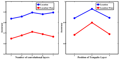
Figure 4: Location and location+pose accuracies for: left pane shows the performance with increasing convolutional layers for an object from Desk3D and right pane shows the performance for different positions of the template layer in templateNet.

3.2 Analysis

In this section we analyse the effect of different settings of templateNet and use them as a guide for further experiments in section 4.
Number of Convolutional layers: We test the effect of increasing the number of convolutional layers using the two headed network for a typical CNN. Figure 4 (left pane) compares the performance for class Kettle in Desk3D. We use the same training protocol of hardmining for all settings, i.e starting with a random subset of training data $\mathbb{X}_{s}\in\mathbb{X}$ followed by hard-mining after every 5-10 epochs for a total of 50 epochs. From the plot we observe the performance to start overfitting after five layers. Following these results we use five convolutional layers with two fully-connected layer as our base model for all other experiments.
Depth of Template layer: As a template layer is essentially a multiplicative layer it can be placed between any two convolutional layers. We experiment by placing the template layer at different depths in the five-layered CNN. Figure 4 (right pane) compares the resulting performance. Having more convolutional layers before the template layer leads to a larger non-linearity and hence more complex features to be learnt resulting in an improved performance. However as the template layer moves further from the input its regularisation effect on the initial filters reduces and the performance degrades. We found the templateNet performs best when the template layer is placed after the third convolutional layer in the five layered CNN. Figure 1 (bottom pane) shows the final architecture of templateNet.
First layer filters: The left pane of figure 5 shows the learnt filters in the first layer of our five-layered CNN. The noisy and unstructured first layer filters in the five-layered CNN can be accounted for by two factors: a) the model is over-parametrized; b) the model is not well regularised. However, from figure 4 (left pane) we observe that the test error decreases with an increase in number of layers (or parameters). This suggests that over-parametrization is not the primary cause and that the model is not well regularised. In comparison, the sparsity induced by the template layer regularises the templateNet and forces the filters to explain the data better making them structured and less noisy [21]. We observe this effect in figure 5 (right pane).

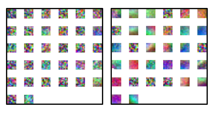
Figure 5: First layer filters of different networks. Left pane shows the filters learnt by a five-layered network using surface normals from depth images which look random and lack structure. Right pane compares the filters learnt by the templateNet. Due to stronger regularisation in templateNet most of the resulting filters have better structure.

4 Experiments and Results

Several datasets exist in the literature for testing instance recognition algorithms [17, 4, 30]. Of these we choose the Desk3D [2] and the ACCV3D [11] datasets. Unlike other datasets the Desk3D dataset contains separate scenarios to test the performance of the recognition algorithms under different challenges of similar looking distractors, pose change, clutter and occlusion. The controlled test cases allows us to better analyse each algorithm to estimate their performance under real world conditions. However ,this dataset is of a limited size and for this reason we also experiment with the ACCV3D dataset which is the largest publicly available labelled dataset covering large range of pose variations with clutter and multiple object shapes.
Benchmarks: Two different benchmarks are used to quantify and compare different settings. We use the state-of-the-art slRF method [2] together with the depth-based LineMod [10] as our base benchmarks. Since LineMod learns templates for RGB and depth separately, removing one modality does not affect the other. For reference we also report results from depth+HoG based DPM [7].

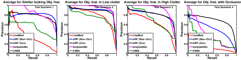
Figure 6: Precision-Recall curves for pose+location for different test scenarios in Desk3D. TemplateNet learns features directly from the input data and is more confident in its predictions. The template layer introduces sparsity and regularises the network. The resulting architecture improves performance over traditional CNN and outperforms previous state-of-the-art methods of LineMod and in three out of four challenges ((a) similar objects, (b) large pose variations and (c) clutter). As templateNet does not encode the occlusion information it fails on occluded scenes (d).

Testing Modality: We follow the same testing modality as [2]. We consider an object to be correctly localized if the predicted centre is within:$\frac{max(w,d,h)}{3}$ radius of the ground truth. For pose classification we consider pose to be correctly classified if the predicted pose class $p_{ps}^{*}$ given by: $p_{ps}^{*}=\operatorname*{arg\,max}_{i}p_{ps}^{i}$ i.e, largest pose probability is either the closest or second closest quantized pose to the ground truth.

	DPM [7]	LineMod	slRF [2]	CNN3	CNN3	CNN5	templateNet	templateNet
Object	(D-HoG)	[10]	(Normals)	(Pose)	(Mix)	(Mix)	(Mix-45)	(Mix-128)
Face	44.74	66.60	69.90	67.22	62.89	67.84	70.72	72.63
Kettle	53.34	60.49	83.75	72.31	70.55	72.49	84.13	89.07
Ferrari	32.41	47.90	50.42	59.66	69.75	68.07	81.51	80.11
Mini	30.64	55.09	63.74	36.54	57.74	60.53	77.96	76.78
Phone	64.32	79.03	91.85	80.94	69.67	70.54	83.36	90.81
Statue	70.29	84.76	81.97	39.22	50.37	55.95	83.09	84.92
Average	49.29	65.64	73.64	59.31	63.49	65.90	80.13	82.39

Table 1: Location+Pose accuracies on non-occluded scenes of Desk3D. We compare the templateNet with different settings of the convolutional neural network (CNN) together with previous state-of-the-art methods. Using the mixed cost function (mix) performs better than the pose+background cost (pose). Increasing the number of convolutional layers further improves the accuracy. However as CNN is not well regularised it still lags behind the state-of-the-art methods of LineMod [10] and slRF [2] (normal based). TemplateNet uses the template layer to enforce sparsity resulting in top performance in 4 out of 6 instances and the best overall performance. Increasing the number of templates from 45 to 128 results in further improvement but at a cost of large processing time. The results with larger templates (Mix-128) are only quoted for reference. We do not use them for other experiments. To avoid clutter we report only the location+pose accuracies and not the location only accuracies. Similar results were observed with location accuracies as well.

4.1 Experiments on Desk3D

The Desk3D dataset contains a total of six objects with 400-500 test scenes each. The test scenes are obtained by fusing few consecutive frames ($\approx 5$) using [25]. Figure 6 shows PR curves for the four different scenarios in Desk3D. Figure 6 (a) compares the performance on scenario 1 which consists of similar looking distractors. As the templateNet performs feature learning it outperforms other methods which use manually designed features. In figure 6 (b) we compare the performance for the low clutter and high pose variations stetting (scenario 2). TemplateNet is more confident for large pose variations and we observe a high precision for over 50% recall rates. A similar improvement is observed even with large cluttered background of scenario 3 (figure 6 (c)). Due to a better separation between foreground-background the templateNet is more confident even with large cluttered background giving high precision at large recalls.

In all three scenarios (6 a,b and c) the five layered CNN performs the worst compared to other benchmarks indicating a need for better regularisation. The templateNet achieves this using the sparsity inducing template layer resulting in the best performance.

Table 1 lists the accuracies of different settings for non-occluded scenes. For fairness we do not add dropouts in any of the architectures. The use of a mixed cost helps improve performance over a pose classification cost. This is because a model trained with the pose only cost does not explicitly maximize the foreground probability. With an increase in the number of layers the performance improves and saturates around five convolutional layers (figure 4). Using better regularisation our templateNet outperforms all others in four out of six objects and achieves the best overall accuracy. We also experiment with the width of the template layer i.e, number of templates used. As the number of templates increases we increase the representation power/dimensions of template layer while still regularising the network due to sparse activations. This leads to an improved performance of the network seen in the last column of table 1 albeit at a higher computational cost. For this reason we only report these results for reference.

The only scenario where templateNet suffers is under occlusion (figure 6 (d)). Using occlusion information the slRF outperforms templateNet when objects are partially occluded. In future using occlusion information could help the templateNet handle partially occluded scenes.

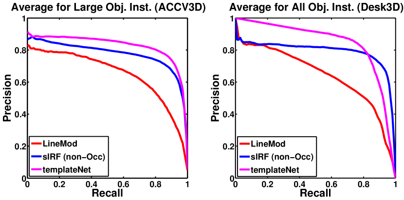
Figure 7: Precision-Recall curves for pose+location: left pane shows the performance on large objects (bounding box $>1000cm^{3}$) of ACCV3D dataset. Right pane shows the average performance for non-occluded scenes of Desk3D (Test scenarios 1,2 and 3).

4.2 Experiments on ACCV3D

The ACCV3D dataset contains $15$ different objects each with over $1100$ test scenes covering a range of poses. However we only experiment with $9$ large objects (bounding box $>1000$cc). This is because due to low sensor resolution the smaller $6$ objects do not have enough discriminative features and perform poorly. This observations is also consistent with the results of [2]. As our simulated training examples do not contain any noise modelling our system is not robust to raw depth images which contain boundary and quantization noise together with missing depth values. For this reason we use the depth in-painting technique proposed in [26] to smooth the raw depth images and use them as our input.

Object	LineMod [10]		slRF [2]		templateNet
Instance	L	L + P	L	L + P	L	L + P
B.Vise	83.79	75.23	87.98	86.50	96.79	92.18
Camera	77.19	68.94	58.20	53.37	83.76	80.27
Can	83.70	69.57	94.73	86.42	95.31	87.88
Driller	94.70	81.82	91.16	87.63	91.16	81.14
Iron	83.51	75.43	84.98	70.75	89.58	82.64
Lamp	92.91	80.93	99.59	98.04	95.44	81.99
Phone	77.72	70.47	88.09	87.69	94.05	91.39
Bowl	98.11	19.22	98.54	30.66	91.08	32.15
Box	63.37	27.69	95.21	63.53	95.29	72.47
Average	84.00	63.26	88.62	73.64	92.50	78.01

Table 2: Location (L) and Location+Pose (L+P) accuracies on the ACCV3D dataset. We report accuracies only for large objects (bounding box $>1000$cc). Due to the poor resolution of depth sensors small objects do not perform well. We train a mixed cost templateNet with 45 templates. Our end-to-end learned network outperforms existing state-of-the-art methods in 6 out of 9 categories and gets the best overall performance.

Figure 7 (left pane) shows the average precision-recall curves for different methods and table 2 reports the performance on the large objects in ACCV3D dataset. Our end-to-end trained templateNet achieves the best performance on 6 out of the 9 objects and the best overall performance.

5 Discussions

In this section we discuss some of the limitations of the current architecture and suggest possible directions to address these drawbacks.

In the current work, templateNet does not reuse the bottom level features requiring one netwrok per object. This could be addressed by having multiple template layers working in parallel with an additional group sparsity penalty [13] on them. This would limit the number of template layers being active while reusing the existing layers making it more efficient and scalable.

The other drawback as shown in our experiments (section 4.1) is its poor performance in occluded scenes. With the use of spatial transformers [16] we could detect salient parts to perform part based recognition to address this limitation. Nevertheless, templateNet outperforms existing works on all other challenges of instance recognition using only depth data.

6 Conclusions

We presented a new deep architecture called templateNet for depth-based object instance recognition. The new architecture used prior knowledge of object shapes to introduce sparsity on the feature maps. This was achieved without any additional parametrization of training by using an intermediate template layer. The sparse feature maps implicitly regularised the network resulting in structured filter weights. By visualizing the output of a template layer we get an intuition of the learnt discriminative features for an object. We derived the weight updates needed to train the templateNet in an end-to-end manner. We evaluated its performance on challenging scenarios of Desk3D as well as on the largest publicly available ACCV3D dataset. We showed that the template layer helped improve performance over a traditional convolutional neural network and outperforms existing state-of-the-art methods.

7 Acknowledgements

This research was supported by the Boeing Company. We gratefully acknowledge Paul Davies for his inputs in making this work useful to the industry.

References

- [1] P. Besl and N. McKay. A method for registration of 3-D shapes. Transactions on Pattern Analysis and Machine Intelligence, 14(2):239–256, 1992.
- [2] U. Bonde, V. Badrinarayanan, and R. Cipolla. Robust Instance Recognition in Presence of Occlusion and Clutter. In European Conference on Computer Vision, ECCV 2014, 2014.
- [3] E. Brachmann, A. Krull, F. Michel, S. Gumhold, J. Shotton, and C. Rother. Learning 6d object pose estimation using 3d object coordinates. In European Conference on Computer Vision, ECCV 2014. 2014.
- [4] B. Browatzki, J. Fischer, B. Graf, H. Bülthoff, and C. Wallraven. Going into depth: Evaluating 2D and 3D cues for object classification on a new, large-scale object dataset. In International Conference on Computer Vision Workshops on Consumer Depth Cameras, ICCV Workshops 2011, 2011.
- [5] I. Budvytis, V. Badrinarayanan, and R. Cipolla. Label propagation in complex video sequences using semi-supervised learning. In British Machine Vision Conference, BMVC 2010, 2010.
- [6] A. Criminisi and J. Shotton. Decision forests for computer vision and medical image analysis. Springer Science & Business Media, 2013.
- [7] P. Felzenszwalb, D. McAllester, and D. Ramanan. A discriminatively trained, multiscale, deformable part model. In Computer Vision and Pattern Recognition, CVPR 2008, 2008.
- [8] E. Golrdon and G. A. Bittan. 3D geometric modeling and motion capture using both single and dual imaging, 2012. US Patent 8,090,194.
- [9] S. Gupta, R. Girshick, P. Arbeláez, and J. Malik. Learning rich features from RGB-D images for object detection and segmentation. In European Conference on Computer Vision, ECCV 2014. 2014.
- [10] S. Hinterstoisser, S. Holzer, C. Cagniart, S. Ilic, K. Konolige, N. Navab, and V. Lepetit. Multimodal templates for real-time detection of texture-less objects in heavily cluttered scenes. In International Conference on Computer Vision, ICCV 2011, 2011.
- [11] S. Hinterstoisser, V. Lepetit, S. Ilic, S. Holzer, G. Bradski, K. Konolige, and N. Navab. Model based training, detection and pose estimation of texture-less 3D objects in heavily cluttered scenes. In Asian Conference on Computer Vision, ACCV 2013, 2013.
- [12] G. Hinton, A. Krizhevsky, and S. Wang. Transforming auto-encoders. In Artificial Neural Networks and Machine Learning–ICANN 2011. 2011.
- [13] J. Huang and T. Zhang. The benefit of group sparsity. The Annals of Statistics, 38(4):1978–2004, 2010.
- [14] D. Huynh. Metrics for 3D rotations: Comparison and analysis. Journal of Mathematical Imaging and Vision, 35(2):155–164, 2009.
- [15] S. Ioffe and C. Szegedy. Batch normalization: Accelerating deep network training by reducing internal covariate shift. arXiv preprint arXiv:1502.03167, 2015.
- [16] M. Jaderberg, K. Simonyan, A. Zisserman, and K. Kavukcuoglu. Spatial Transformer Networks. arXiv preprint arXiv:1506.02025, 2015.
- [17] K. Lai, L. Bo, X. Ren, and D. Fox. A large-scale hierarchical multi-view rgb-d object dataset. In International Conference on Robotics and Automation, ICRA 2011, 2011.
- [18] Y. LeCun, L. Bottou, Y. Bengio, and P. Haffner. Gradient-based learning applied to document recognition. Proceedings of the IEEE, 86(11):2278–2324, 1998.
- [19] H. Lee, C. Ekanadham, and A. Y. Ng. Sparse deep belief net model for visual area V2. In Advances in neural information processing systems, NIPS 2008, 2008.
- [20] K. Litomisky. Consumer rgb-d cameras and their applications. Rapport technique, University of California, page 20, 2012.
- [21] R. Memisevic. Learning to relate images. Transactions on Pattern Analysis and Machine Intelligence, 35(8):1829–1846, 2013.
- [22] R. Newcombe, S. Izadi, O. Hilliges, D. Molyneaux, D. Kim, A. Davison, P. Kohli, J. Shotton, S. Hodges, and A. Fitzgibbon. KinectFusion: Real-time dense surface mapping and tracking. In International symposium on Mixed and augmented reality, ISMAR 2011, 2011.
- [23] B. Olshausen and D. Field. Sparse coding with an overcomplete basis set: A strategy employed by V1? Vision research, 37(23):3311–3325, 1997.
- [24] C. Poultney, S. Chopra, and Y. Cun. Efficient learning of sparse representations with an energy-based model. In Advances in neural information processing systems, NIPS 2006, 2006.
- [25] R. Rusu and S. Cousins. 3D is here: Point Cloud Library (PCL). In International Conference on Robotics and Automation, ICRA 2011, 2011.
- [26] N. Silberman, D. Hoiem, P. Kohli, and R. Fergus. Indoor segmentation and support inference from RGBD images. In European Conference on Computer Vision, ECCV 2012. 2012.
- [27] K. Simonyan, A. Vedaldi, and A. Zisserman. Deep inside convolutional networks: Visualising image classification models and saliency maps. arXiv preprint arXiv:1312.6034, 2013.
- [28] N. Srivastava, G. Hinton, A. Krizhevsky, I. Sutskever, and R. Salakhutdinov. Dropout: A simple way to prevent neural networks from overfitting. The Journal of Machine Learning Research, 15(1):1929–1958, 2014.
- [29] Y. Taigman, M. Yang, M. Ranzato, and L. Wolf. Deepface: Closing the gap to human-level performance in face verification. In Computer Vision and Pattern Recognition, CVPR 2014, 2014.
- [30] J. Tang, S. Miller, A. Singh, and P. Abbeel. A textured object recognition pipeline for color and depth image data. In International Conference on Robotics and Automation, ICRA 2012, 2012.
- [31] A. Tejani, D. Tang, R. Kouskouridas, and T.-K. Kim. Latent-class hough forests for 3D object detection and pose estimation. In European Conference on Computer Vision, ECCV 2014. 2014.
- [32] M. Zeiler, D. Krishnan, G. Taylor, and R. Fergus. Deconvolutional networks. In Computer Vision and Pattern Recognition, CVPR 2010, 2010.