Investigating the origin and spectroscopic variability of the near-infrared H I lines in the Herbig star VV Ser

Abstract

The origin of the near-infrared (NIR) H i emission lines in young stellar objects are not yet understood. To probe it, we present multi-epoch LBT-LUCIFER spectroscopic observations of the Pa$\delta$, Pa$\beta$, and Br$\gamma$ lines observed in the Herbig star VV Ser, along with VLTI-AMBER Br$\gamma$ spectro-interferometric observations at medium resolution. Our spectroscopic observations show line profile variability in all the H i lines. The strongest variability is observed in the redshifted part of the line profiles. The Br$\gamma$ spectro-interferometric observations indicate that the Br$\gamma$ line emitting region is smaller than the continuum emitting region. To interpret our results, we employed radiative transfer models with three different flow configurations: magnetospheric accretion, a magneto-centrifugally driven disc wind, and a schematic bipolar outflow. Our models suggest that the H i line emission in VV Ser is dominated by the contribution of an extended wind, perhaps a bipolar outflow. Although the exact physical process for producing such outflow is not known, this model is capable of reproducing the averaged single-peaked line profiles of the H i lines. Additionally, the observed visibilities, differential and closure phases are best reproduced when a wind is considered. Nevertheless, the complex line profiles and variability could be explained by changes in the relative contribution of the magnetosphere and/or winds to the line emission. This might indicate that the NIR H i lines are formed in a complex inner disc region where inflow and outflow components might coexist. Furthermore, the contribution of each of these mechanisms to the line appears time variable, suggesting a non-steady accretion/ejection flow.

1 Introduction

UX Orionis stars (UXORS) are pre-main sequence stars showing strong photometric variability at optical wavelengths. They receive their name after the prototype star UX Ori, a Herbig AeBe star. Most UXORS are, indeed, Herbig AeBe stars, although there are also some UXORS amongst Classical T Tauri stars (CTTSs) of early K spectral type such as RY Tau and RY  Lup. UXORS are characterised by sudden decreases in their optical brightness of up to 2-3 mag. During the faint state, UXORS become redder with a simultaneous increase of their polarisation. However, during deep minima these stars become bluer. These observational properties, that is the magnitude fading, the increase of polarisation and the bluing effect, suggest that UXORS faiding is due to extinction events caused by filaments or clouds of dust orbiting the central source and crossing the line of sight in a nearly edge-on disc (Grinin et al., 1991, 1998). A variation of this hypothesis was proposed by Dullemond et al. (2003) suggesting that UXORS events could only happen in self-shadowed disk geometries viewed at high inclination angles. In this model the inner disc is at the origin of the obscuring clouds, and it must have a puffed-up geometry. In addition to the obscuration hypothesis, disc instabilities, inhomogeneities or warps can also contribute to the dimming magnitude observed in UXORS stars. For instance, (Bouvier et al., 2013, and references therein) proposed a combination of these two scenarios to explain the complex photometric behaviour of AA Tau (Bouvier et al., 2013, and references therein). This source shows a low amplitude quasi-periodic variability that was explained by the presence of an asymmetric dusty warp at the disc inner edge caused by material lifted up from the disc plane by an inclined stellar magnetosphere. In addition to the low amplitude variability, AA Tau also shows deep minima consistent with a sudden increase of the dust extinction as predicted by the obscuration hypothesis.

Table 1: Total exposure times of the LBT observations.

UT Date	z	J	K
	(s)
2012-04-23	512	240	1280
2012-05-28	720	480	128
2012-06-23	720	240	64

Despite many photometric studies, very little spectroscopic monitoring of UXORS has been conducted. The few studied cases show dramatic changes in the spectroscopic line profiles, not always linked with photometric variability (Eaton & Herbst, 1995; de Winter et al., 1999; Natta et al., 2000; Rodgers et al., 2002). In addition, most of these studies investigate variability in the optical, usually focusing on the H$\alpha$ line.

In this paper we present a NIR spectroscopic monitoring of the UXOR Herbig AeBe star VV Ser. This source is located in the main Serpens molecular cloud at $\sim$415 pc (Dzib et al., 2010). There is some discrepancy in the literature about the photospheric temperature of VV Ser, but most studies identify VV Ser as an Herbig star of spectral type B. Montesinos et al. (2009) performed a complete study of the stellar properties of VV Ser, concluding that the most plausible temperature and age of this source is 13 800 K and 1.2 Myr, respectively. The light curve of VV Ser consists of small amplitude brightness variations around the bright state followed by rare non-periodical deep minima lasting of order of ten days (Rostopchina et al., 2001). The disc of VV Ser appears to be self-shadowed, of low mass, and viewed at a high inclination angle (i$\sim$70°; Pontoppidan et al., 2007). This would favour the obscuration hypothesis proposed by Dullemond et al. (2003) to explain the deep minima observed in VV Ser. In addition to the photometric variability typical of UXORS, VV Ser also shows spectroscopic line variability. In particular, optical spectroscopic studies show strong variability of the H$\alpha$ line profile (e.g., Mendigutía et al., 2011). To further constrain the structure of the inner gasseous disc of this source, additional medium-resolution interferometric observations are presented (Section 2.2). Previous spectro-interferometric observations of this source show a compact Br$\gamma$ emitting region, tracing gas located within the dust sublimation radius (Eisner et al., 2014, and references therein).

Table 2: Observation log of the VLTI/AMBER medium-resolution (R$\sim$1500) observations of VV Ser conducted with the UT1-UT2-UT4 configuration.

UT Date	UT Time	DIT	NDIT	Proj. baselines	PA	Calibrator	UD diameter
	[h:m]	[ms]	#	[m]	[$\circ$]		[mas]
2014-05-13	05:47–06:00	500	1200	47.66 / 76.34 / 104.98	-165.47 / -99.14 / -123.72	HD 163 272	$0.265\pm 0.020$
2012-05-13	06:27–06:40	500	1200	49.20 / 83.25 / 115.28	-156.67 / -98.40 / -120.38	HD 170 920	$0.285\pm 0.019$

This paper is structured as follows: The NIR spectroscopic and inteferometric observations along with the data reduction are presented in Sections 2.1 and 2.2. The results obtained from our observations are shown in Sections 3 (spectroscopy) and 4 (interferometry). The theoretical models employed to interpret our results can be found in Section 5, followed by a discussion (Section 6) and the conclusions (Section 7).

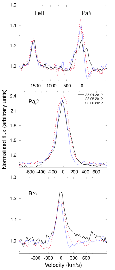
Figure 1: LBT MR spectroscopic observations of VV Ser. The H i line profiles are normalised to the continuum. The reported velocity is with respect to the local cloud velocity which is at an LSR velocity of +8 km s^-1 (Burleigh et al., 2013).

2 Observations and data reduction

2.1 Spectroscopic observations at medium resolution

VV Ser was observed during three different nights in 2012 (23 April, 28 May and 23 June) using the infrared spectrograph and camera LUCIFER, installed on the Large Binocular Telescope (LBT) at Mount Graham Observatory. For each night, medium-resolution (MR) spectra in the z-, J-, and K-band were acquired consecutively, using the N1.8 camera (grating 210_zJHK) and a slit width of 0$\aas@@fstack{\prime\prime}$5. This provides a spectral resolution of R$\sim$6700. The observations were performed using a spatial scale of 0.25″/pixel. Total exposure times for each date and band are listed in Table 1.

Data reduction was performed using standard IRAF tasks. Atmospheric OH lines were used for wavelength calibration. The atmospheric spectral response was corrected by dividing the object spectra by the spectrum of a telluric spectroscopic standard. With this aim, the intrinsic absorption features of the standard were removed before dividing the spectra by a normalised blackbody at the appropriate temperature. Finally, due to unstable seeing conditions as well as the presence of cirrus, no photometric calibration of the spectra was performed.

2.2 Near-IR interferometric observations

We observed VV Ser with the AMBER instrument of the Very Large Telescope Interferometer (VLTI) using the 8-m unit telescopes (UT’s) with the configuration UT1-UT2-UT4 during one night in May 2014. The AMBER instrument is a three beam combiner that records spectrally dispersed three-beam interferograms (Petrov et al., 2007). Due to the faint H-band magnitude of VV Ser (H$\sim$7.4) and poor atmospheric conditions (seeing$\sim$1″), the observations were conducted without the fringe tracker FINITO. We recorded K-band interferograms, within the Br$\gamma$ line and the nearby continuum, in the medium spectral resolution mode (R$\sim$1500) with a detector integration time (DIT) of 500 ms. To calibrate the atmospheric transfer function, we observed the calibrator stars HD 163272 and HD 170920. For data reduction, we employed the software library amdlib v3.0.5 (Tatulli et al., 2007; Chelli et al., 2009). We selected 20 per cent of the frames with the highest fringe SNR as described in Tatulli et al. (2007). The observation log is shown in Table 2.

3 Spectroscopic results

The most prominent features in our VV Ser spectra are hydrogen recombination emission lines, namely the Pa$\delta$ and Pa$\beta$ lines in the z- and J-band, and the Br$\gamma$ line in the K-band. In addition, strong emission from the fluorescent Fe ii 10000.3Å line is also observed in the z-band (Bautista et al., 2004; Johansson & Letokhov, 2004; Caratti o Garatti et al., 2013). Figure 1 shows the spectra of these lines, normalised to the continuum and calibrated in velocity for each of the three observation nights. All radial velocities are with respect to the cloud which is at a velocity of +8 km s^-1 with respect to the local standard of rest (LSR; Burleigh et al., 2013). The measured radial velocities and equivalent widths (EWs) of each line at each epoch are listed in Table 3. The errors in the radial velocity values were estimated by comparing the theoretical wavelength of the OH lines located close to the line of interest in the sky frames and the measured value after wavelength calibration.

The Fe ii line is roughly centred at zero velocity and does not show any significant line profile variability. On the other hand, all the hydrogen recombination lines are, on average, blueshifted with EWs ranging from $\sim-$3 Å, for the Br$\gamma$ line, to $\sim-$17 Å, for the Pa$\beta$. In addition, a night-by-night variation in the line EWs and line profiles is observed.

In particular, the Pa$\delta$ line shows a very complex line profile with a clear line profile variability. In the first epoch (black continuous line in Fig. 1), the Pa$\delta$ line shows three different velocity components, namely a blueshifted high velocity component (HVC) at $\sim$–173 km s^-1, a blueshifted low velocity component (LVC) at $\sim$–30 km s^-1, and a redshifted velocity component at $\sim$+120 km s^-1. In the second and third epoch (dotted blue and dashed red lines), the redshifted emission disappears as well as the blue-shifted double peak, leaving in its place an inverse P-Cygni profile. Similar redshifted emission components are also observed during the first epoch in the Pa$\beta$ and Br$\gamma$ lines as a redshifted bump in the line profiles. As for the Pa$\delta$ line profile, these redshifted bumps disappear during the second and third epochs. In contrast with the Pa$\delta$ line, the redshifted absorption component of the inverse P-Cygni profile is only marginally observed in the Br$\gamma$ line during the last epoch.

Table 3: Radial velocities.

	2012-04-23		2012-05-28		2012-06-23
Line id.	Vr	EW	Vr	EW	Vr	EW
	km s-1	Å	km s-1	Å	km s-1	Å
FeII	4.7$\pm$3.2	-1.9$\pm$0.6	-6.0$\pm$6.5	-1.8$\pm$0.3	-12.8$\pm$8.8	-1.9$\pm$0.5
Pa$\delta$	-29.5$\pm$3.2	-2.4$\pm$0.2	-73.0$\pm$6.5	-3.2$\pm$0.7	-42.8$\pm$8.8	-3.7$\pm$0.9
	119.6$\pm$3.2	-1.9$\pm$0.3
Pa$\beta$	-0.9$\pm$5.1	-15.8$\pm$1.0	-25.6$\pm$5.3	-13.0$\pm$0.7	-13.8$\pm$6.6	-16.7$\pm$1.4
Br$\gamma$	6.3$\pm$1.6	-4.1$\pm$0.5	-33.5$\pm$2.3	-3.0$\pm$0.5	-28.4$\pm$1.0	-4.2$\pm$1.2

On the other hand, the radial peak velocities increase from the first to the second epoch in all the H i lines, and they decrease from the second to the third epoch (see Table 3). The lowest radial velocities are observed during the first epoch. This is due to the redshifted bumps observed during this epoch that shift the centred of the line profile towards the line rest velocity. Almost the opposite behaviour is observed during the second epoch.

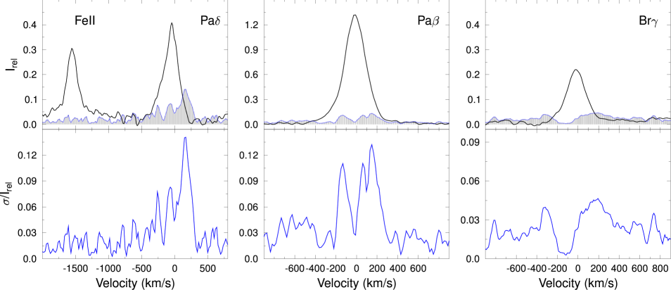
Figure 2: Top: From left to right, averaged line profile (I_rel) of the Fe ii 10000.3Å and Pa$\delta$ lines, the Pa$\beta$ line, and Br$\gamma$ line. The line profiles are normalised to the continuum, and shifted by -1. The normalised variance profiles as in bottom are overplotted (blue lines filled in grey) for comparison. Bottom: Same as in Top, but for the normalised variance line profiles ($\sigma$/I_rel) of the Fe ii and Pa$\delta$ lines, the Pa$\beta$ line, and the Br$\gamma$ line, respectively.

Similarly, EW variations are observed in the hydrogen recombination lines (see, Table 3). These changes give us relative information on the continuum to line flux variations, indicating possible changes in the line or continuum fluxes through the analysed period. Unfortunately, the lack of simultaneous NIR photometry prevents us from distinguishing between both possibilities. The measured EWs and errors are reported in Table 3. The EW error was estimated from:

$$\sigma(EW_{\lambda})=\sqrt{1+\frac{F_{c}}{F}}\frac{(\Delta\lambda-EW_{\lambda})}{S/N}$$ (1)

assuming Poisson-statistics for the computation of the flux error and standard error propagation (Vollmann & Eversberg, 2006). In this expression, $F_{c}$ and $F$ are the continuum and line flux, S/N is the signal-to-noise-ratio around the line position, and $\Delta\lambda$ is the wavelength interval over which the line EW was estimated. Both the Pa$\beta$ and Br$\gamma$ lines show night-to-night changes in their EWs. In particular, the EW decreases from the first to the second epoch in both lines, increasing again during the third epoch. Due to the complex Pa$\delta$ line profile, it is difficult to extract any quantitative conclusion on the EW behaviour of this line. However, as mentioned above this line shows a clear line profile variability.

To better quantify the line variability, the averaged and normalised variance profiles of the Pa$\delta$, Pa$\beta$, and Br$\gamma$ lines for the three epochs were computed (see, Fig. 2). Following Johns & Basri (1995), the normalised variance profiles ($\sigma_{k}$/I_rel,k) were derived by dividing the profile variance by the average line profile. The line profile variance was computed from:

$$\sigma_{k}=\Big{[}\frac{1}{(N-1)}\sum_{i=1}^{N}(I_{i,k}-I_{\mathrm{rel},k})^{2}\Big{]}^{1/2},$$ (2)

where $I_{i,k}$ denotes the intensity profile of the line $k$ at each single epoch, I_rel,k is the average profile of the line $k$, and $N$ is the number of epochs. The comparison of the averaged line profiles with the normalised variance profiles illustrates where the major changes in the line profiles take place (Johns & Basri, 1995; Kurosawa et al., 2005; Mendigutía et al., 2011). The most relevant changes across the line profiles affect the redshifted component of the line profiles, although smaller changes are also observed at blueshifted velocities. Notably, both Pa$\delta$ and Pa$\beta$ lines show similar normalised variance profiles, indicating that their variability originates from similar physical processes. However, the line to continuum ratio of the Pa$\delta$ line is smaller than that for Pa$\beta$, and therefore, the line profile variation is more evident in the former line. The sizes of the normalised variances are slightly smaller for the Br$\gamma$ line compared to those of the Pa$\beta$ and Pa$\delta$ lines. As the Br$\gamma$ line is optically thinner than the Pa$\beta$ and Pa$\delta$ lines, the line emitting volume for these latter would be larger than that of the Br$\gamma$. This might be the reason for the slightly larger variability observed in the Paschen lines.

3.1 Accretion properties

The accretion luminosity of VV Ser was estimated from the luminosity of the Br$\gamma$ line using the empirical relationship derived from Donehew & Brittain (2011). The Br$\gamma$ luminosity was derived from the EW of the line, once the intrinsic photospheric absorption contribution to the line was corrected (see Garcia Lopez et al., 2006; Donehew & Brittain, 2011, for more details). This leads to Br$\gamma$ photospheric-corrected equivalent widths (EW_circ) of 4.7, 3.6 and 4.8 Å for the first, second and third epoch, respectively. The stellar parameters used in the computation can be found in Table 5. In addition, a visual extinction of A_V=3.4 mag was assumed (Montesinos et al., 2009). The accretion luminosity ($L_{\mathrm{acc}}$) was estimated assuming a constant 2MASS K-band magnitude of the source of m_K=6.32. The average $L_{\mathrm{acc}}$ value over the three epochs is $\sim$15.8${}^{+9.3}_{-7.9}$ L_⊙. This leads to a mass accretion rate of $\dot{M}_{\mathrm{acc}}$$\sim$ 3.1${}^{+1.6}_{-1.5}\times$10^-7 M_⊙ yr^-1, assuming that $\dot{M}_{\mathrm{acc}}$= $L_{\mathrm{acc}}$ R_∗/ G M_∗. In this expression, R_∗ and M_∗ are the stellar radius and mass (see Table 5), and G is the universal gravitational constant.

Table 4: Geometric models

	Continuum			Line
	R	PA	$i$	$R$	PA	$i$
	(mas)	(deg)		(mas)	(deg)
Ring fitting	2.3$\pm$0.1	66.7$\pm$1.6	70.2$\pm$1.8	2.3$\pm$ 0.3	61.3$\pm$4.0	70.3$\pm$4.4
Gaussian fitting	4.0$\pm$0.2	68.4$\pm$2.3	61.6$\pm$2.1	4.1$\pm$0.6	61.0$\pm$4.7	70.4$\pm$3.1

4 Interferometric results

Our interferometric observations provide four direct observables: the Br$\gamma$ line profile, visibilities, differential phases and closure phase. These observables give us information about the size and kinematics of the Br$\gamma$ emitting region. Figure 3 shows the results from our AMBER-MR observations of VV Ser. From top to bottom the Br$\gamma$ line profile, three baseline visibilities, differential phases and closure phase are shown. The Br$\gamma$ line profile is very similar to the one detected in our LUCIFER-LBT observations, that is, the line profile is single-peaked with a triangular shape. The wavelength dependent visibility curve (second panel) is quite flat, indicating that the Br$\gamma$ line is emitted in a region of similar size to the continuum emitting region. At the longer baseline, a faint increase of the visibilities within the Br$\gamma$ line is detected. This would indicate that most of the Br$\gamma$ emission is produced in a region smaller than the dust sublimation radius, as previously observed in other Herbig AeBe stars (e.g., Kraus et al., 2008; Garcia Lopez et al., 2015; Caratti o Garatti et al., 2015).

By fitting an elongated Gaussian model to the visibilities shown in Fig. 3, we estimated a half width at half maximum (HWHM) for the continuum emitting region of 4.0$\pm$0.2 mas (1.65$\pm$0.08 au) with an elongation ratio of $\sim$2.7, corresponding to an inclination angle ($i$) of 61$\aas@@fstack{\circ}$6$\pm$2$\aas@@fstack{\circ}$1. The positon angle (PA) of the system axis is 68$\aas@@fstack{\circ}$4$\pm$2$\aas@@fstack{\circ}$3. Alternatively, if an inclined ring model with a ring width of 20 per cent of the inner ring radius is used, then an inner radius of 2.3$\pm$0.1 mas (0.97$\pm$0.01 au) is found. This corresponds to an inclination angle of 70$\aas@@fstack{\circ}$2$\pm$1$\aas@@fstack{\circ}$8, and a PA of 66$\aas@@fstack{\circ}$7$\pm$1$\aas@@fstack{\circ}$6. Finally, none differential phases and closure phase signal are detected within the uncertainties of 5°and 20°, respectively.

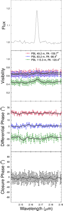
Figure 3: AMBER observation of VV Ser with three different baselines and spectral resolution R=1500. From top to bottom: Br$\gamma$ line profile (normalised to the continuum), visibilities, wavelength-dependent differential phases, and closure phase. A spectral binning to the raw data (from R=1500 to R=750) is overplotted in grey (solid line). For clarity, the differential phases of the shortest and longest baselines have been shifted by +20^o and -20^o.

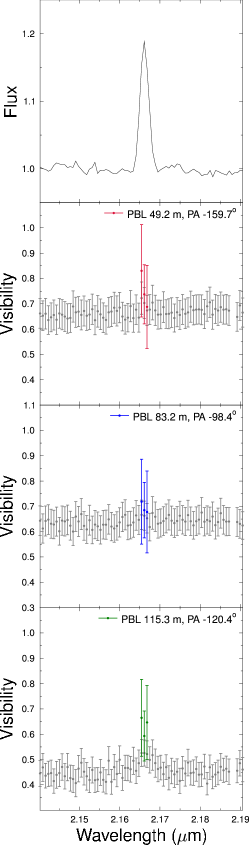
Figure 4: Observed AMBER pure Br$\gamma$ line visibilities of VV Ser. From top to bottom: wavelength dependence of flux, visibilities of the first, second, and third baseline. In each visibility panel the observed total visibilities (grey), and the observed continuum-compensated pure Br$\gamma$ line visibilities of each baseline (red, blue and green) are shown.

4.1 The size of the Br$\gamma$ emitting region

Our AMBER-MR observations of VV Ser allow us to measure the dispersed pure Br$\gamma$ line visibilities at three different radial velocities across the Br$\gamma$ line. To measure this continuum-compensated visibilities, we used the method described in Weigelt et al. (2007). According to this technique, within the wavelength region of the Br$\gamma$ line, the visibility has two components: the pure-line emitting component and the continuum emitting component. This latter includes contributions from both the circumstellar environment and the stellar component. Therefore, the emission line visibility $V_{Br\gamma}$ in each spectral channel can be written as $F_{{\rm Br}\gamma}V_{{\rm Br}\gamma}=|F_{\rm tot}V_{\rm tot}-F_{\rm c}V_{\rm c}|$ if the differential phase is zero (see Weigelt et al., 2007, for more details). The values $F_{\rm tot}$ and $V_{\rm tot}$ denote the total measured flux and visibilities in the Br$\gamma$ line, and $F_{\rm c}$ and $V_{\rm c}$ the continuum flux and visibility, respectively. This procedure takes then into account the contribution of the intrinsic photospheric absorption feature of VV Ser by considering a synthetic spectrum of the same spectral type and surface gravity (see, Table 5). The resulting pure Br$\gamma$ line visibilities are shown in Fig. 4. Only spectral channels with a line flux higher than 10 per cent of that of the continuum were considered.

The average line visibilities are 0.75, 0.70, and 0.65 for the shortest ($\sim$50 m), medium ($\sim$83 m) and longest ($\sim$115 m) baseline, respectively. Similarly to the continuum fitting, an approximate size of the Br$\gamma$ line emitting can be derived from the pure line visibility values.

5 Modelling spectroscopic and interferometric observations

To constrain the physical processes dominating VV Ser circumstellar environment, we model the emission line profiles obtained with LBT-LUCIFER (Section 3) and the VLTI-AMBER interferometric data (e.g. visibility and differential phases; Section 4).

To model the line profiles, we use the radiative transfer code torus (e.g. Harries 2000; Symington et al. 2005; Kurosawa et al. 2006; Kurosawa et al. 2011). In particular, the numerical method used in the current work is essentially identical to that in Kurosawa et al. (2011), originally developed to study CTTSs. The model employs the adaptive mesh refinement grid in Cartesian coordinate and assumes an axisymmetry around the stellar rotation axis. The model includes 20 energy levels of the hydrogen atom. The non-local thermodynamic equilibrium (non-LTE) level populations are computed using the Sobolev approximation (e.g. Sobolev, 1957; Castor, 1970; Castor & Lamers, 1979). For more comprehensive descriptions of the code, readers are referred to Kurosawa et al. (2011).

For the work presented here, three minor modifications have been, however, introduced in the code described in Kurosawa et al. (2011). Firstly, the model now includes continuum emission from a geometrically narrow ring which emulates the K-band dust emission near the dust sublimation radius. This emission contribution is important for modelling a correct line strength of the Br$\gamma$ line as well as the interferometric quantities around the line.

Secondly, the effect of a rotating magnetosphere has been included using the method described in Muzerolle et al. (2001). Until now, the code has been applied only to CTTSs. These stars are slow rotators, with rotation periods of 2–10 d (e.g. Herbst et al. 1987; Herbst et al. 1994). Hence, the effect of the rotation in CTTSs are small/negligible (e.g. Muzerolle et al. 2001). Conversely, intermediate-mass Herbig Ae/Be stars are expected to be fast rotators with periods of $0.2$ to a few days (e.g. Hubrig et al., 2009, 2011). Therefore, the effect of rotation should be included for modelling VV Ser.

Thirdly, the code has been modified to write model intensity maps as a function of wavelength (or velocity bins). This will allow us to compute the interferometric quantities, such as visibility, differential and closure phases, as a function of wavelength, which can be then directly compared with the spectro-interferometric observations of VLTI-AMBER.

The difference in the rotation properties of CTTSs and Herbig AeBe stars could be due the weak magnetic fields detected in Herbig AeBe stars. Indeed, spectro-polarimetric surveys of Herbig AeBe stars recently revealed the presence of weak magnetic fields in these sources, although much weaker than those measured in CTTSs (from few to several hundreds of Gauss vs. the some kG measured in CTTSs; Hubrig et al., 2009; Alecian et al., 2013). Additonal evidence of magnetic fields is given by the fact that many Herbig AeBe stars are also X-ray sources (Hubrig et al., 2009; Drake et al., 2014). As a consequence, the magnetic truncation radius of Herbig AeBe stars is expected to be located much closer to the protostar than in CTTSs (see, e.g. Shu et al., 1994; Muzerolle et al., 2004), giving rise to very compact, fast rotating, magnetospheres. This scenario is additionally supported by recent NIR and optical spectroscopic surveys of Herbig AeBe stars (see, e.g. Cauley & Johns-Krull, 2014, 2015; Fairlamb et al., 2015). In particular, these studies show clear evidences of inverse P-Cygni profiles in Herbig Ae and late type Herbig Be stars (indicative of accretion), as well as blue-shifted absorption features in strong accretors (indicative of accretion-driven outflows). These findings, along with the lack of inverse P-Cygni profiles in Herbig Be stars, suggest a general transition from magnetically controlled accretion in Herbig Ae and late type Be stars to boundery layer accretion in Herbig Be stars (see Cauley & Johns-Krull, 2015; Fairlamb et al., 2015).

For the particular case of VV Ser, attempts at measuring the magnetic field were firstly performed by Hubrig et al. (2009). This study, was however only capable of diagnosing VV Ser’s magnetic field at a significant level of 2.7$\sigma$ (200$\pm$75 G), and thus VV Ser was only classified as an Herbig star "suggestive" of the presence of a magnetic field. Additional attempts were performed by Alecian et al. (2013). In this case, a magnetic field of 561 G was measured, although with a large uncertainty of $\pm$238 G. The difficulty in measuring the magnetic field of VV Ser through spectro-polarimetry is probably due to the combination of the faintness of this source (V=11.6, and a nearly edge-on disc, self-shadowed by a puffed-up inner disc rim, see Pontoppidan et al. 2007), along with the large measurement uncertainties of this technique. However, VV Ser shows inverse P-Cygni profiles in several optical lines (see Mendigutía et al., 2011; Cauley & Johns-Krull, 2015), as well as redshifted absorption components in the Pa$\delta$ and Br$\gamma$ lines observed in our LBT NIR spectra (see Fig. 1). For these reasons, there is the possibility that VV Ser is weakly magnetised and has a compact magnetosphere and an accretion driven wind. Therefore, in the following sections we explore this possibility, and further assume that the outflow mechanisms in VV Ser are similar to those in the CTTSs which are also magnetised but have stronger magnetic fields. In particular, we examine our spectroscopic and interferometric data using combinations of a magnetosphere, a disc wind and a bipolar wind.

Finally, it is worth noting that the advantages of the adopted model over a simple geometric model are several. Firstly, our modelling can provide us with estimates of basic physical parameters under our assumptions, such as the wind mass-loss rate, the gas temperature and density, in addition to the emission geometry. Secondly, it allows us to model the emission lines observed with LBT (Pa$\delta$, Pa$\beta$, and Br$\gamma$) simultaneously, and in a self-consistent way.

5.1 Model configurations

Our model sketches are shown in Fig. 5. The three models consider three distinct flow components: (1) a dipolar magnetospheric accretion zone (magnetosphere) as described in Hartmann et al. (1994) and Muzerolle et al. (2001), (2) a disc wind emerging from the equatorial plane (a geometrically thin accretion disc) located outside of the magnetosphere (Fig. 5, left) and (3) a bipolar outflow in the polar regions of the star (Fig. 5, right). In the following, we briefly describe each flow component and their key parameters. Detailed descriptions of each component can be found in Kurosawa et al. (2011).

5.1.1 Magnetosphere

The accretion stream through a dipolar magnetic field is described as $r=R_{\mathrm{m}}\,\sin^{2}{\theta}$ (e.g. Ghosh et al. 1977; Ghosh & Lamb 1979; Hartmann et al. 1994) where $r$ and $\theta$ are the polar coordinates; $R_{\mathrm{m}}$ is the magnetospheric radius at the equatorial plane. The accretion funnel regions are defined by two stream lines corresponding to the inner and outer magnetospheric radii, that is, $R_{\mathrm{m}}=R_{\mathrm{mi}}$ and $R_{\mathrm{mo}}$ (Fig. 5). We adopt the density and temperature structures along the stream lines as in Muzerolle et al. (2001). The temperature scale is normalised with a parameter $T_{\mathrm{m}}$ which sets the maximum temperature in the stream. The mass-accretion rate $\dot{M}_{\mathrm{a}}$ scales the density of the magnetospheric accretion funnels.

5.1.2 Disc wind

Our disc wind model is an adaptation of the “split-monopole” wind model by Knigge et al. (1995) and Long & Knigge (2002). This simple kinematic wind model roughly follows the basic ideas of the magneto-centrifugal wind paradigm (e.g. Blandford & Payne 1982). The outflow arises from the surface of the rotating accretion disc, and has a biconical geometry. The specific angular momentum is assumed to be conserved along stream lines, and the poloidal velocity component is assumed to be simply radial from “sources” vertically displaced from the central star. Near the disc surface where the wind emerges, the value of the velocity toroidal component is similar to that of the local Keplerian velocity of the disc.

Table 5: Adopted parameters of the star and magnetosphere for VV Ser

$R_{*}$	$M_{*}$	$T_{\mathrm{eff}}$	$\log g$	$P_{*}$	$d$	$\dot{M}_{\mathrm{a}}$	$R_{\mathrm{mi}}$	$R_{\mathrm{mo}}$	$T_{\mathrm{m}}$
($\mathrm{R_{\odot}}$)	($\mathrm{M_{\odot}}$)	($\mathrm{K}$)	(cgs)	(d)	($\mathrm{pc}$)	($\mathrm{M_{\odot}yr^{-1}}$)	($R_{*}$)	($R_{*}$)	($\mathrm{K}$)
$2.6$	$4.0$	$14000$	$4.0$	$0.86$	$415$	$3.3\times 10^{-7}$	$1.3$	$1.8$	$10000$

Our model has five basic parameters: (1) the total mass-loss rate in the disc wind ($\dot{M}_{\mathrm{dw}}$), (2) the degree of the wind collimation, (3) the steepness of the radial velocity ($\beta_{\mathrm{dw}}$), (4) the wind temperature, and (5) the power-law index of the local mass-loss rate per unit area $\dot{m}(w)\propto w^{-p}$ where $w$ is the distance from the star on the equatorial plane. The basic configuration of the disc-wind model is shown in Fig. 5. The disc wind originates from the disc surface, and the “source” points ($S$), from which the stream lines diverge, are placed at a distance $D$ above and below the centre of the star. The angle at which the matter is launched from the disc is controlled by changing the value of $D$. The mass-loss launching occurs between $R_{\mathrm{wi}}$ and $R_{\mathrm{wo}}$ where the former is set to be near the outer radius of the closed magnetosphere ($R_{\mathrm{mo}}$) and the latter to be a free parameter. The wind density is normalised with the total mass-loss rate in the disc wind ($\dot{M}_{\mathrm{dw}}$). The temperature of the wind ($T_{\mathrm{dw}}$) is assumed as isothermal.

Table 6: Model parameters for disc wind and bipolar outflow.

	MA†		Disc wind								Bipolar outflow
	(1)		(2)	(3)	(4)	(5)	(6)	(7)	(8)		(9)	(10)	(11)	(12)	(13)	(14)
			$\dot{M}_{\mathrm{dw}}$	$R_{\mathrm{wi}}$	$R_{\mathrm{wo}}$	$p$	$T_{\mathrm{dw}}$	$\beta_{\mathrm{dw}}$	$D$		$\dot{M}_{\mathrm{bp}}$	$\theta_{\mathrm{bp}}$	$R_{0}$	$T_{\mathrm{bp}}$	$V_{\infty}$	$\beta_{\mathrm{bp}}$
Model			($\mathrm{M_{\odot}yr^{-1}}$)	($R_{*}$)	($R_{*}$)	$\cdots$	($\mathrm{K}$)	$\cdots$	($R_{*}$)		($\mathrm{M_{\odot}yr^{-1}}$)	$\cdots$	($R_{*}$)	($\mathrm{K}$)	($\mathrm{km\,s^{-1}}$)	$\cdots$
A∗	yes		$\cdots$	$\cdots$	$\cdots$	$\cdots$	$\cdots$	$\cdots$	$\cdots$		$\cdots$	$\cdots$	$\cdots$	$\cdots$	$\cdots$	$\cdots$
B	yes		$3\times 10^{-8}$	$1.8$	$10.0$	$2.3$	$10^{4}$	$4.0$	$2.2$		$\cdots$	$\cdots$	$\cdots$	$\cdots$	$\cdots$	$\cdots$
C	no		$3\times 10^{-8}$	$1.8$	$10.0$	$2.3$	$10^{4}$	$4.0$	$2.2$		$\cdots$	$\cdots$	$\cdots$	$\cdots$	$\cdots$	$\cdots$
D	yes		$3\times 10^{-8}$	$5.8$	$14.0$	$2.3$	$10^{4}$	$4.0$	$2.2$		$\cdots$	$\cdots$	$\cdots$	$\cdots$	$\cdots$	$\cdots$
E	yes		$4\times 10^{-8}$	$3.8$	$12.0$	$0.2$	$10^{4}$	$2.0$	$2.2$		$\cdots$	$\cdots$	$\cdots$	$\cdots$	$\cdots$	$\cdots$
F	yes		$\cdots$	$\cdots$	$\cdots$	$\cdots$	$\cdots$	$\cdots$	$\cdots$		$6\times 10^{-8}$	$35^{\circ}$	$2.4$	$10^{4}$	$500$	$1.2$
G	no		$\cdots$	$\cdots$	$\cdots$	$\cdots$	$\cdots$	$\cdots$	$\cdots$		$6\times 10^{-8}$	$35^{\circ}$	$2.4$	$10^{4}$	$500$	$1.2$

Note: ($\dagger$) MA indicates if a model includes a magnetospheric accretion. If indicated by ‘yes’, the parameters in Table 5 are used for the magnetosphere. (*) Model A consists of the magnetospheric accretion flows only.

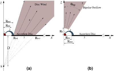
Figure 5: Basic model configurations of the circumstellar flows which consist of (a) a magnetosphere and a disc wind (left panel), or (b) a magnetosphere and a bipolar outflow (right panel). The density is assumed to be axisymmetric and top-down symmetric. The components of the models are: (1) the continuum source (star) located at the origin of the cartesian coordinates system, (2) the magnetospheric accretion flow, (3) the geometrically thin accretion disc, (4) the disc wind, and (5) the bipolar outflow. The split-monopole (with the source displacement distance $D$) disc wind emerges from the equatorial plane, but only within the distances from $z$-axis between $R_{\mathrm{wi}}$ and $R_{\mathrm{wo}}$. The bipolar outflow is launched from a sphere with radius $R_{\mathrm{0}}$, but is restricted within the cones with the half opening angle $\theta_{\mathrm{bp}}$. The figure is not to scale.

5.1.3 Bipolar outflow

As an alternative flow geometry, we also consider a bipolar outflow which arises in the polar regions near the star. Possible scenarios in which this type of outflows could occur are: (1) an accretion-powered stellar wind launched from open magnetic field lines anchored to the stellar surface (e.g. Decampli 1981; Strafella et al. 1998; Bouret & Catala 2000; Matt & Pudritz 2005; Cranmer 2008, 2009), or (2) a relatively fast magnetically driven polar outflow which appears in between the slower conically-shaped winds launched from the disk-magnetosphere interaction regions (e.g. Romanova et al. 2009; Lii et al. 2012).

The bipolar outflow is approximated as an outflow consisting of narrow cones with a half-opening angle $\theta_{\mathrm{bp}}$. Here, we assume that the flow propagates only in the radial direction, and that its velocity is described by the classical beta-velocity law (cf. Castor & Lamers 1979):

$$v_{r}\left(r\right)=v_{0}+\left(v_{\infty}-v_{0}\right)\left(1-\frac{R_{0}}{r}\right)^{\beta_{\mathrm{bp}}}\,,$$ (3)

where $v_{\infty}$ and $v_{0}$ are the terminal velocity and the velocity of the outflow at the base ($r=R_{0}$). Here, we set $v_{0}=10\,\mathrm{km\,s^{-1}}$ which roughly corresponds to the thermal velocity of gas around $10^{4}$ K.

Assuming that the mass-loss rate of the outflow is $\dot{M}_{\mathrm{bp}}$ and following the mass-flux conservation in the flows, the density $\rho_{\mathrm{pb}}$ of the outflow can be written as:

$$\rho_{\mathrm{bp}}\left(r\right)=\frac{\dot{M}_{\mathrm{bp}}}{4\pi r^{2}v_{r}\left(r\right)\left(1-\cos\theta_{\mathrm{bp}}\right)}\,.$$ (4)

The temperature of the bipolar outflow ($T_{\mathrm{bp}}$) is assumed isothermal as in Kurosawa et al. (2011). To avoid an overlapping of the bipolar outflow with the accretion funnels, the base of the bipolar outflow ($R_{0}$) is set approximately at the outer radius of the magnetosphere ($R_{\mathrm{mo}}$) (cf. Fig. 5). The rotational velocity of the flow is assigned such that the specific angular momentum of gas is conserved along the stream lines, and its initial value is constrained by the rotation speed of the stellar surface. A similar bipolar outflow model was recently applied to the pre-FUor star, V1331 Cyg (Petrov et al., 2014).

The bipolar outflow introduced here is rather a simple kinematic model which does not involve a physical mechanism for the wind acceleration. However, since the outflow geometry here is drastically different from that of a disc wind model, it is useful to consider this model to qualitatively check if the outflow in VV Ser arises mainly from the polar regions or the accretion disc.

5.2 Modelling line profiles

In this section, we will apply the models described above (i.e. magnetospheric accretion, disc wind and bipolar outflow) to model the H i line profiles obtained from the LBT observations. Due to the complex line profiles and line variability observed in these data, we opted to model, as a first approximation, the average line profiles of the Br$\gamma$, Pa$\beta$ and Pa$\delta$ lines during the three epochs. These data offer a higher spectral resolution (R$\sim$7000) than the MR-AMBER data (R$\sim$1500). The origin of the line variability will be discussed in Section 6.

5.2.1 Adopted stellar and disc parameters

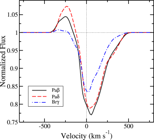
Figure 6: Pa$\beta$ (solid), Pa$\delta$ (dash) and Br$\gamma$ (dash-dot) model line profiles for VV Ser computed (at $i=70^{\circ})$ with a small magnetosphere with $R_{\mathrm{mi}}=1.3\,R_{*}$ and $R_{\mathrm{mo}}=1.8\,R_{*}$ and the stellar rotation period of $P_{*}=0.84$ d. Other model parameters are summarised in Table 5. The lines are mainly in absorption except for a very small emission component that arises on the blue side of the profiles. The model profiles clearly disagree with the observed profiles which display instead a relatively strong emission peak around the line centres (Fig. 1). For clarity, the continuum emission from the ring emission around the dust sublimation radius and photospheric absorption are excluded in these models.

The basic stellar parameters adopted for modelling the VV Ser spectra from the LBT are listed in Table 5. The atmosphere model of Kurucz (1979) with $T_{\mathrm{eff}}=14000$ K and $\log g=4.0$ (cgs) is used as the source of the stellar continuum in the line radiative transfer models. A disk inclination angle $i$ of $\sim$70° is assumed (Pontoppidan et al., 2007; Eisner et al., 2014). The speed at which the star rotates at the equator ($v_{\mathrm{eq}}$) was estimated assuming that the disc/ring normal vector coincides with the rotation axis of VV Ser, and that $v_{\mathrm{eq}}$ is the same as $v$ in $v\sin i$. In the case of VV Ser, $v\sin i=142\,\mathrm{km\,s^{-1}}$ (Vieira et al. 2003), and thus $v_{\mathrm{eq}}=151\,\mathrm{km\,s^{-1}}$ (approximately $0.3$ of the breakup velocity). Consequently, the rotation period of VV Ser is estimated to be $P_{*}=2\pi R_{*}/v_{\mathrm{eq}}=0.86$ d. This value is in agreement with the one estimated by Hubrig et al. (2009). Finally, a mass-accretion rate of 3.3$\times$10^-7 M_⊙ yr^-1is assumed.

To model the dust disc of VV Ser, a uniform geometrical ring model is used to fit the AMBER continuum visibility data in Section 4. The inner radius of the ring is estimated to be 2.35 mas which corresponds to 0.97 au at $d=415$ pc. We adopt the same ring geometry and dimensions as in the line profile calculations. We also adopt the position angle (PA) and the ring inclination angle ($i$) from our earlier analysis (Table 4), i.e. PA= 66$\aas@@fstack{\circ}$7 and $i$=70°, respectively. The ring is assumed to emit as a blackbody at a temperature $T_{\mathrm{ring}}=1400$ K.

5.2.2 Line profiles from magnetospheric accretion models

In this section, we briefly discuss the effect of magnetospheric accretion (see Section 5.1.1) on the formation of the NIR atomic hydrogen emission lines observed in VV Ser. Using the stellar parameters listed in Table 5, the corotation radius ($R_{\mathrm{cr}}$) of VV Ser becomes $R_{\mathrm{cr}}=\left(GM_{*}\right)^{1/3}\left(P_{*}/2\pi\right)^{2/3}=2.4\,R_{*}$. We assume that the extent of the magnetosphere is slightly smaller than $R_{\mathrm{cr}}$, and set the inner and outer radii of the magnetospheric accretion funnel to be $R_{\mathrm{mi}}=1.3\,R_{*}$ and $R_{\mathrm{mo}}=1.8\,R_{*}$. These radii (in the units of the stellar radius) are considerably smaller than those of CTTSs (e.g. Königl 1991; Muzerolle et al. 2004). Consequently, the volume of the gas emitting region/accretion funnel becomes very small. Hence, the hydrogen line emission strengths are expected to be also very small. The weakness of emission lines in the small and fast-rotating magnetosphere was first pointed out by Muzerolle et al. (2004), in modelling the Balmer lines of Herbig Ae star UX Ori (see their fig. 3).

Figure 6 shows the Pa$\beta$, Pa$\delta$ and Br$\gamma$ model line profiles assuming that they are only formed in the magnetosphere. As expected, the lines are rather weak, and mainly in absorption except for a very small emission component on the blue side of the profiles. Very similar line shapes are also found in the rotating magnetosphere model of Muzerolle et al. (2004) (their fig. 3). The model clearly disagrees with the observed line profiles (Fig. 1) which display strong emission peaks around the line centres. In particular, the observed Pa$\beta$ and Br$\gamma$ emission lines are roughly symmetric around the line centres.

Although not shown here, we have computed models with various combinations of magnetospheric temperature $T_{\mathrm{m}}$ and mass-accretion rates ($\dot{M}_{\mathrm{a}}$). The line shapes of those models are similar to those shown in Fig. 6. In general, the symmetric, or almost symmetric, emission line profiles are difficult to explain with a fast-rotating magnetosphere model alone, especially at a high inclination angle, as in VV Ser. For this reason, it is most likely that an additional gas flow component is involved in the formation of the hydrogen emission lines.

It must be noted, however, that the results presented here may not apply to other Herbig Ae/Be stars. To examine whether the results above are applicable to Herbig Ae/Be stars in general, a further investigation is needed. For instance, one would need to explore much larger parameter spaces. However, this is beyond the scope of the present paper and shall be investigated in the future.

5.2.3 Line profiles from disc wind models

To overcome the weakness of the line emission in the models with a magnetospheric accretion funnel (Fig. 6), an additional emission volume from a disc wind (see Section 5.1.2) will be added to the magnetospheric contribution.

The left panels in Fig. 8 show the model line profiles, computed at $i=70^{\circ}$ (i.e. almost edge-on), resulting from the combination of a magnetospheric accretion funnel and a disc wind (Model B). The main model parameters are summarised in Table 6. The ratio of the wind mass-loss rate to the mass-accretion rate ($\dot{M}_{\mathrm{dw}}/\dot{M}_{\mathrm{a}}$) is $\sim 0.09$. This model produces similar line strengths and widths as seen in the observed Pa$\beta$, Pa$\delta$ and Br$\gamma$ lines of the LBT observations. However, the model profiles clearly disagree with the observed profiles in their shapes: the former are double-peaked, but the latter are single-peaked. This is because in our disc wind model the H i NIR lines are mainly formed near the base of the disc wind. In this region the Keplerian rotation of the wind dominates over the radial motion. Therefore, double-peaked profiles naturally occur when the disc wind is viewed from horizontal directions, that is, when the system has a mid to high inclination angle ($i$). This is demonstrated in Fig. 7, which shows how the Br$\gamma$ line profile depends on the inclination angle. In particular, this figure shows that the modelled Br$\gamma$ line profile becomes double peaked for $i\mathrel{\hbox{\raise 2.15277pt\hbox{$>$}\hbox to0.0pt{\hss\lower 2.15277pt\hbox{$\sim$}}}}30^{\circ}$. Note that in our disc wind model, the Keplerian velocities are about $400\,\mathrm{km\,s^{-1}}$ and $170\,\mathrm{km\,s^{-1}}$ at the inner and outer radii of the wind launching regions, that is, $R=1.8\,\mathrm{R_{\odot}}$ and $10\,\mathrm{R_{\odot}}$, respectively. Moreover, the line emission mainly originates from the disc wind and the contribution of the magnetosphere to the line profile is very small (see Section 5.2.2). This is illustrated in the right panels of Fig. 8, where a comparison of the line profiles produced by the magnetosphere plus disc wind model (Model B), with those generated by the single contributions of the disc wind model (Model C), and the magnetosphere model (Model A) is shown. Therefore, in model B (magnetosphere + disc wind), the overall shape of the H i lines is dominated by the emission from the disc wind.

Although not shown here, we have explored various combinations of the disc wind model parameters (i.e. $\dot{M_{\mathrm{dw}}}$, $R_{\mathrm{wi}}$, $R_{\mathrm{wo}}$, $D$, $T_{\mathrm{dw}}$ $\beta_{\mathrm{dw}}$ and $p$ as in Section 5.1.2; see also Fig. 5) which control the characteristics of the wind. Examples of the dependency of the Br$\gamma$ profile on a few selected models parameters (the wind launching radii $R_{\mathrm{wi}}$ and $R_{\mathrm{wo}}$; the power-law index of local mass-loss rate per unit area $p$) are given in Appendix A. Even though the line strengths, line widths and the peak separation widths vary with different combinations of the disc wind parameters, the double peaks are always visible for a mid to high inclination angle, as is the case for VV Ser (assuming $i\approx 70^{\circ}$). Hence, the disc wind is unlikely a major contributor to the single-peaked emission lines (Pa$\beta$, Pa$\delta$ and Br$\gamma$) seen in VV Ser. However, if the inclination is $\sim$70° or larger, we cannot exclude the possibility that the innermost region of the disc wind is obscured by the outer region of a flared disc, and thus that another flux contribution is dominant. For these reasons, we seek an alternative flow component which can robustly reproduce a rather symmetric and single-peak Br$\gamma$ emission line as seen in VV Ser and many other Herbig Ae/Be stars (e.g. Garcia Lopez et al. 2006; Brittain et al. 2007). Note that, for a relatively low inclination angle system (nearly face-on), it may be still possible to reproduce a single peaked Br$\gamma$ by a disc wind model (e.g. Fig. 7; see also Weigelt et al. 2011; Garcia Lopez et al. 2015; Caratti o Garatti et al. 2015).

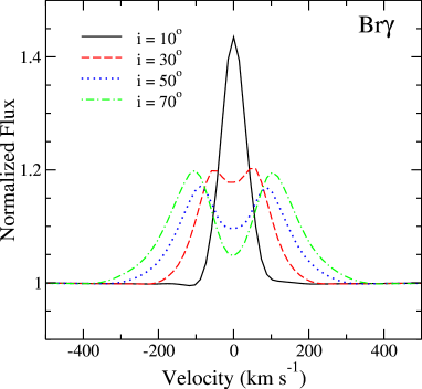
Figure 7: The dependency of Br$\gamma$ on inclination angle ($i$) in Model B which uses a combination of a disc wind and magnetosphere (Table 6). The line profiles are double-peaked for the models with $i\mathrel{\hbox{\raise 2.15277pt\hbox{$>$}\hbox to0.0pt{\hss\lower 2.15277pt\hbox{$\sim$}}}}30^{\circ}$. Disc models in general have difficulties reproducing the singe-peak Br$\gamma$ line profile seen in the LBT observations (Fig.1) for the models with mid to high inclination angles.

5.2.4 Line profiles from bipolar outflow models

Another possible way to obtain a single-peak emission line profile in a nearly edge-on system is to include a bipolar outflow in the model. In this case, the inclination angle $i$ must be larger than the half-opening angle of the bipolar outflow $\theta_{\mathrm{bp}}$ (see Fig. 5) to avoid a strong wind absorption on the blue side of the line profile (i.e. a P-Cygni profile).

The left panels in Fig. 9 shows the model line profiles computed with a combination of a magnetospheric accretion funnel and a bipolar outflow (Model F). The lines are computed at $i=70^{\circ}$ assuming a wind half-opening angle $\theta_{\mathrm{bp}}=35^{\circ}$. The model parameters are summarised in Table 6. The ratio of the mass-loss rate in the wind to the mass-accretion rate ($\dot{M}_{\mathrm{dw}}/\dot{M}_{\mathrm{a}}$) is about $0.18$. The figure clearly shows that the model is capable of producing single-peak line profiles. Furthermore, the model produces line profiles very similar to the observed Pa$\beta$, Pa$\delta$ and Br$\gamma$ line profiles (in their line strengths and widths).

As for the case of the magnetosphere-plus-disc wind model, the line emissions in this model are mainly from the bipolar outflow. This is clearly illustrated in the right panels of Fig. 9, which compare the profiles from Model F (magnetosphere + bipolar outflow) with those computed with only the bipolar outflow (Model G) and only the magnetosphere (Model A). In this particular model (Model F), the magnetosphere contributes only slightly to the lines, and the overall shapes of the lines are determined by the emission from the bipolar outflow.

The emission profiles of the Pa$\beta$ and Br$\gamma$ lines are mostly symmetric around the line centres. However, the Pa$\delta$ line profile is slightly asymmetric towards the blue side of the line, that is, the blue-shifted emission is slightly stronger. This is due to the absorption by the magnetospheric accretion funnel which is stronger on the red side of the line. A similar trend is also observed in the Pa$\delta$ line computed with the disc wind + magnetosphere (Model B) in Fig. 8, which shows stronger blue-shifted emission.

In summary, the bipolar outflow, when viewed from equatorial directions, can form single-peak line profiles as the ones observed in the LBT spectra. The line strengths and shapes of the observed Pa$\beta$, Pa$\delta$ and Br$\gamma$ line profiles are reproduced well by Model F (Fig. 9; Table 6).

5.3 Models for AMBER data

To probe whether the same bipolar outflow plus magnetosphere model described above can reproduce the Br$\gamma$ AMBER-VLTI spectro-interferometric observations (Section 4) in addition to the LBT spectra, the intensity maps of the line emitting regions were computed using the same radiative transfer model employed to produce the line profiles (see Section 5). In this way, the interferometric quantities such as visibility, differential and closure phases can be readily calculated from the model intensity maps.

The results are summarised in Fig. 10. The figure compares the model Br$\gamma$ line profiles, visibility and differential phases with those of LBT (average Br$\gamma$ line profile) and VLTI-AMBER observations. For purposes of comparison, the figure also includes the models computed with a disc wind plus a magnetosphere in addition to those with the bipolar outflow. Six different cases in Table 6 are shown here: (1) a disc wind with small launching radii (Model B) computed at $i=70^{\circ}$, (2) a disc wind with larger launching radii (Model D) computed at $i=70^{\circ}$, (3) a disc wind with intermediate launching radii and a small $p$ (the index of the power-law in the mass-loss rate per unit area; see Appendix A and Kurosawa et al. 2011) (Model E) computed at $i=70^{\circ}$, (4) a bipolar outflow model (Model F) computed at $i=65^{\circ}$, (5) same as (4) but computed at $i=70^{\circ}$, and (6) same as (4) but with $i=75^{\circ}$. Note that model closure phases are not shown in this figure because no closure-phase signal within the error of $20^{\circ}$ is measured from our AMBER observations (see, Fig. 3), and all model closure phases are smaller than 10°.

In cases (1)–(3) (disc wind models), the models fit the interferometric observations reasonably well. However, the double-peak line profiles seen in those models do not match the observations. The separation of the double peaks are slightly reduced by increasing the disc wind launching radii from case (1) (Model B) to case (2) (Model D) (Table 6). A further reduction of the peak separation is achieved by reducing the value of $p$ (the power-law for the mass-loss rate per unit area; c.f. Appendix A; Kurosawa et al. 2011) from case (2) (Model D) to case (3) (Model E) (Table 6). The double-peak feature is rather persistent in the models with a disc wind (see Section 5.2.3). On the other hand, the bipolar outflow models (Model F) with $i=65^{\circ}$ (case 4) and $75^{\circ}$ (case 6) reproduce reasonably well the observed line profiles, but the visibility levels disagree with the AMBER observations. Only the model with the bipolar outflow computed at $i=70^{\circ}$, case (5), fits the observed line profiles (here and also in Fig. 9), visibility and differential phase, simultaneously.

In all the models, the visibility levels are slightly larger in the lines (by $\sim 0.06$) compared to those in the continuum. This agrees with the fact that the line emitting regions are smaller than that of the continuum emitting regions. In our models, the inner radius of the K-band continuum emitting ring model is approximately 1.0 au (Section 4.1) which corresponds to $\sim 80\,\mathrm{R_{\odot}}$. This is much larger than the wind launching regions of both disc wind ($1.8$–$14\,\mathrm{R_{\odot}}$) and bipolar outflow ($2.4\,\mathrm{R_{\odot}}$) (Table 6). The increase in the visibility levels across the Br$\gamma$ emission line is not clearly seen in the AMBER observations due to the relatively low S/N and spectral resolution of the data. However, a weak increase of the visibility at the longest baseline (UT1–UT4) is observed towards the line centre (see Fig. 3). The small increase in the visibility in the line centre ($\sim 0.06$) with respect to the continuum seems to be in agreement with the data, considering the levels of uncertainty/noise.

The differential phases from the AMBER observation are $0^{\circ}$ within the error of $5^{\circ}$ across the Br$\gamma$ line without any trend for an increase or a decrease. On the other hand, our models show very small variations with their amplitude between $\sim 1^{\circ}$ and $\sim 2^{\circ}$ across the line. These small amplitudes are well below the noise levels of the observations. This suggests that the models do not disagree with the observed differential phases, that is, the amplitude of the variation in the differential phase across the line predicted by the model do not exceed the noise levels in the observations.

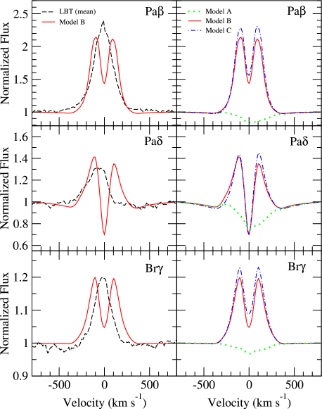
Figure 8: Left Panels: a comparison of the mean line profiles obtained by LBT (dashed) with the hydrogen line profiles (Pa$\beta$, Pa$\delta$ and Br$\gamma$) computed using the models with the combination of a disc wind and magnetosphere (solid; Model B in Table 6). Right panels: a comparison of line profiles computed using the disc wind + magnetosphere (solid; Model B) with those using (1) only the disc wind (dash-dot; Model C) and (2) only the magnetosphere (dot; Model A). All the profiles are computed at the inclination angle $i=70^{\circ}$. In general, models with disc wind produced double-peak profiles due to rotating motion of the disc wind. The double peaks are always prominent at a mid to a high inclination angle (cf. Fig. 7). The right panels show that the emission contribution from the magnetosphere is very small in Model B.

In principle, the physical parameters of the line emitting wind regions (the wind geometry and kinematics) can be further constrained by performing detail model fitting of the observed visibility and differential phases across the line. However, the high noise levels in the data prevent us from performing such an investigation.

In summary, the model with a bipolar outflow (Model F) observed at an inclination angle of $i=70^{\circ}$ (the third column in Fig. 10) gives the best match to the observed visibility, differential phases and the NIR hydrogen line profiles (Pa$\beta$, Pa$\delta$ and Br$\gamma$ as in Fig. 9).

6 Discussion

6.1 Origin of the NIR H i emission lines

In the previous sections, we investigated possible mechanisms responsible for the formation of the NIR H i emission lines in the Herbig star VV Ser. With this goal in mind, we explored what should be expected from three different line emitting sources namely, a magnetosphere, a disc wind and a bipolar outflow, and compare these results with average H i line profiles obtained with LUCIFER at LBT, and with AMBER-MR spectro-interferometric observations. Our modelling suggests, that in the case of VV Ser, the contribution of a fast rotating magnetosphere to the H i NIR emission line profiles is very small in comparison with the contribution of a disc wind or bipolar outflow. Similar results have been previously found in other Herbig AeBe stars by analysing their NIR line profiles alone or in combination with NIR spectro-interferometric techniques (Weigelt et al., 2011; Tambovtseva et al., 2014; Garcia Lopez et al., 2015; Caratti o Garatti et al., 2015). In contrast with these results, where a disc wind model could be used to model the Br$\gamma$ line profile and the spectro-interferometric observables, in the case of VV Ser only a bipolar outflow can approximately reproduce the averaged single-peaked line profiles of the Pa$\beta$, Pa$\delta$, and Br$\gamma$ lines observed with the LBT, as well as, the Br$\gamma$ spectro-interferometric observables. The main difference, between VV Ser and the results mentioned above is the high disc inclination angle of VV Ser ($i\sim$70°). As shown in Fig. 7, our disc wind model can only reproduce single peaked line profiles when low inclination angles ($i\lesssim$30°) are considered. Similar results are also found in Tambovtseva et al. (2014) for the Br$\gamma$ and H$\alpha$ lines. This is because, the NIR H i lines are formed at the base of the disc wind, where the Keplerian rotation of the disc dominates over the wind radial velocity. Therefore, a disc wind can only generate a single peaked line profile at high inclination angles if the inner disc wind emitting region is obscured by an outer flared disc, or alternatively, if other components (such as a magnetosphere or a bipolar wind) significantly contribute to the line profile. In contrast, bipolar outflows are launched well above the circumstellar disc (see, sketch in Fig. 5), and thus, single peaked line profiles are easily obtained for all the NIR H i observed lines.

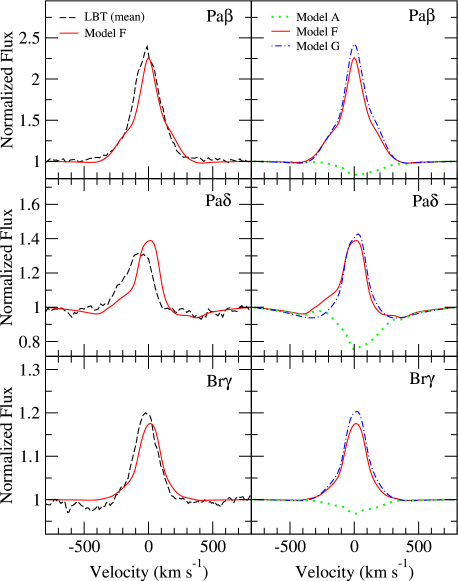
Figure 9: Left Panels: a comparison of the mean line profiles obtained by the LBT (dashed; see Section 3 and Fig. 1) with the model hydrogen line profiles (Pa$\beta$, Pa$\delta$ and Br$\gamma$) computed using the models with the combination of a bipolar outflow and magnetosphere (solid; Model F in Table 6). Right panels: a comparison of the line profiles computed using the bipolar outflow + magnetosphere (solid; Model F) with those using (1) only the bipolar outflow (dash-dot; Model G) and (2) only the magnetosphere (dot; Model A). All the profiles are computed at the inclination angle $i=70^{\circ}$. The left panels show that Model F can reasonably and simultaneously fit the observed Pa$\beta$, Pa$\delta$ and Br$\gamma$ profiles (mean) obtained by the LBT. The right panels show that the emission contribution from the magnetosphere is very small in Model F.

Although the bipolar outflow model works very well here, we would like to remind readers that the model is highly schematic, and the exact physical process which can produce this type of outflows is not well known. As mentioned earlier, one possible candidate is the accretion-powered stellar wind (e.g. Decampli 1981; Strafella et al. 1998; Bouret & Catala 2000; Matt & Pudritz 2005; Cranmer 2008, 2009); however, these models (except for Strafella et al. 1998; Bouret & Catala 2000) are mainly for winds in CTTSs which have stronger magnetic fields. Interestingly, recent spectroscopic studies of Herbig Ae/Be stars by Cauley & Johns-Krull (2014, 2015) have shown that about 30 per cent of their sample display P-Cygni profiles in HeI 10830 Å and H$\beta$, which is a good indication for stellar wind like outflows (e.g. Edwards et al. 2006; Kwan et al. 2007; Kurosawa et al. 2011).

Our AMBER-MR spectro-interferometric observations of the Br$\gamma$ line support the results obtained from the pure modelling of the LBT spectroscopic observations. That is, regardless of the accuracy on the line profile modelling, the wind (disc or bipolar wind) component dominates the line emission, whereas the magnetosphere do not play a major role in the line profile. Indeed, the AMBER-MR interferometric observations of the Br$\gamma$ line shows that even if the Br$\gamma$ line emission is more compact than the continuum emission, the Br$\gamma$ emission is nevertheless resolved. Therefore, the line emitting region is not mainly formed in the unresolved magnetospheric accretion region. Furthermore, the interferometric observables (visibilities, differential phases and closure phase) are best reproduced when a disc wind or bipolar outflow is considered, the latter being the one that best reproduces the Br$\gamma$ single line profile.

6.2 Line profile variability

As shown in Fig. 2, a significant fraction of the variation in the observed lines occurs in their red wings. Therefore, variations in the contribution of the magnetosphere to the total H i line emission could be the cause of the NIR H i line variability observed in VV Ser (see, Fig. 1). For instance, a periodic and a non-periodic line variability can be caused by rotating non-axisymmetric magnetospheric accretion flows in stable and unstable regimes, respectively (e.g. Kurosawa & Romanova 2013). Similarly, non-steady accretion or an enhanced mass-accretion rate could modify the redshifted component of the line profiles, introducing strong redshifted absorption components to the line profiles (see Fig. 6). This could be the cause of the redshifted adsorptions in the Pa$\delta$, Pa$\beta$ and Br$\gamma$ line profiles observed in February 2012 (see Fig. 1). On the other hand, the complex Pa$\delta$ line profile observed in April 2012 could be explained by an increase from a disc wind contribution to the line profile. A disc wind could also reproduce the double peaked H$\alpha$ line profiles observed in VV Ser (see e.g., Mendigutía et al. 2011). This might indicate that lines such as H$\alpha$ are optically thicker than the NIR H i emission lines. Furthermore, they are formed in regions located farther away from the disc plane and observed through the wind down to the central source. In this context, the complex line profiles and their variability could be explained through the coexistence of at least three different mechanisms, namely magnetospheric accretion, a disc wind and a bipolar outflow, the intensity and contribution to the total line profile of which vary with time. This would indicate that accretion, and thus, the ejection processes do not occur in a steady-state regime.

Non steady accretion has been previously used to explain the short term spectral and photometric variability of the CTTS AA Tau (Bouvier et al., 2003). In this case, the optical line profile and photometric variations were explained by the presence of a non-axisymmetric warp in the inner disc caused by the interaction of the disc and an inclined stellar dipole (e.g. Romanova et al. 2003, 2013). The variability is then related to the perturbation of the stellar magnetic field at the disc inner edge. In this regard, an increase in brightness, and the subsequent line variability, is due to a severe reduction of the accretion flow onto the star, leading to a temporary disappearance of the disc inner warp. However, it is not clear how such a mechanism could work in VV Ser. Whereas CTTSs are slow rotators as a consequence of strong magnetic fields producing a magnetic braking, Herbig AeBe stars are fast rotators with no clear evidence of a developed and organised magnetic field configuration (e.g., Hubrig et al., 2011, and references therein). Although the measured variations in the EW of the H i lines could be interpreted as changes in the continuum level (i.e. magnitude) of the source, they could also represented a decrease in the line flux. Therefore, without simultaneous photometry at both optical and NIR wavelengths it is difficult to test whether VV Ser’s variability is due to inner disc instabilities caused by enhanced/depressed accretion. Further observations, spanning a wider wavelength and temporal range, and accompanied by simultaneous optical and NIR photometry are needed in order to disentangle the inner disc mechanism producing the line variability.

7 Summary and conclusions

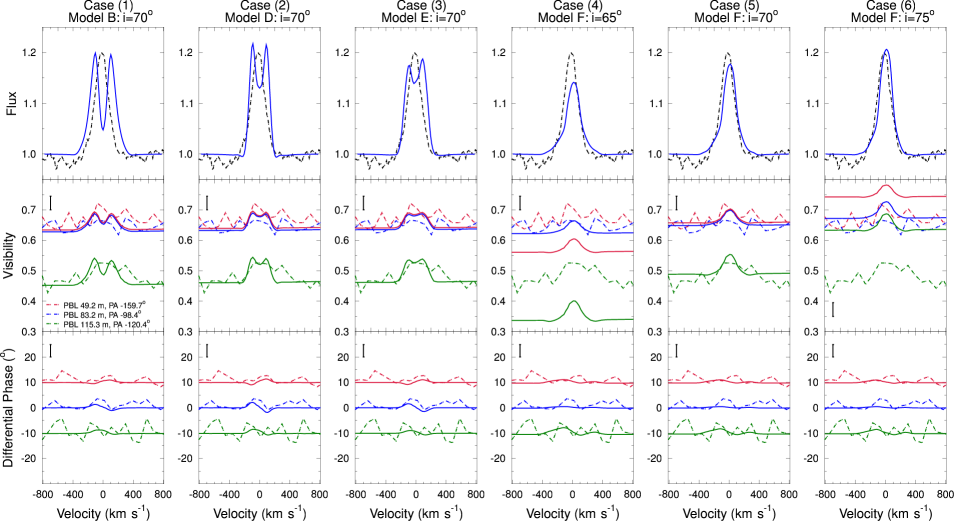
Figure 10: Comparisons of the LBT and AMBER observations of Br$\gamma$ with our models (six different cases): (1) Model B with $i=70^{\circ}$ — a disc wind with small launching radii (first column), (2) Model D with $i=70^{\circ}$ — a disc wind with lager launching radii (second column), (3) Model E with $i=70^{\circ}$ — a disc wind with intermediate launching radii and a small $p$ (third column), (4) Model F with $i=65^{\circ}$ — a bipolar outflow model (fourth column), (5) Model F with $i=70^{\circ}$ — a bipolar outflow model (fifth column), and (6) Model F with $i=75^{\circ}$ — a bipolar outflow model (sixth column). See Table 6 for their model parameters. The top panels show the comparisons of the mean Br$\gamma$ profile from the LBT (dash-dot) with models (solid). The middle and bottom panels show the comparisons of our models (solid) and the visibility and differential phases obtained by AMBER (Section 4) with three baselines: UT1–UT2 ($\mathrm{PBL}=49.20$ m, $\mathrm{PA}=-159.67^{\circ}$), UT2–UT4 ($\mathrm{PBL}=83.25$ m, $\mathrm{PA}=-98.40^{\circ}$) and UT1–UT4 ($\mathrm{PBL}=115.28$ m, $\mathrm{PA}=-120.38^{\circ}$). For clarity, the differential phases of UT2–UT4 and UT1–UT4 baselines are vertically shifted by $+10^{\circ}$ and $-10^{\circ}$, respectively. Model F with $i=70^{\circ}$ (fifth column) agrees reasonable well with the observed Br$\gamma$ profile, visibility and differential phase. The same model reproduces the observed Pa$\beta$ and Pa$\delta$ lines also well (Fig. 9). The disc wind models (Models B,D and E with $i=70^{\circ}$) fit the interferometric observations, but their line profile shapes (double peaked) do not match the observation. Although the bipolar outflow models (Model F) with $i=65^{\circ}$ and $75^{\circ}$ reproduce reasonably well the observed line profile, their visibility levels do not match with the observation.

We have shown LBT-LUCIFER medium resolution z-, J-, and K-band spectroscopic observations covering the Pa$\delta$, Pa$\beta$, and Br$\gamma$ lines of the Herbig star VV Ser at three different epochs spanning over three months. Additionally, MR VLTI-AMBER interferometric observations of the Br$\gamma$ line in this source are presented as well.

The spectroscopic observations show relatively strong line variability in all the H i NIR emission lines. The line profile variability is more extreme in the Paschen lines probably because the line emitting volume of these lines is larger than that of the Br$\gamma$ line. Therefore, an observer would receive emission originating from different circumstellar regions (such as a wind and magnetospheric region) along the line of sight. To investigate the physical mechanisms that are responsible for the H i line emission, we have a applied a radiative transfer model consisting of a magnetospheric accretion region, a disc wind and a bipolar outflow. The best model able to reproduce the roughly symmetric and single peaked averaged line profiles of the H i lines for the three epochs is a bipolar outflow model. However, it should be noted that the bipolar outflow model presented in Section 5.1.3 is highly schematic, and the exact physical process which can produce this type of outflows is not well known. The contribution to the line profiles of the magnetospheric accretion region is small in comparison with that of any of our wind models. Therefore, the NIR H i emission region is probably dominated by wind emission. This is supported by our spectro-interferometric observations of the Br$\gamma$ line. Our results show a Br$\gamma$ emitting region smaller than the continuum emitting region. However, the Br$\gamma$ line emission is only resolved at the longest baseline. This indicates that the emission is compact but nevertheless spatially resolved (i.e. consistent with wind emission).

On the other hand, episodic enhancement accretion could explain the redshifted absorption components observed in some of our data. These periods could be followed by an increase of disc-wind activity. Although it is difficult to produce single peaked line profiles from a disc wind model alone, some of the line profiles observed in VV Ser, such as the H$\alpha$ line profile observed by Mendigutía et al. (2011) and the triple-peaked Pa$\delta$ line profile observed in April 2012 could be explained by the combined effect of a double peaked disc wind profile (see Fig. 8) plus the single-peak profile obtained in a bipolar outflow (see Fig. 9). Indeed, the AMBER visibilities, differential phases and closure phases can be approximately reproduced by a disc wind or bipolar outflow, although, only a bipolar outflow (i.e. gas emitted close to the polar regions) can reproduce the single peaked Br$\gamma$ line profile observed in VV Ser (see Fig. 10).

In summary, our results indicate a very complex structure for the inner disc region of VV Ser, in where several mechanisms (i.e. magnetospheric accretion, disc wind and bipolar outflow) could coexist in a non steady-state regime, given rise to strong line variability and increasing the complexity of our understanding of the innermost gaseous disc region.

Appendix A Dependency of line profiles on selected disc wind parameters

In Section 5.2.3, we found that the double peaks in the emission line profiles of Pa$\beta$, Pa$\delta$ and Br$\gamma$ are typical features in the disc wind models in which the base of the wind is rotating at nearly the Keplerian velocity of the accretion disc. This feature is especially persistent at high inclination angles as in the case of VV Ser (Fig. 8), and is inconsistent with the single-peak appearance of the observed Pa$\beta$, Pa$\delta$ and Br$\gamma$ lines (e.g. Fig. 8).

Here, we examine the dependency of the model line profiles on the disc wind parameters which could potentially give rise to a single-peaked profile. We attempt this by reducing the separation of the double peaks as much as possible, i.e. by trying to merge the double peak into one. There are at least two possible ways of reducing the peak separations. The first method is to increase the wind launching radii ($R_{\mathrm{wi}}$ and $R_{\mathrm{wo}}$ as in Fig. 5). By increasing the launching radius, the rotational speed in the disc wind will be reduced. Consequently, the separation of the double peaks would also be decreased. Figure 11 shows examples of Br$\gamma$ line profiles computed with three different combinations of wind launching radii. The figure shows that the separation of the double peaks slightly decreases as the wind launching radii increase. The emission in the line wings deceases significantly as we increase the wind launching radii because the disc wind is launched with lower rotation velocity at larger radii. If we further increase the launching radii, the separation of the double peak will decrease slightly, but the wing emission will decrease significantly. Consequently, the line shape will be inconsistent with the observations. In fact, in the line wings of the model with the largest launching radii ($R_{\mathrm{wi}}=5.8\,R_{*}$ and $R_{\mathrm{wo}}=14\,R_{*}$), the effect of the magnetospheric absorption (near the velocity $\pm 200\,\mathrm{km~{}s^{-1}}$ ) is visible due to the lack of wing emission in this model. The appearance of the photospheric absorption in the line wing will be more pronounced as we further increase the launching radii; hence, it would be inconsistent with the observations.

The second method of decreasing the separation of the double peaks is to reduce the power-law index ($p$) in the local mass-loss rate per unit area, i.e.  $\dot{m}(w)\propto w^{-p}$ where $w$ is the distance from the star on the equatorial plane (e.g.  Kurosawa et al. 2011). A relatively large $p$ value leads to the wind mass loss being concentrated near the inner wind launching radius ($R_{\mathrm{wi}}$). By decreasing the $p$ value, the relative amount of mass loss in the outer part of the disc wind region will increase. This leads to a reduction of the gas rotating at relatively high speeds. Consequently, the separation of the double peaks would be also decreased. Figure 12 shows examples of Br$\gamma$ line profiles computed with four different values of $p$. In all these models, we adopted the largest disc wind launching radii used in Fig. 11, i.e. $R_{\mathrm{wi}}=5.8\,R_{*}$ and $R_{\mathrm{wo}}=14\,R_{*}$. The figure shows that the peak separation decreases when $p$ decreases, as expected. However, even with the lowest possible value $p=0$ (i.e. $\dot{m}$ is uniform over the wind launching region), the double peaks in the model Br$\gamma$ are still present.

Figure 11: The dependency of Br$\gamma$ on the disc wind launching radii. The mean line profile of Br$\gamma$ LBT observations (Section 3) is compared with models computed with three different combinations of the wind launching radii, $(R_{\mathrm{wi}},R_{\mathrm{wo}})=(1.8\,R_{*},10\,R_{*})$ (dot), $(2.8\,R_{*},12\,R_{*})$ (dash) and $(5.8\,R_{*},14\,R_{*})$ (dash-dot), are shown. The separation of the double peaks and the line widths of the model line profiles decrease as the launching radii increases. All other model parameters used here are the same as in Model B (Table 6). The line profiles are computed at the inclination angle $i=70^{\circ}$.

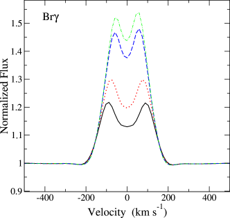
Figure 12: The dependency of Br$\gamma$ on the power-law index ($p$) of the local mass-loss rate per unit area, $\dot{m}$ (as in Section 5.1.2). The model line profiles are computed with $p=2.3$ (solid), $1.4$ (dot), $0.2$ (dash) and $0.0$ (dash-dot). The separation of the double peaks decreases as $p$ decreases. All other model parameters used here are same as in Model D (Table 6). The line profiles are computed at the inclination angle $i=70^{\circ}$.

References

- Alecian et al. (2013) Alecian E., et al., 2013, MNRAS, 429, 1001
- Bautista et al. (2004) Bautista M. A., Rudy R. J., Venturini C. C., 2004, ApJ, 604, L129
- Blandford & Payne (1982) Blandford R. D., Payne D. G., 1982, MNRAS, 199, 883
- Bouret & Catala (2000) Bouret J.-C., Catala C., 2000, A&A, 359, 1011
- Bouvier et al. (2003) Bouvier J., et al., 2003, A&A, 409, 169
- Bouvier et al. (2013) Bouvier J., Grankin K., Ellerbroek L. E., Bouy H., Barrado D., 2013, A&A, 557, A77
- Brittain et al. (2007) Brittain S. D., Simon T., Najita J. R., Rettig T. W., 2007, ApJ, 659, 685
- Burleigh et al. (2013) Burleigh K. J., Bieging J. H., Chromey A., Kulesa C., Peters W. L., 2013, ApJS, 209, 39
- Caratti o Garatti et al. (2013) Caratti o Garatti A., Garcia Lopez R., Weigelt G., Tambovtseva L. V., Grinin V. P., Wheelwright H., Ilee J. D., 2013, A&A, 554, A66
- Caratti o Garatti et al. (2015) Caratti o Garatti A., et al., 2015, A&A, 582, A44
- Castor (1970) Castor J. I., 1970, MNRAS, 149, 111
- Castor & Lamers (1979) Castor J. I., Lamers H. J. G. L. M., 1979, ApJS, 39, 481
- Cauley & Johns-Krull (2014) Cauley P. W., Johns-Krull C. M., 2014, ApJ, 797, 112
- Cauley & Johns-Krull (2015) Cauley P. W., Johns-Krull C. M., 2015, ApJ, 810, 5
- Chelli et al. (2009) Chelli A., Utrera O. H., Duvert G., 2009, A&A, 502, 705
- Cranmer (2008) Cranmer S. R., 2008, ApJ, 689, 316
- Cranmer (2009) Cranmer S. R., 2009, ApJ, 706, 824
- Decampli (1981) Decampli W. M., 1981, ApJ, 244, 124
- Donehew & Brittain (2011) Donehew B., Brittain S., 2011, AJ, 141, 46
- Drake et al. (2014) Drake J. J., Braithwaite J., Kashyap V., Günther H. M., Wright N. J., 2014, ApJ, 786, 136
- Dullemond et al. (2003) Dullemond C. P., van den Ancker M. E., Acke B., van Boekel R., 2003, ApJ, 594, L47
- Dzib et al. (2010) Dzib S., Loinard L., Mioduszewski A. J., Boden A. F., Rodríguez L. F., Torres R. M., 2010, ApJ, 718, 610
- Eaton & Herbst (1995) Eaton N. L., Herbst W., 1995, AJ, 110, 2369
- Edwards et al. (2006) Edwards S., Fischer W., Hillenbrand L., Kwan J., 2006, ApJ, 646, 319
- Eisner et al. (2014) Eisner J. A., Hillenbrand L. A., Stone J. M., 2014, MNRAS, 443, 1916
- Fairlamb et al. (2015) Fairlamb J. R., Oudmaijer R. D., Mendigutía I., Ilee J. D., van den Ancker M. E., 2015, MNRAS, 453, 976
- Garcia Lopez et al. (2006) Garcia Lopez R., Natta A., Testi L., Habart E., 2006, A&A, 459, 837
- Garcia Lopez et al. (2015) Garcia Lopez R., Tambovtseva L. V., Schertl D., Grinin V. P., Hofmann K.-H., Weigelt G., Caratti o Garatti A., 2015, A&A, 576, A84
- Ghosh & Lamb (1979) Ghosh P., Lamb F. K., 1979, ApJ, 232, 259
- Ghosh et al. (1977) Ghosh P., Pethick C. J., Lamb F. K., 1977, ApJ, 217, 578
- Grinin et al. (1991) Grinin V. P., Kiselev N. N., Chernova G. P., Minikulov N. K., Voshchinnikov N. V., 1991, Ap&SS, 186, 283
- Grinin et al. (1998) Grinin V. P., Rostopchina A. N., Shakhovskoi D. N., 1998, Astronomy Letters, 24, 802
- Harries (2000) Harries T. J., 2000, MNRAS, 315, 722
- Hartmann et al. (1994) Hartmann L., Hewett R., Calvet N., 1994, ApJ, 426, 669
- Herbst et al. (1987) Herbst W., et al., 1987, AJ, 94, 137
- Herbst et al. (1994) Herbst W., Herbst D. K., Grossman E. J., Weinstein D., 1994, AJ, 108, 1906
- Hubrig et al. (2009) Hubrig S., et al., 2009, A&A, 502, 283
- Hubrig et al. (2011) Hubrig S., et al., 2011, A&A, 536, A45
- Johansson & Letokhov (2004) Johansson S., Letokhov V. S., 2004, A&A, 428, 497
- Johns & Basri (1995) Johns C. M., Basri G., 1995, AJ, 109, 2800
- Knigge et al. (1995) Knigge C., Woods J. A., Drew E., 1995, MNRAS, 273, 225
- Königl (1991) Königl A., 1991, ApJ, 370, L39
- Kraus et al. (2008) Kraus S., et al., 2008, A&A, 489, 1157
- Kurosawa & Romanova (2013) Kurosawa R., Romanova M. M., 2013, MNRAS, 431, 2673
- Kurosawa et al. (2005) Kurosawa R., Harries T. J., Symington N. H., 2005, MNRAS, 358, 671
- Kurosawa et al. (2006) Kurosawa R., Harries T. J., Symington N. H., 2006, MNRAS, 370, 580
- Kurosawa et al. (2011) Kurosawa R., Romanova M. M., Harries T. J., 2011, MNRAS, 416, 2623
- Kurucz (1979) Kurucz R. L., 1979, ApJS, 40, 1
- Kwan et al. (2007) Kwan J., Edwards S., Fischer W., 2007, ApJ, 657, 897
- Lii et al. (2012) Lii P., Romanova M., Lovelace R., 2012, MNRAS, p. 2228
- Long & Knigge (2002) Long K. S., Knigge C., 2002, ApJ, 579, 725
- Matt & Pudritz (2005) Matt S., Pudritz R. E., 2005, ApJ, 632, L135
- Mendigutía et al. (2011) Mendigutía I., Eiroa C., Montesinos B., Mora A., Oudmaijer R. D., Merín B., Meeus G., 2011, A&A, 529, A34
- Montesinos et al. (2009) Montesinos B., Eiroa C., Mora A., Merín B., 2009, A&A, 495, 901
- Muzerolle et al. (2001) Muzerolle J., Calvet N., Hartmann L., 2001, ApJ, 550, 944
- Muzerolle et al. (2004) Muzerolle J., D’Alessio P., Calvet N., Hartmann L., 2004, ApJ, 617, 406
- Natta et al. (2000) Natta A., Grinin V. P., Tambovtseva L. V., 2000, ApJ, 542, 421
- Pasinetti Fracassini et al. (2001) Pasinetti Fracassini L. E., Pastori L., Covino S., Pozzi A., 2001, A&A, 367, 521
- Petrov et al. (2007) Petrov R. G., et al., 2007, A&A, 464, 1
- Petrov et al. (2014) Petrov P. P., Kurosawa R., Romanova M. M., Gameiro J. F., Fernandez M., Babina E. V., Artemenko S. A., 2014, MNRAS, 442, 3643
- Pontoppidan et al. (2007) Pontoppidan K. M., Dullemond C. P., Blake G. A., Boogert A. C. A., van Dishoeck E. F., Evans II N. J., Kessler-Silacci J., Lahuis F., 2007, ApJ, 656, 980
- Rodgers et al. (2002) Rodgers B., Wooden D. H., Grinin V., Shakhovsky D., Natta A., 2002, ApJ, 564, 405
- Romanova et al. (2003) Romanova M. M., Ustyugova G. V., Koldoba A. V., Wick J. V., Lovelace R. V. E., 2003, ApJ, 595, 1009
- Romanova et al. (2009) Romanova M. M., Ustyugova G. V., Koldoba A. V., Lovelace R. V. E., 2009, MNRAS, 399, 1802
- Romanova et al. (2013) Romanova M. M., Ustyugova G. V., Koldoba A. V., Lovelace R. V. E., 2013, MNRAS, 430, 699
- Rostopchina et al. (2001) Rostopchina A. N., Grinin V. P., Shakhovskoi D. N., 2001, Astronomy Reports, 45, 51
- Shu et al. (1994) Shu F., Najita J., Ostriker E., Wilkin F., Ruden S., Lizano S., 1994, ApJ, 429, 781
- Sobolev (1957) Sobolev V. V., 1957, Soviet Astron., 1, 678
- Strafella et al. (1998) Strafella F., Pezzuto S., Corciulo G. G., Bianchini A., Vittone A. A., 1998, ApJ, 505, 299
- Symington et al. (2005) Symington N. H., Harries T. J., Kurosawa R., 2005, MNRAS, 356, 1489
- Tambovtseva et al. (2014) Tambovtseva L. V., Grinin V. P., Weigelt G., 2014, A&A, 562, A104
- Tatulli et al. (2007) Tatulli E., et al., 2007, A&A, 464, 29
- Vieira et al. (2003) Vieira S. L. A., Corradi W. J. B., Alencar S. H. P., Mendes L. T. S., Torres C. A. O., Quast G. R., Guimarães M. M., da Silva L., 2003, AJ, 126, 2971
- Vollmann & Eversberg (2006) Vollmann K., Eversberg T., 2006, Astronomische Nachrichten, 327, 862
- Weigelt et al. (2007) Weigelt G., et al., 2007, A&A, 464, 87
- Weigelt et al. (2011) Weigelt G., et al., 2011, A&A, 527, A103
- de Winter et al. (1999) de Winter D., Grady C. A., van den Ancker M. E., Pérez M. R., Eiroa C., 1999, A&A, 343, 137