Accepted for publication in Journal of Memory and Language

Abstract

Generalized additive mixed models are introduced as an extension of the generalized linear mixed model which makes it possible to deal with temporal autocorrelational structure in experimental data. This autocorrelational structure is likely to be a consequence of learning, fatigue, or the ebb and flow of attention within an experiment (the `human factor'). Unlike molecules or plots of barley, subjects in psycholinguistic experiments are intelligent beings that depend for their survival on constant adaptation to their environment, including the environment of an experiment. Three data sets illustrate that the human factor may interact with predictors of interest, both factorial and metric. We also show that, especially within the framework of the generalized additive model, in the nonlinear world, fitting maximally complex models that take every possible contingency into account is ill-advised as a modeling strategy. Alternative modeling strategies are discussed for both confirmatory and exploratory data analysis.
 

Keywords: generalized additive mixed models, factor smooths, within-experiment adaptation, autocorrelation, experimental time series, confirmatory and exploratory data analysis, model selection
 
 

1 Introduction

Regression models are built on the assumption that the residual errors are identically and independently distributed. Mixed models make it possible to remove one source of non-independence in the errors by means of random-effect parameters. For instance, in an experiment with fast and slow subjects, the inclusion of by-participant random intercepts ensures that the fast subjects will not have residuals that will tend to be too large, and that the slow subjects will not have residuals that are too small (see, e.g. Pinheiro and Bates,, 2000, for detailed examples). However, even after including random-effect parameters in a linear model, errors can still show non-independence.

For studies on memory and language, it has been known for nearly half a century that in time series of experimental trials, response variables such as reaction times elicited at time $t$ may be correlated with earlier reaction times at $t-k,k\geq 1$ (Broadbent,, 1971; Welford,, 1980; Sanders,, 1998; Taylor and Lupker,, 2001; Gilden,, 2001; Gilden et al.,, 1995; Baayen and Milin,, 2010). One source of temporal dependencies between trials is the presence of an autocorrelational process in the errors, potentially representing fluctuations in attention. Another source may be habituation to the experiment, possibly in interaction with decisions made at preceding trials (Masson and Kliegl,, 2013). Alternatively, subjects may slow down in the course of an experiment due to fatigue. A further source of correlational structure in sequences of responses is learning. As shown by Marsolek, (2008), the association strengths between visual features and object names are subject to continuous updating. Ramscar et al., (2010) and Arnon and Ramscar, (2012) documented the consequences of within-experiment learning in the domain of language. Kleinschmidt and Jaeger, (2015) report and model continuous updating in auditory processing in the context of speaker-listener adaptation. De Vaan et al., (2007) reported lexical decisions at trial $t$ to be co-determined by the lexicality decision and the reaction time to a prime that occurred previously at $t-40$. Grammaticality judgements that change in the course of an experiment are reported by Dery and Pearson, (2015). We refer to the ensemble of learning, familiarization with the task, fatigue, and attentional fluctuations as adaptive processes, or, in short, the `human factor'. We also refer to data in which the human factor plays no role whatsoever as `sterile' data, data that are not infected in any way by hidden processes unfolding in time series of experimental trials.

Why might we expect that experimental data are not sterile? Because, unlike molecules or plots of barley, human beings adapt quickly and continuously to their environment, and as the work mentioned above has shown, this includes the environment of psycholinguistic experiments.

When temporal autocorrelations are actually present in the data, but not brought into the statistical model, the residuals of this model will be autocorrelated in experimental time. The proper evaluation of model components by means of $t$ or $F$ tests presupposes that residual errors are identically and independently distributed. By bringing random intercepts and random slopes into the model specification, clustering in the residuals by item or subject is avoided. However, such random slopes and random intercepts do not take care of potential trial-to-trial autocorrelative structure. The presence of autocorrelation in the residuals leads to imprecision in model evaluations and uncertainty about the validity of any significances reported. When strong autocorrelation characterizes the residuals, this uncertainty will make it impossible to draw well-founded conclusions about statistical significance.

It might be argued that adaptive processes, if present, will have effects that are so minute that they are effectively undetectable. If so, the experimental design, and only the experimental design, could serve as a guide for determining the statistical model to be fitted to the data. Alternatively, one might acknowledge the presence of adaptive processes but claim that their presence gives rise to random and temporally uncorrelated noise. Any such adaptive processes would therefore be expected not to interact with predictors of theoretical interest.

However, it is conceivable that adaptive processes are present in a way that is actually not harmless. We distinguish two cases. First, adaptive processes may be present, without interacting with critical predictors of theoretical interest. In this case, measures for dealing with the autocorrelation in the errors will be required, without however affecting the interpretation of the predictors. In this case, elimination of autocorrelation from the errors will result in p-values that are more trustworthy. Second, it is in principle possible that adaptive processes actually do interact with predictors of theoretical interest in non-trivial ways. If so, it is not only a potential autocorrelational process in the residual error that needs to be addressed, but also and specifically the adaptive processes. These processes, which themselves may constitute a considerable source of autocorrelation in the errors, will need to be examined carefully in order to provide a proper assessment of how they modulate the effects of the critical predictors.

In this study, we discuss three examples of non-sterile data demonstrably infected by adaptive processes unfolding in the experimental time series constituted by the successive experimental trials. First, we re-analyze a data set with multiple subjects, and a $2\times 2\times 4$ factorial design with true treatments (Kliegl et al.,, 2015) and a single stimulus `item'. We then consider a mega-study with auditory lexical decision (Ernestus and Cutler,, 2015) using a regression design with crossed random effects of subject and item. The third analysis concerns a self-paced reading study in which subjects were reading Dutch poems, following up on earlier analyses presented in Baayen and Milin, (2010).

The analyses of these three data sets make use of the generalized additive mixed model (gamm). Before presenting these analyses, we first provide an introduction to gamms. Section 4 discusses regression modeling strategies for dealing with the human factor when conducting confirmatory or exploratory data analysis, and the final discussion section, after summarizing the main results, closes with some reflections on the importance of parsimony in regression modeling.

2 The generalized additive mixed model

In linear regression, a univariate response $y_{i}$ (where $i$ indexes the individual data points) is modelled as the sum of a linear predictor $\eta_{i}$ and a random error term with zero mean. This linear predictor is assumed to depend on a set of predictor variables. Often, the response variable is assumed to have a normal distribution. If so, a regression model such as

$$y_{i}=\eta_{i}+\epsilon_{i}\text{ where }\epsilon_{i}\underset{\text{ind}}{\sim}N(0,\sigma^{2})\text{ and }\eta_{i}=\beta_{0}+\beta_{1}x_{1i}+\beta_{2}x_{2i}.$$

describes a response variable $y$ that is modeled as a weighted sum of two predictors, $x_{1}$ and $x_{2}$, together with an intercept ($\beta_{0}$) and Gaussian error with standard deviation $\sigma$.

Generalized linear models let the response depend on a smooth monotonic function of the linear predictor. This family of models allows the response to follow not only the normal distribution, but other distributions from the exponential family, such as Poisson, gamma, or binomial. An example of a binomial glm with the same linear predictor $\eta$ is

$$y_{i}\underset{\text{ind}}{\sim}\text{binom}(\exp(\eta_{i})/\{1+\exp(\eta_{i})\},1)\text{ where }\eta_{i}=\beta_{0}+\beta_{1}x_{1i}+\beta_{2}x_{2i}.$$

This equation specifies that $y_{i}$ follows a binomial distribution with `number of trials' = 1, and a probability of success $\exp(\eta_{i})/\{1+\exp(\eta_{i})\}$ that is dependent on the predictor variables. The generalized linear mixed model (glmm) enriches the glm with further sources of random noise, modeled with the help of Gaussian random variables with mean zero and unknown standard deviation to be estimated from the data. By way of example, if $y$ denotes response time, $x_{1}$ the amount of sleep deprivation, and $x_{2}$ temperature, an experiment carried out with multiple subjects $j$ would be analyzed with the model

$$y_{ij}=\eta_{ij}+\epsilon_{ij}\text{ where }\epsilon_{ij}\underset{\text{ind}}{\sim}N(0,\sigma^{2})\text{ and }\eta_{ij}=\beta_{0}+b_{j}+\beta_{1}x_{1i}+\beta_{2}x_{2i},\text{ with }b_{j}\underset{\text{ind}}{\sim}N(0,\sigma_{b}^{2}),$$

under the assumption that the only term in the model that has to be adjusted from subject to subject is the intercept. In other words, this model assumes that there are faster and slower subjects, and that in all other respects, subjects behave in the same way. Specifically, the effects of the predictors $x_{1}$ and $x_{2}$ are assumed not to vary across subjects. More complex models can be obtained by relaxing these assumptions (see, e.g., Pinheiro and Bates,, 2000). The $b_{j}$ given the estimate of $\sigma_{b}$ are known as best unbiased linear predictors (blups), conditional modes, or posterior modes.

A generalized additive mixed model (Hastie and Tibshirani,, 1990; Lin and Zhang,, 1999; Wood,, 2006, 2011; Wood et al.,, 2015) is a glmm in which part of the linear predictor $\eta$ is itself specified as a sum of smooth functions of one or more predictor variables. Thus, a generalized additive (mixed) model is additive in two ways. First, it inherits from the generalized linear model that the linear predictor is a weighted sum. The generalized additive model adds to this functions of one or more predictors that themselves are weighted sums of basis functions. An important property of gamms is that each term in the model specifies a partial effect, i.e., the effect of that specific term when all other terms in the model are held constant.

In what follows, we first discuss univariate splines, illustrated with the time series of reaction times of one subject (123) in the KKL dataset, a dataset we return to in more detail below. Following this, we introduce multivariate splines, using as example lexical decision latencies elicited for Vietnamese compound words.

2.1 Univariate splines

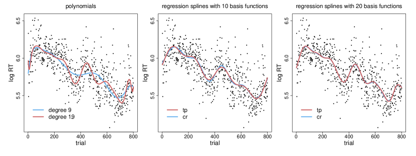
Figure 1: Log reaction time as a function of trial for subject 123 in the KKL data set. Left: fit with orthogonal polynomials of degree 9 and 19 (10 and 20 parameters including the intercept); Center: fit with regression splines with 10 basis functions; Right: fit with regression splines with 20 basis functions. cr: restricted cubic spline; tp: thin plate regression spline.

The left panel of Figure 1 presents the time series of subject 123 in the KKL data set, with trial number (1, 2, …, 800) on the horizontal axis, and log response time on the vertical axis. This plot reveals that as the experiment proceeded, this particular subject tended to respond more quickly. Although a linear model fitting a straight line to these data,

$$y_{i}=\beta_{0}+\beta_{1}x_{i}+\epsilon_{i},\text{ where }\epsilon_{i}\underset{\text{ind}}{\sim}N(0,\sigma^{2})$$

supports a downward trend ($p<0.0001$, aic = $-206.46$), it is clear that a straight line does not do justice to the undulating pattern that appears to ride on top of the linear trend. We therefore need to relax the linearity assumption, and allow the response $y$ to be a smooth function $f$ of $x$:

$$y_{i}=\beta_{0}+f(x_{i})+\epsilon_{i},\text{ where }\epsilon_{i}\underset{\text{ind}}{\sim}N(0,\sigma^{2}).$$

The regression smooth $f(x)$ is a weighted sum of a set of $q$ so-called basis functions defined over the predictor $x$ (Wood,, 2006; James et al.,, 2013). Writing $B_{k}$ for the $k$-th basis function, we have that

$$f(x_{i})=\sum_{k=1}^{q}B_{k}(x_{i})\beta_{k}.$$ (1)

The question is how to choose these basis functions. One might consider using polynomials of $x$, i.e, basis functions of the form

$$B_{k}(x_{i})=x_{i}^{k},\hskip 10.00002ptk=0,1,\ldots,$$

which leads to regression models with a polynomial of degree $d$ and $d+1$ parameters:

$$y_{i}=\beta_{0}x_{i}^{0}+\beta_{1}x_{i}^{1}+\beta_{2}x_{i}^{2}+\beta_{3}x_{i}^{3}+\ldots+\beta_{d}x_{i}^{d}+\epsilon_{i},\text{ where }\epsilon_{i}\underset{\text{ind}}{\sim}N(0,\sigma^{2}).$$

The blue curve in the left panel of Figure 1 presents the fit of a polynomial of degree $d=9$, which requires 10 $\beta$ coefficients (one for the intercept, and 9 for the non-zero powers of $x$). Although this model provides an improved fit to the data (aic = $-274.74$), visual inspection suggests it oversmoothes the data. A polynomial of degree $d=19$, shown in red, follows the trend in the data more closely, and provides a substantially improved fit (aic = $-332.27$). Unfortunately, the undulations for the earliest and latest trials look artefactual, and suggest undersmoothing. More in general, higher-order polynomials come with several undesirable properties when interest is in the behavior of the response variable over the full range of the predictor. The present artefactual wiggliness at the edges of the predictor domain, where data are sparse, illustrates one such undesirable property. Regression splines have been developed to avoid such artefacts.

There are many different kinds of splines, we restrict ourselves here to two particular splines: restricted cubic splines (cr) and thin plate regression splines (tp). The center and right panels of Figure 2 illustrates these splines for 10 and 20 basis functions respectively. The blue curves represent restricted cubic splines, and the red curves, thin plate regression splines. With 10 basis functions (and 10 parameters), the splines already capture the trend in the data much better than the corresponding 10-parameter polynomial (aic cr = $-316.75$, aic tp = $-311.4$), for 20 basis functions, fits are comparable to that of the polynomial of degree 20 (aic cr = $-331.52$, aic tp = $-334.06$) but without edge artifacts.

Figure 2: Log reaction time as a function of trial (scaled to the [0,1] interval) for subject 123 in the KKL data set, with an unpenalized restricted cubic spline and its basis functions. Vertical black lines indicate knots. The numbers above these lines are the (unpenalized) weights for the basis functions. Note that for any given basis function, the maximum is reached at exactly one knot, whereas at all other knots, it is zero.

The basis functions for the cr regression spline in the center panel of Figure 1 are illustrated in Figure 2. Again, the horizontal axis represents trial number, and the vertical axis log response time. The data points are shown, together with the restricted cubic spline smooth (in red). The basis functions all have the same functional form, the mathematical definition of which can be found in, e.g., Wood (2006, chapter 4). Each basis function is a curve that itself is made up of sections of cubic polynomials, under the constraint that the function must be continuous up to and including the second derivative. The points at which the sections of the curve meet are referred to as knots. In Figure 1, these knots are indicated by vertical black lines. The numbers above these black lines represent the weights $\beta_{k}$ (cf. equation 1) for the basis functions that have their maximum above these knots. In this parameterization of restricted cubic regression splines, any given basis function has its maximum at one specific knot, and is zero at all other knots.

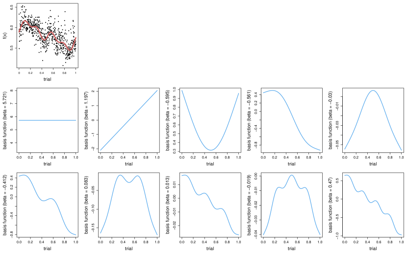
Figure 3: Log reaction time as a function of trial (scaled to the [0,1] interval) for subject 123 in the KKL data set, with an unpenalized thin plate regression spline (upper left) and its basis functions. The Y-axes for the basis functions have different scales, as the basis functions have been weighted (unpenalized weights in parentheses). Note, first, that the first two basis functions are not wiggly but completely smooth, and that the amount of wiggliness of the remaining thin plate basis functions increases from left to right and top to bottom.

The basis functions for a thin plate regression spline are constructed in a different way. Figure 3 illustrates the 10 basis functions for the tp smooth in the second panel of Figure 1. The first basis function is a horizontal line, allowing calibration of the intercept. The second basis function is a straight line, allowing the model to capture linear trends. Note that the slope of this line can be reversed by using a negative weight.

Whereas the first two basis functions are completely smooth, the remaining basis functions are wiggly. The exact form of these basis functions depends on the number of basis functions requested, as well as on whether the basis function is the first, second, third, …, of the requested wiggly basis functions (for mathematical details, see, e.g., Wood 2006, chapter 4). What is important is that each successive basis function is more wiggly than the preceding one. Thus, each additional basis function makes it possible to model more subtle aspects of the wiggliness in the data. Here too, negative weights will reverse the orientation of the basis functions, changing for instance a parabola that opens upward in a parabola that opens downward.

Figure 4: Edf per basis function for a thin plate regression spline with penalty order $m=2$ fitted to the time series of reaction times of subject 123 in the KKL data set. The first two basis functions (in red) are completely smooth functions (a horizontal straight line and a tilted straight line), which cannot be penalized for wiggliness.

At this point, we are faced with the question of what the optimal number of basis functions is. On one hand, we want to be faithful to the data, but on the other hand, we also want to avoid overfitting and incorporating spurious wiggliness, such as observed for the polynomial of degree 20 in the left panel of Figure 1. The solution offered by spline theory is to start with $k$ basis functions, and to select that vector of estimated coefficients $\hat{\bm{\beta}}$ such that the quantity Q,

$$Q=\sum_{i}(y_{i}-f(x_{i}))^{2}+\lambda\int f^{\prime\prime}(x)^{2}dx,$$ (2)

is minimized. $Q$ will be smaller when the weights are chosen such that the summed squared error is smaller. At the same time, $Q$ will be larger for smooths with greater wiggliness, quantified by the integral over the squared second derivative of the smooth. The balance of the constraint to stay faithful to the data and to avoid excess wiggliness is regulated by the smoothing parameter $\lambda$. When $\lambda=0$, all that counts is faithfulness to the data, irrespective of how complex the spline smooth is. As $\lambda$ is increased, the complexity of the spline comes into play, and undersmoothing becomes more and more costly.

The appropriate amount of penalization (given by an optimal $\lambda$) can be estimated by prediction error methods (cross-validation) or by marginal likelihood. The latter method (used in the present study) requires a prior on the distribution of the coefficients $\bm{\beta}$. This prior expresses mathematically that the `truth' is more likely to be smooth than wiggly (cf. Occam's razor). The smoothing parameter $\lambda$ gets tuned in order that random draws from the prior on the $\bm{\beta}$ coefficients that is implied by $\lambda$ have high average likelihood. This Bayesian approach is also used for variance estimation, making for easier confidence interval calculation while at the same time providing good coverage probabilities (Nychka,, 1988; Marra and Wood,, 2012).

Given $k$ basis functions, penalization will typically result in a model with effective degrees of freedom less than $k$: $k$ specifies the maximum possible degrees of freedom for a model term. However, it is possible that the initial dimensionality selected is too low. Doubling the number of basis functions and re-fitting will show whether this is indeed the case. Checking that $k$ is not too restrictive is an essential part of working with gams.

An important consequence of penalization is that the coefficients $\bm{\beta}$ are no longer free to vary. The values of these coefficients will be smaller than if there were no penalization (i.e., if $\lambda$ were zero). The extent to which a coefficient is smaller under penalization, its shrinkage factor, is bounded between 0 and 1 and is referred to as its effective degrees of freedom (edf). Figure 4 illustrates the effective degrees of freedom for a thin plate regression spline with 60 basis functions, fitted to the time series of reaction times of subject 123 in the KKL dataset. The first two basis functions (in red) are straight lines and hence receive no penalty for wiggliness. The remaining basis functions are wiggly. Most of the second half of the basis function (index $>30$) are severely penalized.

When a thin plate regression spline is fitted to data with a linear trend, the wiggly basis functions will be strongly penalized whereas the two linear basis functions are retained without penalization. Setting aside the edf of 1 for the intercept, the edfs for such a smooth will be 1 or slightly greater than 1, as the slope of the second basis function requires 1 parameter. If the data follow a quadratic trend, the edf will be close to 3, with a strong weight for the third basis function. However, edfs for thin plate regression splines close to 3 may also be indicative of other trends, such as downward trends that level off for larger values of the predictor.

The sum of the edf's of the basis function is used for significance testing in model comparison. For instance, a comparison of the abovementioned models using thin plate regression splines with 10 and 20 basis functions shows that increasing the number of basis functions results in a decrease of the residual deviance of 1.1664 at the cost of 15.4248 (the total edf of the more complex model) $-$ 9.6448 (the total edf of the simpler model) $=$ 5.78 edfs. An F-test ($F=6.01,p<0.0001$) suggests that the investment in a more complex model pays off.

Thus far, we have considered the time series of only one subject. When multiple subjects are considered simultaneously, we need a generalized additive mixed model (gamm). As a first step, we may consider a model with by-subject random intercepts $b_{j}$:

$$y_{ij}=\beta_{0}+f(x_{i})+b_{j}+\epsilon_{ij}\text{ where }\epsilon_{ij}\underset{\text{ind}}{\sim}N(0,\sigma^{2})\text{ and }b_{j}\underset{\text{ind}}{\sim}N(0,\sigma_{b}^{2}).$$

Random effects are implemented as parametric terms penalized by a ridge penalty (James et al.,, 2013), which is equivalent to the assumption that the coefficients are independently and identically distributed normal random effects. The implementation of random effects by means of ridge penalties does not exploit the sparse structure of many random effects, and hence they are more costly to compute than corresponding random effects in the linear mixed model.

The above model is unsatisfactory, however, because it assumes that each subject goes through the experiment in exactly the same way. At the very least, we need to allow for separate regression splines $f_{j}(x)$ for different subjects $j$:

$$y_{ij}=\beta_{0}+f_{j}(x_{i})+b_{j}+\epsilon_{ij}\text{ where }\epsilon_{ij}\underset{\text{ind}}{\sim}N(0,\sigma^{2})\text{ and }b_{j}\underset{\text{ind}}{\sim}N(0,\sigma_{b}^{2}).$$

This model incorporates a nonlinear interaction of subject by trial, but restricts by-subject random effects to the intercept. Since each individual subject's regression smooth $f_{j}(x)$ comes with its own penalization parameter $\lambda_{j}$, subjects' time series of reaction times are effectively treated as fixed, just as the slopes of by-subject regression lines in the following linear mixed model are fixed:

$$y_{ij}=\beta_{0}+b_{j}+\beta_{j}x_{i}+\epsilon_{ij}\text{ where }\epsilon_{ij}\underset{\text{ind}}{\sim}N(0,\sigma^{2})\text{ and }b_{j}\underset{\text{ind}}{\sim}N(0,\sigma_{b}^{2}).$$

A linear mixed model with random intercepts and random slopes,

$$y_{ij}=\beta_{0}+\beta_{1}x_{i}+b_{0j}+b_{1j}+\epsilon_{ij}\text{ where }\epsilon_{ij}\underset{\text{ind}}{\sim}N(0,\sigma^{2})\text{ and }\bm{b}_{j}=\left[\begin{array}[]{c}b_{0j}\\ b_{1j}\end{array}\right]\sim N(\bm{0},\bm{\Psi}),$$

$$\text{ with }\bm{\Psi}=\left[\begin{array}[]{cc}\sigma_{0}&\rho\sigma_{0}\sigma_{1}\\ \rho\sigma_{0}\sigma_{1}&\sigma_{1}\end{array}\right],$$

has as non-linear equivalent a gamm with a factor smooth interaction (henceforth abbreviated to factor smooth). A factor smooth implements two measures to ensure that effects are proper random effects. First, a single smoothing parameter $\lambda$ is used for each of the subject-specific smooths for trial, forcing penalization to shrink the parameters of the basis functions in the same way for all subjects. Second, penalization is allowed to affect the second (completely smooth) basis function that under standard penalization for wiggliness would not have been effected. This is achieved through additional penalization of the penalty null space. In the situation that there is true wiggliness, a factor smooth will capture this. When there is no wiggliness, a factor smooth will return random intercepts.

The edf values listed in the tables in the appendix for F-tests on the smooths are based on the sum of the edfs of their basis functions, from which the edf for the intercept (equal to 1) has been subtracted, as the intercept is evaluated separately as a parametric term in the model. The p-values listed in these tables for the smooth terms are based on specific $F$ ratios that are discussed in detail in Wood, 2013a for regression splines and in Wood, 2013b for random effects. The tests for the regression splines are conditional on the estimates for the smoothing parameters for other splines in the model. The test for random effects treats the variance components that are not tested as fixed at their estimates. This assumption makes it possible to test for a zero effect in a computationally efficient way. Wood, 2013b points out that this test is likely to be less reliable under three circumstances: when variance parameters are not well estimated, when the assumption that the posterior modes follow a normal distribution is violated, and when covariates in small samples are highly correlated. Especially for logistic models with small sample sizes and correlated covariates, caution is required when p-values are around the threshold for accepting or rejecting a random effect as significant.

2.2 Multivariate splines

Thus far, we have considered univariate smooths $f(x)$, but multivariate regression splines $f(x_{1},x_{2},\ldots)$ are also available. By way of example, we consider lexical decision latencies for 15,021 Vietnamese compound words in a single-subject experiment reported in Pham and Baayen, (2015). (The data for the analyses reported here and in subsequent sections are, unless specified otherwise, available in the RePsychLing package for R at https://github.com/dmbates/RePsychLing.)

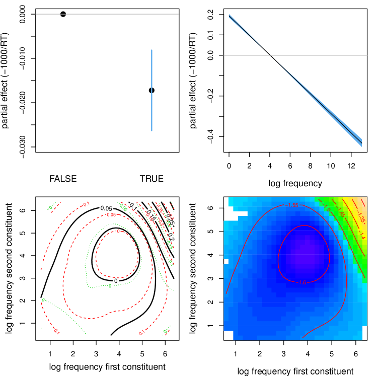
Figure 5: A simplified model for Vietnamese lexical decision latencies to compound nouns, with an effect of tone (upper left), word frequency (upper right), and the left and right constituent frequencies (bottom panels). The lower left panel shows contour lines with 1SE confidence intervals, the lower right panel presents the corresponding contour plot. Lighter and warmer colors denote longer response latencies.

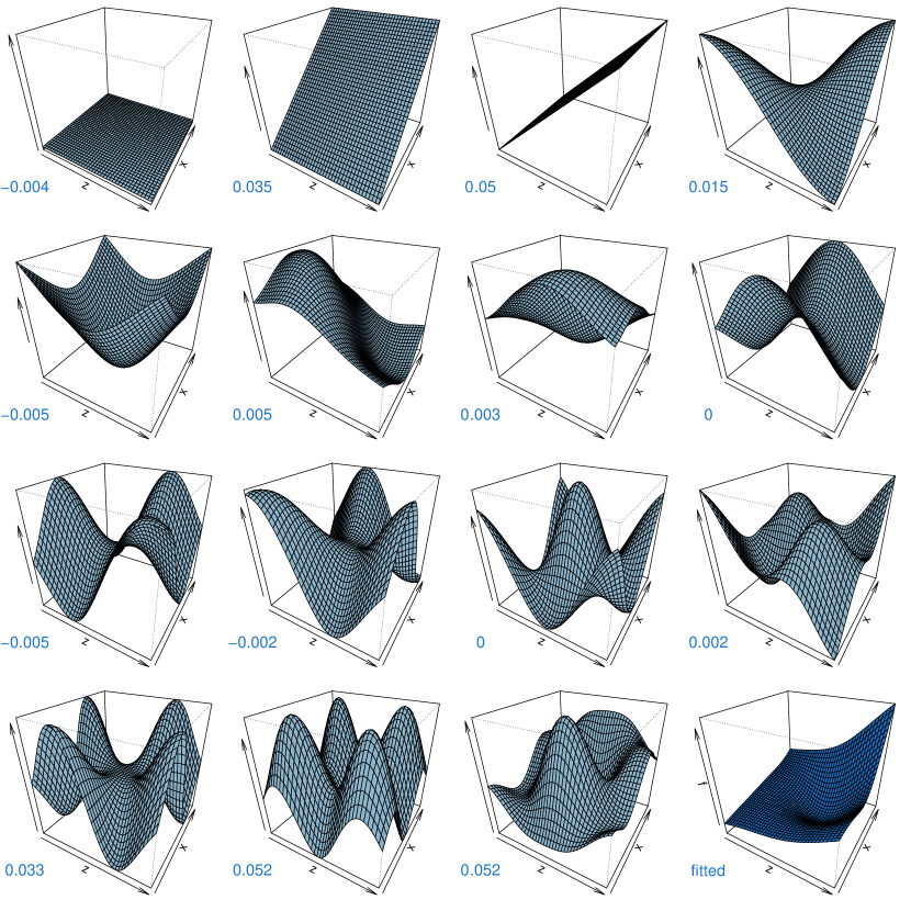
Figure 6: Basis functions and their weights for a thin plate regression spline for the interaction of the constituent frequencies in the gam fitted to the Vietnamese lexical decision data.

Figure 5 presents a (simplified) model for these visual lexical decision latencies with four predictors. First, we include a factor specifying whether the tone realized on the first constituent of a Vietnamese compound is the most common (mid-level) tone, or another of six tones. We use the notation $t(i)$ to denote the level of $\alpha$ for observation $i$, with as possible values true and false. The effect of tone ($\alpha_{t(i)}$) is coded with treatment coding. Second, we included the frequency of the compound word ($x_{1}$). Additional predictors were the frequencies of the first and second constituents ($x_{2}$ and $x_{3}$). We used a univariate thin plate regression spline for compound frequency, and we used a tensor product smooth for the interaction of the two constituent frequencies:

$$y_{i}=\beta+\alpha_{t(i)}+f_{1}(x_{1i})+f_{2}(x_{2i},x_{3i})+\epsilon_{i},\text{ where }\epsilon_{i}\underset{\text{ind}}{\sim}N(0,\sigma^{2}).$$

Before discussing the details of bivariate splines, first consider Figure 5, which presents the partial effects of the predictors, i.e., the contributions of the individual terms in the model. The upper left panel visualizes the effect of tone. The reference level (some other tone than the mid tone) is at zero. Words with a mid tone on the first constituent are responded to -0.0172 units faster on the -1000/RT scale. The group means for tone (with the other predictors held at their most typical values) are obtained by adding the intercept, resulting in the estimates $-1.601$ and $-1.601-0.017=-1.618$.

Frequency was entered into the model with a thin plate regression spline, but its effect is linear, and it is this linear effect that is returned by the regression spline. The confidence intervals for the line have width zero where they intersect with the horizontal line crossing 0 on the y-axis. This is because for a gam to be identifiable, all uncertainty about the intercept is already quantified through the standard deviation for the intercept. Since the upper right panel shows the partial effect of word frequency, the regression line has to be shifted by the value of the intercept ($-1.601$) to position it at its appropriate vertical position familiar from standard graphs of regression lines. After this shift, the word frequency $f_{0}$ for which the regression line crosses the horizontal axis now has the intercept as new $y$ value. But as all uncertainty about the intercept is bundled into the standard deviation estimated for the intercept, there is no uncertainty left about the contribution of $f_{0}$ to the model's prediction. As a consequence, the confidence interval for the partial effect of frequency is zero at $f_{0}$.

The bottom panels of Figure 5 visualize the interaction of the two constituent frequencies. Shortest responses are found for intermediate values, the longest response times occur when both frequencies are high. The lower left panel shows contour lines with 1SE confidence intervals, red dashed lines represent the lower interval, and green dotted lines the higher interval. The contour plot in the lower right facilitates interpretation with color coding. Deeper shades of blue indicate shorter reaction times.

This interaction can be modeled with the help of a bivariate thin plate regression spline or with a tensor product smooth. A thin plate regression smooth $y=f(x,z)$ models a wiggly surface as a weighted sum of simpler surfaces, as illustrated in Figure 6. There are three completely smooth surfaces, a horizontal flat plane and two tilted planes. The remaining surfaces (from left to right and top to bottom) are increasingly wiggly. The weighted sum of these surfaces results in the surface in the lower right, the predicted surface for the interaction of the two constituent frequencies ($x$: first constituent, $z$: second constituent). Just as for univariate thin plate regression splines, penalization ensures a proper balance between oversmoothing and undersmoothing.

Multivariate thin plate regression splines are appropriate for isometric predictors, i.e., predictors that are measured on the same scale, such as longitude and latitude, or first and second constituent frequency. When predictors are on different scales, thin plate regression splines cannot be used. For interactions of non-isometric predictors, tensor product smooths are available. A bivariate tensor smooth makes use of basis functions that are the three-dimensional counterpart of the two-dimensional basis functions shown in Figure 2 for the univariate case. These basis functions are illustrated in the left-hand side of Figure 7. When 8 basis functions are selected for both predictor dimensions, a total of $8\times 8=64$ basis functions is set up. Each basis function is weighted, resulting in predicted values $y$ represented in Figure 7 by $64$ black dots, each representing the maximum of the basis function for the corresponding knot. Penalization requires two smoothing parameters, one for each dimension, and is implemented such that the black curves parallel to the X-axis, and those parallel to the Z-axis, are properly constrained (see Wood, 2006, chapter 4, for further details). Tensor product smooths applied to isometric predictors tend to produce similar results as thin plate regression splines, but for isometric predictors, thin plate regression splines tend to offer more precision. For the Vietnamese compounds, the two smooths predict regression surfaces that are nearly indistinguishable.

Figure 7: Examples of the basis functions used in bivariate tensor product smooths are illustrated to the left. The right illustrates the predicted wiggly surface for the partial effect of the constituent frequencies in the gam fitted to the Vietnamese reaction times. Each dot represents the top of a weighted basis function.

2.3 Interactions with factorial predictors

It is often the case that a covariate has a functional form that differs for the individual levels of a factor. Different wiggly curves or wiggly (hyper)surfaces can be fitted to each factor level, as in the model

$$y_{i}=\beta+\alpha_{t(i)}+f_{1}(x_{1i},\text{by}=t(i))+f_{2}(x_{2i},x_{3i},\text{by}=t(i))+\epsilon_{i},\text{ where }\epsilon_{i}\underset{\text{ind}}{\sim}N(0,\sigma^{2}),$$

where $f_{i}(x_{1},x_{2},\ldots,\text{by}=t(i))$ denotes the smooth for the interaction of $x_{1},x_{2},\ldots$ by $\alpha$. For models with these kind of interactions, the main effect of the factor ($\alpha_{t(i)}$) is an important component of the model, as it has the crucial function of properly calibrating the different curves, surfaces (or hypersurfaces) with respect to the intercept. Gams can also be set up to estimate the difference between curves or (hyper)surfaces.

The analyses in this study were carried out with the help of the mgcv package, version 1.8-12 (Wood,, 2006, 2011) and the itsadug package (van Rij et al.,, 2016) for R (version 3.2.2, R Core Team,, 2015). These analyses are all exploratory, in that a sequence of increasingly complex models was constructed and only those predictors and interactions were maintained that received substantial support for improving the model fit.

This completes the introduction to the generalized additive (mixed) model. We now return to the central topic of this study, and turn to the first dataset illustrating that experimental data can be infected by the human factor in a non-trivial way.

3 The human factor in three experiments

3.1 The KKL dataset

The experiment reported by Kliegl et al., (2015), a follow up to Kliegl et al., (2011), showed that validly cued targets on a monitor are detected faster than invalidly cued ones, i.e., spatial cueing effect (Posner,, 1980) and that targets presented at the opposite end of a rectangle at which the cue had occurred were detected faster than targets presented at a different rectangle but with the same physical distance, an object-based effect (Egly et al.,, 1994). The sequence of an experimental trial is shown in Figure 8. Different from earlier research, the two rectangles were not only presented in cardinal orientation (i.e., in horizontal or vertical orientation), but also diagonally (45 degrees left or 45 degrees right). This manipulation afforded a follow up of a hypothesis that attention can be shifted faster diagonally across the screen than vertically or horizontally across the screen (Kliegl et al.,, 2011; Zhou et al.,, 2006). Finally, data are from two groups of subjects, one group had to detect small targets and the other large targets. For an interpretation of fixed effects relating to the speed of visual attention shifts under these experimental conditions we refer to Kliegl et al., (2015).

Figure 8: Sequence of events in visual-spatial attention experiment with an invalid cue on the same object. Screen 2: Left end of top rectangle is cued. Screen 3: SOA of 200 ms, Screen 4: Large target to be detected at right end of top rectangle (from Kliegl et al., 2011). In the new experiment rectangles were also presented in diagonal orientations; a different group of subjects was tested with small targets.

Eighty-six subjects participated in this experiment. There were 800 trials requiring detection of a small or large rectangle and 40 catch trials. The experiment is based on a size (2) $\times$ cue-target relation (4) $\times$ orientation (2) design. Targets were small or large; rectangles were displayed either in cardinal or diagonal orientation, and cue-target relation was valid (70% of all trials) or invalid in three different ways (10% of trials in each of the invalid conditions), corresponding to targets presented (a) on the same rectangle as the cue, but at the other end, (b) at the same physical distance as in (a), but on the other rectangle, or (c) at the other end of the other rectangle. Size of target was varied between subjects, the other two factors within subjects. The three contrasts for cue-target relation test differences in means between neighboring levels: spatial effect, object effect, and gravitation effect (Kliegl et al.,, 2011). Orientation and size factors are also included as numeric contrasts in such a way that the fixed effects estimate the difference between factor levels. With this specification the intercept estimates the grand mean of the 16 ($=2\times 4\times 2$) experimental conditions. The data are available as KKL in the RePsychLing package. The dependent variable is the log of reaction time for correct trials completed within a 750 ms deadline. The total number of responses was 53765.

Bates et al., (2015) determined a parsimonious mixed model for these data, dealing with issues of overparameterization. We refitted this model using in addition a quadratic polynomial, which allowed us to include a well-supported nonlinear effect for stimulus onset asynchrony, which was varied randomly in an interval ranging from 300 to 500 ms in this experiment, but the effect of which had not been included in the initial lmm report of Bates et al. (2015).

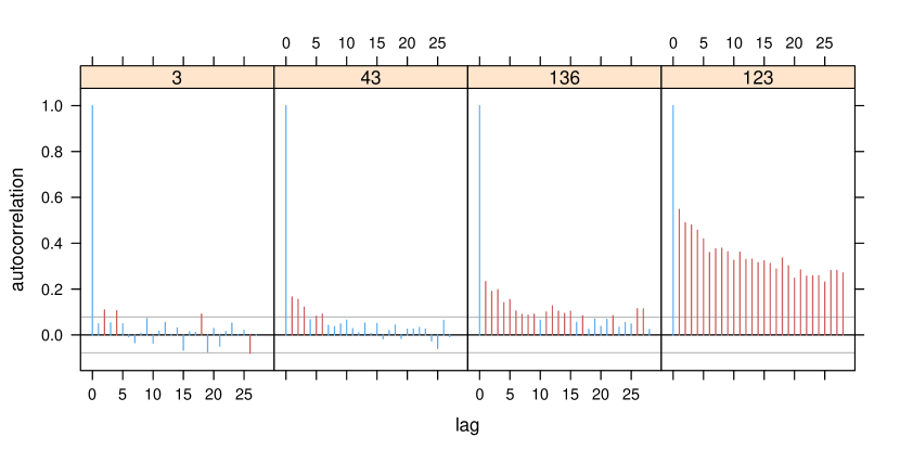
Figure 9: Autocorrelation functions for the residuals of a linear mixed model for four subjects in the KKL dataset (upper panels), and the corresponding plots (lower panels) graphing log reaction time (RT) against trial, with a loess smoother (span = 0.2, in blue) and a gam factor smooth (red).

Model criticism is an important but all too often neglected part of data analysis. Inspection of the residuals of the reference model reveals that although the residuals approximately follow a normal distribution, and although they are identically distributed, they are not independent.

The reaction times of a given subject constitute a time series, with experimental trial as unit of time. These trials can be ordered from the initial trial in the experimental list of trials, to the final trial in that list. In what follows, we refer to the time series of trials with the covariate Trial $=1,2,\ldots,k$. For the present experiment, we have 86 such time series, one for each of the 86 subjects. When we consider the residuals of the reference model, ordered by these time-series, we observe autocorrelative structure.

The strength of the autocorrelations in these by-subject time series varied from subject to subject. For four exemplary subjects in the top panels of Figure 9, the autocorrelation function is shown for the residuals of a linear mixed model fitted to the KKL dataset. The autocorrelations for the subject in the top left panel are quite mild, and unlikely to adversely affect model statistics. For the second subject, we find evidence for autocorrelations up to at least lag 3. Autocorrelations increase for the third subject, and are still present at a lag of 15 trials. The subject in the rightmost panel show strong autocorrelations, indicating that a response time at trial $t$ is remarkably well correlated with the response at time $t-L$, for lags $L$ as large as 25.

Given that the residuals of the reference model (refitted with a gamm) are not independent, it is unclear how reliable the estimates of model parameters and the assessments of the uncertainty about these estimates actually are. For this particular data set, strong autocorrelations such as for the last subject are exceptional, and hence it is likely that conclusions based on this model will be somewhat accurate. Nevertheless, a statistical model that is formally deficient is unsatisfactory, especially as there must be hidden temporal processes unfolding in this experiment that are not transparent to the analyst. Since the KKL data are clearly not sterile, a more fertile approach is to bring such hidden processes out in the open, and incorporate them into the statistical model.

Why are these autocorrelations present? In order to address this question, consider the plots in the lower set of panels of Figure 9. These panels present scatterplots of the data points for the four subjects in the corresponding top panels, to which two smoothers have been added, a loess locally weighted scatterplot smoother (Cleveland,, 1979) in blue and a smoother obtained with a generalized additive model in red. For subject 3, whose time series of responses hardly shows any autocorrelation, we observe smooths that are close to horizontal lines. As the experiment proceeds, there are only very small changes in average response time. When we move further to the right in the array of panels, temporal patterns begin to emerge. As the experiment proceeded, subjects responded more quickly. Furthermore, it appears that there may be undulations in response speed. These oscillating changes in amplitude, if real, may reflect slow changes in subjects' attention or concentration over the course of the experiment. By contrast, the general downward trend present for subjects 43, 136, and especially 123 may point to familiarization with and gradual optimization of response behavior for the task.

Figure 10: Loess smooths (span = 0.2) for the three-way interaction of Trial by Orientation by Size.

The presence of a potential learning effect raises the question of whether learning proceeded in the same way across the different experimental conditions. Graphical exploration suggests that the rate at which subjects respond faster over time indeed varies, specifically so across the levels of size and orientation, as shown in Figure 10. In the upper panels (diagonal orientation), reaction times decrease over the first half of the experiment and then level off, with a somewhat greater increase for small size. For cardinal orientation, reaction times decrease more quickly early on in the experiment, level off near the middle of the experiment, and then continue their descent for the condition with size big.

Within the context of the linear mixed model, the observed effects of trial can be taken into account by incorporating by-subject random slopes for Trial, and by allowing Trial to interact with Size and Orientation. As shown in Table 1, these extensions of our reference model are solidly supported by model comparisons using likelihood ratio tests. A summary of the final linear mixed model can be found in Table 3 in the appendix.

	Df	AIC	logLik	deviance	Chisq	Df	Pr($>$Chisq)
reference model	25	-25087.68	12568.84	-25137.68
add Trial L * (sze+orn)	28	-25884.64	12970.32	-25940.64	802.96	3	$<0.0001$
add Trial Q * (sze+orn)	31	-26174.41	13118.20	-26236.41	295.77	3	$<0.0001$
add random slopes Trial	33	-26988.91	13527.45	-27054.91	818.50	2	$<0.0001$

Table 1: Model comparisons for linear mixed models fitted to the KKL dataset. L: linear term of a quadratic polynomial; Q: quadratic term of this polynomial; sze: Size; orn: Orientation.

Figure 11 presents the autocorrelation functions for the residuals of this final, comprehensive, linear mixed model. Comparison with the top panels of Figure 9 shows that for subjects 136 and 123, the autocorrelation in the residuals has been reduced substantially, thanks to bringing the effects of Trial into the model. Nevertheless, some autocorrelation remains present.

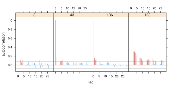
Figure 11: Autocorrelations in the residuals of the extended linear mixed model fitted to the KKL data.

For further reduction of autocorrelations, it is necessary to relax the assumption that the subject-specific effects of Trial, currently modeled by means of by-subject random intercepts and random slopes, are strictly linear. The smooths presented in the bottom panels of Figure 9 suggest that undulations may ride on top of the linear trends. What we need, then, is a way of relaxing the linearity assumption for the by-subject random effects of Trial. The factor smooth interaction of the generalized additive mixed model provides the required nonlinear counterpart to the combination of random slopes and random intercepts. A factor smooth for Trial by subject sets up a separate smooth for each level of the factor Subject. When we add the constraint that each smooth should have the same smoothing parameter, and penalize the smooths for wiggliness, thereby shrinking them towards zero, we obtain `wiggly random effects'.

The red smooths in Figure 9 are such factor smooths. They are very similar to the loess smooths, but are slightly more sensitive to the undulations in the data. Althought it might seem there is a risk that the factor smooths are modeling noise rather than signal, this is unlikely as the factor smooths are evaluated within the general framework of the generalized additive mixed model, and hence it is possible to assess whether they contribute significantly to the model fit. By way of example, across 100 random permutations of Trial for the four subjects of Figure 9, a significant factor smooth was obtained in 3 instances for $\alpha=0.05$ and for zero cases for $\alpha=0.01$, indicative of nominal Type I error rates. This example illustrates informally that factor smooths are unlikely to find and impose nonlinear structure when there is none.

Importantly, we think the undulating random effects captured by factor smooths represent the ebb and flow of attention. They emerge not only in the present data set, but have been observed for visual lexical decision (Mulder et al.,, 2014) as well as for word naming and for eeg data (Baayen et al., 2016b, ). If this interpretation is correct, penalized factor smooths are the appropriate statistical tool to use. We explicitly do not want to model these fluctuations in attention as fixed effects, because there is no reason to believe that if the experiment were replicated, a given subject would show exactly the same pattern. It is more realistic to expect that changes in attention will again be present, with roughly the same magnitude, but with ups and downs occurring at different points in time. In other words, we are dealing here with temporally structured noise, and the penalized factor smooths make it possible to bring such `wiggly random effects' into the statistical model.

	aic	freml	Df	comparison with	Chisq	Df difference	$\Pr(>\text{Chisq})$
reference model	-26009.55	-12495.77	27
linear model	-28047.29	-13422.25	34	reference model	926.5	7	$<$ 0.0001
factor smooths	-30876.72	-14500.08	31	linear model	1077.8	-3	$\dagger$
smooth trial	-31040.29	-14582.64	33	factor smooths	82.6	2	$<$ 0.0001

Table 2: Model comparison for gamms fitted to the KKL dataset. (The reference and linear models were refitted with gamms to ensure comparability across all four models.) $\dagger$: the model with factor smooths has lower freml (fast REML, see mgcv documentation) and fewer parameters, and thus is simpler and better, than the linear model.

Table 2 lists four gamms that we fitted to the KKL data. The first is the reference model, but refitted with gam software (the mgcv package for R), rather than with lmm software (the lme4 package for R), with as the only change that a thin plate regression spline is used for the SOA covariate, instead of a quadratic polynomial. The second model has the same specification as the final linear mixed model (summarized in Table 3 in the appendix), but refitted with a gamm. (These two models were refitted because both the estimation algorithms and the way in which degrees of freedom are handled differ between lme4 and mgcv.) As expected, the linear model, which includes effects for Trial, outperforms the reference model. The third model, which replaces the by-subject random intercepts and slopes by factor smooths, provides a better fit with fewer effective degrees of freedom. Addition of the three-way interaction of Trial by Size and Orientation improves the model further.

Figure 12: The Trial by Orientation by Size interaction in the full gamm model for the KKL data.

Figure 12 visualizes this three-way interaction of Trial by Orientation by Size estimated by the gamm (cf. Figure 10 for the corresponding loess smooths). The effect of learning is larger for the cardinal presentation (upper panels) than for the diagonal presentation (bottom panels). For both large (left panels) and small (right panels) stimuli, we observe rapid initial learning, which levels off more for small than for large stimuli. Big stimuli with diagonal presentation elicited the most smooth accommodation pattern, with response times gradually becoming shorter.

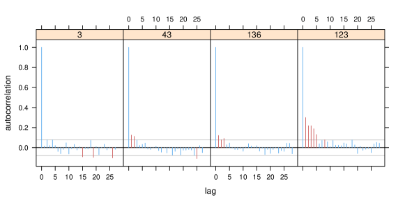
Figure 13: Autocorrelation functions for four subjects in the full gamm fitted to the KKL data.

Figure 13 clarifies that the full gamm succeeded in further reducing the autocorrelations in the residuals. This reduction is due almost exclusively to the use of factor smooths, with only tiny amelioration by adding in the three-way interaction with Trial. This result is important for two reasons. First, it is unlikely that the removal of autocorrelation in the residuals could be accomplished by factor smooths fitting noise rather than signal. Likewise, it is unlikely that the huge reduction in aic when going from the linear mixed model to the gamm (2087, see Table 2) could be accomplished by just fitting noise. Second, the presence of slowly undulating processes in experimental data is a phenomenon that is itself of theoretical interest, and invites interpretation, clarification, and replication.

The remaining autocorrelations that are visible in Figure 13 are unlikely to be harmful, but to play safe, one might consider removing subject 123 from the dataset and refitting the model. Alternatively, these last remaining autocorrelations might be due to a simple ar(1) autocorrelative process in the errors, according to which the current error $e_{t}$ in the timeseries at time $t$ is equal to a proportion $\rho$ of the preceding error $e_{t-1}$ plus Gaussian noise $\epsilon_{t}$:

$$e_{t}=\rho e_{t-1}+\epsilon_{t},\text{ where }\epsilon_{t}\underset{\text{ind}}{\sim}N(0,\sigma^{2}).$$ (3)

Pinheiro and Bates, (2000) and Gałecki and Burzykowski, (2013) provide extensive discussion of how autocorrelation processes can be accounted for within the mixed modeling framework; Wood et al., (2015) provides technical details for gamms. With a mild proportionality constant $\rho=0.15$, autocorrelations are almost completely removed. Below, we will discuss the use of this parameter in more detail. Here, we note that models from which the factor smooths are removed, and for which $\rho$ is increased, provide substantially worse fits to the data, and fail to remove substantial autocorrelational structure at longer lags. This shows that the factor smooths may be essential for bringing under statistical control a substantial part of autocorrelative structure in experimental data.

Addressing the autocorrelation issue for the KKL data set does not lead to major changes in significances and magnitudes of fixed-effect coefficients and the magnitudes of the (significant) coefficients, as reported in Bates et al., (2015) and Kliegl et al., (2015). Nevertheless, the gamm offers enhanced insight into the data, specifically with respect to the effect of Orientation. In the reference model, the coefficient of this main effect was estimated at 0.041, with a standard error of 0.010 ($t=3.9$). However, in the full linear mixed effect model, the coefficient is smaller (0.014), comes with greater uncertainty (standard error 0.09), and is not significant ($t=1.5$). However, the final gamm estimates the coefficient at 0.039, with a standard error of 0.016 and a $t$ value of 2.491, reporting $p=0.013$. Furthermore, the interaction of Size by Orientation, which is significant in the lmm, is not significant in the gamm. Given the interaction of Trial by Orientation, the greater uncertainty about this main effect in the linear mixed model, and about the interaction with Size, makes sense. Furthermore, as expected, the variance of the conditional modes for the by-subject random effects of Orientation in the reference model is larger (by a factor two) than in the final gamm ($p<0.0001$, $F$-test). Again, this makes sense, as part of what originally looked like random noise linked to orientation can now be attributed to a learning effect over experimental time.

In summary, the KKL dataset is not sterile, but infected by the `human factor'. The by-subject time series are characterized by autocorrelated errors. Unlike particles in physics, or plots of barley in agricultural experiments, human subjects are intelligent beings whose behavior is not random over time, but adaptive. The present reanalysis shows that subjects adapt in different ways to the novel manipulation of canonical versus diagonal positioning of visual stimuli, which is a theoretically fertile result. This result is not available under one-size-fits-all mechanical model selection procedures based on the a-priori assumption that the data are sterile.

3.2 The baldey dataset

Our second example addresses the analysis of the response latencies elicited in the auditory lexical decision megastudy of Ernestus and Cutler, (2015) (data available at http://www.mirjamernestus.nl/Ernestus/Baldey/baldey_data.zip). Ernestus and Cutler include in their statistical analysis the reaction time to the preceding trial as a way of controlling for temporal dependencies in by-subject time series. As shown by Baayen and Milin, (2010), the inclusion of preceding reaction time successfully removes a considerable amount of autocorrelation in the residuals. Ernestus and Cutler also included Trial as a main effect, together with by-subject random slopes for Trial.

In what follows, we present an analysis of the reaction times of the baldey data, which shows that the human factor is even stronger in these data than suggested by the analyses of Ernestus and Cutler.

In our analysis — which is far removed from a ``comprehensive'' analysis of this rich data set — we departed from the analyses of Ernestus and Cutler in several ways. First, we analyzed an inverse transform of the reaction times (-1000/RT) rather than a logarithmic transform, as both graphical inspection and an analysis following Box and Cox, (1964) indicated the inverse transformation to better approximate normality.

Second, autocorrelations in the errors should not be brought under control by including preceding reaction time as a covariate. A statistical model with preceding reaction time as predictor is no longer a generating model, in the sense that it is no longer possible, given the model specification, to simulate the reaction times. We therefore explored by-subject factor smooths in combination with the possibility of an ar(1) process in the errors.

Third, we relaxed the assumption that effects would be the same across the two genders. There are indications that males and females may be differentially sensitive to word frequency (Ullman et al.,, 2002; Balling and Baayen,, 2008), but a gender by frequency interaction is not always found (Balling and Baayen,, 2012; Tabak et al.,, 2005, 2010). As the baldey data set combines a perfectly balanced set of subjects (10 males and 10 females) with a large number of items (2780 Dutch words), it provides a testing ground for differential effects of the two genders in lexical processing.

Finally, we relaxed linearity assumptions, replacing a strictly linear mixed model by a generalized additive mixed model.

The random effects structure of the model for the reaction times for words (see Table 5 in the appendix for a statistical summary) included random intercepts for word, as well as by-word random intercepts for gender. Different words enjoy different popularity across the genders (see also Baayen et al., 2016b, ), and adjusting by-word intercepts for gender results in a tighter model fit. With respect to subject, we included by-subject factor smooths for session. The data for this mega-study were collected over 11 sessions, and once by-subject factor smooths for session were included in the model, by-subject factor smooths for Trial became redundant. For subject, random slopes for the acoustic duration of the stimulus word were also well supported.

Lemma frequency (the summed frequency of a word's inflectional variants) revealed a non-linear effect that differed between females and males, as shown in the left and center panels of Figure 14. Females show a somewhat stronger frequency effect, as expected given the somewhat greater verbal skills of women compared to men (Kimura,, 2000) and replicating earlier results (Ullman et al.,, 2002; Balling and Baayen,, 2008). A novel finding is that the frequency effect appears linear for men, but shows a curvilinear pattern for women with little or no effect for very low and very high frequencies. Possibly, both the reduced slope and the simpler functional form of the male curve is tied in with the lesser verbal skills of men.

Furthermore, the effect of the acoustic duration of the auditory stimulus showed a small but statistically well-supported modulation by Trial, visualized in the right panel of Figure 14. About two-thirds through an experimental session, the effect of acoustic duration decreased somewhat. This can be seen by noticing the reduced gradient for (scaled) Trial equal to 0.5: the number of contour lines crossed when moving horizontally across the plot, i.e., for increasing acoustic duration, is smaller than early on in the experiment.

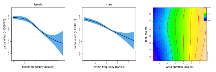
Figure 14: Interactions of Frequency by Gender (left and center panel), and of Word Duration by Trial (right panel), in the baldey data set. In the right panel, contour lines are 0.05 units apart (on the -1000/RT scale).

As for the KKL dataset, inclusion of session and trial in the model did not absorb all autocorrelation in the residuals. With $\rho=0.2$, the remaining autocorrelations were properly accounted for.

What this analysis shows is that subjects participating in an experiment with language materials bring with them their own experiences with the language, and that these specific experiences will lead to differentiated effects that for the baldey data set are partially differentiated by Gender. Furthermore, the effect of acoustic duration varied in the course of the experiment, providing further evidence for the human subject as a moving target (see also Ramscar et al.,, 2013; Baayen et al.,, 2015).

A strictly linear model provides an inferior fit to the baldey data (freml linear model: -13027.88, freml gamm: -14911.48, approximate test (informal because the models are not strictly nested): $\chi^{2}_{(4)}=1883.6,p<0.0001$). This linear model does not detect the interaction of frequency by gender. By imposing linearity, the nonlinear effect of frequency for females can only be accounted for by means of random intercepts and slopes, but the result is a model with a substantially worse goodness of fit. This example illustrates an important aspect of working with gamms: The model has to find the best balance between tracing variance back to random effects and tracing variance back to wiggly curves or (hyper)surfaces. This is why special care is required when carrying out model comparison, which we base on a comparison of freml scores using the chi-squared test, as implemented in the compareML function in the itsadug package for R.

We have seen, both for the KKL dataset and for the baldey dataset, that trial enters into significant interactions with predictors of interest. This raises the question of whether in the absence of such interactions, effects of trial are just a nuisance factor without theoretical interest. We think that even in such cases, exemplified for the baldey dataset by the factor smooth for session, are of more theoretical interest than one might think. Participants with more wiggly effects of session or trial are subjects with more variable responses. Ever since the study of Segalowitz and Segalowitz, (1993), it is known that more skilled and automatized processing is indexed by a lower coefficient of variation (cv, the ratio of the standard deviation and the mean of a subject's response times). For the baldey dataset, subjects' cv (calculated for the RTs to words, excluding short outlier RTs) and subjects' error proportions (calculated over all trials) enter into a strong negative correlation ($r=-0.64,t(18)=-3.6,p=0.0021$), indicating that subjects who are disproportionally less variable in their reaction times are the ones who make fewer errors (see also Segalowitz et al.,, 1999; Segalowitz and Hulstijn,, 2009). A greater variability in reaction times could be due to greater jitter on one hand, but also to greater fluctuations in attention and stronger effects of fatigue on the other hand. By-subject factor smooths for trial make visible this second source of subject variability, and are therefore diagnostic of differences in the degree to which language processing skills have been automatized.

3.3 The poems dataset

Our final example addresses a data set previously discussed by Baayen and Milin, (2010), available under the name poems in the RePsychLing package. This data set comprises a total of 275996 self-paced reading latencies from 326 subjects, for 2315 words appearing across 87 modern Dutch poems. Words are partially nested under poems. Any given subject read only a subset of poems.

Baayen and Milin included random intercepts for subject, word, and poem, as well as several by-subject and by-word random slopes for various numerical predictors. These authors sought to eliminate the problem of autocorrelated errors by including trial as a predictor, as well as the self-paced reading latency at the preceding word.

As discussed in detail by Bates et al., (2015), the model of Baayen and Milin is overparameterized with respect to its random effects structure. Given the Zipfian shape of word frequency distributions and the large numbers of words occurring only once in the corpus of poems, data are too sparse to include word as random-effect factor. Furthermore, correlation parameters for by-word random intercepts and slopes in the Baayen and Milin model were quite large, with absolute magnitudes $>0.8$, often an indicator of an overparameterized model. As for the baldey data discussed in the preceding section, including an ar(1) process in the errors is a principled and effective solution for addressing the issue of autocorrelated errors.

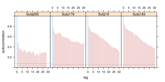
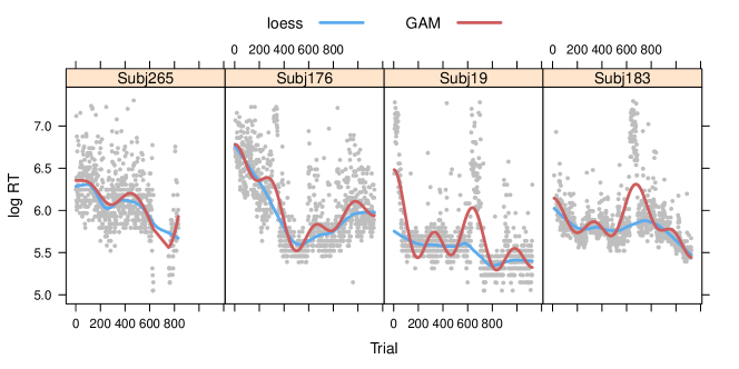
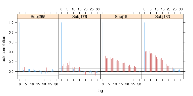
Figure 15: Autocorrelation functions for log reaction time for four exemplary subjects in the poems data set (upper panel), the corresponding plots (center panels) graphing log reaction time against trial, with a loess smoother (span = 0.2, in blue) and a gam factor smooth (red), and autocorrelations in the residuals of the gamm ($\rho=0.3$).

Within the context of the present discussion, the poems dataset is of interest for two reasons. First, because subjects are reading connected discourse rather than responding to unrelated isolated stimuli, the autocorrelation in their responses is much stronger than in the KKL and baldey datasets. This is illustrated in the top panels of Figure 15 for four exemplary subjects. In this dataset, there is only a handful of subjects without autocorrelations, and there are subjects with even stronger autocorrelations than the ones shown here. The second row of panels shows the corresponding scatterplots with loess and gam smoothers. Especially for subjects 19 and 183, there are temporally concentrated spikes of long reading times that are beyond what a gam smooth can capture. The lower set of panels illustrates the limitations of what the gamm fitted to this data set (and described in detail in Table 7 in the appendix) can accomplish. For subject 265, the autocorrelations are properly removed, and for subject 176, the reduction in autocorrelation is perhaps satisfactory. This is not the case for subjects 19 and 183, unsurprisingly given the spiky trends in the scatterplots.

Increasing $\rho$ is not an option. As discussed in further detail in Baayen et al., 2016b , since different subjects typically emerge with different degrees of autocorrelation, one would want to adjust the $\rho$ parameter for each individual subject. Unfortunately, it is at present not known how to achieve this mathematically within the framework of the generalized additive mixed model. As a consequence, the optimal $\rho$ is one that strikes a balance, such that the autocorrelation for subjects with strong autocorrelation is reduced as much as possible, without introducing artificial negative autocorrelation at short lags for subjects with little or no actual autocorrelation in their residuals.

Keeping in mind the caveat that the gamm provides an imperfect window on the complex quantitative structure of the poems data, it is of interest that word frequency appears to enter into a strong interaction with Trial. The appendix reports two models, one with a single multivariate smooth for these two predictors, and one in which their joint effect is decomposed into separate, additive, main effects of Trial, Frequency, and their interaction (see also Matuschek et al.,, 2015). These three partial effects are presented in Figure 16. We see a linear facilitatory main effect of (log-transformed) Frequency (left panel), a U-shaped effect of Trial (center panel), and an interaction that rides on top of these two main effects (right panel). The contour plot indicates that in the early trials, frequency had a more downward-sloping gradient. Later in the experiment, the effect of frequency is attenuated. The reduction in the magnitude of the frequency effect as the experiment proceeds makes sense. As subjects read through the poems selected for them, they tune in to this particular genre and its vocabulary. Words are repeated, and become more predictable as words align into sentences, and sentences into poems. As a consequence, frequency of occurrence as a contextless lexical prior becomes increasingly less informative.

Figure 16: Partial effects for Frequency and Trial in a gamm with an anova decomposition into additive main effects and interaction, for the poems data set.

We conclude with noting that all effects also receive generous support in a linear mixed effects model. Although this model lacks in precision (reml linear model: 150493.3, reml gamm: 49642.31; squared correlations of fitted and observed RTs 0.50 and 0.43 respectively), the linear mixed model offers an insight that is not easily gleaned from the generalized additive mixed model, namely, that the by-subject posterior modes for the intercept and the by-subject posterior modes for frequency are negatively correlated ($\hat{r}=-0.61$). A correlation parameter in the linear mixed model is well-supported by a likelihood ratio test ($p<0.0001$). Figure 17 presents the by-subject coefficients (obtained by adding the respective posterior modes to the population parameters) for intercept and frequency. The negative correlation is well visible, and indicates that a frequency effect is present only for those subjects who on average respond more slowly. This provides a further illustration that random effects are not necessarily just `nuisance parameters', but may provide insights that are of theoretical interest.

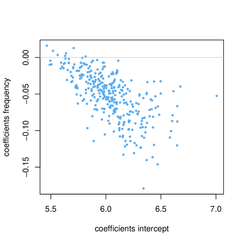
Figure 17: Estimated by-subject coefficients for intercept and frequency in a linear mixed model fitted to the self-paced reading latencies in the poetry data set. Slower subjects, which have larger intercepts, have more negative coefficients for frequency, whereas the faster responders (smaller intercepts) have coefficients for frequency close to zero.

4 Regression modeling strategies

We have presented three examples demonstrating interactions of the human factor with predictors of theoretical interest. This raises the question of how to proceed with the analysis of non-sterile experimental data. In what follows, we first address this question in the context of confirmatory (or hypothesis-testing) data analysis, and then turn to exploratory (or hypothesis-generating) data analysis.

4.1 Confirmatory data analysis

An excellent introduction to confirmatory multivariate data analysis is the monograph on regression modeling strategies by Harrell, (2015). For clarity of exposition, we simplify analytical reality and describe the analysis as proceeding in three discrete steps. During the first step, the data are validated and explored visually, the distributions of the response variables and the distributions of the predictors are inspected, and transformed where necessary (Box and Cox,, 1964). In the light of what has been learned from the initial survey of the data, including indications about non-linearities and the potential importance of covariates and possibly the presence of the human factor, a regression model can now be formulated. At the second step, the regression model is fitted to the data, and significance is assessed. This is the single and only time in the analytical process that a regression model is assessed. The third step proceeds with model criticism. At this stage, it is important to ascertain that the model fitted to the data at step 2 is indeed appropriate for the data. For a Gaussian regression model, for instance, it is important to verify that the residuals approximately follow a normal distribution, that they are independently and identically distributed, and that they do not show systematic variation with any predictors nor with the response variable. It is only when a critical term in a regression model withstands all attempts to bring it down with model criticism that one may conclude that there is reason to think that, given the simplifying assumptions that come with any regression model (see below for further discussion), a particular effect is actually supported. The size of the effect, compared to the effects of other predictors in the model, as well as the corresponding uncertainties associated with the parameter estimates, will be essential for the assessment of the scientific importance of this support. Importantly, the parameters in the model should be meaningful, at two levels. Mathematically, parameters should be properly estimable and interpretable. Furthermore, at the level of domain knowledge, all parameters should be theoretically interpretable. For instance, by-subject random intercepts in a regression model fitted to a reaction time study are interpretable as a random variable placing subjects on a scale from fast to slow responders, and by-subject factor smooths for experimental time are interpretable as reflecting the ebb and flow of attention.

Since a confirmatory analysis allows one, and only one, statistical test for the evaluation of a specific hypothesis, it is of crucial importance that this test is based on models that are not too complex to be estimable, on models that are properly interpretable, and on models that take the human factor into account if it is present. How then might one proceed under these stringent boundary conditions?

At first sight, it might be argued that a model should be fit to the data that is as complex as possible, a model that takes all possible contingencies into account that might put the critical model parameter in jeopardy. Thus, one might think that it is straightforward to enrich a maximal linear mixed model with predictors targeting the human factor. Unfortunately, once one enters the nonlinear world, this is even less advisable than for the linear world, for a variety of reasons.

First, more elaborate models can quickly become very difficult to understand. By way of example, a model with a four-way interaction of Word Duration, Session, Frequency and Trial improves substantially on the model presented above for the baldey data set ($\chi^{2}_{9}=24.35,p<0.0001$). But what we learn from this four-way tensor product is unclear. In 1959, Sigmund Koch wrote that ``Psychology [is] unique in the extent to which its institutionalization preceded its content and its methods preceded its problems.'' (Koch,, 1959, p. 783). Whereas this may not be true for all areas of psychological science (e.g., some areas of vision research), it certainly applies to the domain of lexical processing. Here, gamms will often be informative about possible structure in experimental data that is far beyond what current theories can explain or predict. For the baldey data, we deliberately avoid a `maximal' model, as, given current knowledge, it is unclear whether such a model would contribute to understanding the data.

Second, when we make use of a factor smooth with shrinkage to fit nonlinear by-subject trends over experimental time, we are making many simplifying assumptions, among which (i) that all subject smooths can be captured with the same smoothing parameter, and (ii) that these temporal trends do not interact with other predictors in the model, whether factorial (say, a priming condition) or metric (say, frequency or valence). These assumptions may or may not be valid, but it typically does not make much sense to aim for a complex model term such as a tensor product smooth for trial by frequency by valence by priming by subject, with or without shrinkage. Again, given our current state of knowledge, such complex models, if at all estimable, will typically be very difficult to interpret.

Third, fitting a complex generalized additive mixed model is not a trivial issue, and for results to be sensible, it is crucial to avoid random effects structure that is internally collinear (see Bates et al.,, 2015, for detailed discussion). In general, as observed by Wood (documentation for gam.selection in the mgcv package),

The more thought is given to appropriate model structure up front, the more successful model selection is likely to be. Simply starting with a hugely flexible model with `everything in' and hoping that automatic selection will find the right structure is not often successful.

Would researchers come to `wrong' conclusions if they analyze data simply using maximal linear models, without taking the human factor into account, without paying attention to whether the model is overfitting the data with mathematically uninterpretable parameters (Lele et al.,, 2012; Bates et al.,, 2015), and accepting less than nominal power (Matuschek et al.,, 2016)? The problem here is that low-hanging fruit is easily plucked, often by simple linear models without any random effects. The devil is in the details. Significance of factorial contrasts may not change, or may not change by much, when the human factor is taken into account. For the KKL data set, we showed that a full mixed model would lead to the conclusion that the main effect of Orientation is not significant, whereas a model that takes the human factor into account suggests otherwise. Furthermore, the maximal model suggests that the interaction of Size and Orientation is significant, but the gamm with predictors for the human factor indicates that there is no support whatsoever for such an interaction. Details change, but the three-way interaction of Orientation by Size by Gravitation remains. Do the details matter?

If details don't matter, in many cases the analyst will be well off with a simple linear model, even a linear model without random effects. Often, conclusions about `significance' do not change when data sets are analysed with much simpler models. However, when a simple linear model produces the same verdict on significance as a linear mixed model, or a linear mixed model provides the same verdict of significance as a generalized additive mixed model, this does not mean that the more complex modeling technique is not required. Even when conclusions about significance of predictors do not change for observed examples, they might change substantially for as yet unobserved examples. More importantly, random slopes and random intercepts typically modulate effect sizes and degrees of uncertainty. Especially when it comes to prediction, more precise estimates that take into account subject and item variability are invaluable. Similarly, taking into account nonlinearities and human factors may modulate conclusions about effect sizes and the precise nature of functional relations. For the KKL dataset, we observed a significant partial effect of Orientation, modulated by interactions with far smaller effect sizes. The partial effect of Orientation is of theoretical significance, and it therefore is important to use a modeling strategy that makes its partial effect visible.

Given that a maximal model approach provides the false security of a comfort blanket, the question remains how one might proceed under the stringent boundary conditions of confirmatory data analysis. All we can do to answer this question is present examples of how one might proceed. Consider a chronometric experiment with subjects and items. Inspired by Harrell, (2015), one possible way to proceed could be as follows. As a first step, following data validation, exploratory visualization is carried out. At this stage, non-parametric scatterplot smoothers could be used to probe for the presence of by-subject trends over experimental time. Furthermore, the autocorrelation function could be obtained for the response variable, in order to assess what value of $\rho$ might be required. However, because the temporal autocorrelation can be due to the combined presence of an ar(1) process in the errors and subject-specific trends in experimental time, the autocorrelation function for the response may overestimate the value of $\rho$ when by-subject trends in experimental time are in fact present. Therefore, it may be preferable to fit an intercept-only gamm with factor smooths for subject and random intercepts for item to the data, with as only aim to detect with more precision the extent to which the human factor is present, to determine whether it is necessary to include by-subject factor smooths, and to obtain an estimate for the autocorrelation parameter $\rho$. If there is no clear evidence for the human factor, a linear mixed model is an excellent choice, otherwise, a gamm is preferable, with an autocorrelation parameter for the ar(1) process in the errors set close to the autocorrelation at lag 1 observed for the intercept-only model.

Then, at step two of the analysis, a model could be fitted with all relevant fixed-effect parameters added in, but without any further random effects and random slopes. Significance of the critical predictor can now be assessed through model comparison with a simpler model from which the critical predictor, or the relevant critical interaction with this predictor, is removed. Importantly, this is the single and only time at which significance is assessed.

The final step proceeds to model criticism. At this step, the question is whether significance (if established) will survive removal of overly influential outliers, addition of further random-effect parameters (specifically, and importantly, random effects or random slopes for the critical model terms), adjustment of the autocorrelation parameter if necessary, and inclusion of interactions with human-factor variables. Bootstrap validation is also worth considering at this step. If an effect withstands model criticism, it can be reported as significant with the p-value obtained at step 2, otherwise, it should be reported as not significant. This confirmatory modeling strategy has the advantage that models that overfit the data with meaningless parameters are avoided. As pointed out by Lele et al., (2012), ``Whenever mixed models are used, estimability of the parameters should be checked before drawing scientific inferences or making management decisions''. Since meaningless parameters can arise even under convergence (see Bates et al.,, 2015), the analyst may want to minimize the risk of running into this situation specifically when significance is assessed in a confirmatory context.

Importantly, there are other strategies that could be followed, such as starting with a model including all random intercepts and all random effects and slopes, while leaving out correlation parameters (Bates et al.,, 2015). Here, a confirmatory setting takes the significance of the pertinent predictor as the outcome of interest, and subsequent model criticism is carried out to ensure that this significance is trustworthy. If it turns out that the model is too complex to be supported by the data, the analyst may want to refit a simpler and better justified model, in which case the analysis has become exploratory — it is only as long as significance is evaluated once, and once only, with subsequent model criticism to ensure support for the original significance test, that the analysis is a proper confirmatory analysis. What specific strategy is followed, and we have given only two of many possible strategies, is, to a large extent, a matter of taste, so it would make sense to report the details of the strategy that was actually followed for a given confirmatory analysis. In any case, the most transparent way to proceed is to release all data and code with the published paper, so that readers have the option to draw their own conclusions from the data.

4.2 Exploratory data analysis

One of the causes of the deplorable rate of replication failure for psychology (and many other fields of inquiry) is that confirmatory data analysis is seen as vastly superior to exploratory data analysis, and that as a consequence, the results of many exploratory data analyses are presented as if they were the result of confirmatory analysis.

All models reported in the present study are the result of data exploration with step-by-step theory-driven incremental model building (for examples of such an approach, see Pinheiro and Bates,, 2000; González et al.,, 2014). The t and p-values reported in the appendix, therefore, are indicators of surprise and should not be taken at face value as exact probabilities. (Note, however, that the crucial probabilities for the human factor are so small, often $<$2$e$-16, that they may be expected to survive substantial correction for multiplicity.) We believe that exploratory data analysis is of great importance for those domains of inquiry where explicit and mathematically precise theories are lacking. In these areas of inquiry, results of experiments can be completely opposite to what was expected, even though in hindsight, they may make perfect sense (see, e.g., the anti-frequency effect in Figure 5, for a computational model based on discriminative learning that captures this effect, see Pham and Baayen,, 2015). Importantly, in an exploratory setting, one can actually learn from the data, in a multivariate setting often in many dimensions simultaneously, instead of receiving only confirmation (or disconfirmation) of a single hypothesis.

Also in an exploratory setting, model criticism is absolutely essential. An effect is worth taking seriously only if it withstands truly serious attempts to bring it down. Researchers may want to complement exploratory regression analysis with techniques from machine learning such as random forests (Breiman,, 2001; Strobl et al.,, 2009) or gradient boosting machines (Friedman,, 2001; Chen et al.,, 2015) to obtain an independent assessment of variable importance that is orthogonal to the exploration of the data with regression modeling. These techniques are not plagued by issues of collinearity (Wurm and Fisicaro,, 2014), and they do not require any kind of model selection (for an example, see, e.g., Baayen et al., 2016a, , for application of random forests for this purpose).

4.3 A gold standard?

The Open Science Collaboration, (2015) reported the results of an extensive series of replication studies, and documented a 50% drop in observed effect sizes and a drop from 97% to 36% of significant results. Publication bias (Francis,, 2012), non-random selection of stimuli and subjects (Forster,, 2000; Sander and Sanders,, 2006; Francis,, 2013), societal changes (Ramscar et al.,, 2015) and especially lack of power (Button et al.,, 2013; Westfall et al.,, 2014) are major concerns. Clearly, many of the results in the published literature are but moving shadows of the true effects, which raises the question how to escape from the current methodological cave.

Barr et al., (2013) proposed a new standard for the statistical analysis of experimental data. Based on a series of simulation studies, they argued that anti-conservative p-values are best avoided by fitting linear mixed effects models with all variance components included that could in principle be non-zero given the experimental design. The simulations on which Barr et al., (2013) base their recommendation make very specific assumptions:

We assumed no list effect; that is, the particular configuration of `items' within a list did not have any unique effect over and above the item effects for that list. We also assumed no order effects, nor any effects of practice or fatigue. (p. 264)

Given our limited understanding of the human factor, this simplification is understandable. However, this very simplification invalidates their simulation design as a foundation for a general gold standard. We have shown that the human factor may interact with key predictors, and that it may lead to different conclusions about the details of their effects.

Since the proposed standard of Barr et al. is overly conservative with an unnecessary loss of power (Matuschek et al.,, 2016), and since it comes with the risk of basing conclusions on mathematically ill-defined models that overfit the data (Lele et al.,, 2012; Bates et al.,, 2015), Barr et al.'s proposal has the unfortunate side-effect of locking analytical practice in a methodological cage of shadows from which the true structure of experimental data, rich and fertile in perhaps unexpected ways, cannot be fully appreciated.

Recommendations such as the one of Barr et al., which once in the literature quickly rise to the status of rules enforced in the review process with an iron fist, have the unfortunate side effect of diverting attention from the model, the balance of forces within the model, the uncertainties associated with the model, and its inevitable weaknesses, to the so fervently desired but so over-valued p-value. A one-size-fits-all rule for obtaining such p-values might seem attractive as the only way to obtain an `objective' procedure evaluating experimental effects. However, irrespective of whether analysis is exploratory or confirmatory, in the modern age, objectivity can be achieved in a much more direct way. Whereas before the advent of the internet, reporting p-values in printed journals was the only way to make an argument that a particular effect is present, current communication technology makes it possible to publish not only p-values but the data themselves, using platforms such as the Mind Research Repository at http://openscience.uni-leipzig.de/index.php/mr2 or the Open Science Framework (https://osf.io/), where data can be made available together with details on the statistical analysis. With the data out in the open, readers will not only be able to evaluate for themselves the appropriateness of the analyses reported in a journal, but opportunities are created for improved analyses, either with current or with future statistical software. In this way, a degree of objectivity can be reached that goes far beyond what can be obtained by mechanical procedures and the considerable risk of associated artifacts. Furthermore, through meta-analysis, one can build on previous findings.

5 Discussion

Even though there is considerable awareness in the literature on memory and language that time series of behavioral responses are not independent (Broadbent,, 1971; Welford,, 1980; Sanders,, 1998; Taylor and Lupker,, 2001; De Vaan et al.,, 2007; Baayen and Milin,, 2010; Masson and Kliegl,, 2013), the fact that this interdependence has far-reaching consequences for the statistical analysis of experimental data has not received systematic reflection. We have reported three data sets in which inter-trial dependencies are present. Unlike molecules or barley, the units from which response variables in psychology are harvested are intelligent beings that constantly adapt to their environment. Humans learn. They get tired. Their attention wanes, and then is refocused on the task. When attentional and adaptative processes are demonstrably present in experimental data, and interact with predictors of theoretical interest, it is advisable to bring these processes under statistical control. Failure to take the human factor into consideration comes with the risk of misunderstanding the finer details of the quantitative structure of the data and the extent to which this structure is shaped by the predictors of interest.

We have introduced the generalized additive mixed model as an extension of the linear mixed model that makes it possible to bring the human factor into the statistical model, and to take the statistical sting out of the autocorrelations in the residual error. We do not wish to claim that with gamms researchers will finally emerge from the cave of shadows and apprehend the true effects themselves. But we are finding gamms helpful in sharpening the contours and outlines of these effects. For almost all data sets that we have investigated with gamms, we have obtained better fits by including by-subject factor smooths for trial. We also demonstrated interactions of trial with predictors of interest, a first step towards a better understanding of the human factor in lexical processing.

As any statistical model, gamms build on assumptions that are hoped to be reasonable, but of which we often know they involve substantial simplifications. When using gamms, it is important to have good coverage of the covariate space, especially when using generalized models with Poisson or binomial families, and highly irregular regression surfaces with highly localized effects should be treated with caution. Unlike the linear mixed model, the gamm as implemented in the mgcv package does not offer the possibility to test for correlation parameters in the random effects. Analysts used to the speed with which the software of the fourth author fits lmms will find the speed with which gamms with complex random effects structure converge excruciatingly slow, the price paid for not imposing prior constraints on the random effects structure. Furthermore, the penalized factor smooths that we have used assume a common smoothing parameter for all subjects, which may be true, but may also be incorrect. The factor smooths build on spline theory, but when time series of reaction times are spiky instead of smoothly wiggly, splines are better than nothing, but certainly not perfect. To this list of limitations we can also add that the adjusting of the errors for an ar(1) autocorrelative process will often be too simplistic in two ways. First, as we have demonstrated, $\rho$ should ideally vary with participant, which is currently not possible with the gam (and bam) functions of the mgcv package (but progress may be possible here by going fully Bayesian, see Wood, 2016). Second, there is no guarantee that the autocorrelative process is a simple ar(1) process — dependencies may well stretch further back in time. Nevertheless, we believe that with gamms, researchers have a tool in hand with which the real-life complexities with which psycholinguistic data may be infected can start to be investigated.

We conclude with some reflections on parsimony in regression modeling. George Box is well known for stating that all models are wrong, but that some are useful (Box,, 1979). With respect to model parsimony, he noticed that

Since all models are wrong the scientist cannot obtain a ``correct'' one by excessive elaboration. On the contrary following William of Occam he should seek an economical description of natural phenomena. Just as the ability to devise simple but evocative models is the signature of the great scientist so overelaboration and overparameterization is often the mark of mediocrity. (Box,, 1976, p. 792)

When working with gamms, models of considerable complexity can be fit to experimental data sets. Since language is a complex cognitive skill serving users interacting in highly complex and technologically advanced societies, it is perhaps not surprising that statistical models may need to be more complex than previously thought when it comes to taking into account the human factor. Within the boundary conditions of not overparameterizing, of properly balancing Type I and Type II error rates, and of having a model with meaningful and interpretable parameters, the challenge is to find the right balance between model simplicity and faithfulness to the data.

Within the context of confirmatory data analysis, a possible modeling strategy might be to keep the model lean, with factor smooths and an autocorrelation parameter included when there appears to be evidence for the human factor, and to shift the burden of securing a reasonable degree of confidence about a critical effect to model criticism. It must be acknowledged that an important achievement of the Barr et al., (2013) paper was to raise awareness about the dangers of fitting overly simple linear mixed models. However, their recommendation (summarized in the title of their paper) to ``keep it maximal'', crosses over to such an extreme position as to be untenable in most realistic statistical modeling settings.

Within the context of exploratory data analysis, incremental hypothesis-driven model building can yield an accumulation of valuable insights. Importantly, theory and experience should guide model building, counterbalancing faithfulness to the data with a drive for simplicity. For the KKL data set, for instance, the three-way interaction of Orientation by Size by Trial was explored because we thought it was conceivable that within-experiment learning and adaptation might vary with the difficulty of the different testing conditions. It is possible that the details of this interaction vary from subject to subject. Without hypotheses about what might drive individual differences in a four-way interaction with subject, such an interaction, even if it were estimable, would be extremely difficult to understand. For the baldey data set, we considered the possibility that listeners might adapt to the speech rate of the speaker as the experiment proceeded. However, we refrained from discussing a model in which Trial and Word Duration entered into further interactions with Session and Frequency, even though such a four-way interaction, which is estimable, improves substantially on the model presented above for the baldey data. This more complex model might be capturing something real, but without guidance from theory, and without further support from replication studies, it is unclear what the benefits of such a complex model might be. For the poetry data set, the model reported in Baayen and Milin, (2010) turned out to be overparameterized, the data for words being too sparse to allow inclusion of by-word random intercepts and slopes. Therefore, our gamm for the poetry data did not include random effects for words. In short, also in the context of exploratory data analysis, parsimony is a virtue, not a vice.

The probability of objectivity and replicability in data analysis, whether exploratory or confirmatory, is likely to be enhanced when researchers make their data and analyses available to the research community. Of course, making data available does not protect against experimental fishing expeditions, such as running additional subjects until significance is obtained, or running a pilot study and selecting for the main experiment that subset of items that in the pilot study yielded the desired effect. Transparency in reportage is therefore also of great importance. However, just by itself, making the data available is a substantial deterrent for reporting results of fishing expeditions: Anyone with access to the data will immediately spot that the model published is an implausible one. Publication of data will also render fishing expeditions across multiple methods for analyzing the data less attractive. For instance, reporting an F1+F2 analysis (Forster and Dickinson,, 1976) that supports significance after first having observed a lack of significance in a lmm is straightforward to detect. Rather than seeking to guarantee objectivity through rigid methodological one-size-fits-all prescriptions, we think open science, combined with responsible statistical analysis, is the way forward out of the cave of shadows.

Notes

1. 1 For a fully Bayesian approach to generalized additive modeling, see Wood, (2016), where an interface between mgcv and the bugs language is discussed. With this interface, it becomes possible to adopt a fully Bayesian approach to GAMMs.
2. 2 In the gamm framework, random effects can be thought of as smooths with a zero-dimensional null space, i.e., as splines with no completely smooth basis functions (such as the first two basis functions in Figure 3). At the same time, the prior on wiggliness is equivalent to the requirement that the coefficients of the smooth ($\bm{\beta}$) follow a multivariate normal distribution with zero mean. In other words, they can be viewed as a source of Gaussian noise, just as the random effects in the linear mixed model.
3. 3 Except for the baldey dataset, which is available on-line as documented below, all data sets discussed are available in the RePsychLing package for R. Detailed R code for the analyses reported is available in this package in the folder inst as caveOfShadows.pdf, and at http://www.sfs.uni-tuebingen.de/~hbaayen/publications/supplementCave.pdf.
4. 4 Given the small number of sessions (11) and the large number of observations for each session (around 4500 for each subject), one could opt for treating session as a factor, and including by-subject random slopes for this factor. Results are very similar, with the factor smooths showing slightly more shrinkage.
5. 5 Including the previous reaction time as covariate in order to reduce the autocorrelation in the error, as suggested by Baayen and Milin, (2010), has many disadvantages compared to including an ar(1) process in the errors, and is not recommended.
6. 6 It might be argued we have not shown that addressing autocorrelated errors changes conclusions about the effect of Orientation. The argument runs as follows. The main effect of a predictor $X$ that interacts with a predictor $Y$ specifies the effect of $X$ when $Y=0$. Since Orientation interacts with Trial, the main effect of Orientation specifies its effect when Trial = 0 (i.e., in the middle of the experiment, since Trial was scaled). From this, it would follow that we have no case to argue that it is the explicit treatment of autocorrelated errors that has changed the apparent conclusions from the model about the effect of Orientation. This argument misses three important points. First, autocorrelation in the errors is addressed in part by the by-subject factor smooths for Trial, and in part by the autocorrelation parameter $\rho$. It is the combination of the two that leads to different conclusions about the effect of Orientation. Second, as explained in section 2, main effects in a model with interactions are crucial for properly calibrating the wiggly curves for individual factor levels with respect to the intercept. They are an essential part of the model. Changing orientation from cardinal to diagonal implies a modulation of the intercept by 0.078 units on the -1000/RT scale. This change effects all trials for the relevant factor level. A maximal lmm estimates the effect to be much smaller (0.028) and not significant. In other words, the maximal lmm underestimates the distance between the relevant curves. Third, as a consequence, the maximal lmm provides a warped perspective of the magnitude of the effect of Orientation vis-à-vis the other predictors in the model.
7. 7 The review process forced a presentational style on this study in which the experimental results are reported as being predicted by discriminative learning theory, whereas the unexpected experimental results preceded in time the subsequent modeling with discriminative learning.
8. 8 Gams do not require especially large data sets. Examples from Wood, (2006) include a data set with only 31 observations on girth, height, and volume for black cherry trees, where a thin plate regression spline for girth appears justified, and a data set with 634 observations on mackerel eggs where a thin plate regression spline for longitude and latitude is part of the model specification. Of course, when there is only a handful of distinct values for a given covariate, a smooth for that covariate will not make sense. The smoothers in the mgcv package typically produce an error message for such cases.

Acknowledgements
 
This research was supported by an Alexander von Humboldt Professorship awarded to the first author. We are indebted to Simon Wood for invaluable discussion and feedback and for the many extensions he added to the mgcv package to facilitate the analysis of (psycho)linguistic data.

Appendix

The KKL dataset

random effects
 
Groups Name Std.Dev. Corr subj Intercept 0.161766 Trial 0.051180 -0.273 subj.1 spt 0.066809 subj.2 grv 0.033814 subj.3 obj 0.025609 subj.4 orn 0.076247 subj.5 spt_orn 0.033226 Residual 0.185591

fixed effects
 
Estimate Std. Error $t$ value Intercept 5.659 0.018 322.91 sze 0.184 0.035 5.27 spt 0.074 0.008 9.62 obj 0.043 0.005 9.41 grv -0.001 0.005 -0.17 orn 0.014 0.009 1.51 Soa L -0.010 0.001 -12.56 Soa Q 0.019 0.001 20.61 sze:spt 0.048 0.015 3.14 sze:obj -0.012 0.009 -1.30 sze:grv -0.037 0.010 -3.66 sze:orn 0.039 0.018 2.20 spt:orn 0.020 0.006 3.12 obj:orn 0.009 0.007 1.26 grv:orn 0.011 0.007 1.52 sze:spt:orn -0.014 0.013 -1.10 sze:obj:orn -0.003 0.014 -0.24 sze:grv:orn -0.047 0.014 -3.25 Trial L -0.043 0.006 -7.47 Trial Q 0.015 0.001 16.96 sze:Trial 0.018 0.011 1.60 orn:Trial 0.028 0.003 8.64 sze:TrialQ -0.000 0.002 -0.05 orn:TrialQ -0.006 0.005 -1.27

Table 3: Summary of the LMM fitted to the KKL data set. Extensions to the reference model are highlighted. For factors, $-$0.5/$+$05 dummy coding was used. L: linear, Q: quadratic.

A. parametric coefficients	Estimate	Std. Error	t-value	p-value
Intercept	5.6851	0.0189	300.4450	$<$ 0.0001
sze	0.1840	0.0378	4.8608	$<$ 0.0001
spt	0.0729	0.0079	9.2050	$<$ 0.0001
obj	0.0411	0.0041	9.9844	$<$ 0.0001
grv	-0.0005	0.0049	-0.1003	0.9201
orn	0.0375	0.0142	2.6441	0.0082
sze:spt	0.0483	0.0158	3.0453	0.0023
sze:obj	-0.0088	0.0082	-1.0749	0.2824
sze:grv	-0.0366	0.0099	-3.7074	0.0002
sze:orn	0.0096	0.0283	0.3375	0.7357
spt:orn	0.0213	0.0064	3.3449	0.0008
obj:orn	0.0083	0.0068	1.2129	0.2252
grv:orn	0.0078	0.0068	1.1387	0.2548
sze:spt:orn	-0.0098	0.0128	-0.7668	0.4432
sze:obj:orn	-0.0075	0.0136	-0.5502	0.5822
sze:grv:orn	-0.0483	0.0137	-3.5241	0.0004
B. smooth terms	edf	Ref.df	F-value	p-value
fs(Trial,subj)	557.8665	774.0000	661.8472	$<$ 0.0001
re(subj,spt)	77.7931	86.0000	31.5911	$<$ 0.0001
re(subj,grv)	47.6056	84.0000	2.1643	$<$ 0.0001
re(subj,obj)	29.5712	84.0000	1.3404	0.0011
re(subj,orn)	44.0796	84.0000	1.1481	$<$ 0.0001
re(subj,spt_orn)	47.3734	84.0000	1.3153	$<$ 0.0001
s(Trial): big+cardinal	8.3489	8.6794	13.4016	$<$ 0.0001
s(Trial): small+cardinal	8.0534	8.4887	9.8373	$<$ 0.0001
s(Trial): big+diagonal	5.8875	6.5738	5.8564	$<$ 0.0001
s(Trial): small+diagonal	7.9974	8.4525	8.8624	$<$ 0.0001
s(Soa)	5.6017	6.7468	103.1147	$<$ 0.0001

Table 4: Summary of the full gamm fitted to the KKL data set. Extensions to the reference model are highlighted. For factors, $-$0.5/$+$05 dummy coding was used. A separate factor was defined with four levels, one for each combination of Size and Orientation, and a thin plate regression spline (s()) was fitted for each of its four levels. re(X,Y) denotes random intercepts in $Y$ for grouping factor $X$. The penalized factor smooth for subject (fs(Trial, subj) includes by-subject intercept calibration.

The baldey dataset

	Estimate	Std. Error	t value	Pr($>$$|$t$|$)
Intercept	-0.96	0.04	-22.47	$<$ 0.0001
gender=male	0.21	0.06	3.49	$<$ 0.0001
	edf	Ref.df	F	p-value
s(LemmaFreq):gender=female	3.20	3.61	53.51	$<$ 0.0001
s(LemmaFreq):gender=male	2.26	2.51	52.23	$<$ 0.0001
te(word duration,Trial)	8.82	10.56	22.17	$<$ 0.0001
re(word)	1734.42	2777.00	2.03	$<$ 0.0001
re(word,gender)	495.12	5544.00	0.11	$<$ 0.0001
re(subject, word duration)	18.75	19.00	79.19	$<$ 0.0001
fs(session,subject)	154.36	178.00	143.62	$<$ 0.0001

Table 5: Summary of the model fit to the inverse transformed auditory lexical decision latencies in the baldey megastudy ($\rho=0.2$). Factors received treatment dummy coding, s() denotes a thin plate regression spline, and te() a tensor product smooth. re(X) denotes random intercepts for grouping factor $X$, and re(X,Y) specifies random slopes for $Y$ for grouping factor $X$. fs() denotes a penalized factor smooth. Frequency, word duration, and trial were scaled.

A. parametric coefficients	Estimate	Std. Error	$t$-value	$p$-value
Intercept	-0.94	0.04	-23.22	$<$ 0.0001
gender = male	0.24	0.06	4.14	$<$ 0.0001
LemmaFreq	-0.02	0.00	-12.54	$<$ 0.0001
word duration	0.06	0.01	8.75	$<$ 0.0001
Trial	0.01	0.00	7.44	$<$ 0.0001
gendermale : LemmaFreq	0.00	0.00	1.38	0.1684
word duration : Trial	-0.01	0.00	-6.44	$<$ 0.0001
B. smooth terms	edf	Ref.df	$F$-value	$p$-value
s(word)	1668.12	2777.00	2.79	$<$ 0.0001
s(gender, word)	451.77	5544.00	0.10	$<$ 0.0001
s(subject)	17.93	18.00	900901.26	$<$ 0.0001
s(word duration, subject)	18.74	19.00	121.38	$<$ 0.0001
s(session, subject)	19.90	20.00	717027.82	$<$ 0.0001

Table 6: Summary of a model for the baldey auditory lexical decision latencies with only linear effects. Frequency, word duration, and trial were scaled.

The poems dataset

	Estimate	Std. Error	$t$-value	Pr($>$$|$t$|$)
Intercept	6.05	0.02	347.71	$<$ 0.0001
	edf	Ref.df	$F$	$p$-value
te(Fre,Trial)	10.29	11.40	80.59	$<$ 0.0001
re(Poem)	81.19	87.00	19.45	$<$ 0.0001
fs(Trial, Subject)	2163.53	2934.00	329.42	$<$ 0.0001
re(Subject, Fre)	304.11	326.00	14.88	$<$ 0.0001

Table 7: Summary of the generalized additive mixed model fitted to the poems data, with $\rho=0.3$, and a tensor product smooth for Frequency by Trial (freml 49300). te(X,Y) denotes a tensor product smooth, re(X) random intercepts for grouping factor $X$, re(X,Y) denotes random slopes for $Y$ by grouping factor $X$, and fs() denotes a penalized factor smooth.

Figure 18: Tensor product smooth for the interaction of Frequency by Trial in the poems data set. In the left panel, green dotted lines indicate $+1$ standard error contour lines, and red dashed lines $-1$ standard error contour lines.

	Estimate	Std. Error	$t$-value	Pr($>$$|$t$|$)
Intercept	6.05	0.02	347.38	$<$ 0.0001
	edf	Ref.df	$F$	$p$-value
ti(Fre)	1.57	1.88	247.87	$<$ 0.0001
ti(TrialSc)	3.90	3.91	90.92	$<$ 0.0001
ti(Fre,TrialSc)	8.05	10.19	9.93	$<$ 0.0001
re(Poem)	81.18	87.00	19.41	$<$ 0.0001
fs(TrialSc, Subject)	2163.63	2934.00	323.82	$<$ 0.0001
re(Subject, Fre)	304.08	326.00	14.87	$<$ 0.0001

Table 8: Summary of a generalized additive mixed model fitted to the poems data, with additive effects of Frequency, Trial, and their interaction, and with $\rho=0.3$ (freml: 49300). ti(X,Y) denotes an independent tensor product smooth interaction term, and ti(X) the independent main effect of $X$. re(X) specifies random intercepts for grouping factor $X$, and re(X,Y) denotes random slopes for $Y$ by grouping factor $X$. fs() represents a penalized factor smooth, which absorbs the by-subject random intercepts.

Random effects
Groups	Name	Variance	Std.Dev	Corr
Subject	Intercept	0.0596	0.2441
	FreSc	0.0012	0.0343	-0.61
	TrialSc	0.0096	0.0981	0.01	0.04
Poem	Intercept	0.0025	0.0503
Residual		0.0994	0.3153
Number of obs: 275996, groups: Subject, 326; Poem, 87

Fixed effects
	Estimate	Std. Error	t value
Intercept	6.0390	0.0146	414.3
FreSc	-0.0526	0.0020	-26.3
TrialSc	-0.0783	0.0055	-14.3
FreSc:TrialSc	0.0039	0.0006	6.3

Table 9: Summary of a linear mixed model fitted to the poems data.

References

- Arnon and Ramscar, (2012) Arnon, I. and Ramscar, M. (2012). Granularity and the acquisition of grammatical gender: How order-of-acquisition affects what gets learned. Cognition, 122(3):292–305.
- Baayen and Milin, (2010) Baayen, R. H. and Milin, P. (2010). Analyzing reaction times. International Journal of Psychological Research, 3:12–28.
- (3) Baayen, R. H., Milin, P., and Ramscar, M. (2016a). Frequency in lexical processing. Aphasiology.
- Baayen et al., (2015) Baayen, R. H., Tomaschek, F., Gahl, S., and Ramscar, M. (2015). The Ecclesiastes principle in language change. In Hundt, M., Mollin, S., and Pfenninger, S., editors, The changing English language: Psycholinguistic perspectives, page to appear. Cambridge University Press, Cambridge, UK.
- (5) Baayen, R. H., van Rij, J., de Cat, C., and Wood, S. N. (2016b). Autocorrelated errors in experimental data in the language sciences: Some solutions offered by generalized additive mixed models. In Speelman, D., Heylen, K., and Geeraerts, D., editors, Mixed Effects Regression Models in Linguistics, page to appear. Springer, Berlin.
- Balling and Baayen, (2008) Balling, L. and Baayen, R. H. (2008). Morphological effects in auditory word recognition: Evidence from Danish. Language and Cognitive Processes, 23:1159–1190.
- Balling and Baayen, (2012) Balling, L. and Baayen, R. H. (2012). Probability and surprisal in auditory comprehension of morphologically complex words. Cognition, 125:80–106.
- Barr et al., (2013) Barr, D. J., Levy, R., Scheepers, C., and Tily, H. J. (2013). Random effects structure for confirmatory hypothesis testing: Keep it maximal. Journal of Memory and Language, 68(3):255–278.
- Bates et al., (2015) Bates, D., Kliegl, R., Vasishth, S., and Baayen, R. H. (2015). Parsimonious mixed models.
- Box, (1976) Box, G. E. P. (1976). Science and statistics. Journal of the American Statistical Association, 71:791–799.
- Box, (1979) Box, G. E. P. (1979). Robustness in the strategy of scientific model building. In Launer, R. L. and Wilkinson, G. N., editors, Robustness in Statistics, pages 201–236. Academic Press.
- Box and Cox, (1964) Box, G. E. P. and Cox, D. R. (1964). An analysis of transformations (with discussion). Journal of the Royal Statistical Society B, 26:211–252.
- Breiman, (2001) Breiman, L. (2001). Random forests. Machine Learning, 45:5–32.
- Broadbent, (1971) Broadbent, D. (1971). Decision and Stress. Accademic Press, New York.
- Button et al., (2013) Button, K. S., Ioannidis, J. P., Mokrysz, C., Nosek, B. A., Flint, J., Robinson, E. S., and Munafò, M. R. (2013). Power failure: Why small sample size undermines the reliability of neuroscience. Nature Reviews Neuroscience, 14(5):365–376.
- Chen et al., (2015) Chen, T., He, T., and Benesty, M. (2015). xgboost: eXtreme Gradient Boosting. (R package version 0.4-0).
- Cleveland, (1979) Cleveland, W. S. (1979). Robust locally weighted regression and smoothing scatterplots. Journal of the American Statistical Association, 74:829–836.
- De Vaan et al., (2007) De Vaan, L., Schreuder, R., and Baayen, R. H. (2007). Regular morphologically complex neologisms leave detectable traces in the mental lexicon. The Mental Lexicon, 2:1–23.
- Dery and Pearson, (2015) Dery, J. E. and Pearson, H. (2015). On experience-driven semantic judgments: A case study on the oneiric reference constraint. In Proceedings of Quantitative Investigations in Theoretical Linguistics, Tübingen, 2015.
- Egly et al., (1994) Egly, R., Driver, J., and Rafal, R. D. (1994). Shifting visual attention between objects and locations: Evidence from normal and parietal lesion subjects. Journal of Experimental Psychology: General, 123:161–177.
- Ernestus and Cutler, (2015) Ernestus, M. and Cutler, A. (2015). BALDEY: A database of auditory lexical decisions. The Quarterly Journal of Experimental Psychology, (ahead-of-print):1–20.
- Forster, (2000) Forster, K. (2000). The potential for experimenter bias effects in word recognition experiments. Memory & Cognition, 28:1109–1115.
- Forster and Dickinson, (1976) Forster, K. and Dickinson, R. (1976). More on the language-as-fixed effect: Monte-Carlo estimates of error rates for F1, F2, F', and F'. Journal of Verbal Learning and Verbal Behavior, 15:135–142.
- Francis, (2012) Francis, G. (2012). Publication bias and the failure of replication in experimental psychology. Psychonomic Bulletin & Review, 19(6):975–991.
- Francis, (2013) Francis, G. (2013). Publication bias in ``Red, Rank, and Romance in Women Viewing Men'' by Elliot et al. (2010). Journal of Experimental Psychology: General, 142(1):292–296.
- Friedman, (2001) Friedman, J. H. (2001). Greedy function approximation: A gradient boosting machine. Annals of Statistics, 29(5):1189–1232.
- Gałecki and Burzykowski, (2013) Gałecki, A. and Burzykowski, T. (2013). Linear mixed-effects models using R: A step-by-step approach. Springer Science & Business Media.
- Gilden, (2001) Gilden, D. L. (2001). Cognitive emissions of noise. Psychological Review, 108:33–56.
- Gilden et al., (1995) Gilden, D. L., Thornton, T., and Mallon, M. W. (1995). noise in human cognition. Science, 267:1837–1839.
- González et al., (2014) González, B., De Boeck, P., Tuerlinckx, F., et al. (2014). Linear mixed modelling for data from a double mixed factorial design with covariates: A case-study on semantic categorization response times. Journal of the Royal Statistical Society: Series C (Applied Statistics), 63(2):289–302.
- Harrell, (2015) Harrell, F. (2015). Regression modeling strategies: with applications to linear models, logistic and ordinal regression, and survival analysis. Springer.
- Hastie and Tibshirani, (1990) Hastie, T. and Tibshirani, R. (1990). Generalized Additive Models. Chapman & Hall, London.
- James et al., (2013) James, G., Witten, D., Hastie, T., and Tibshirani, R. (2013). An introduction to statistical learning, volume 6. Springer.
- Kimura, (2000) Kimura, D. (2000). Sex and Cognition. The MIT Press, Cambridge, MA.
- Kleinschmidt and Jaeger, (2015) Kleinschmidt, D. F. and Jaeger, T. F. (2015). Robust speech perception: Recognize the familiar, generalize to the similar, and adapt to the novel. Psychological Review, 122(2):148.
- Kliegl et al., (2015) Kliegl, R., Kuschela, J., and Laubrock, J. (2015). Object orientation and target size modulate the speed of visual attention. Manuscript, University of Potsdam.
- Kliegl et al., (2011) Kliegl, R., Wei, P., Dambacher, M., Yan, M., and Zhou, X. (2011). Experimental effects and individual differences in Linear Mixed Models: Estimating the relationship between spatial, object, and attraction effects in visual attention. Frontiers in Psychology, 1:1–12.
- Koch, (1959) Koch, S. E. (1959). Psychology: A study of a science. McGraw-Hill.
- Lele et al., (2012) Lele, S. R., Nadeem, K., and Schmuland, B. (2012). Estimability and likelihood inference for generalized linear mixed models using data cloning. Journal of the American Statistical Association.
- Lin and Zhang, (1999) Lin, X. and Zhang, D. (1999). Inference in generalized additive mixed models using smoothing splines. JRSSB, 61:381–400.
- Marra and Wood, (2012) Marra, G. and Wood, S. N. (2012). Coverage properties of confidence intervals for generalized additive model components. Scandinavian Journal of Statistics, 39:53–74.
- Marsolek, (2008) Marsolek, C. J. (2008). What antipriming reveals about priming. Trends in Cognitive Science, 12(5):176–181.
- Masson and Kliegl, (2013) Masson, M. E. and Kliegl, R. (2013). Modulation of additive and interactive effects in lexical decision by trial history. Journal of Experimental Psychology: Learning, Memory, and Cognition, 39(3):898.
- Matuschek et al., (2015) Matuschek, H., Kliegl, R., and Holschneider, M. (2015). Smoothing spline ANOVA decomposition of arbitrary splines: An application to eye movements in reading. PLoS ONE, 10(3).
- Matuschek et al., (2016) Matuschek, H., Kliegl, R., Vasishth, S., Baayen, R. H., and Bates, D. (2016). Balancing Type I Error and Power in Linear Mixed Models. Journal of Memory and Language, page accepted pending minor revision.
- Mulder et al., (2014) Mulder, K., Dijkstra, T., Schreuder, R., and Baayen, R. H. (2014). Effects of primary and secondary morphological family size in monolingual and bilingual word processing. Journal of Memory and Language, 72:59–84.
- Nychka, (1988) Nychka, D. (1988). Bayesian confidence intervals for smoothing splines. Journal of the American Statistical Association, 83:1134–1143.
- Open Science Collaboration, (2015) Open Science Collaboration (2015). Estimating the reproducibility of psychological science. Science, 349(6251):aac4716.
- Pham and Baayen, (2015) Pham, H. and Baayen, R. H. (2015). Vietnamese compounds show an anti-frequency effect in visual lexical decision. Language, Cognition, and Neuroscience, 30(9):1077–1095.