Reduced bispectrum seeded by helical primordial magnetic fields

Héctor Javier Hortúa    Leonardo Castañeda
Abstract

In this paper, we investigate the effects of helical primordial magnetic fields (PMFs) on the cosmic microwave background (CMB) reduced bispectrum. We derive the full three-point statistics of helical magnetic fields and numerically calculate the even contribution in the collinear configuration. We then numerically compute the CMB reduced bispectrum induced by passive and compensated PMF modes on large angular scales. There is a negative signal on the bispectrum due to the helical terms of the fields and we also observe that the biggest contribution to the bispectrum comes from the non-zero IR cut-off for causal fields, unlike the two-point correlation case. For negative spectral indices, the reduced bispectrum is enhanced by the passive modes. This gives a lower value of the upper limit for the mean amplitude of the magnetic field on a given characteristic scale. However, high values of IR cut-off in the bispectrum, and the helical terms of the magnetic field relaxes this bound. This demonstrates the importance of the IR cut-off and helicity in the study of the nature of PMFs from CMB observations.

1 Introduction

Recent observational evidence of intergalactic magnetic fields from γ𝛾\gamma-ray observations of blazars and constraints imposed by CMB power spectrum suggest the existence of magnetic fields created in the early Universe [1, 2, 3, 4, 5]. Interesting theoretical models have been proposed to explain generation processes which gave rise to this likely primordial field. Some of them are originated by causal requirements via cosmological phase transitions or by non-linear evolution of primordial density perturbations[6, 7, 8]; and the other ones could be generated during inflation, with them being the most appealing models due to the production of large-scale magnetic fields beyond the horizon scale [9, 10, 11, 12, 13, 14, 15, 16, 17, 18, 19, 20, 21, 22, 23, 24, 25, 26, 27, 28, 29]. Moreover, several additional attempts from string theory or extra dimensions have been done to generate the seed magnetic fields needed to be coherent on cosmological scales [30, 31, 32, 33]. One way to find out the process which gave rise to this field and determine its main features is by making theoretical predictions about the signatures in the CMB from primordial magnetic fields (PMFs) [34, 35, 36, 37, 43]. Indeed, some authors have shown that vector modes dominate all the temperature and polarization anisotropies for higher multipolar numbers while the scalar mode contribution is larger for lower l𝑙l [44, 45, 38]. Other effect of PMFs on the CMB comes from the non-Gaussian (NG) signals because its contribution to energy-momentum tensor is quadratic in the fields. The relevant NG signal from PMFs with an amplitude similar to the curvature turns out to be a feature that is important for constraining mean-field amplitude depending on what signal is induced by passive or compensated modes. Studies of NG signals via bispectrum on CMB have found upper limits of PMFs around 2222222-22 nG derived from scalar magnetic modes, and 3.2103.2103.2-10 nG derived from vector-tensor magnetic modes smoothed on a scale of 111 Mpc [47, 48, 49, 50, 51, 52, 53, 54, 55]. The Planck Collaboration also reported limits on the amplitude of B1Mpc<3subscript𝐵1𝑀𝑝𝑐3B_{1Mpc}<3nG for nB=2.9subscript𝑛𝐵2.9n_{B}=-2.9; B1Mpc<0.07subscript𝐵1𝑀𝑝𝑐0.07B_{1Mpc}<0.07nG for nB=2subscript𝑛𝐵2n_{B}=-2; and B1Mpc<0.04subscript𝐵1𝑀𝑝𝑐0.04B_{1Mpc}<0.04nG for nB=2subscript𝑛𝐵2n_{B}=2 from compensated modes; and B1Mpc<4.5subscript𝐵1𝑀𝑝𝑐4.5B_{1Mpc}<4.5nG for nB=2.9subscript𝑛𝐵2.9n_{B}=-2.9 from the passive-scalar mode [56]. PMFs have also been constrained by the POLARBEAR experiment, where they reported that the PMF amplitude from the two-point correlation functions is less than 3.9 nG at the 95% confidence level [57]. On the other hand, distinct signatures on the parity-odd CMB cross correlations would carry valuable clues about a primordial magnetic helicity. In fact, helical contribution in the field (in the perfect conductivity limit) has been widely studied because it produces efficient transference of power from smaller to larger scales, and thus be able to explain the actual observed magnetic fields[6, 58]. Further, observational evidence of helical primordial magnetic fields would offer a window for probing physics beyond the standard models of particle physics, particularly processes of parity violation in the early Universe[59, 60, 61].
The study of helical fields via NG will give a deeper understanding of the magnetic field generation model and help us to strengthen the constraints of PMF amplitude. Thus, the main goal of this paper is to investigate the effects of helical PMFs on the CMB bispectrum. Following previous formulation for calculating the bispectrum, we have found signals that arise by considering a minimal cut-off and we observed that local-type shape contains the biggest contribution to the bispectrum. This paper is organized as follows. Sec. 2 describes the statistical properties of PMFs. In Sec. 3 we define the magnetic bispectrum and in Sec.4 through the numerical computation, we solve exactly the bispectrum for a collinear configuration and observe some important signals. Sec. 5 is defined the reduced bispectrum and in Sec. 6 we present numerical results of the primary bispectrum sourced by helical PMFs. Sec. 7 is devoted to further discussion and conclusions.

2 Statistical Aspects of Primordial Magnetic Fields.

We consider a stochastic primordial magnetic field (PMF) generated in the very early Universe which could have been produced during inflation (non-causal field) or after inflation (causal field). This field acts like a source of fluctuations on the CMB anisotropies under a FLRW background Universe described by the metric

ds2=a2(t)(dt2+δijdxidxj)𝑑superscript𝑠2superscript𝑎2𝑡𝑑superscript𝑡2subscript𝛿𝑖𝑗𝑑superscript𝑥𝑖𝑑superscript𝑥𝑗ds^{2}=a^{2}(t)(-dt^{2}+\delta_{ij}dx^{i}dx^{j}) (2.1)

with t𝑡t being the conformal time. The PMF power spectrum which is defined as the Fourier transform of the two point correlation can be written as

Bi(𝐤)Bj(𝐤)=(2π)3δ3(𝐤𝐤)(Pij(k)PB(k)+iϵijlk^lPH(k)),delimited-⟨⟩subscript𝐵𝑖𝐤superscriptsubscript𝐵𝑗superscript𝐤superscript2𝜋3superscript𝛿3𝐤superscript𝐤subscript𝑃𝑖𝑗𝑘subscript𝑃𝐵𝑘𝑖subscriptitalic-ϵ𝑖𝑗𝑙superscript^𝑘𝑙subscript𝑃𝐻𝑘\langle B_{i}(\mathbf{k})B_{j}^{*}(\mathbf{k}^{\prime})\rangle=(2\pi)^{3}\delta^{3}(\mathbf{k}-\mathbf{k}^{\prime})\bigg{(}P_{ij}(k)P_{B}(k)+i\epsilon_{ijl}\hat{k}^{l}P_{H}(k)\bigg{)}, (2.2)

where Pij(k)=δijk^ik^jsubscript𝑃𝑖𝑗𝑘subscript𝛿𝑖𝑗subscript^𝑘𝑖subscript^𝑘𝑗P_{ij}(k)=\delta_{ij}-\hat{k}_{i}\hat{k}_{j} is a projector onto the transverse plane111This projector has the property Pijk^i=0subscript𝑃𝑖𝑗superscript^𝑘𝑖0P_{ij}\hat{k}^{i}=0 with 𝐤^i=𝐤iksuperscript^𝐤𝑖superscript𝐤𝑖𝑘\hat{\mathbf{k}}^{i}=\frac{\mathbf{k}^{i}}{k} and we use the Fourier transform notation Bi(𝐤)=d3xexpi𝐤xBi(𝐱)subscript𝐵𝑖𝐤superscript𝑑3𝑥superscript𝑖𝐤𝑥subscript𝐵𝑖𝐱B_{i}(\mathbf{k})=\int d^{3}x\exp^{i\mathbf{k}\cdot x}B_{i}(\mathbf{x}). , ϵijksubscriptitalic-ϵ𝑖𝑗𝑘\epsilon_{ijk} is the 3D Levi-Civita tensor and, PB(k)subscript𝑃𝐵𝑘P_{B}(k), PH(k)subscript𝑃𝐻𝑘P_{H}(k) are the symmetric/anti-symmetric parts of the power spectrum which represent the magnetic field energy density and absolute value of the kinetic helicity respectively [38]

Bi(𝐤)Bi(𝐤)delimited-⟨⟩subscript𝐵𝑖𝐤superscriptsubscript𝐵𝑖superscript𝐤\displaystyle\langle B_{i}(\mathbf{k})B_{i}^{*}(\mathbf{k}^{\prime})\rangle =\displaystyle= 2(2π)3δ3(𝐤𝐤)PB(k),2superscript2𝜋3superscript𝛿3𝐤superscript𝐤subscript𝑃𝐵𝑘\displaystyle 2(2\pi)^{3}\delta^{3}(\mathbf{k}-\mathbf{k}^{\prime})P_{B}(k), (2.3)
iϵijlk^lBi(𝐤)Bj(𝐤)𝑖delimited-⟨⟩subscriptitalic-ϵ𝑖𝑗𝑙superscript^𝑘𝑙subscript𝐵𝑖𝐤superscriptsubscript𝐵𝑗superscript𝐤\displaystyle-i\langle\epsilon_{ijl}\hat{k}^{l}B_{i}(\mathbf{k})B_{j}^{*}(\mathbf{k}^{\prime})\rangle =\displaystyle= 2(2π)3δ3(𝐤𝐤)PH(k).2superscript2𝜋3superscript𝛿3𝐤superscript𝐤subscript𝑃𝐻𝑘\displaystyle 2(2\pi)^{3}\delta^{3}(\mathbf{k}-\mathbf{k}^{\prime})P_{H}(k). (2.4)

We assume that power spectrum scales as a simple power law [37]

PB(k)=ABknB, withAB=Bλ22π2λnB+3Γ(nB+32),formulae-sequencesubscript𝑃𝐵𝑘subscript𝐴𝐵superscript𝑘subscript𝑛𝐵 withsubscript𝐴𝐵subscriptsuperscript𝐵2𝜆2superscript𝜋2superscript𝜆subscript𝑛𝐵3Γsubscript𝑛𝐵32P_{B}(k)=A_{B}k^{n_{B}},\quad\mbox{ with}\quad A_{B}=\frac{B^{2}_{\lambda}2\pi^{2}\lambda^{n_{B}+3}}{\Gamma(\frac{n_{B}+3}{2})}, (2.5)
PH(k)=AHknH, withAH=Hλ22π2λnH+3Γ(nH+42),formulae-sequencesubscript𝑃𝐻𝑘subscript𝐴𝐻superscript𝑘subscript𝑛𝐻 withsubscript𝐴𝐻subscriptsuperscript𝐻2𝜆2superscript𝜋2superscript𝜆subscript𝑛𝐻3Γsubscript𝑛𝐻42P_{H}(k)=A_{H}k^{n_{H}},\quad\mbox{ with}\quad A_{H}=\frac{H^{2}_{\lambda}2\pi^{2}\lambda^{n_{H}+3}}{\Gamma(\frac{n_{H}+4}{2})}, (2.6)

with ΓΓ\Gamma being the Gamma function. In order to avoid infrared divergences (when we do not consider an infrared cutoff), nB>3subscript𝑛𝐵3n_{B}>-3, nH>4subscript𝑛𝐻4n_{H}>-4. Also, Bλsubscript𝐵𝜆B_{\lambda}, Hλsubscript𝐻𝜆H_{\lambda} are the comoving PMF strength and magnetic helicity smoothing over a Gaussian sphere of comoving radius λ𝜆\lambda [62, 63]. The more general case of the power spectrum for magnetic fields can be studied if we assume that it is defined for kmkkDsubscript𝑘𝑚𝑘subscript𝑘𝐷k_{m}\leq k\leq k_{D}, being kDsubscript𝑘𝐷k_{D} an ultraviolet cut-off corresponding to damping scale where the field is suppressed on small scales[3] as kD𝒪(10)Mpc1similar-tosubscript𝑘𝐷𝒪10superscriptMpc1k_{D}\sim\mathcal{O}(10)\text{Mpc}^{-1} and we also consider a possible dependence on an infrared cut-off, kmsubscript𝑘𝑚k_{m}. Given the Schwarz inequality[62],

limkk𝐁(k)𝐁(k)|limkk(𝐤^×𝐁(k))𝐁(k)|,subscriptsuperscript𝑘𝑘delimited-⟨⟩𝐁𝑘superscript𝐁superscript𝑘subscriptsuperscript𝑘𝑘delimited-⟨⟩^𝐤𝐁𝑘superscript𝐁superscript𝑘\lim\limits_{k^{\prime}\rightarrow k}\langle\mathbf{B}(k)\cdot\mathbf{B}^{*}(k^{\prime})\rangle\geq|\lim\limits_{k^{\prime}\rightarrow k}\langle(\hat{\mathbf{k}}\times\mathbf{B}(k))\cdot\mathbf{B}^{*}(k^{\prime})\rangle|, (2.7)

an additional constraint is found for these fields

|AH|ABknBnH.subscript𝐴𝐻subscript𝐴𝐵superscript𝑘subscript𝑛𝐵subscript𝑛𝐻|A_{H}|\leq A_{B}k^{n_{B}-n_{H}}. (2.8)

In the case where AH=ABsubscript𝐴𝐻subscript𝐴𝐵A_{H}=A_{B} and nB=nHsubscript𝑛𝐵subscript𝑛𝐻n_{B}=n_{H} we define the maximal helicity condition. We will also use the procedure in [37] to parametrize the infrared cut-off by a single constant parameter α𝛼\alpha,

km=αkD,0α<1formulae-sequencesubscript𝑘𝑚𝛼subscript𝑘𝐷0𝛼1k_{m}=\alpha k_{D},\quad 0\leq\alpha<1 (2.9)

which in the case of inflationary scenarios would correspond to the wave mode that exits the horizon at inflation epoch and for causal modes would be important when this scale is larger than the wavenumber of interest (as claimed by Kim et.al. [42]). Thus, this infrared cut-off would be important in order to constrain PMF parameters and magnetogenesis models[37, 39, 40, 41, 42]. Equation (2.9) gives only an useful mathematical representation to constrain these cut-off values via cosmological datasets (for this case, the parameter space would be given by (α,kD,Bλ,Hλ,nH,nB)𝛼subscript𝑘𝐷subscript𝐵𝜆subscript𝐻𝜆subscript𝑛𝐻subscript𝑛𝐵(\alpha,k_{D},B_{\lambda},H_{\lambda},n_{H},n_{B})), and therefore we want to point out that latter expression does not state any physical relation between both wave numbers. In [39, 40], they showed constraints on the maximum wave number kDsubscript𝑘𝐷k_{D} as a function of nBsubscript𝑛𝐵n_{B} via big bang nucleosynthesis (BBN), and they considered the maximum and minimum wave numbers as independent parameters. In fact, we have found out that the integration scheme used for calculating the spectrum and bispectrum of PMFs is exactly the same if we parametrize kmsubscript𝑘𝑚k_{m} as seen in (2.9), or if we consider (km,kD,Bλ,Hλ,nH,nB)subscript𝑘𝑚subscript𝑘𝐷subscript𝐵𝜆subscript𝐻𝜆subscript𝑛𝐻subscript𝑛𝐵(k_{m},k_{D},B_{\lambda},H_{\lambda},n_{H},n_{B}) as independent parameters. Thus the inclusion of kmsubscript𝑘𝑚k_{m} is done only for studying at a phenomenological level its effects on the CMB bispectrum. On the other hand, the equations for the adimensional energy density of magnetic field and spatial part of the electromagnetic energy momentum tensor respectively written in Fourier space are given as

ρB(𝐤𝟏)=18πργ,0d3p(2π)3Bl(𝐩)Bl(𝐤𝟏𝐩),subscript𝜌𝐵𝐤𝟏18𝜋subscript𝜌𝛾0superscript𝑑3𝑝superscript2𝜋3subscript𝐵𝑙𝐩superscript𝐵𝑙𝐤𝟏𝐩\rho_{B}(\mathbf{k1})=\frac{1}{8\pi\rho_{\gamma,0}}\int\frac{d^{3}p}{(2\pi)^{3}}B_{l}(\mathbf{p})B^{l}(\mathbf{k1}-\mathbf{p}),
Πij(𝐤𝟏)=14πργ,0d3p(2π)3[δij2Bl(𝐩)Bl(𝐤𝟏𝐩)Bi(𝐩)Bj(𝐤𝟏𝐩)],subscriptΠ𝑖𝑗𝐤𝟏14𝜋subscript𝜌𝛾0superscript𝑑3𝑝superscript2𝜋3delimited-[]subscript𝛿𝑖𝑗2subscript𝐵𝑙𝐩superscript𝐵𝑙𝐤𝟏𝐩subscript𝐵𝑖𝐩subscript𝐵𝑗𝐤𝟏𝐩\Pi_{ij}(\mathbf{k1})=\frac{1}{4\pi\rho_{\gamma,0}}\int\frac{d^{3}p}{(2\pi)^{3}}\left[\frac{\delta_{ij}}{2}B_{l}(\mathbf{p})B^{l}(\mathbf{k1}-\mathbf{p})-B_{i}(\mathbf{p})B_{j}(\mathbf{k1}-\mathbf{p})\right], (2.10)

where in the last expressions we are considering high conductivity so, the electric field is suppressed; the magnetic field evolves as B2a4(t)similar-tosuperscript𝐵2superscript𝑎4𝑡B^{2}\sim a^{-4}(t), and therefore we can express each component of the energy momentum tensor in terms of photon energy density ργ=ργ,0a4subscript𝜌𝛾subscript𝜌𝛾0superscript𝑎4\rho_{\gamma}=\rho_{\gamma,0}a^{-4}, with ργ,0subscript𝜌𝛾0\rho_{\gamma,0} being its present value.222The adimensional energy density of magnetic field showed here is written with different notation in [54]: ΩBB28πa4ργsubscriptΩ𝐵superscript𝐵28𝜋superscript𝑎4subscript𝜌𝛾\Omega_{B}\equiv\frac{B^{2}}{8\pi a^{4}\rho_{\gamma}} and in [53, 48]: ΔBB28πa4ργsubscriptΔ𝐵superscript𝐵28𝜋superscript𝑎4subscript𝜌𝛾\Delta_{B}\equiv\frac{B^{2}}{8\pi a^{4}\rho_{\gamma}}.

Given that spatial electromagnetic energy momentum tensor is symmetric, we can decompose this tensor into the two scalar (ρBsubscript𝜌𝐵\rho_{B}, Π(S)superscriptΠ𝑆\Pi^{(S)}), one vector (Πi(V)subscriptsuperscriptΠ𝑉𝑖\Pi^{(V)}_{i}) and one tensor (Πij(T)subscriptsuperscriptΠ𝑇𝑖𝑗\Pi^{(T)}_{ij}) components as

Πij=13δijρB+(k^ik^j13δij)Π(S)+(k^iΠj(V)+k^jΠi(V))+Πij(T)subscriptΠ𝑖𝑗13subscript𝛿𝑖𝑗subscript𝜌𝐵subscript^𝑘𝑖subscript^𝑘𝑗13subscript𝛿𝑖𝑗superscriptΠ𝑆subscript^𝑘𝑖superscriptsubscriptΠ𝑗𝑉subscript^𝑘𝑗superscriptsubscriptΠ𝑖𝑉superscriptsubscriptΠ𝑖𝑗𝑇\Pi_{ij}=\frac{1}{3}\delta_{ij}\rho_{B}+(\hat{k}_{i}\hat{k}_{j}-\frac{1}{3}\delta_{ij})\Pi^{(S)}+(\hat{k}_{i}\Pi_{j}^{(V)}+\hat{k}_{j}\Pi_{i}^{(V)})+\Pi_{ij}^{(T)} (2.11)

which obey to k^iΠi(V)=k^iΠij(T)=Πii(T)=0superscript^𝑘𝑖superscriptsubscriptΠ𝑖𝑉superscript^𝑘𝑖superscriptsubscriptΠ𝑖𝑗𝑇superscriptsubscriptΠ𝑖𝑖𝑇0\hat{k}^{i}\Pi_{i}^{(V)}=\hat{k}^{i}\Pi_{ij}^{(T)}=\Pi_{ii}^{(T)}=0 [37, 64, 65]. The components of this tensor are recovered by applying projector operators defined as

ρBsubscript𝜌𝐵\displaystyle\rho_{B} =\displaystyle= δijΠijsuperscript𝛿𝑖𝑗subscriptΠ𝑖𝑗\displaystyle\delta^{ij}\Pi_{ij}
Π(S)superscriptΠ𝑆\displaystyle\Pi^{(S)} =\displaystyle= (δij32Pij)Πij=𝒫ijΠijsuperscript𝛿𝑖𝑗32superscript𝑃𝑖𝑗subscriptΠ𝑖𝑗superscript𝒫𝑖𝑗subscriptΠ𝑖𝑗\displaystyle(\delta^{ij}-\frac{3}{2}P^{ij})\Pi_{ij}=\mathcal{P}^{ij}\Pi_{ij}
Πi(V)subscriptsuperscriptΠ𝑉𝑖\displaystyle\Pi^{(V)}_{i} =\displaystyle= k^(jPil)Πlj=𝒬ijlΠlj\displaystyle\hat{k}^{(j}P^{l)}_{i}\Pi_{l\,j}=\mathcal{Q}_{i}^{j\,l}\Pi_{l\,j}
Πij(T)subscriptsuperscriptΠ𝑇𝑖𝑗\displaystyle\Pi^{(T)}_{ij} =\displaystyle= (Pi(aPjb)12PabPij)Πab=𝒫ijabΠab,\displaystyle(P^{(a}_{i}P^{b)}_{j}-\frac{1}{2}P^{ab}P_{ij})\Pi_{ab}=\mathcal{P}^{ab}_{ij}\Pi_{ab}, (2.12)

where (..)(..) in the indices denotes symmetrization[47].

3 The Magnetic Bispectrum

Since the magnetic field is assumed as a Gaussianly-distributed stochastic helical field and the electromagnetic energy momentum tensor is quadratic in the fields, the statistics must be non-Gaussian and the bispectrum is non-zero as was claimed by [47]. Using eq. (2.10) we have that three-point correlation function is expressed as

Πij(𝐤𝟏)Πtl(𝐤𝟐)Πmn(𝐤𝟑)delimited-⟨⟩subscriptΠ𝑖𝑗𝐤𝟏subscriptΠ𝑡𝑙𝐤𝟐subscriptΠ𝑚𝑛𝐤𝟑\displaystyle\langle\Pi_{ij}(\mathbf{k1})\Pi_{tl}(\mathbf{k2})\Pi_{mn}(\mathbf{k3})\rangle =\displaystyle= 1(4πργ,0)3d3p(2π)3d3q(2π)3d3s(2π)3×\displaystyle\frac{-1}{(4\pi\rho_{\gamma,0})^{3}}\int\frac{d^{3}p}{(2\pi)^{3}}\int\frac{d^{3}q}{(2\pi)^{3}}\int\frac{d^{3}s}{(2\pi)^{3}}\times (3.1)
Bi(𝐩)Bj(𝐤𝟏𝐩)Bl(𝐤𝟐𝐪)Bn(𝐤𝟑𝐬)Bt(𝐪)Bm(𝐬)delimited-⟨⟩subscript𝐵𝑖𝐩subscript𝐵𝑗𝐤𝟏𝐩subscript𝐵𝑙𝐤𝟐𝐪subscript𝐵𝑛𝐤𝟑𝐬subscript𝐵𝑡𝐪subscript𝐵𝑚𝐬\displaystyle\langle B_{i}(\mathbf{p})B_{j}(\mathbf{k1}-\mathbf{p})B_{l}(\mathbf{k2}-\mathbf{q})B_{n}(\mathbf{k3}-\mathbf{s})B_{t}(\mathbf{q})B_{m}(\mathbf{s})\rangle
\displaystyle- δij2δtl2δmn2+δijδmn4+δijδtl4subscript𝛿𝑖𝑗2delimited-⟨⟩subscript𝛿𝑡𝑙2delimited-⟨⟩subscript𝛿𝑚𝑛2delimited-⟨⟩subscript𝛿𝑖𝑗subscript𝛿𝑚𝑛4delimited-⟨⟩subscript𝛿𝑖𝑗subscript𝛿𝑡𝑙4delimited-⟨⟩\displaystyle\frac{\delta_{ij}}{2}\langle...\rangle-\frac{\delta_{tl}}{2}\langle...\rangle-\frac{\delta_{mn}}{2}\langle...\rangle+\frac{\delta_{ij}\delta_{mn}}{4}\langle...\rangle+\frac{\delta_{ij}\delta_{tl}}{4}\langle...\rangle
+\displaystyle+ δtlδmn4δijδmnδtl8.subscript𝛿𝑡𝑙subscript𝛿𝑚𝑛4delimited-⟨⟩subscript𝛿𝑖𝑗subscript𝛿𝑚𝑛subscript𝛿𝑡𝑙8delimited-⟨⟩\displaystyle\frac{\delta_{tl}\delta_{mn}}{4}\langle...\rangle-\frac{\delta_{ij}\delta_{mn}\delta_{tl}}{8}\langle...\rangle.

Where delimited-⟨⟩\langle...\rangle describes an ensemble average over six stochastic fields. We can use Wicks theorem to decompose the six point correlation function into products of the magnetic field power spectrum expressed in eq. (2.3). Eight of fifteen terms contribute to the bispectrum and they are proportional to δ(𝐤𝟏+𝐤𝟐+𝐤𝟑)𝛿𝐤𝟏𝐤𝟐𝐤𝟑\delta(\mathbf{k1}+\mathbf{k2}+\mathbf{k3}) due to the homogeneity condition. In [65] they point out that expression (3.1) can be reduce to just one contribution if the projection tensor used for extracting each one of the contribution is symmetric in (ij𝑖𝑗ij), (tl𝑡𝑙tl) and (mn𝑚𝑛mn). Therefore one can write the bispectrum as follows

Πij(𝐤𝟏)Πtl(𝐤𝟐)Πmn(𝐤𝟑)delimited-⟨⟩subscriptΠ𝑖𝑗𝐤𝟏subscriptΠ𝑡𝑙𝐤𝟐subscriptΠ𝑚𝑛𝐤𝟑\displaystyle\langle\Pi_{ij}(\mathbf{k1})\Pi_{tl}(\mathbf{k2})\Pi_{mn}(\mathbf{k3})\rangle =\displaystyle= δ(𝐤𝟏+𝐤𝟐+𝐤𝟑)×\displaystyle\delta(\mathbf{k1}+\mathbf{k2}+\mathbf{k3})\times (3.2)
8(4πργ,0)3d3p(2π)3Fit(𝐩)Fjm(𝐤𝟏𝐩)Fln(𝐤𝟐+𝐩),8superscript4𝜋subscript𝜌𝛾03superscript𝑑3𝑝superscript2𝜋3subscript𝐹𝑖𝑡𝐩subscript𝐹𝑗𝑚𝐤𝟏𝐩subscript𝐹𝑙𝑛𝐤𝟐𝐩\displaystyle\frac{8}{(4\pi\rho_{\gamma,0})^{3}}\int\frac{d^{3}p}{(2\pi)^{3}}F_{it}(\mathbf{p})F_{jm}(\mathbf{k1}-\mathbf{p})F_{ln}(\mathbf{k2}+\mathbf{p}),

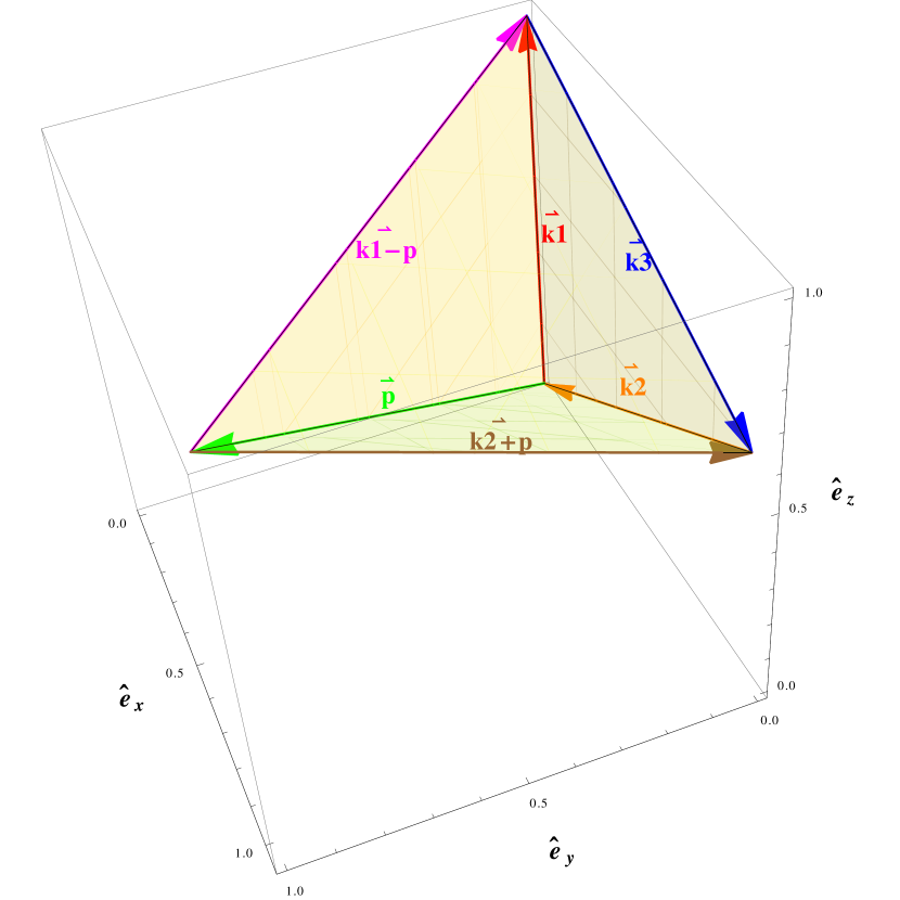
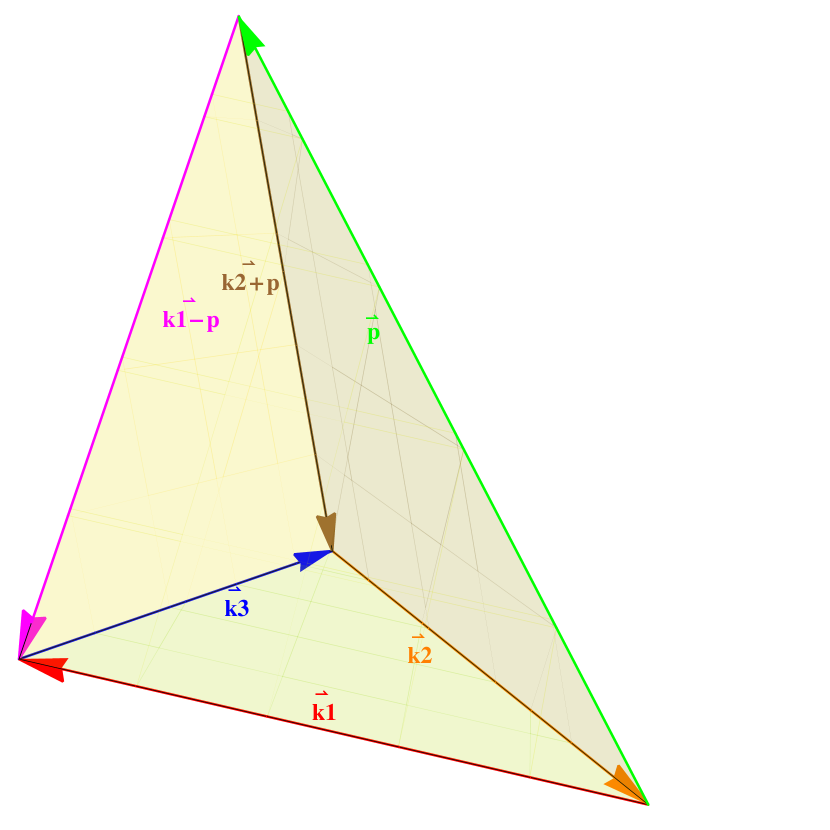
being Fij(𝐤)=Pij(𝐤)PB(𝐤)+iϵijm𝐤^mPH(𝐤)subscript𝐹𝑖𝑗𝐤subscript𝑃𝑖𝑗𝐤subscript𝑃𝐵𝐤𝑖subscriptitalic-ϵ𝑖𝑗𝑚superscript^𝐤𝑚subscript𝑃𝐻𝐤F_{ij}(\mathbf{k})=P_{ij}(\mathbf{k})P_{B}(\mathbf{k})+i\epsilon_{ijm}\hat{\mathbf{k}}^{m}P_{H}(\mathbf{k}). Wavevectors that appear in eq.(3.2) generate a tetrahedron configuration (see figure 1) such that fifteen angles must be included for calculating the bispectrum. So, in order to make comparison with previos works, we use non only the geometry configuration for bispectrum but as well the notation of these angles defined in [65] given as

β=𝐩^𝐤𝟏𝐩^,γ=𝐩^𝐤𝟐+𝐩^,μ=𝐤𝟏𝐩^𝐤𝟐+𝐩^,θkp=𝐤𝟏^𝐤𝟐^formulae-sequence𝛽^𝐩^𝐤𝟏𝐩formulae-sequence𝛾^𝐩^𝐤𝟐𝐩formulae-sequence𝜇^𝐤𝟏𝐩^𝐤𝟐𝐩subscript𝜃𝑘𝑝^𝐤𝟏^𝐤𝟐\displaystyle\beta=\hat{\mathbf{p}}\cdot\widehat{\mathbf{k1}-\mathbf{p}},\quad\gamma=\hat{\mathbf{p}}\cdot\widehat{\mathbf{k2}+\mathbf{p}},\quad\mu=\widehat{\mathbf{k1}-\mathbf{p}}\cdot\widehat{\mathbf{k2}+\mathbf{p}},\quad\theta_{kp}=\hat{\mathbf{k1}}\cdot\hat{\mathbf{k2}} (3.3)
θkq=𝐤𝟏^𝐤𝟑^,θpq=𝐤𝟐^𝐤𝟑^,αk=𝐤𝟏^𝐩^,αp=𝐤𝟐^𝐩^,αq=𝐤𝟑^𝐩^formulae-sequencesubscript𝜃𝑘𝑞^𝐤𝟏^𝐤𝟑formulae-sequencesubscript𝜃𝑝𝑞^𝐤𝟐^𝐤𝟑formulae-sequencesubscript𝛼𝑘^𝐤𝟏^𝐩formulae-sequencesubscript𝛼𝑝^𝐤𝟐^𝐩subscript𝛼𝑞^𝐤𝟑^𝐩\displaystyle\theta_{kq}=\hat{\mathbf{k1}}\cdot\hat{\mathbf{k3}},\quad\theta_{pq}=\hat{\mathbf{k2}}\cdot\hat{\mathbf{k3}},\quad\alpha_{k}=\hat{\mathbf{k1}}\cdot\hat{\mathbf{p}},\quad\alpha_{p}=\hat{\mathbf{k2}}\cdot\hat{\mathbf{p}},\quad\alpha_{q}=\hat{\mathbf{k3}}\cdot\hat{\mathbf{p}}
βk=𝐤𝟏^𝐤𝟏𝐩^,βp=𝐤𝟐^𝐤𝟏𝐩^,,βq=𝐤𝟑^𝐤𝟏𝐩^,γk=𝐤𝟏^𝐤𝟐+𝐩^\displaystyle\beta_{k}=\hat{\mathbf{k1}}\cdot\widehat{\mathbf{k1}-\mathbf{p}},\beta_{p}=\hat{\mathbf{k2}}\cdot\widehat{\mathbf{k1}-\mathbf{p}},\quad,\beta_{q}=\hat{\mathbf{k3}}\cdot\widehat{\mathbf{k1}-\mathbf{p}},\quad\gamma_{k}=\hat{\mathbf{k1}}\cdot\widehat{\mathbf{k2}+\mathbf{p}}
γp=𝐤𝟐^𝐤𝟐+𝐩^,γq=𝐤𝟑^𝐤𝟐+𝐩^.formulae-sequencesubscript𝛾𝑝^𝐤𝟐^𝐤𝟐𝐩subscript𝛾𝑞^𝐤𝟑^𝐤𝟐𝐩\displaystyle\gamma_{p}=\hat{\mathbf{k2}}\cdot\widehat{\mathbf{k2}+\mathbf{p}},\quad\gamma_{q}=\hat{\mathbf{k3}}\cdot\widehat{\mathbf{k2}+\mathbf{p}}.
Refer to caption
Refer to caption
Figure 1: Geometrical configuration for bispectrum. The wavevectors 𝐤𝟏𝐤𝟏\mathbf{k1}, 𝐤𝟐𝐤𝟐\mathbf{k2} and 𝐤𝟑𝐤𝟑\mathbf{k3} are free, while 𝐩𝐩\mathbf{p} is the integration mode.

As we will see, the bispectrum has two main contributions, the first contribution contains terms proportional to AB3superscriptsubscript𝐴𝐵3A_{B}^{3} or ABAH2subscript𝐴𝐵subscriptsuperscript𝐴2𝐻A_{B}A^{2}_{H} and this is called the even contribution denoted here with B(S)superscript𝐵𝑆B^{(S)}. The second contribution is proportional to terms like AH3superscriptsubscript𝐴𝐻3A_{H}^{3} or AB2AHsuperscriptsubscript𝐴𝐵2subscript𝐴𝐻A_{B}^{2}A_{H} and it is called the odd contribution denoted as (A)superscript𝐴\mathcal{B}^{(A)}. Hence, we can define the three-point correlation for the scalar modes as

Z1(𝐤𝟏)Z2(𝐤𝟐)Z3(𝐤𝟑)δ(i=13𝐤𝐢)(BZ1Z2Z3(S)iϵljkZ1Z2Z3(A)ljk),delimited-⟨⟩subscript𝑍1𝐤𝟏subscript𝑍2𝐤𝟐subscript𝑍3𝐤𝟑𝛿superscriptsubscript𝑖13𝐤𝐢superscriptsubscript𝐵subscript𝑍1subscript𝑍2subscript𝑍3𝑆𝑖subscriptitalic-ϵ𝑙𝑗𝑘superscriptsubscriptsubscript𝑍1subscript𝑍2subscript𝑍3𝐴𝑙𝑗𝑘\langle Z_{1}(\mathbf{k1})Z_{2}(\mathbf{k2})Z_{3}(\mathbf{k3})\rangle\equiv\delta\left(\sum_{i=1}^{3}\mathbf{ki}\right)\left(B_{Z_{1}Z_{2}Z_{3}}^{(S)}-i\epsilon_{ljk}\mathcal{B}_{Z_{1}Z_{2}Z_{3}}^{(A\,)\,ljk}\right), (3.4)

where Z{1,2,3}={ρB,ΠB(S)}subscript𝑍123subscript𝜌𝐵subscriptsuperscriptΠ𝑆𝐵Z_{\{1,2,3\}}=\{\rho_{B},\Pi^{(S)}_{B}\}. We begin calculating the bispectrum of the magnetic energy density. To do so, we shall apply the projector defined in eq.(2) three times δijδtlδmnsubscript𝛿𝑖𝑗subscript𝛿𝑡𝑙subscript𝛿𝑚𝑛\delta_{ij}\delta_{tl}\delta_{mn} on eq.( 3.1) to obtain the following

Πij(𝐤𝟏)Πtl(𝐤𝟐)Πmn(𝐤𝟑)δijδtlδmn=ρB(𝐤𝟏)ρB(𝐤𝟐)ρB(𝐤𝟑),delimited-⟨⟩subscriptΠ𝑖𝑗𝐤𝟏subscriptΠ𝑡𝑙𝐤𝟐subscriptΠ𝑚𝑛𝐤𝟑subscript𝛿𝑖𝑗subscript𝛿𝑡𝑙subscript𝛿𝑚𝑛delimited-⟨⟩subscript𝜌𝐵𝐤𝟏subscript𝜌𝐵𝐤𝟐subscript𝜌𝐵𝐤𝟑\langle\Pi_{ij}(\mathbf{k1})\Pi_{tl}(\mathbf{k2})\Pi_{mn}(\mathbf{k3})\rangle\delta_{ij}\delta_{tl}\delta_{mn}=\langle\rho_{B}(\mathbf{k1})\rho_{B}(\mathbf{k2})\rho_{B}(\mathbf{k3})\rangle, (3.5)

using eq.(3.4), a straightforward calculation gives the following expression

BρBρBρB(S)superscriptsubscript𝐵subscript𝜌𝐵subscript𝜌𝐵subscript𝜌𝐵𝑆\displaystyle B_{\rho_{B}\rho_{B}\rho_{B}}^{(S)} =\displaystyle= 8(2π)3(4πργ,0)3d3p(PB(p)PB(|𝐤𝟏𝐩|)PB(|𝐩+𝐤𝟐|)Fρρρ1\displaystyle\frac{8}{(2\pi)^{3}(4\pi\rho_{\gamma,0})^{3}}\int d^{3}p\left(P_{B}(p)P_{B}(\left|\mathbf{k1}-\mathbf{p}\right|)P_{B}(\left|\mathbf{p}+\mathbf{k2}\right|)F_{\rho\rho\rho}^{1}\right. (3.6)
+\displaystyle+ PH(|𝐩+𝐤𝟐|)(PB(p)PH(|𝐤𝟏𝐩|)Fρρρ2+PB(|𝐤𝟏𝐩|)PH(p)Fρρρ3)subscript𝑃𝐻𝐩𝐤𝟐subscript𝑃𝐵𝑝subscript𝑃𝐻𝐤𝟏𝐩superscriptsubscript𝐹𝜌𝜌𝜌2subscript𝑃𝐵𝐤𝟏𝐩subscript𝑃𝐻𝑝superscriptsubscript𝐹𝜌𝜌𝜌3\displaystyle P_{H}(\left|\mathbf{p}+\mathbf{k2}\right|)(-P_{B}(p)P_{H}(\left|\mathbf{k1}-\mathbf{p}\right|)F_{\rho\rho\rho}^{2}+P_{B}(\left|\mathbf{k1}-\mathbf{p}\right|)P_{H}(p)F_{\rho\rho\rho}^{3})
\displaystyle- PB(|𝐩+𝐤𝟐|)PH(p)PH(|𝐤𝟏𝐩|)Fρρρ4),\displaystyle\left.P_{B}(\left|\mathbf{p}+\mathbf{k2}\right|)P_{H}(p)P_{H}(\left|\mathbf{k1}-\mathbf{p}\right|)F_{\rho\rho\rho}^{4}\right),

for the even contribution. The values of Fρρρsubscript𝐹𝜌𝜌𝜌F_{\rho\rho\rho} are shown along with the odd contribution in appendix A. In orden to find the three-point cross-correlation between scalar anisotropic stress and magnetic energy density, we will apply the three projections δijδtl𝒫mnsubscript𝛿𝑖𝑗subscript𝛿𝑡𝑙subscript𝒫𝑚𝑛\delta_{ij}\delta_{tl}\mathcal{P}_{mn} defined in eq.(2) on eq.(3.1) which gives us

Πij(𝐤𝟏)Πtl(𝐤𝟐)Πmn(𝐤𝟑)δijδtl𝒫mn=ρB(𝐤𝟏)ρB(𝐤𝟐)ΠB(S)(𝐤𝟑),delimited-⟨⟩subscriptΠ𝑖𝑗𝐤𝟏subscriptΠ𝑡𝑙𝐤𝟐subscriptΠ𝑚𝑛𝐤𝟑subscript𝛿𝑖𝑗subscript𝛿𝑡𝑙subscript𝒫𝑚𝑛delimited-⟨⟩subscript𝜌𝐵𝐤𝟏subscript𝜌𝐵𝐤𝟐superscriptsubscriptΠ𝐵𝑆𝐤𝟑\langle\Pi_{ij}(\mathbf{k1})\Pi_{tl}(\mathbf{k2})\Pi_{mn}(\mathbf{k3})\rangle\delta_{ij}\delta_{tl}\mathcal{P}_{mn}=\langle\rho_{B}(\mathbf{k1})\rho_{B}(\mathbf{k2})\Pi_{B}^{(S)}(\mathbf{k3})\rangle, (3.7)

and using the three-point correlation eq.(3.4), the even contribution yields

BρBρBΠB(S)(S)superscriptsubscript𝐵subscript𝜌𝐵subscript𝜌𝐵superscriptsubscriptΠ𝐵𝑆𝑆\displaystyle B_{\rho_{B}\rho_{B}\Pi_{B}^{(S)}}^{(S)} =\displaystyle= 82(2π)3(4πργ,0)3d3p(PB(p)PB(|𝐤𝟏𝐩|)PB(|𝐩+𝐤𝟐|)FρρΠ(S)1\displaystyle\frac{8}{2(2\pi)^{3}(4\pi\rho_{\gamma,0})^{3}}\int d^{3}p\left(-P_{B}(p)P_{B}(\left|\mathbf{k1}-\mathbf{p}\right|)P_{B}(\left|\mathbf{p}+\mathbf{k2}\right|)F_{\rho\rho\Pi^{(S)}}^{1}\right. (3.8)
\displaystyle- PB(p)PH(|𝐤𝟏𝐩|)PH(|𝐩+𝐤𝟐|)FρρΠ(S)2subscript𝑃𝐵𝑝subscript𝑃𝐻𝐤𝟏𝐩subscript𝑃𝐻𝐩𝐤𝟐superscriptsubscript𝐹𝜌𝜌superscriptΠ𝑆2\displaystyle P_{B}(p)P_{H}(\left|\mathbf{k1}-\mathbf{p}\right|)P_{H}(\left|\mathbf{p}+\mathbf{k2}\right|)F_{\rho\rho\Pi^{(S)}}^{2}
+\displaystyle+ PH(p)(PH(|𝐩+𝐤𝟐|)PB(|𝐤𝟏𝐩|)FρρΠ(S)3\displaystyle P_{H}(p)\left(-P_{H}(\left|\mathbf{p}+\mathbf{k2}\right|)P_{B}(\left|\mathbf{k1}-\mathbf{p}\right|)F_{\rho\rho\Pi^{(S)}}^{3}\right.
+\displaystyle+ PB(|𝐩+𝐤𝟐|)PH(|𝐤𝟏𝐩|)FρρΠ(S)4)).\displaystyle\left.\left.P_{B}(\left|\mathbf{p}+\mathbf{k2}\right|)P_{H}(\left|\mathbf{k1}-\mathbf{p}\right|)F_{\rho\rho\Pi^{(S)}}^{4}\right)\right).

Other cross-bispectra is obtained by applying δij𝒫tl𝒫mnsubscript𝛿𝑖𝑗subscript𝒫𝑡𝑙subscript𝒫𝑚𝑛\delta_{ij}\mathcal{P}_{tl}\mathcal{P}_{mn} on eq.(3.1) and this gives

Πij(𝐤𝟏)Πtl(𝐤𝟐)Πmn(𝐤𝟑)δij𝒫tl𝒫mn=ρB(𝐤𝟏)ΠB(S)(𝐤𝟐)ΠB(S)(𝐤𝟑),delimited-⟨⟩subscriptΠ𝑖𝑗𝐤𝟏subscriptΠ𝑡𝑙𝐤𝟐subscriptΠ𝑚𝑛𝐤𝟑subscript𝛿𝑖𝑗subscript𝒫𝑡𝑙subscript𝒫𝑚𝑛delimited-⟨⟩subscript𝜌𝐵𝐤𝟏superscriptsubscriptΠ𝐵𝑆𝐤𝟐superscriptsubscriptΠ𝐵𝑆𝐤𝟑\langle\Pi_{ij}(\mathbf{k1})\Pi_{tl}(\mathbf{k2})\Pi_{mn}(\mathbf{k3})\rangle\delta_{ij}\mathcal{P}_{tl}\mathcal{P}_{mn}=\langle\rho_{B}(\mathbf{k1})\Pi_{B}^{(S)}(\mathbf{k2})\Pi_{B}^{(S)}(\mathbf{k3})\rangle, (3.9)

as result we found the following expression

BρBΠB(S)ΠB(S)(S)superscriptsubscript𝐵subscript𝜌𝐵superscriptsubscriptΠ𝐵𝑆superscriptsubscriptΠ𝐵𝑆𝑆\displaystyle B_{\rho_{B}\Pi_{B}^{(S)}\Pi_{B}^{(S)}}^{(S)} =\displaystyle= 84(2π)3(4πργ,0)3d3p(PB(p)PB(|𝐤𝟏𝐩|)PB(|𝐩+𝐤𝟐|)FρΠ(S)Π(S)1\displaystyle\frac{8}{4(2\pi)^{3}(4\pi\rho_{\gamma,0})^{3}}\int d^{3}p\left(P_{B}(p)P_{B}(\left|\mathbf{k1}-\mathbf{p}\right|)P_{B}(\left|\mathbf{p}+\mathbf{k2}\right|)F_{\rho\Pi^{(S)}\Pi^{(S)}}^{1}\right. (3.10)
+\displaystyle+ PB(p)PH(|𝐩+𝐤𝟐|)PH(|𝐤𝟏𝐩|)FρΠ(S)Π(S)2subscript𝑃𝐵𝑝subscript𝑃𝐻𝐩𝐤𝟐subscript𝑃𝐻𝐤𝟏𝐩superscriptsubscript𝐹𝜌superscriptΠ𝑆superscriptΠ𝑆2\displaystyle P_{B}(p)P_{H}(\left|\mathbf{p}+\mathbf{k2}\right|)P_{H}(\left|\mathbf{k1}-\mathbf{p}\right|)F_{\rho\Pi^{(S)}\Pi^{(S)}}^{2}
\displaystyle- PH(p)PH(|𝐩+𝐤𝟐|)PB(|𝐤𝟏𝐩|)FρΠ(S)Π(S)3subscript𝑃𝐻𝑝subscript𝑃𝐻𝐩𝐤𝟐subscript𝑃𝐵𝐤𝟏𝐩superscriptsubscript𝐹𝜌superscriptΠ𝑆superscriptΠ𝑆3\displaystyle P_{H}(p)P_{H}(\left|\mathbf{p}+\mathbf{k2}\right|)P_{B}(\left|\mathbf{k1}-\mathbf{p}\right|)F_{\rho\Pi^{(S)}\Pi^{(S)}}^{3}
\displaystyle- PH(p)PH(|𝐤𝟏𝐩|)PB(|𝐩+𝐤𝟐|)FρΠ(S)Π(S)4).\displaystyle\left.P_{H}(p)P_{H}(\left|\mathbf{k1}-\mathbf{p}\right|)P_{B}(\left|\mathbf{p}+\mathbf{k2}\right|)F_{\rho\Pi^{(S)}\Pi^{(S)}}^{4}\right).

Finally the three-point correlation of scalar anisotropic stress is obtained by applying 𝒫ij𝒫tl𝒫mnsubscript𝒫𝑖𝑗subscript𝒫𝑡𝑙subscript𝒫𝑚𝑛\mathcal{P}_{ij}\mathcal{P}_{tl}\mathcal{P}_{mn} on eq.(3.1) finding that

Πij(𝐤𝟏)Πtl(𝐤𝟐)Πmn(𝐤𝟑)𝒫ij𝒫tl𝒫mn=ΠB(S)(𝐤𝟏)ΠB(S)(𝐤𝟐)ΠB(S)(𝐤𝟑),delimited-⟨⟩subscriptΠ𝑖𝑗𝐤𝟏subscriptΠ𝑡𝑙𝐤𝟐subscriptΠ𝑚𝑛𝐤𝟑subscript𝒫𝑖𝑗subscript𝒫𝑡𝑙subscript𝒫𝑚𝑛delimited-⟨⟩superscriptsubscriptΠ𝐵𝑆𝐤𝟏superscriptsubscriptΠ𝐵𝑆𝐤𝟐superscriptsubscriptΠ𝐵𝑆𝐤𝟑\langle\Pi_{ij}(\mathbf{k1})\Pi_{tl}(\mathbf{k2})\Pi_{mn}(\mathbf{k3})\rangle\mathcal{P}_{ij}\mathcal{P}_{tl}\mathcal{P}_{mn}=\langle\Pi_{B}^{(S)}(\mathbf{k1})\Pi_{B}^{(S)}(\mathbf{k2})\Pi_{B}^{(S)}(\mathbf{k3})\rangle, (3.11)

thus, the expression for the bispectrum for that contribution is

BΠB(S)ΠB(S)ΠB(S)(S)superscriptsubscript𝐵superscriptsubscriptΠ𝐵𝑆superscriptsubscriptΠ𝐵𝑆superscriptsubscriptΠ𝐵𝑆𝑆\displaystyle B_{\Pi_{B}^{(S)}\Pi_{B}^{(S)}\Pi_{B}^{(S)}}^{(S)} =\displaystyle= 1(2π)3(4πργ,0)3d3p(PB(p)PB(|𝐤𝟏𝐩|)PB(|𝐩+𝐤𝟐|)FΠ(S)Π(S)Π(S)1\displaystyle\frac{1}{(2\pi)^{3}(4\pi\rho_{\gamma,0})^{3}}\int d^{3}p\left(-P_{B}(p)P_{B}(\left|\mathbf{k1}-\mathbf{p}\right|)P_{B}(\left|\mathbf{p}+\mathbf{k2}\right|)F_{\Pi^{(S)}\Pi^{(S)}\Pi^{(S)}}^{1}\right. (3.12)
\displaystyle- PB(p)PH(|𝐩+𝐤𝟐|)PH(|𝐤𝟏𝐩|)FΠ(S)Π(S)Π(S)2subscript𝑃𝐵𝑝subscript𝑃𝐻𝐩𝐤𝟐subscript𝑃𝐻𝐤𝟏𝐩superscriptsubscript𝐹superscriptΠ𝑆superscriptΠ𝑆superscriptΠ𝑆2\displaystyle P_{B}(p)P_{H}(\left|\mathbf{p}+\mathbf{k2}\right|)P_{H}(\left|\mathbf{k1}-\mathbf{p}\right|)F_{\Pi^{(S)}\Pi^{(S)}\Pi^{(S)}}^{2}
+\displaystyle+ PH(p)PB(|𝐩+𝐤𝟐|)PH(|𝐤𝟏𝐩|)FΠ(S)Π(S)Π(S)3subscript𝑃𝐻𝑝subscript𝑃𝐵𝐩𝐤𝟐subscript𝑃𝐻𝐤𝟏𝐩superscriptsubscript𝐹superscriptΠ𝑆superscriptΠ𝑆superscriptΠ𝑆3\displaystyle P_{H}(p)P_{B}(\left|\mathbf{p}+\mathbf{k2}\right|)P_{H}(\left|\mathbf{k1}-\mathbf{p}\right|)F_{\Pi^{(S)}\Pi^{(S)}\Pi^{(S)}}^{3}
+\displaystyle+ PH(p)PB(|𝐤𝟏𝐩|)PH(|𝐩+𝐤𝟐|)FΠ(S)Π(S)Π(S)4).\displaystyle\left.P_{H}(p)P_{B}(\left|\mathbf{k1}-\mathbf{p}\right|)P_{H}(\left|\mathbf{p}+\mathbf{k2}\right|)F_{\Pi^{(S)}\Pi^{(S)}\Pi^{(S)}}^{4}\right).

Again, the FΠΠΠsubscript𝐹ΠΠΠF_{\Pi\Pi\Pi}’s values can be checked along with the odd contribution in appendix A. In the case where the helicity of the field is not considered (AH=0)subscript𝐴𝐻0(A_{H}=0), the only contribution that remains is sourced from AB3subscriptsuperscript𝐴3𝐵A^{3}_{B}. The results of this contribution were reported in [65] and we have found the same expressions. Therefore, we have generalized those previous results to even and odd contributions of the PMFs bispectrum and thus these findings are the first results of the paper.

4 Full Evaluation

With the derivation of the angular part of the three-point correlation for each component of the magnetic tensor, we proceed to make the evaluation of the above integrals. Due to the complexity of the calculation, we are going to follow the exact methodology proposed in [48, 49, 50]. They consider two cases for finding solution of the correlator. In the first case, the terms dependent on the integration vector 𝐩𝐩\mathbf{p} are not considered in the evaluation. For the second case, the squeezed collinear configuration is used to make predictions. We will use five representative shapes of the bispectrum which are shown in the Figure 2. The odd signal arising from (A)superscript𝐴\mathcal{B}^{(A\,)} will not be considered here but will be deferred for later work.

Refer to caption
Figure 2: Geometrical representations for the bispectrum. The figure shows a visual representation of the triangles and the collinear configuration of the bispectrum shape. The table in the bottom-right panel describes the values of the 𝐩𝐩\mathbf{p}-independent terms for each configuration.

4.1 𝐩𝐩\mathbf{p}-independent

For this case, the only terms which appear in the evaluation are those angles given in eq.(3.3) independent of 𝐩𝐩\mathbf{p}; they are (θkpsubscript𝜃𝑘𝑝\theta_{kp}, θkqsubscript𝜃𝑘𝑞\theta_{kq}, θpqsubscript𝜃𝑝𝑞\theta_{pq}). The values of these angles for each configuration are shown in figure 2. The F𝐹F’s functions defined above take the following values under this approximation

Fρρρ1=μ2,Fρρρ2=μ,Fρρρ3=Fρρρ4=0,formulae-sequencesuperscriptsubscript𝐹𝜌𝜌𝜌1superscript𝜇2formulae-sequencesuperscriptsubscript𝐹𝜌𝜌𝜌2𝜇superscriptsubscript𝐹𝜌𝜌𝜌3superscriptsubscript𝐹𝜌𝜌𝜌40F_{\rho\rho\rho}^{1}=\mu^{2},\quad F_{\rho\rho\rho}^{2}=\mu,\quad F_{\rho\rho\rho}^{3}=F_{\rho\rho\rho}^{4}=0, (4.1)
FρρΠ1=μ23,FρρΠ2=μ,FρρΠ3=FρρΠ4=0,formulae-sequencesuperscriptsubscript𝐹𝜌𝜌Π1superscript𝜇23formulae-sequencesuperscriptsubscript𝐹𝜌𝜌Π2𝜇superscriptsubscript𝐹𝜌𝜌Π3superscriptsubscript𝐹𝜌𝜌Π40F_{\rho\rho\Pi}^{1}=\mu^{2}-3,\quad F_{\rho\rho\Pi}^{2}=-\mu,\quad F_{\rho\rho\Pi}^{3}=F_{\rho\rho\Pi}^{4}=0, (4.2)
FρΠΠ1=μ26+9θpq2,FρΠΠ2=(7+9θpq2)μ,FρΠΠ3=FρΠΠ4=0,formulae-sequencesuperscriptsubscript𝐹𝜌ΠΠ1superscript𝜇269superscriptsubscript𝜃𝑝𝑞2formulae-sequencesuperscriptsubscript𝐹𝜌ΠΠ279superscriptsubscript𝜃𝑝𝑞2𝜇superscriptsubscript𝐹𝜌ΠΠ3superscriptsubscript𝐹𝜌ΠΠ40F_{\rho\Pi\Pi}^{1}=\mu^{2}-6+9\theta_{pq}^{2},\quad F_{\rho\Pi\Pi}^{2}=(-7+9\theta_{pq}^{2})\mu,\quad F_{\rho\Pi\Pi}^{3}=F_{\rho\Pi\Pi}^{4}=0, (4.3)
FΠΠΠ1superscriptsubscript𝐹ΠΠΠ1\displaystyle F_{\Pi\Pi\Pi}^{1} =\displaystyle= 9+9θkp227θkpθkqθpq+9θpq2+μ2+9θkq2,FΠΠΠ3=0,99superscriptsubscript𝜃𝑘𝑝227subscript𝜃𝑘𝑝subscript𝜃𝑘𝑞subscript𝜃𝑝𝑞9superscriptsubscript𝜃𝑝𝑞2superscript𝜇29superscriptsubscript𝜃𝑘𝑞2superscriptsubscript𝐹ΠΠΠ30\displaystyle-9+9\theta_{kp}^{2}-27\theta_{kp}\theta_{kq}\theta_{pq}+9\theta_{pq}^{2}+\mu^{2}+9\theta_{kq}^{2},\quad F_{\Pi\Pi\Pi}^{3}=0,
FΠΠΠ2superscriptsubscript𝐹ΠΠΠ2\displaystyle F_{\Pi\Pi\Pi}^{2} =\displaystyle= (13+18θkp2+9θkq227θkpθkqθpq+9θpq2)μ,FΠΠΠ4=0,1318superscriptsubscript𝜃𝑘𝑝29superscriptsubscript𝜃𝑘𝑞227subscript𝜃𝑘𝑝subscript𝜃𝑘𝑞subscript𝜃𝑝𝑞9superscriptsubscript𝜃𝑝𝑞2𝜇superscriptsubscript𝐹ΠΠΠ40\displaystyle(-13+18\theta_{kp}^{2}+9\theta_{kq}^{2}-27\theta_{kp}\theta_{kq}\theta_{pq}+9\theta_{pq}^{2})\mu,\quad F_{\Pi\Pi\Pi}^{4}=0, (4.4)

where the result given for FΠΠΠ1superscriptsubscript𝐹ΠΠΠ1F_{\Pi\Pi\Pi}^{1} is in agreement with the reported in [48]333There is a difference with a minus sign because we are taking a different signature in the metric.. The values of F𝐹F for each geometrical representation of the bispectrum are shown in table 1 and μ=0𝜇0\mu=0 for all configuration except to squeezed configuration where it takes μ1similar-to𝜇1\mu\sim-1.

Configuration Fρρρ1superscriptsubscript𝐹𝜌𝜌𝜌1F_{\rho\rho\rho}^{1} Fρρρ2superscriptsubscript𝐹𝜌𝜌𝜌2F_{\rho\rho\rho}^{2} FρρΠ1superscriptsubscript𝐹𝜌𝜌Π1F_{\rho\rho\Pi}^{1} FρρΠ2superscriptsubscript𝐹𝜌𝜌Π2F_{\rho\rho\Pi}^{2} FρΠΠ1superscriptsubscript𝐹𝜌ΠΠ1F_{\rho\Pi\Pi}^{1} FρΠΠ2superscriptsubscript𝐹𝜌ΠΠ2F_{\rho\Pi\Pi}^{2} FΠΠΠ1superscriptsubscript𝐹ΠΠΠ1F_{\Pi\Pi\Pi}^{1} FΠΠΠ2superscriptsubscript𝐹ΠΠΠ2F_{\Pi\Pi\Pi}^{2}
Squeezed triangle 0 0 -3 0 -6 0 0 0
Equilateral triangle 0 0 -3 0 -15/4 0 -45/8 0
Folded triangle 0 0 -3 0 3 0 -9 0
Squeezed collinear 1 -1 -2 1 4 -2 -8 4
Flattened 0 0 -3 0 3 0 -9 0
Table 1: Values of F𝐹F for different geometrical configurations in the 𝐩𝐩\mathbf{p}-independent case.

4.2 Squeezed Collinear Configuration

n this approximation, the magnitude of one wave vector (𝐤𝟑^^𝐤𝟑\hat{\mathbf{k3}}) is small while the others have equal magnitudes but have opposing directions (𝐤𝟏^=𝐤𝟐^^𝐤𝟏^𝐤𝟐\hat{\mathbf{k1}}=-\hat{\mathbf{k2}}) as shown in figure 2. With this assumption the angles can be reduced to

β𝛽\displaystyle\beta =\displaystyle= 𝐩^𝐤𝟏𝐩^𝐩^𝐤𝟏𝐩^γ,μ𝐤𝟏𝐩^𝐤𝟏𝐩^1,formulae-sequencesimilar-to^𝐩^𝐤𝟏𝐩^𝐩^𝐤𝟏𝐩similar-to𝛾similar-to𝜇^𝐤𝟏𝐩^𝐤𝟏𝐩similar-to1\displaystyle\hat{\mathbf{p}}\cdot\widehat{\mathbf{k1}-\mathbf{p}}\sim-\hat{\mathbf{p}}\cdot\widehat{\mathbf{k1}-\mathbf{p}}\sim-\gamma,\quad\mu\sim-\widehat{\mathbf{k1}-\mathbf{p}}\cdot\widehat{\mathbf{k1}-\mathbf{p}}\sim-1,
αksubscript𝛼𝑘\displaystyle\alpha_{k} similar-to\displaystyle\sim αpαq,βkβpβqγkγpγq.formulae-sequencesimilar-tosubscript𝛼𝑝subscript𝛼𝑞similar-tosubscript𝛽𝑘subscript𝛽𝑝similar-tosubscript𝛽𝑞similar-tosubscript𝛾𝑘similar-tosubscript𝛾𝑝similar-tosubscript𝛾𝑞\displaystyle-\alpha_{p}\sim\alpha_{q},\quad\beta_{k}\sim-\beta_{p}\sim\beta_{q}\sim-\gamma_{k}\sim\gamma_{p}\sim-\gamma_{q}. (4.5)

By using this approximation the values of the F𝐹F’s are simplified to

Fρρρ1=1+β2,Fρρρ2=(1+β2),Fρρρ3=2β,Fρρρ4=2β,formulae-sequencesuperscriptsubscript𝐹𝜌𝜌𝜌11superscript𝛽2formulae-sequencesuperscriptsubscript𝐹𝜌𝜌𝜌21superscript𝛽2formulae-sequencesuperscriptsubscript𝐹𝜌𝜌𝜌32𝛽superscriptsubscript𝐹𝜌𝜌𝜌42𝛽F_{\rho\rho\rho}^{1}=1+\beta^{2},\quad F_{\rho\rho\rho}^{2}=-(1+\beta^{2}),\quad F_{\rho\rho\rho}^{3}=-2\beta,\quad F_{\rho\rho\rho}^{4}=2\beta, (4.6)
FρρΠ1superscriptsubscript𝐹𝜌𝜌Π1\displaystyle F_{\rho\rho\Pi}^{1} =\displaystyle= 2+3αk2+β26αkββk+3βk2+3β2βk2,FρρΠ2=13αk22β2+6αkββk,23superscriptsubscript𝛼𝑘2superscript𝛽26subscript𝛼𝑘𝛽subscript𝛽𝑘3superscriptsubscript𝛽𝑘23superscript𝛽2superscriptsubscript𝛽𝑘2superscriptsubscript𝐹𝜌𝜌Π213superscriptsubscript𝛼𝑘22superscript𝛽26subscript𝛼𝑘𝛽subscript𝛽𝑘\displaystyle-2+3\alpha_{k}^{2}+\beta^{2}-6\alpha_{k}\beta\beta_{k}+3\beta_{k}^{2}+3\beta^{2}\beta_{k}^{2},\quad F_{\rho\rho\Pi}^{2}=1-3\alpha_{k}^{2}-2\beta^{2}+6\alpha_{k}\beta\beta_{k},
FρρΠ3superscriptsubscript𝐹𝜌𝜌Π3\displaystyle F_{\rho\rho\Pi}^{3} =\displaystyle= β(1+3βk2),FρρΠ4=β(1+3βk2),𝛽13superscriptsubscript𝛽𝑘2superscriptsubscript𝐹𝜌𝜌Π4𝛽13superscriptsubscript𝛽𝑘2\displaystyle-\beta(-1+3\beta_{k}^{2}),\quad F_{\rho\rho\Pi}^{4}=\beta(-1+3\beta_{k}^{2}), (4.7)
FρΠΠ1superscriptsubscript𝐹𝜌ΠΠ1\displaystyle F_{\rho\Pi\Pi}^{1} =\displaystyle= 9αkββk3+(23βk2)2+β2(1+3βk2)+αk2(3+9βk2),FρΠΠ3=3αkβkβ(43βk2),9subscript𝛼𝑘𝛽superscriptsubscript𝛽𝑘3superscript23superscriptsubscript𝛽𝑘22superscript𝛽213superscriptsubscript𝛽𝑘2superscriptsubscript𝛼𝑘239superscriptsubscript𝛽𝑘2superscriptsubscript𝐹𝜌ΠΠ33subscript𝛼𝑘subscript𝛽𝑘𝛽43superscriptsubscript𝛽𝑘2\displaystyle-9\alpha_{k}\beta\beta_{k}^{3}+(2-3\beta_{k}^{2})^{2}+\beta^{2}(1+3\beta_{k}^{2})+\alpha_{k}^{2}(-3+9\beta_{k}^{2}),\quad F_{\rho\Pi\Pi}^{3}=3\alpha_{k}\beta_{k}-\beta(4-3\beta_{k}^{2}),
FρΠΠ2superscriptsubscript𝐹𝜌ΠΠ2\displaystyle F_{\rho\Pi\Pi}^{2} =\displaystyle= 22β2+3αkββk+3βk2,FρΠΠ4=6αkβk+9αkβk3β(5+6βk2),22superscript𝛽23subscript𝛼𝑘𝛽subscript𝛽𝑘3superscriptsubscript𝛽𝑘2superscriptsubscript𝐹𝜌ΠΠ46subscript𝛼𝑘subscript𝛽𝑘9subscript𝛼𝑘superscriptsubscript𝛽𝑘3𝛽56superscriptsubscript𝛽𝑘2\displaystyle-2-2\beta^{2}+3\alpha_{k}\beta\beta_{k}+3\beta_{k}^{2},\quad F_{\rho\Pi\Pi}^{4}=-6\alpha_{k}\beta_{k}+9\alpha_{k}\beta_{k}^{3}-\beta(-5+6\beta_{k}^{2}), (4.8)
FΠΠΠ1superscriptsubscript𝐹ΠΠΠ1\displaystyle F_{\Pi\Pi\Pi}^{1} =\displaystyle= 8+β2+18βk2+3β2βk29βk4+6αkββk(13βk2)+9αk2(13βk2+3βk4),8superscript𝛽218superscriptsubscript𝛽𝑘23superscript𝛽2superscriptsubscript𝛽𝑘29superscriptsubscript𝛽𝑘46subscript𝛼𝑘𝛽subscript𝛽𝑘13superscriptsubscript𝛽𝑘29superscriptsubscript𝛼𝑘213superscriptsubscript𝛽𝑘23superscriptsubscript𝛽𝑘4\displaystyle-8+\beta^{2}+18\beta_{k}^{2}+3\beta^{2}\beta_{k}^{2}-9\beta_{k}^{4}+6\alpha_{k}\beta\beta_{k}(1-3\beta_{k}^{2})+9\alpha_{k}^{2}(1-3\beta_{k}^{2}+3\beta_{k}^{4}),
FΠΠΠ2superscriptsubscript𝐹ΠΠΠ2\displaystyle F_{\Pi\Pi\Pi}^{2} =\displaystyle= 42β23βk2+αk2(6+9βk2),FΠΠΠ3=FΠΠΠ4=(2β3αkβk)(13βk2).42superscript𝛽23superscriptsubscript𝛽𝑘2superscriptsubscript𝛼𝑘269superscriptsubscript𝛽𝑘2superscriptsubscript𝐹ΠΠΠ3superscriptsubscript𝐹ΠΠΠ42𝛽3subscript𝛼𝑘subscript𝛽𝑘13superscriptsubscript𝛽𝑘2\displaystyle 4-2\beta^{2}-3\beta_{k}^{2}+\alpha_{k}^{2}(-6+9\beta_{k}^{2}),\quad F_{\Pi\Pi\Pi}^{3}=F_{\Pi\Pi\Pi}^{4}=(2\beta-3\alpha_{k}\beta_{k})(1-3\beta_{k}^{2}). (4.9)

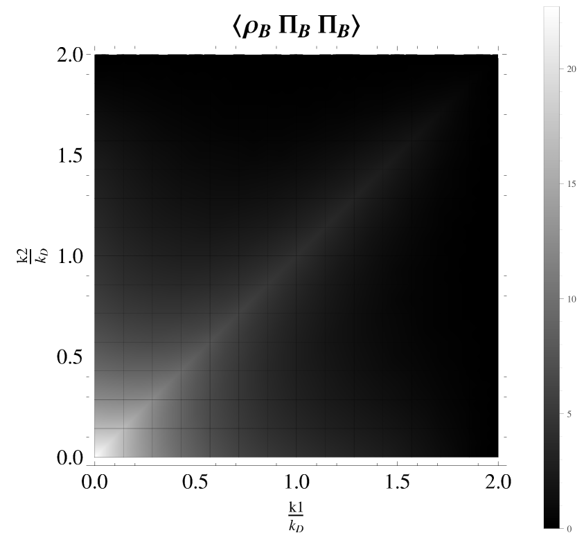
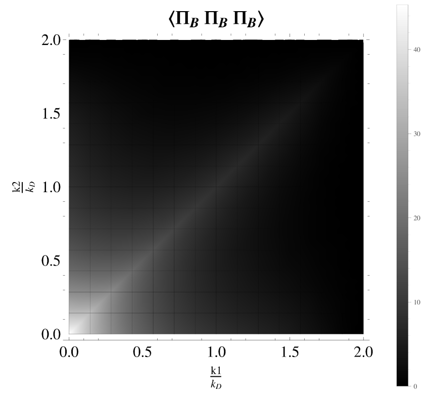
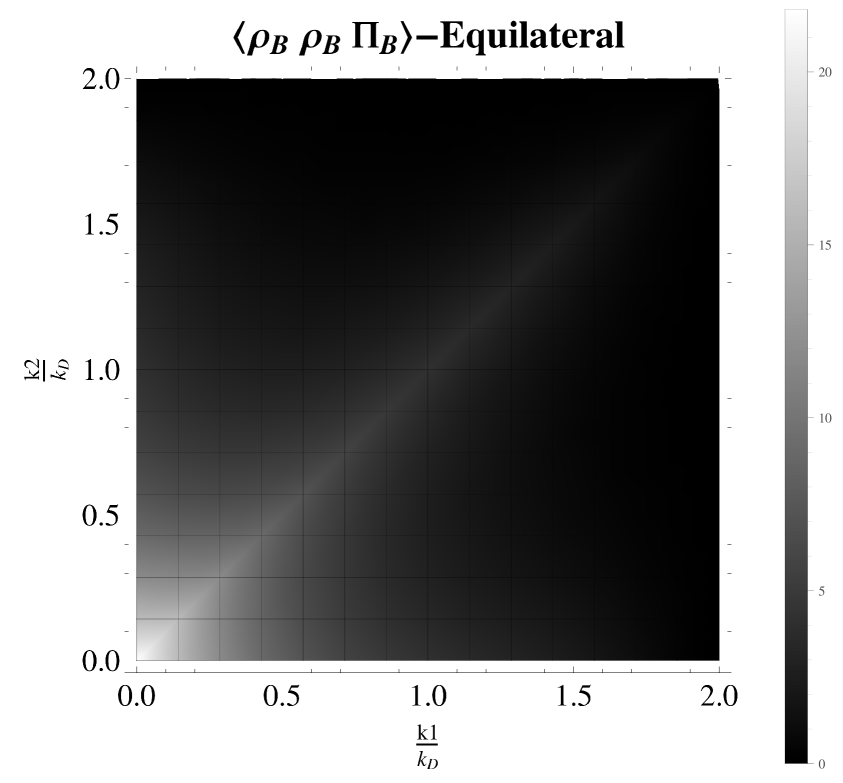
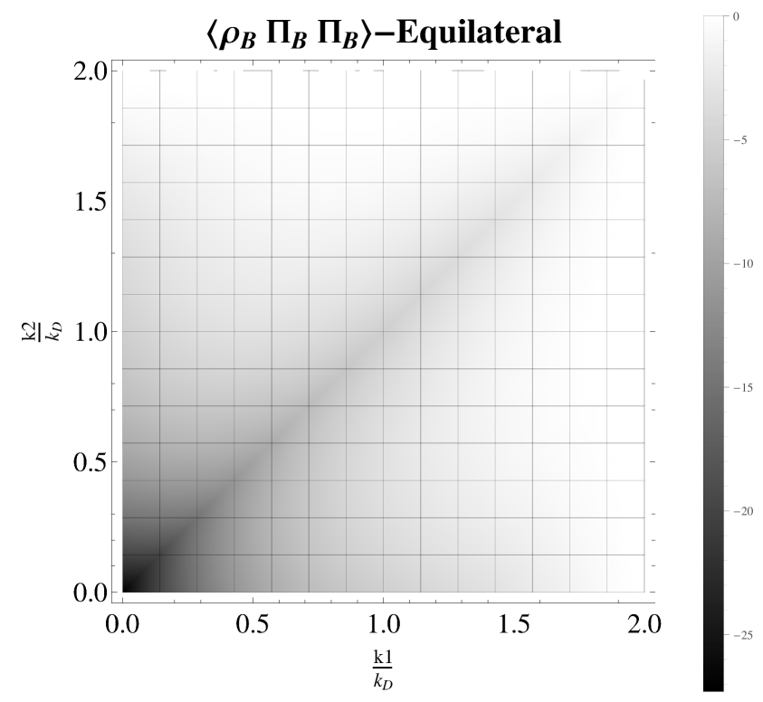
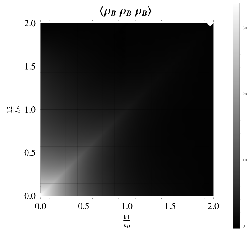
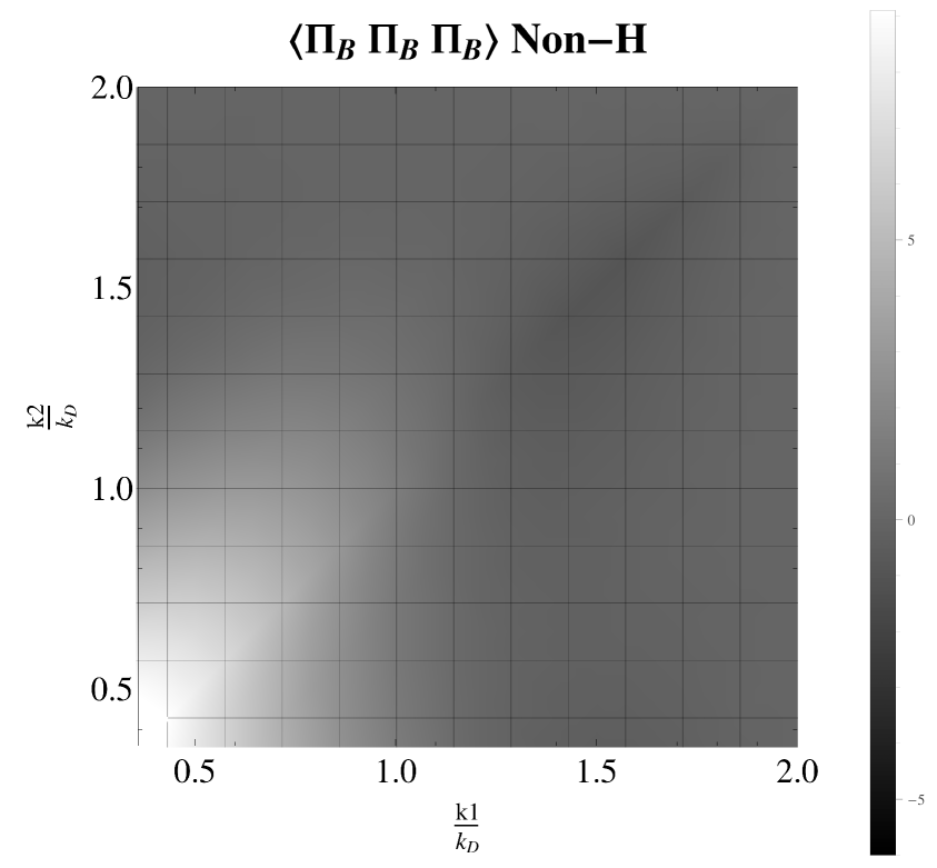
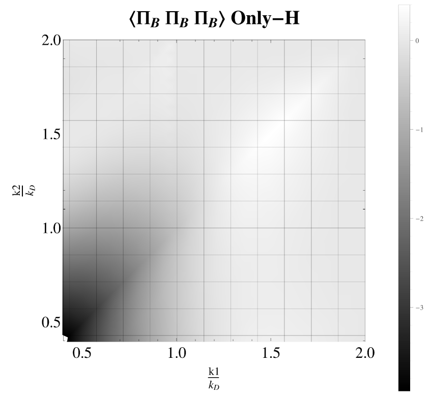
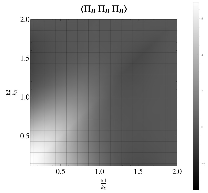
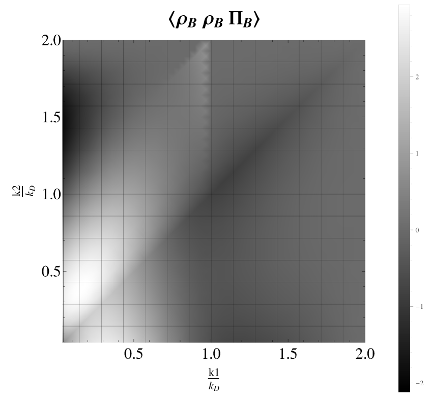
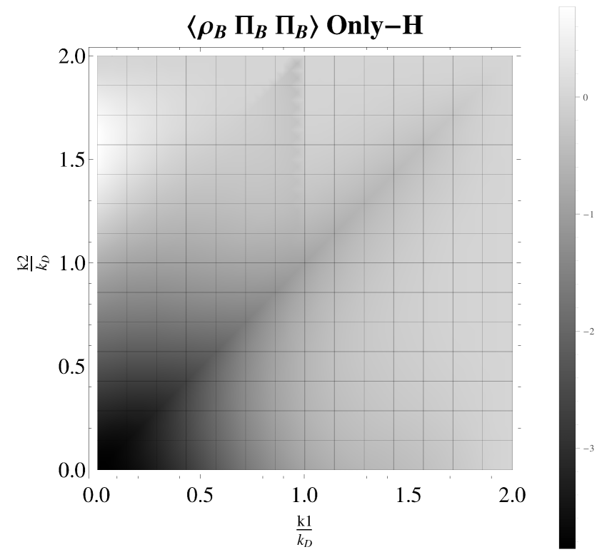
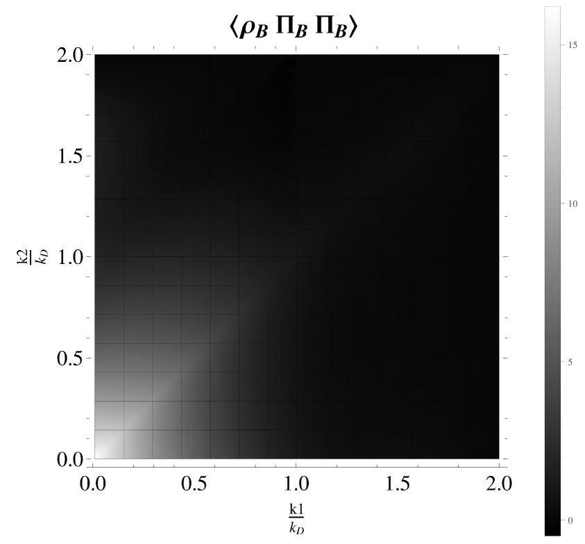
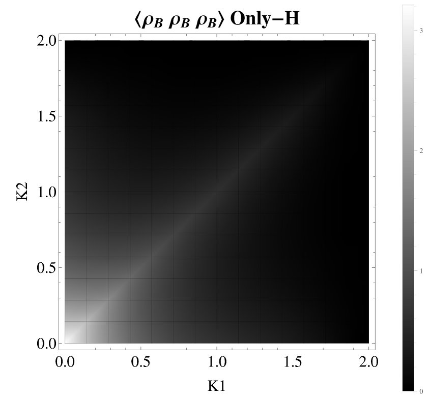
Same results have been obtained in [48] for FΠΠΠ1superscriptsubscript𝐹ΠΠΠ1F_{\Pi\Pi\Pi}^{1} (case where there is not helicity). The angular part of the integrals must be written in spherical coordinates d3p=p2dpdαkdθsuperscript𝑑3𝑝superscript𝑝2𝑑𝑝𝑑subscript𝛼𝑘𝑑𝜃d^{3}p=p^{2}dpd\alpha_{k}d\theta, where θ𝜃\theta is the azimuthal angle. Since we consider an upper cut-off kDsubscript𝑘𝐷k_{D}, we must introduce the (k1,k2𝑘1𝑘2k1,k2)-dependence on the angular integration domain; this implies that we should split the integral domain in different regions such as 0<k1,k2<2kDformulae-sequence0𝑘1𝑘22subscript𝑘𝐷0<k1,k2<2k_{D}. The integration domains we use for calculating the integrals are shown in appendix B. By using the power spectrum expression for the magnetic fields eqs.(2.5)-(2.6) and the F’s values for the 𝐩limit-from𝐩\mathbf{p}-independent case given above, we get the causal magnetic bispectrum (nB=nH=2subscript𝑛𝐵subscript𝑛𝐻2n_{B}=n_{H}=2) which is shown in the Figure 3. We see that the most contribution for the bispectrum occurs when k1k2similar-to𝑘1𝑘2k1\sim k2 and ΠBΠBΠBdelimited-⟨⟩subscriptΠ𝐵subscriptΠ𝐵subscriptΠ𝐵\langle\Pi_{B}\Pi_{B}\Pi_{B}\rangle generates the largest value for scalar mode. Hence, we conclude that the shape of the non-Gaussian associated with the PMF can be classified into the local-type configuration as was previously reported in [51] for a scale invariant shape. We also observe that effects from ABAH2subscript𝐴𝐵superscriptsubscript𝐴𝐻2A_{B}A_{H}^{2} contribution are smaller with respect to AB3superscriptsubscript𝐴𝐵3A_{B}^{3}. The figures 3(g), 3(h) show the cross-correlation of the bispectrum obtaining the same behavior and a large contribution (with respect to the energy density bispectrum).

Refer to caption
(a) Three-point correlation of ρBρBρBdelimited-⟨⟩subscript𝜌𝐵subscript𝜌𝐵subscript𝜌𝐵\langle\rho_{B}\rho_{B}\rho_{B}\rangle in units of 8(2π)3(4πργ,0)38superscript2𝜋3superscript4𝜋subscript𝜌𝛾03\frac{8}{(2\pi)^{3}(4\pi\rho_{\gamma,0})^{3}} only for AB3superscriptsubscript𝐴𝐵3A_{B}^{3}.
Refer to caption
(b) Three-point correlation of ρBρBρBdelimited-⟨⟩subscript𝜌𝐵subscript𝜌𝐵subscript𝜌𝐵\langle\rho_{B}\rho_{B}\rho_{B}\rangle in units of 8(2π)3(4πργ,0)38superscript2𝜋3superscript4𝜋subscript𝜌𝛾03\frac{8}{(2\pi)^{3}(4\pi\rho_{\gamma,0})^{3}} only with ABAH2subscript𝐴𝐵superscriptsubscript𝐴𝐻2A_{B}A_{H}^{2}.
Refer to caption
(c) Even contribution of three-point correlation of ρBρBρBdelimited-⟨⟩subscript𝜌𝐵subscript𝜌𝐵subscript𝜌𝐵\langle\rho_{B}\rho_{B}\rho_{B}\rangle in units of 8(2π)3(4πργ,0)38superscript2𝜋3superscript4𝜋subscript𝜌𝛾03\frac{8}{(2\pi)^{3}(4\pi\rho_{\gamma,0})^{3}}.
Refer to caption
(d) Even contribution of three-point correlation of ρBρBΠBdelimited-⟨⟩subscript𝜌𝐵subscript𝜌𝐵subscriptΠ𝐵\langle\rho_{B}\rho_{B}\Pi_{B}\rangle in units of 4(2π)3(4πργ,0)34superscript2𝜋3superscript4𝜋subscript𝜌𝛾03\frac{4}{(2\pi)^{3}(4\pi\rho_{\gamma,0})^{3}}.
Refer to caption
(e) Even contribution of three-point correlation of ρBΠBΠBdelimited-⟨⟩subscript𝜌𝐵subscriptΠ𝐵subscriptΠ𝐵\langle\rho_{B}\Pi_{B}\Pi_{B}\rangle in units of 2(2π)3(4πργ,0)32superscript2𝜋3superscript4𝜋subscript𝜌𝛾03\frac{2}{(2\pi)^{3}(4\pi\rho_{\gamma,0})^{3}}.
Refer to caption
(f) Even contribution of three-point correlation of ΠBΠBΠBdelimited-⟨⟩subscriptΠ𝐵subscriptΠ𝐵subscriptΠ𝐵\langle\Pi_{B}\Pi_{B}\Pi_{B}\rangle in units of 1(2π)3(4πργ,0)31superscript2𝜋3superscript4𝜋subscript𝜌𝛾03\frac{1}{(2\pi)^{3}(4\pi\rho_{\gamma,0})^{3}}.
Refer to caption
(g) Even contribution of three-point correlation of ρBρBΠBdelimited-⟨⟩subscript𝜌𝐵subscript𝜌𝐵subscriptΠ𝐵\langle\rho_{B}\rho_{B}\Pi_{B}\rangle in units of 4(2π)3(4πργ,0)34superscript2𝜋3superscript4𝜋subscript𝜌𝛾03\frac{4}{(2\pi)^{3}(4\pi\rho_{\gamma,0})^{3}} in the equilateral configuration.
Refer to caption
(h) Even contribution of three-point correlation of ρBΠBΠBdelimited-⟨⟩subscript𝜌𝐵subscriptΠ𝐵subscriptΠ𝐵\langle\rho_{B}\Pi_{B}\Pi_{B}\rangle in units of 2(2π)3(4πργ,0)32superscript2𝜋3superscript4𝜋subscript𝜌𝛾03\frac{2}{(2\pi)^{3}(4\pi\rho_{\gamma,0})^{3}} in the equilateral configuration.
Refer to caption
(i) Even contribution of three-point correlation of ΠBΠBΠBdelimited-⟨⟩subscriptΠ𝐵subscriptΠ𝐵subscriptΠ𝐵\langle\Pi_{B}\Pi_{B}\Pi_{B}\rangle in units of 1(2π)3(4πργ,0)31superscript2𝜋3superscript4𝜋subscript𝜌𝛾03\frac{1}{(2\pi)^{3}(4\pi\rho_{\gamma,0})^{3}} in the equilateral configuration.
Figure 3: Total contribution of three-point correlation of all scalar modes described in the text using the p-independent approximation. The figures (a), (b) (c) show the three-point correlation of the energy density of the magnetic field without, with ABAH2subscript𝐴𝐵superscriptsubscript𝐴𝐻2A_{B}A_{H}^{2} and full contribution respectively. The figures (d), (e) and (f) show the cross three-point correlation of the field. Finally, the figures (g), (h) (i) show the cross three-point correlation field in the equilateral configuration, where the ρBΠBΠBdelimited-⟨⟩subscript𝜌𝐵subscriptΠ𝐵subscriptΠ𝐵\langle\rho_{B}\Pi_{B}\Pi_{B}\rangle has a total negative contribution. We can see that largest contribution to the bispectrum is obtained when k1k2similar-to𝑘1𝑘2k1\sim k2. We can also see that biggest contributions to the scalar modes is given by ΠBΠBΠBdelimited-⟨⟩subscriptΠ𝐵subscriptΠ𝐵subscriptΠ𝐵\langle\Pi_{B}\Pi_{B}\Pi_{B}\rangle when we consider a squeezed configuration.
Refer to caption
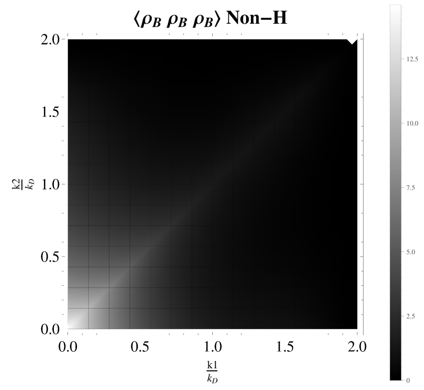
(a) Three-point correlation of ρBρBρBdelimited-⟨⟩subscript𝜌𝐵subscript𝜌𝐵subscript𝜌𝐵\langle\rho_{B}\rho_{B}\rho_{B}\rangle in units of 8(2π)3(4πργ,0)38superscript2𝜋3superscript4𝜋subscript𝜌𝛾03\frac{8}{(2\pi)^{3}(4\pi\rho_{\gamma,0})^{3}} without ABAH2subscript𝐴𝐵superscriptsubscript𝐴𝐻2A_{B}A_{H}^{2}.
Refer to caption
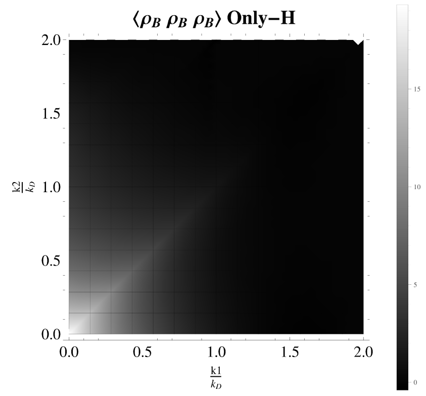
(b) Three-point correlation of ρBρBρBdelimited-⟨⟩subscript𝜌𝐵subscript𝜌𝐵subscript𝜌𝐵\langle\rho_{B}\rho_{B}\rho_{B}\rangle in units of 8(2π)3(4πργ,0)38superscript2𝜋3superscript4𝜋subscript𝜌𝛾03\frac{8}{(2\pi)^{3}(4\pi\rho_{\gamma,0})^{3}} only with ABAH2subscript𝐴𝐵superscriptsubscript𝐴𝐻2A_{B}A_{H}^{2}.
Refer to caption
(c) Even contribution of three-point correlation of ρBρBρBdelimited-⟨⟩subscript𝜌𝐵subscript𝜌𝐵subscript𝜌𝐵\langle\rho_{B}\rho_{B}\rho_{B}\rangle in units of 8(2π)3(4πργ,0)38superscript2𝜋3superscript4𝜋subscript𝜌𝛾03\frac{8}{(2\pi)^{3}(4\pi\rho_{\gamma,0})^{3}}.
Refer to caption
(d) Three-point correlation of ΠBΠBΠBdelimited-⟨⟩subscriptΠ𝐵subscriptΠ𝐵subscriptΠ𝐵\langle\Pi_{B}\Pi_{B}\Pi_{B}\rangle in units of 1(2π)3(4πργ,0)31superscript2𝜋3superscript4𝜋subscript𝜌𝛾03\frac{1}{(2\pi)^{3}(4\pi\rho_{\gamma,0})^{3}} without ABAH2subscript𝐴𝐵superscriptsubscript𝐴𝐻2A_{B}A_{H}^{2}.
Refer to caption
(e) Three-point correlation of ΠBΠBΠBdelimited-⟨⟩subscriptΠ𝐵subscriptΠ𝐵subscriptΠ𝐵\langle\Pi_{B}\Pi_{B}\Pi_{B}\rangle in units of 1(2π)3(4πργ,0)31superscript2𝜋3superscript4𝜋subscript𝜌𝛾03\frac{1}{(2\pi)^{3}(4\pi\rho_{\gamma,0})^{3}} only with ABAH2subscript𝐴𝐵superscriptsubscript𝐴𝐻2A_{B}A_{H}^{2}.
Refer to caption
(f) Even contribution of three-point correlation of ΠBΠBΠBdelimited-⟨⟩subscriptΠ𝐵subscriptΠ𝐵subscriptΠ𝐵\langle\Pi_{B}\Pi_{B}\Pi_{B}\rangle in units of 1(2π)3(4πργ,0)31superscript2𝜋3superscript4𝜋subscript𝜌𝛾03\frac{1}{(2\pi)^{3}(4\pi\rho_{\gamma,0})^{3}}.
Refer to caption
(g) Three-point correlation of ρBρBΠBdelimited-⟨⟩subscript𝜌𝐵subscript𝜌𝐵subscriptΠ𝐵\langle\rho_{B}\rho_{B}\Pi_{B}\rangle in units of 4(2π)3(4πργ,0)34superscript2𝜋3superscript4𝜋subscript𝜌𝛾03\frac{4}{(2\pi)^{3}(4\pi\rho_{\gamma,0})^{3}}.
Refer to caption
(h) Three-point correlation of ρBΠBΠBdelimited-⟨⟩subscript𝜌𝐵subscriptΠ𝐵subscriptΠ𝐵\langle\rho_{B}\Pi_{B}\Pi_{B}\rangle in units of 2(2π)3(4πργ,0)32superscript2𝜋3superscript4𝜋subscript𝜌𝛾03\frac{2}{(2\pi)^{3}(4\pi\rho_{\gamma,0})^{3}} only with ABAH2subscript𝐴𝐵superscriptsubscript𝐴𝐻2A_{B}A_{H}^{2}.
Refer to caption
(i) Even contribution of three-point correlation of ρBΠBΠBdelimited-⟨⟩subscript𝜌𝐵subscriptΠ𝐵subscriptΠ𝐵\langle\rho_{B}\Pi_{B}\Pi_{B}\rangle in units of 2(2π)3(4πργ,0)32superscript2𝜋3superscript4𝜋subscript𝜌𝛾03\frac{2}{(2\pi)^{3}(4\pi\rho_{\gamma,0})^{3}}.
Figure 4: Total contribution of three-point correlation of non-crossing scalar modes described in the text using the squeezed collinear configuration. The figures (a), (b) (c) show the three-point correlation of the energy density of the magnetic field without, with ABAH2subscript𝐴𝐵superscriptsubscript𝐴𝐻2A_{B}A_{H}^{2} and full contribution respectively; while figures (d), (e) and (f) show the three-point correlation of the anisotropic stress of the magnetic field without, with ABAH2subscript𝐴𝐵superscriptsubscript𝐴𝐻2A_{B}A_{H}^{2} and full contribution respectively. On the other hand, the figures (g), (h) and (i) show the cross three-point correlation of the field in this configuration. We can see that k1k2similar-to𝑘1𝑘2k1\sim k2 has the biggest contribution to the bispectrum. One important feature of the anisotropic stress mode is the negative contribution to the total bispectrum for wavevenumbers larger than KD/2subscript𝐾𝐷2K_{D}/2.

On the other hand, in figure 4 we present the results under the squeezed collinear configuration driven also by causal fields. Here, we see that the bispectrum for this configuration is less than the 𝐩limit-from𝐩\mathbf{p}-independent case. We also see that magnetic anisotropic stress change the sign under this configuration for wavenumbers larger than kD/2subscript𝑘𝐷2k_{D}/2, while the ABAH2subscript𝐴𝐵superscriptsubscript𝐴𝐻2A_{B}A_{H}^{2} contribution is practically negative. Note that all the palettes shown here are sequential colour palettes, so they are very well suited to show the amplitude of the bispectrum. Finally, for negative spectral indices, an approximate solution for the bispectrum can be found using the formula (5.13) in [54] (see also equation (B.6) in appendix B). Assuming (nB=nH=nsubscript𝑛𝐵subscript𝑛𝐻𝑛n_{B}=n_{H}=n) along with k2<k1<kD𝑘2𝑘1subscript𝑘𝐷k2<k1<k_{D} , the expression for bispectrum becomes

BρB(S)ρB(S)ρB(S)(S)superscriptsubscript𝐵superscriptsubscript𝜌𝐵𝑆superscriptsubscript𝜌𝐵𝑆superscriptsubscript𝜌𝐵𝑆𝑆\displaystyle B_{\rho_{B}^{(S)}\rho_{B}^{(S)}\rho_{B}^{(S)}}^{(S)} similar-to\displaystyle\sim 16(2π)3(4πργ,0)3(nk1nk22n+3(n+3)(2n+3)+nk13n+3(2n+3)(3n+3)+kD3n+3(3n+3))16superscript2𝜋3superscript4𝜋subscript𝜌𝛾03𝑛𝑘superscript1𝑛𝑘superscript22𝑛3𝑛32𝑛3𝑛𝑘superscript13𝑛32𝑛33𝑛3superscriptsubscript𝑘𝐷3𝑛33𝑛3\displaystyle\frac{16}{(2\pi)^{3}(4\pi\rho_{\gamma,0})^{3}}\left(\frac{nk1^{n}k2^{2n+3}}{(n+3)(2n+3)}+\frac{nk1^{3n+3}}{(2n+3)(3n+3)}+\frac{k_{D}^{3n+3}}{(3n+3)}\right) (4.10)
×\displaystyle\times (As3Fρρρ1+AH2As(Fρρρ3Fρρρ4Fρρρ2)),superscriptsubscript𝐴𝑠3superscriptsubscript𝐹𝜌𝜌𝜌1superscriptsubscript𝐴𝐻2subscript𝐴𝑠superscriptsubscript𝐹𝜌𝜌𝜌3superscriptsubscript𝐹𝜌𝜌𝜌4superscriptsubscript𝐹𝜌𝜌𝜌2\displaystyle\left(A_{s}^{3}F_{\rho\rho\rho}^{1}+A_{H}^{2}A_{s}\left(F_{\rho\rho\rho}^{3}-F_{\rho\rho\rho}^{4}-F_{\rho\rho\rho}^{2}\right)\right),
BΠB(S)ΠB(S)ΠB(S)(S)superscriptsubscript𝐵superscriptsubscriptΠ𝐵𝑆superscriptsubscriptΠ𝐵𝑆superscriptsubscriptΠ𝐵𝑆𝑆\displaystyle B_{\Pi_{B}^{(S)}\Pi_{B}^{(S)}\Pi_{B}^{(S)}}^{(S)} similar-to\displaystyle\sim 2(2π)3(4πργ,0)3(nk1nk22n+3(n+3)(2n+3)+nk13n+3(2n+3)(3n+3)+kD3n+3(3n+3))2superscript2𝜋3superscript4𝜋subscript𝜌𝛾03𝑛𝑘superscript1𝑛𝑘superscript22𝑛3𝑛32𝑛3𝑛𝑘superscript13𝑛32𝑛33𝑛3superscriptsubscript𝑘𝐷3𝑛33𝑛3\displaystyle\frac{2}{(2\pi)^{3}(4\pi\rho_{\gamma,0})^{3}}\left(\frac{nk1^{n}k2^{2n+3}}{(n+3)(2n+3)}+\frac{nk1^{3n+3}}{(2n+3)(3n+3)}+\frac{k_{D}^{3n+3}}{(3n+3)}\right) (4.11)
×\displaystyle\times (As3FΠΠΠ1+AH2As(FΠΠΠ3+FΠΠΠ4FΠΠΠ2)).superscriptsubscript𝐴𝑠3superscriptsubscript𝐹ΠΠΠ1superscriptsubscript𝐴𝐻2subscript𝐴𝑠superscriptsubscript𝐹ΠΠΠ3superscriptsubscript𝐹ΠΠΠ4superscriptsubscript𝐹ΠΠΠ2\displaystyle\left(A_{s}^{3}F_{\Pi\Pi\Pi}^{1}+A_{H}^{2}A_{s}\left(F_{\Pi\Pi\Pi}^{3}+F_{\Pi\Pi\Pi}^{4}-F_{\Pi\Pi\Pi}^{2}\right)\right).

4.3 Infrared Cut-off

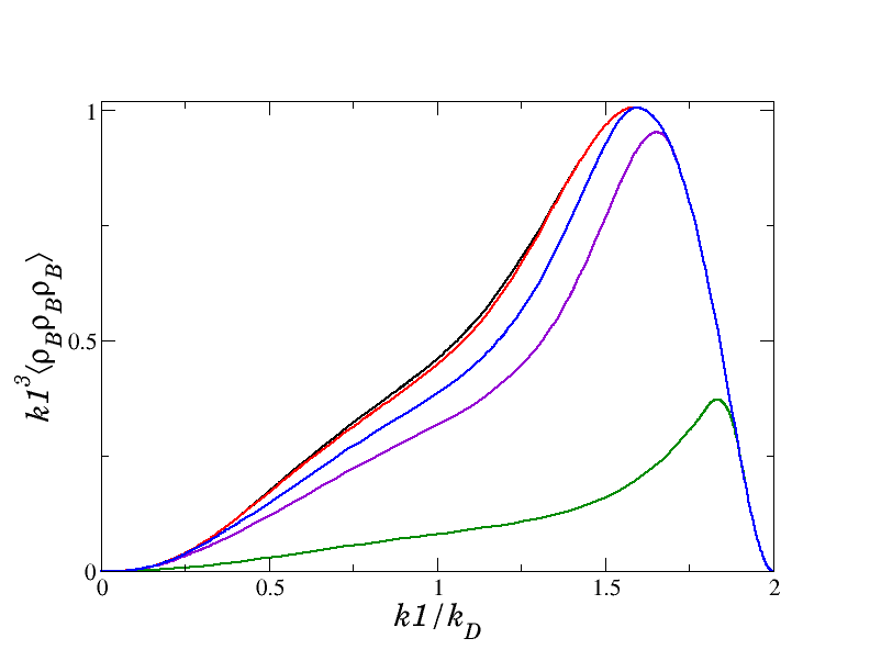
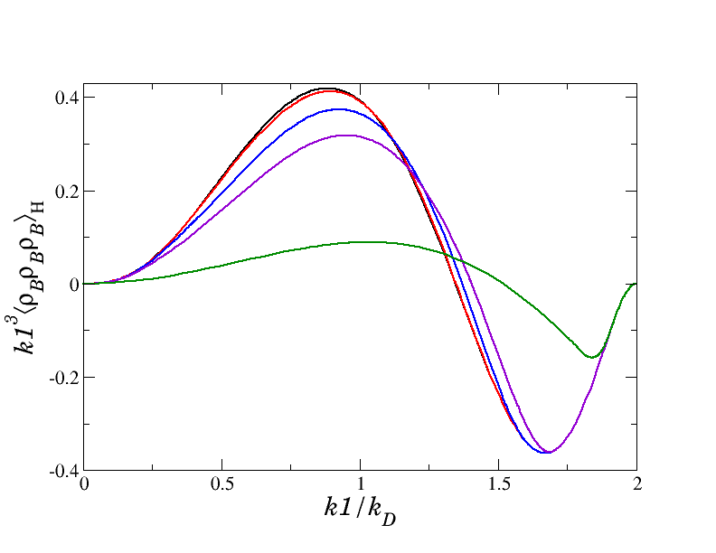
We now analyze the effect of an infrared cut-off parametrized by α𝛼\alpha on the magnetic bispectrum (see equation (2.9)). We saw that the non-Gaussianity peaks at k1k2similar-to𝑘1𝑘2k1\sim k2 under a squeezed configuration, so we compute the magnetic bispectrum using the strategy adopted in [37] and in appendix C. In figure 5, the effect of this IR cut-off for causal fields is illustrated.
Refer to caption
(a) Change of k13ρBρBρB𝑘superscript13delimited-⟨⟩subscript𝜌𝐵subscript𝜌𝐵subscript𝜌𝐵k1^{3}\langle\rho_{B}\rho_{B}\rho_{B}\rangle respect to the infrared cut-off without ABAH2subscript𝐴𝐵superscriptsubscript𝐴𝐻2A_{B}A_{H}^{2}.
Refer to caption
(b) Change of k13ρBρBρB𝑘superscript13delimited-⟨⟩subscript𝜌𝐵subscript𝜌𝐵subscript𝜌𝐵k1^{3}\langle\rho_{B}\rho_{B}\rho_{B}\rangle respect to the infrared cut-off only with ABAH2subscript𝐴𝐵superscriptsubscript𝐴𝐻2A_{B}A_{H}^{2}.
Refer to caption
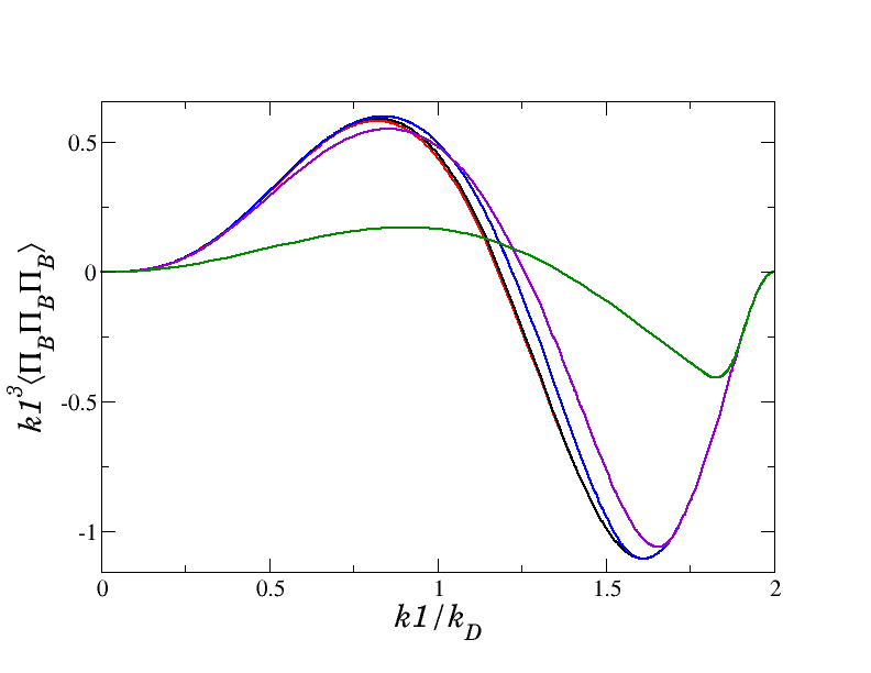
(c) Change of k13ΠBΠBΠB𝑘superscript13delimited-⟨⟩subscriptΠ𝐵subscriptΠ𝐵subscriptΠ𝐵k1^{3}\langle\Pi_{B}\Pi_{B}\Pi_{B}\rangle respect to the infrared cut-off without ABAH2subscript𝐴𝐵superscriptsubscript𝐴𝐻2A_{B}A_{H}^{2}.
Refer to caption
(d) Change of k13ΠBΠBΠB𝑘superscript13delimited-⟨⟩subscriptΠ𝐵subscriptΠ𝐵subscriptΠ𝐵k1^{3}\langle\Pi_{B}\Pi_{B}\Pi_{B}\rangle respect to the infrared cut-off only with ABAH2subscript𝐴𝐵superscriptsubscript𝐴𝐻2A_{B}A_{H}^{2}.
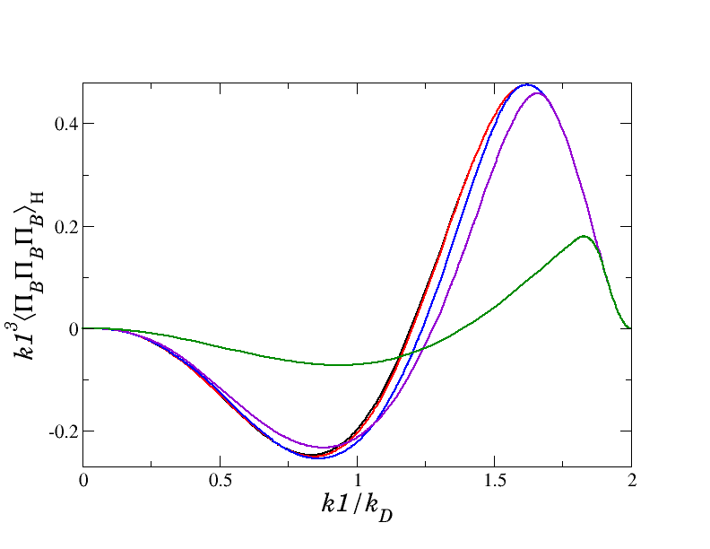
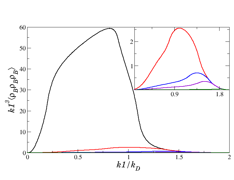
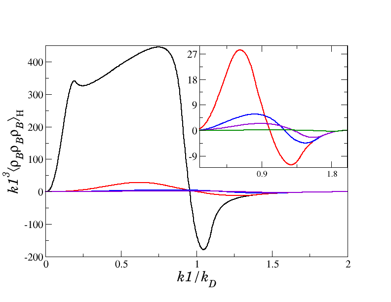
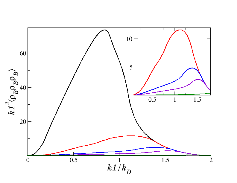
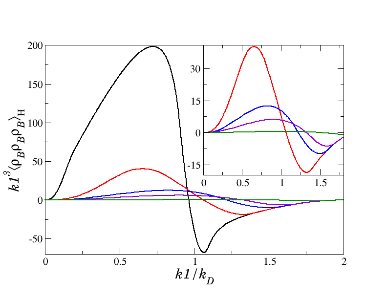
Figure 5: Effects of a lower cut-off at the three-point correlation of non-crossing scalar modes described in the text using the squeezed collinear configuration. The figures (a), (b) show the three-point correlation of the energy density of the magnetic field without and only with ABAH2subscript𝐴𝐵superscriptsubscript𝐴𝐻2A_{B}A_{H}^{2} respectively, while figures (c) and (d) show the three-point correlation of the anisotropic stress of the magnetic field without and only with ABAH2subscript𝐴𝐵superscriptsubscript𝐴𝐻2A_{B}A_{H}^{2} respectively. The black, red, blue, violet and green lines refer to lower cut-off for α=0.01𝛼0.01\alpha=0.01, α=0.4𝛼0.4\alpha=0.4, α=0.6𝛼0.6\alpha=0.6, α=0.7𝛼0.7\alpha=0.7, α=0.9𝛼0.9\alpha=0.9 respectively. Here the units are normalized respect to the values in figure (a) and we use nB=nH=2subscript𝑛𝐵subscript𝑛𝐻2n_{B}=n_{H}=2.
Refer to caption
(a) Change of k13ρBρBρB𝑘superscript13delimited-⟨⟩subscript𝜌𝐵subscript𝜌𝐵subscript𝜌𝐵k1^{3}\langle\rho_{B}\rho_{B}\rho_{B}\rangle respect to the infrared cut-off without ABAH2subscript𝐴𝐵superscriptsubscript𝐴𝐻2A_{B}A_{H}^{2}.
Refer to caption
(b) Change of k13ρBρBρB𝑘superscript13delimited-⟨⟩subscript𝜌𝐵subscript𝜌𝐵subscript𝜌𝐵k1^{3}\langle\rho_{B}\rho_{B}\rho_{B}\rangle respect to the infrared cut-off only with ABAH2subscript𝐴𝐵superscriptsubscript𝐴𝐻2A_{B}A_{H}^{2}.
Refer to caption
(c) Change of k13ρBρBρB𝑘superscript13delimited-⟨⟩subscript𝜌𝐵subscript𝜌𝐵subscript𝜌𝐵k1^{3}\langle\rho_{B}\rho_{B}\rho_{B}\rangle respect to the infrared cut-off without ABAH2subscript𝐴𝐵superscriptsubscript𝐴𝐻2A_{B}A_{H}^{2}.
Refer to caption
(d) Change of k13ρBρBρB𝑘superscript13delimited-⟨⟩subscript𝜌𝐵subscript𝜌𝐵subscript𝜌𝐵k1^{3}\langle\rho_{B}\rho_{B}\rho_{B}\rangle respect to the infrared cut-off only with ABAH2subscript𝐴𝐵superscriptsubscript𝐴𝐻2A_{B}A_{H}^{2}.
Figure 6: Effects of a lower cut-off at the three-point correlation of non-crossing scalar modes described in the text using the squeezed collinear configuration. The figures (a), (b) show the three-point correlation of the energy density of the magnetic field for nB=nH=5/2subscript𝑛𝐵subscript𝑛𝐻52n_{B}=n_{H}=-5/2 without and only with ABAH2subscript𝐴𝐵superscriptsubscript𝐴𝐻2A_{B}A_{H}^{2} respectively, while figures (c) and (d) show the three-point correlation of the energy density of the magnetic field for nB=nH=1.9subscript𝑛𝐵subscript𝑛𝐻1.9n_{B}=n_{H}=-1.9 without and only with ABAH2subscript𝐴𝐵superscriptsubscript𝐴𝐻2A_{B}A_{H}^{2} respectively. The black, red, blue, violet and green lines refer to lower cut-off for α=0.01𝛼0.01\alpha=0.01, α=0.4𝛼0.4\alpha=0.4, α=0.6𝛼0.6\alpha=0.6, α=0.7𝛼0.7\alpha=0.7, α=0.9𝛼0.9\alpha=0.9 respectively. Here the units are normalized respect to the values in figure (5(a)).

The top figures (5(a)) and (5(b)) show the effect of α𝛼\alpha on k13ρBρBρB𝑘superscript13delimited-⟨⟩subscript𝜌𝐵subscript𝜌𝐵subscript𝜌𝐵k1^{3}\langle\rho_{B}\rho_{B}\rho_{B}\rangle where the lines refer to different values of the cut-off, while the bottom figures (5(c)) and (5(d)) show the effect of α𝛼\alpha on k13ΠBΠBΠB𝑘superscript13delimited-⟨⟩subscriptΠ𝐵subscriptΠ𝐵subscriptΠ𝐵k1^{3}\langle\Pi_{B}\Pi_{B}\Pi_{B}\rangle. What we read off these figures is how the peak of the bispectrum moves to high wavenumbers when we increase the value of kmsubscript𝑘𝑚k_{m} in the same way that magnetic power spectrum (and its amplitude decreases also due to reduction of the wavenumber space) and how the effects of the ABAH2subscript𝐴𝐵superscriptsubscript𝐴𝐻2A_{B}A_{H}^{2} contributions PMF are tiny compared with the non-helical case. On the other hand, the figure (6) shows the effect of the infrared cut-off when we are considering non-causal fields. The top panel shows the three-point correlation of the energy density of the magnetic field for nH=nB=5/2subscript𝑛𝐻subscript𝑛𝐵52n_{H}=n_{B}=-5/2 while the bottom panel shows the three-point correlation for nH=nB=1.9subscript𝑛𝐻subscript𝑛𝐵1.9n_{H}=n_{B}=-1.9. Here we can see that the contribution driven by ABAH2subscript𝐴𝐵superscriptsubscript𝐴𝐻2A_{B}A_{H}^{2} is bigger than AB3superscriptsubscript𝐴𝐵3A_{B}^{3}, meaning that for negative spectral indices the effect of helicity becomes relevant for our studies.

5 Reduced Bispectrum from PMF

In this section, we estimate the reduced bispectrum and give a careful review the results of [48],[66],[67]. The CMB temperature perturbation at a direction of photon momentum 𝐧^^𝐧\hat{\mathbf{n}} can be expanded into spherical harmonics

ΔT(Z)T(𝐧^)=lmalm(Z)Ylm(𝐧^),Δsuperscript𝑇𝑍𝑇^𝐧subscript𝑙𝑚subscriptsuperscript𝑎𝑍𝑙𝑚subscript𝑌𝑙𝑚^𝐧\frac{\Delta T^{(Z)}}{T}(\hat{\mathbf{n}})=\sum_{lm}a^{(Z)}_{lm}Y_{lm}(\hat{\mathbf{n}}), (5.1)

where Z=S,V,T𝑍𝑆𝑉𝑇Z=S,V,T refers to the contribution given by scalar , vector or tensor perturbations. The coefficient alm(Z)subscriptsuperscript𝑎𝑍𝑙𝑚a^{(Z)}_{lm} is written as [53]

almZsubscriptsuperscript𝑎𝑍𝑙𝑚\displaystyle a^{Z}_{lm} =\displaystyle= 4π(i)ld3𝐤(2π)3ΔlZ(k)λ[sgn(λ)]λξlm(λ)(k),4𝜋superscript𝑖𝑙superscript𝑑3𝐤superscript2𝜋3subscriptsuperscriptΔ𝑍𝑙𝑘subscript𝜆superscriptdelimited-[]𝑠𝑔𝑛𝜆𝜆superscriptsubscript𝜉𝑙𝑚𝜆𝑘\displaystyle 4\pi(-i)^{l}\int\frac{d^{3}\mathbf{k}}{(2\pi)^{3}}\Delta^{Z}_{l}(k)\sum_{\lambda}[sgn(\lambda)]^{\lambda}\xi_{lm}^{(\lambda)}(k),
ξlm(λ)(k)superscriptsubscript𝜉𝑙𝑚𝜆𝑘\displaystyle\xi_{lm}^{(\lambda)}(k) =\displaystyle= d2𝐤^ξλ(k)λYlm(𝐤^),superscript𝑑2^𝐤superscript𝜉𝜆subscript𝑘𝜆subscriptsuperscript𝑌𝑙𝑚^𝐤\displaystyle\int d^{2}\hat{\mathbf{k}}\xi^{\lambda}(k)_{-\lambda}\!Y^{*}_{lm}(\hat{\mathbf{k}}), (5.2)

where λ=0,±1,±2𝜆0plus-or-minus1plus-or-minus2\lambda=0,\pm 1,\pm 2 describes the helicity of the scalar, vector, tensor mode; Ylmλsubscriptsubscriptsuperscript𝑌𝑙𝑚𝜆{}_{-\lambda}\!Y^{*}_{lm} is the spin-weight spherical harmonics; ξλ(k)superscript𝜉𝜆𝑘\xi^{\lambda}(k) is the primordial perturbation and ΔlZ(k)subscriptsuperscriptΔ𝑍𝑙𝑘\Delta^{Z}_{l}(k) is the transfer function. Let us define the CMB angular bispectrum as

Bl1l2l3m1m2m3=n=13alnmn(Z),superscriptsubscript𝐵subscript𝑙1subscript𝑙2subscript𝑙3subscript𝑚1subscript𝑚2subscript𝑚3delimited-⟨⟩superscriptsubscriptproduct𝑛13superscriptsubscript𝑎subscript𝑙𝑛subscript𝑚𝑛𝑍B_{l_{1}\,l_{2}\,l_{3}}^{m_{1}\,m_{2}\,m_{3}}=\bigg{\langle}\prod_{n=1}^{3}a_{l_{n}\,m_{n}}^{(Z)}\bigg{\rangle}, (5.3)

where only scalar perturbations (Z=S) will be considered in the paper. Now, by substituting the equation (5) into equation (5.3) we can find

n=13alnmn=[n=134π(i)lnd3𝐤𝐧(2π)3Δln(kn)Ylnmn(𝐧^)]×n=13ξ(kn).delimited-⟨⟩superscriptsubscriptproduct𝑛13subscript𝑎subscript𝑙𝑛subscript𝑚𝑛delimited-[]superscriptsubscriptproduct𝑛134𝜋superscript𝑖subscript𝑙𝑛superscript𝑑3𝐤𝐧superscript2𝜋3subscriptΔsubscript𝑙𝑛𝑘𝑛subscriptsuperscript𝑌subscript𝑙𝑛subscript𝑚𝑛^𝐧delimited-⟨⟩superscriptsubscriptproduct𝑛13𝜉𝑘𝑛\bigg{\langle}\prod_{n=1}^{3}a_{l_{n}\,m_{n}}\bigg{\rangle}=\left[\prod_{n=1}^{3}4\pi(-i)^{l_{n}}\int\frac{d^{3}\mathbf{kn}}{(2\pi)^{3}}\Delta_{l_{n}}(kn)Y^{*}_{l_{n}\,m_{n}}(\hat{\mathbf{n}})\right]\times\bigg{\langle}\prod_{n=1}^{3}\xi(kn)\bigg{\rangle}. (5.4)

We also consider a rough approximation for the transfer function that works quite well at large angular scales and for primordial adiabatic perturbations given by Δl(k)=13jl(k(η0η))subscriptΔ𝑙𝑘13subscript𝑗𝑙𝑘subscript𝜂0subscript𝜂\Delta_{l}(k)=\frac{1}{3}j_{l}(k(\eta_{0}-\eta_{*})), where jl(x)subscript𝑗𝑙𝑥j_{l}(x) the spherical Bessel function, η0=14.38subscript𝜂014.38\eta_{0}=14.38 Gpc the conformal time at present and η=284.85subscript𝜂284.85\eta_{*}=284.85 Mpc the conformal time at the recombination epoch [67]. This is the large scale Sachs Wolfe effect. Since we want to evaluate the contribution of the bispectrum by PMFs, the three-point correlator for the primordial perturbation must satisfy the relation

n=13ξ(kn)=APδ(𝐤𝟏+𝐤𝟐+𝐤𝟑)BΠBΠBΠB(S).delimited-⟨⟩superscriptsubscriptproduct𝑛13𝜉𝑘𝑛subscript𝐴𝑃𝛿𝐤𝟏𝐤𝟐𝐤𝟑superscriptsubscript𝐵subscriptΠ𝐵subscriptΠ𝐵subscriptΠ𝐵𝑆\bigg{\langle}\prod_{n=1}^{3}\xi(kn)\bigg{\rangle}=A_{P}\delta(\mathbf{k1}+\mathbf{k2}+\mathbf{k3})B_{\Pi_{B}\Pi_{B}\Pi_{B}}^{(S)}. (5.5)

Here, APsubscript𝐴𝑃A_{P} is a constant that depends on the type of perturbation (passive or compensated magnetic mode) and BΠBΠBΠB(S)superscriptsubscript𝐵subscriptΠ𝐵subscriptΠ𝐵subscriptΠ𝐵𝑆B_{\Pi_{B}\Pi_{B}\Pi_{B}}^{(S)} is the magnetic bispectrum computed above. Using the following relations [66]

δ(𝐤𝟏+𝐤𝟐+𝐤𝟑)=1(2π)3expi(𝐤𝟏+𝐤𝟐+𝐤𝟑)𝐱d3x,𝛿𝐤𝟏𝐤𝟐𝐤𝟑1superscript2𝜋3superscriptsubscriptsuperscript𝑖𝐤𝟏𝐤𝟐𝐤𝟑𝐱superscript𝑑3𝑥\delta(\mathbf{k1}+\mathbf{k2}+\mathbf{k3})=\frac{1}{(2\pi)^{3}}\int_{-\infty}^{\infty}\exp^{i(\mathbf{k1}+\mathbf{k2}+\mathbf{k3})\cdot\mathbf{x}}d^{3}x, (5.6)
expi𝐤𝐱=4πliljl(kx)mYlm(𝐤^)Ylm(𝐱^),superscript𝑖𝐤𝐱4𝜋subscript𝑙superscript𝑖𝑙subscript𝑗𝑙𝑘𝑥subscript𝑚subscript𝑌𝑙𝑚^𝐤superscriptsubscript𝑌𝑙𝑚^𝐱\exp^{i\mathbf{k}\cdot\mathbf{x}}=4\pi\sum_{l}i^{l}j_{l}(kx)\sum_{m}Y_{lm}(\hat{\mathbf{k}})Y_{lm}^{*}(\hat{\mathbf{x}}), (5.7)

with the Gaunt integral 𝒢l1l2l3m1m2m3superscriptsubscript𝒢subscript𝑙1subscript𝑙2subscript𝑙3subscript𝑚1subscript𝑚2subscript𝑚3\mathcal{G}_{l_{1}l_{2}l_{3}}^{m_{1}m_{2}m_{3}} defined by

𝒢l1l2l3m1m2m3superscriptsubscript𝒢subscript𝑙1subscript𝑙2subscript𝑙3subscript𝑚1subscript𝑚2subscript𝑚3\displaystyle\mathcal{G}_{l_{1}l_{2}l_{3}}^{m_{1}m_{2}m_{3}} \displaystyle\equiv d2𝐧^Yl1m1(𝐧^)Yl2m2(𝐧^)Yl3m3(𝐧^)superscript𝑑2^𝐧subscript𝑌subscript𝑙1subscript𝑚1^𝐧subscript𝑌subscript𝑙2subscript𝑚2^𝐧subscript𝑌subscript𝑙3subscript𝑚3^𝐧\displaystyle\int d^{2}\hat{\mathbf{n}}Y_{l_{1}m_{1}}(\hat{\mathbf{n}})Y_{l_{2}m_{2}}(\hat{\mathbf{n}})Y_{l_{3}m_{3}}(\hat{\mathbf{n}}) (5.12)
=\displaystyle= (2l1+1)(2l2+1)(2l3+1)4π(l1l2l3000)(l1l2l3m1m2m3),2subscript𝑙112subscript𝑙212subscript𝑙314𝜋subscript𝑙1subscript𝑙2subscript𝑙3000subscript𝑙1subscript𝑙2subscript𝑙3subscript𝑚1subscript𝑚2subscript𝑚3\displaystyle\sqrt{\frac{(2l_{1}+1)(2l_{2}+1)(2l_{3}+1)}{4\pi}}\bigg{(}\begin{array}[]{ccc}l_{1}&l_{2}&l_{3}\\ 0&0&0\end{array}\bigg{)}\bigg{(}\begin{array}[]{ccc}l_{1}&l_{2}&l_{3}\\ m_{1}&m_{2}&m_{3}\end{array}\bigg{)},

and along with the equation (5.5), the equation (5.4) takes the form

n=13alnmndelimited-⟨⟩superscriptsubscriptproduct𝑛13subscript𝑎subscript𝑙𝑛subscript𝑚𝑛\displaystyle\bigg{\langle}\prod_{n=1}^{3}a_{l_{n}\,m_{n}}\bigg{\rangle} =\displaystyle= AP(2l1+1)(2l2+1)(2l3+1)4π(l1l2l3000)(l1l2l3m1m2m3)×\displaystyle A_{P}\sqrt{\frac{(2l_{1}+1)(2l_{2}+1)(2l_{3}+1)}{4\pi}}\bigg{(}\begin{array}[]{ccc}l_{1}&l_{2}&l_{3}\\ 0&0&0\end{array}\bigg{)}\bigg{(}\begin{array}[]{ccc}l_{1}&l_{2}&l_{3}\\ m_{1}&m_{2}&m_{3}\end{array}\bigg{)}\times (5.17)
×\displaystyle\times [n=1313π2kn2jln(knx)jln(kn(η0η))𝑑kn]BΠBΠBΠB(S)x2dx.delimited-[]superscriptsubscriptproduct𝑛1313superscript𝜋2𝑘superscript𝑛2subscript𝑗subscript𝑙𝑛𝑘𝑛𝑥subscript𝑗subscript𝑙𝑛𝑘𝑛subscript𝜂0subscript𝜂differential-d𝑘𝑛superscriptsubscript𝐵subscriptΠ𝐵subscriptΠ𝐵subscriptΠ𝐵𝑆superscript𝑥2𝑑𝑥\displaystyle\left[\prod_{n=1}^{3}\frac{1}{3\pi^{2}}\int kn^{2}\int j_{l_{n}}(kn\,x)j_{l_{n}}(kn(\eta_{0}-\eta_{*}))dkn\right]B_{\Pi_{B}\Pi_{B}\Pi_{B}}^{(S)}x^{2}dx. (5.18)

Here the matrix is the Wigner-3j symbol and it vanishes unless the selection rules are satisfied444The Wigner-3j symbols satisfy that: |m1|l1subscript𝑚1subscript𝑙1|m_{1}|\leq l_{1}, |m2|l2subscript𝑚2subscript𝑙2|m_{2}|\leq l_{2}, |m3|l3subscript𝑚3subscript𝑙3|m_{3}|\leq l_{3}, m1+m2+m3=0subscript𝑚1subscript𝑚2subscript𝑚30m_{1}+m_{2}+m_{3}=0, l1+l2+l3=subscript𝑙1subscript𝑙2subscript𝑙3l_{1}+l_{2}+l_{3}=\mathbb{Z} and |l1l2|l3l1+l2subscript𝑙1subscript𝑙2subscript𝑙3subscript𝑙1subscript𝑙2|l_{1}-l_{2}|\leq l_{3}\leq l_{1}+l_{2} [53]. . Given the rotational invariance of the Universe, Komatsu-Spergel [66] defined a real symmetric function of lisubscript𝑙𝑖l_{i} called the reduced bispectrum bl1l2l3subscript𝑏subscript𝑙1subscript𝑙2subscript𝑙3b_{l_{1}l_{2}l_{3}}

n=13alnmn𝒢l1l2l3m1m2m3bl1l2l3.delimited-⟨⟩superscriptsubscriptproduct𝑛13subscript𝑎subscript𝑙𝑛subscript𝑚𝑛superscriptsubscript𝒢subscript𝑙1subscript𝑙2subscript𝑙3subscript𝑚1subscript𝑚2subscript𝑚3subscript𝑏subscript𝑙1subscript𝑙2subscript𝑙3\bigg{\langle}\prod_{n=1}^{3}a_{l_{n}\,m_{n}}\bigg{\rangle}\equiv\mathcal{G}_{l_{1}l_{2}l_{3}}^{m_{1}m_{2}m_{3}}b_{l_{1}l_{2}l_{3}}. (5.19)

Checking the last two equations, the properties of the bispectrum generated by PMFs can be expressed via the reduced bispectrum as

bl1l2l3=AP[n=1313π2kn2jln(knx)jln(kn(η0η))𝑑kn]BΠBΠBΠB(S)x2dx.subscript𝑏subscript𝑙1subscript𝑙2subscript𝑙3subscript𝐴𝑃delimited-[]superscriptsubscriptproduct𝑛1313superscript𝜋2𝑘superscript𝑛2subscript𝑗subscript𝑙𝑛𝑘𝑛𝑥subscript𝑗subscript𝑙𝑛𝑘𝑛subscript𝜂0subscript𝜂differential-d𝑘𝑛superscriptsubscript𝐵subscriptΠ𝐵subscriptΠ𝐵subscriptΠ𝐵𝑆superscript𝑥2𝑑𝑥\displaystyle b_{l_{1}l_{2}l_{3}}=A_{P}\left[\prod_{n=1}^{3}\frac{1}{3\pi^{2}}\int kn^{2}\int j_{l_{n}}(kn\,x)j_{l_{n}}(kn(\eta_{0}-\eta_{*}))dkn\right]B_{\Pi_{B}\Pi_{B}\Pi_{B}}^{(S)}x^{2}dx. (5.20)

In order to calculate APsubscript𝐴𝑃A_{P}, we must clarify the sources of primordial perturbations. Prior to neutrino decoupling (τν=1subscript𝜏𝜈1\tau_{\nu}=1MeV-1), the Universe is dominated by radiation and it is tightly coupled to baryons such that they cannot have any anisotropic stress contribution. Since we are also considering magnetic fields, they would be the only ones that develop anisotropic stress and therefore at superhorizon scales the curvature perturbation depends on the primordial magnetic source[53]. But after neutrino decoupling, neutrinos generated anisotropic stress which compensates the one coming from PMF finishing the growth of the perturbations. Shaw-Lewis [68] showed that curvature perturbation is given by

ξ(k)13Rγln(τντB)ΠB(S)(k),similar-to𝜉𝑘13subscript𝑅𝛾subscript𝜏𝜈subscript𝜏𝐵superscriptsubscriptΠ𝐵𝑆𝑘\xi(k)\sim-\frac{1}{3}R_{\gamma}\ln\left(\frac{\tau_{\nu}}{\tau_{B}}\right)\Pi_{B}^{(S)}(k), (5.21)

commonly known as passive mode, where Rγ=ργρ0.6subscript𝑅𝛾subscript𝜌𝛾𝜌similar-to0.6R_{\gamma}=\frac{\rho_{\gamma}}{\rho}\sim 0.6 and τBsubscript𝜏𝐵\tau_{B} is the epoch of magnetic field generation. Another contribution comes from the density-sourced mode with unperturbed anisotropic stresses, the magnetic compensated scalar mode, this is proportional to the amplitude of the perturbed magnetic density just as the magnetic Sachs Wolfe effect [68]. So, if the primordial perturbation is associated with the initial gravitational potential, in the limit on large-angular scales the compensated modes is expressed as [48, 69]

ξ(k)14RγρB(k).similar-to𝜉𝑘14subscript𝑅𝛾subscript𝜌𝐵𝑘\xi(k)\sim\frac{1}{4}R_{\gamma}\rho_{B}(k). (5.22)

Therefore if we use the passive mode contribution, BΠBΠBΠB(S)superscriptsubscript𝐵subscriptΠ𝐵subscriptΠ𝐵subscriptΠ𝐵𝑆B_{\Pi_{B}\Pi_{B}\Pi_{B}}^{(S)} is given by BΠB(S)ΠB(S)ΠB(S)(S)superscriptsubscript𝐵superscriptsubscriptΠ𝐵𝑆superscriptsubscriptΠ𝐵𝑆superscriptsubscriptΠ𝐵𝑆𝑆B_{\Pi_{B}^{(S)}\Pi_{B}^{(S)}\Pi_{B}^{(S)}}^{(S)} (see equation (3.12)) with AP=(13Rγln(τντB))3subscript𝐴𝑃superscript13subscript𝑅𝛾subscript𝜏𝜈subscript𝜏𝐵3A_{P}=\left(-\frac{1}{3}R_{\gamma}\ln\left(\frac{\tau_{\nu}}{\tau_{B}}\right)\right)^{3}, whilst compensated mode the primordial three-point correlation is described by BρBρBρB(S)superscriptsubscript𝐵subscript𝜌𝐵subscript𝜌𝐵subscript𝜌𝐵𝑆B_{\rho_{B}\rho_{B}\rho_{B}}^{(S)} (see equation (3.6)) with AP=(14Rγ)3subscript𝐴𝑃superscript14subscript𝑅𝛾3A_{P}=\left(\frac{1}{4}R_{\gamma}\right)^{3}. Since the magnetic bispectrum only depends on (k1;k2)𝑘1𝑘2(k1;k2), the k3𝑘3k3 integral in the equation (5.20) gives π2x2δ(x(η0η))𝜋2superscript𝑥2𝛿𝑥subscript𝜂0subscript𝜂\frac{\pi}{2x^{2}}\delta(x-(\eta_{0}-\eta_{*})) due to the closure relation [48], and integrating out the delta function one finally obtains

bl1l2l3=APπ2[n=1213π2kn2jln(kn(η0η))2𝑑kn]BΠBΠBΠB(S).subscript𝑏subscript𝑙1subscript𝑙2subscript𝑙3subscript𝐴𝑃𝜋2delimited-[]superscriptsubscriptproduct𝑛1213superscript𝜋2𝑘superscript𝑛2subscript𝑗subscript𝑙𝑛superscript𝑘𝑛subscript𝜂0subscript𝜂2differential-d𝑘𝑛superscriptsubscript𝐵subscriptΠ𝐵subscriptΠ𝐵subscriptΠ𝐵𝑆\displaystyle b_{l_{1}l_{2}l_{3}}=A_{P}\frac{\pi}{2}\left[\prod_{n=1}^{2}\frac{1}{3\pi^{2}}\int kn^{2}j_{l_{n}}(kn(\eta_{0}-\eta_{*}))^{2}dkn\right]B_{\Pi_{B}\Pi_{B}\Pi_{B}}^{(S)}. (5.23)

This is the master formula that we shall use in the following section in order to calculate the CMB reduced bispectrum.

6 Analysis

In this section we show the numerical results of the CMB reduced bispectrum produced by helical PMFs. In order to numerically solve eq.(5.23), we use the adaptive strategy implemented in Mathematica called Levin-type rule which estimates the integral of an oscillatory function with a good accuracy[73].

6.1 Causal Fields

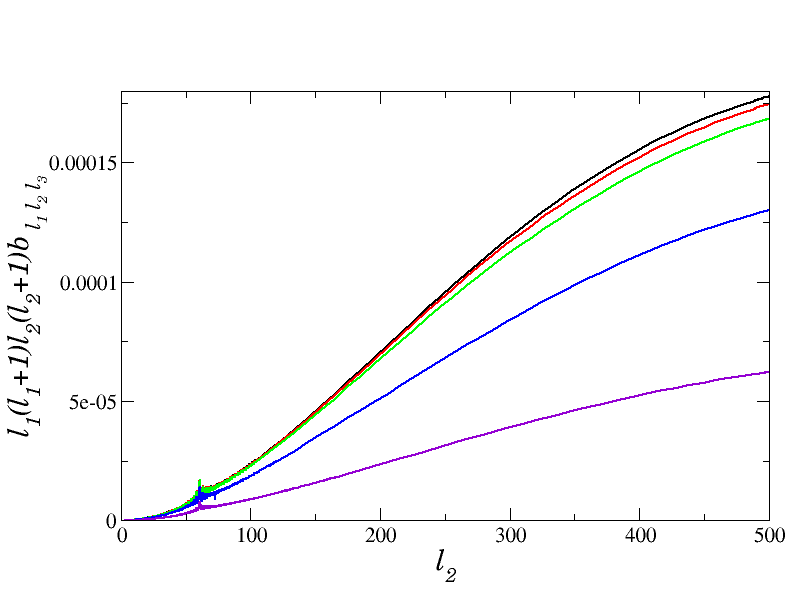
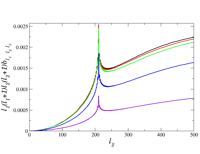
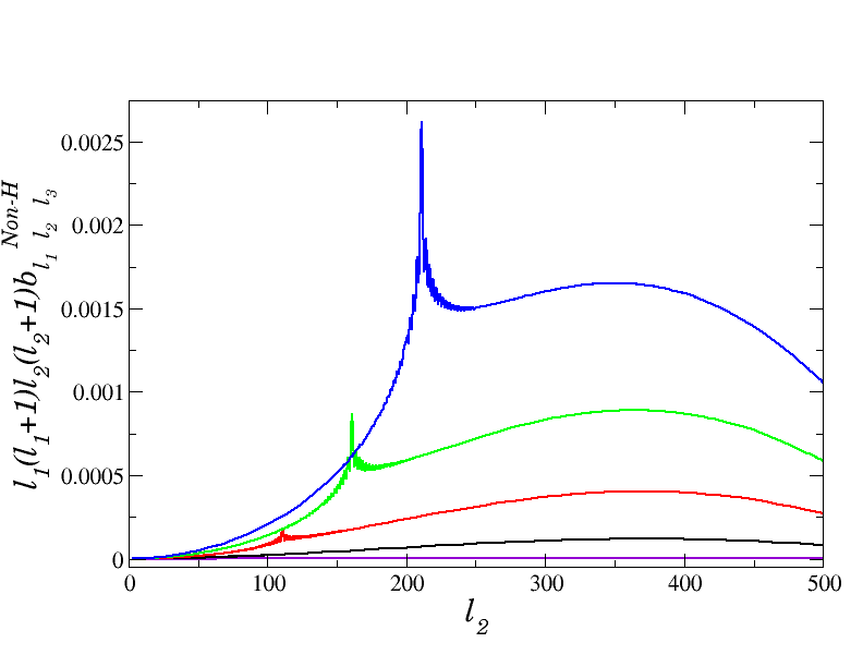
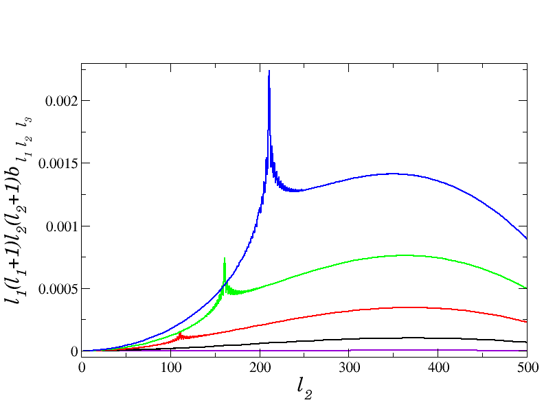
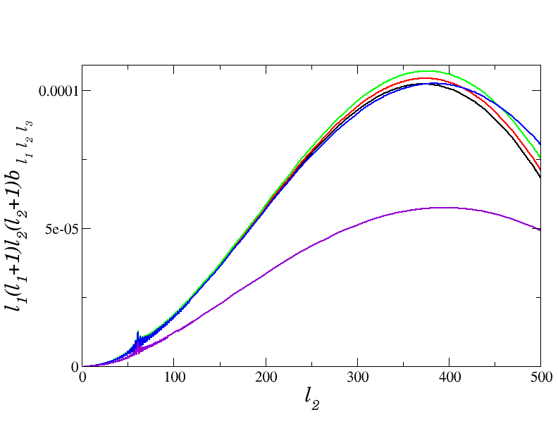
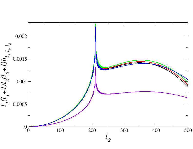
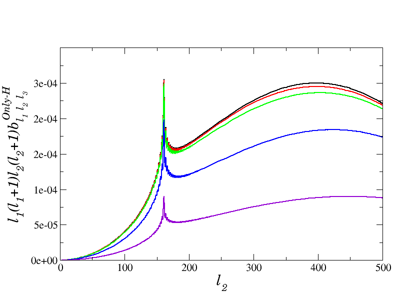
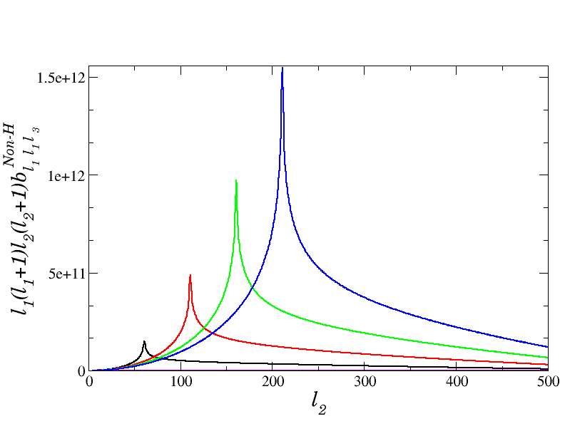
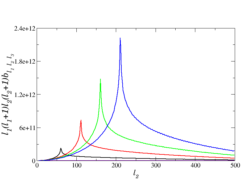
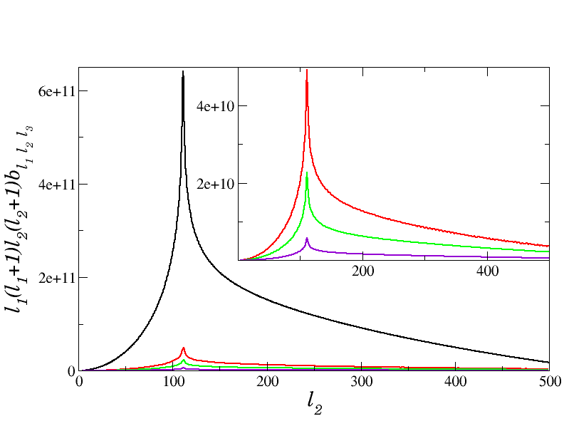
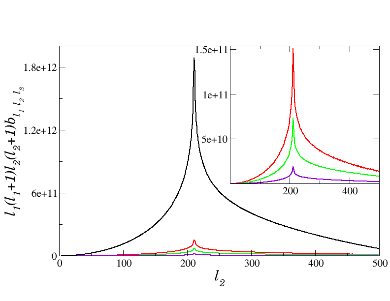
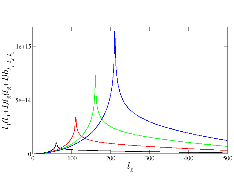
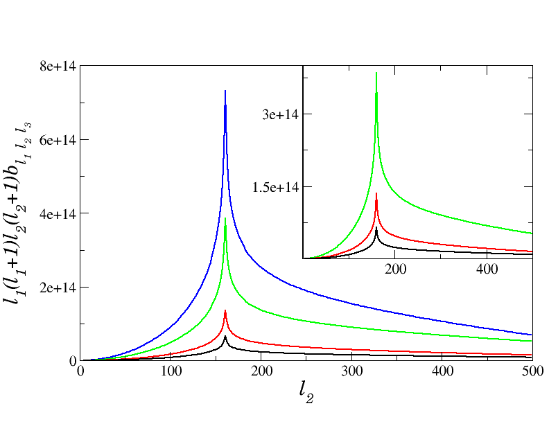
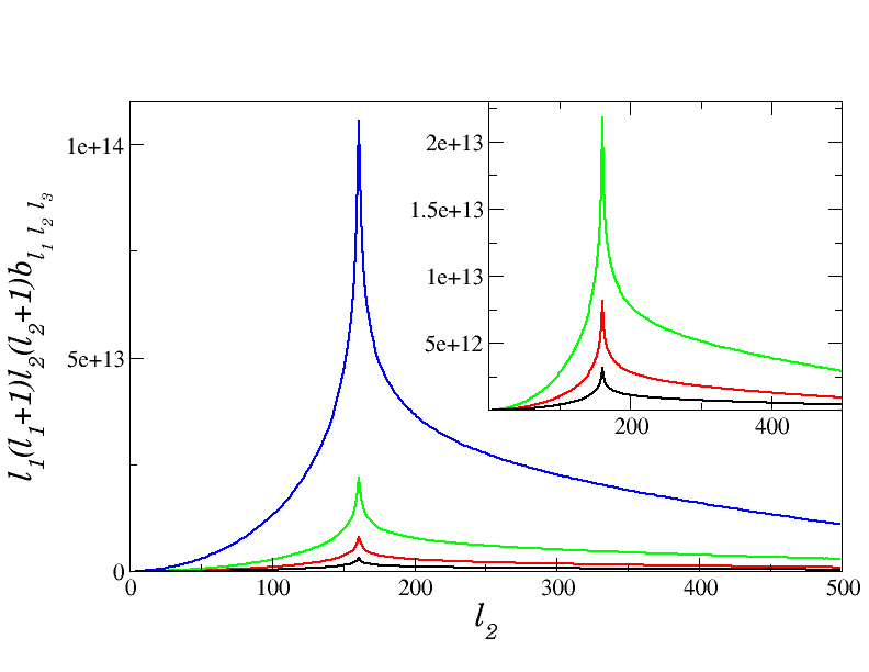
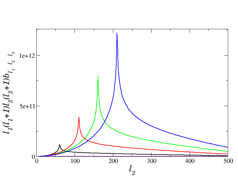
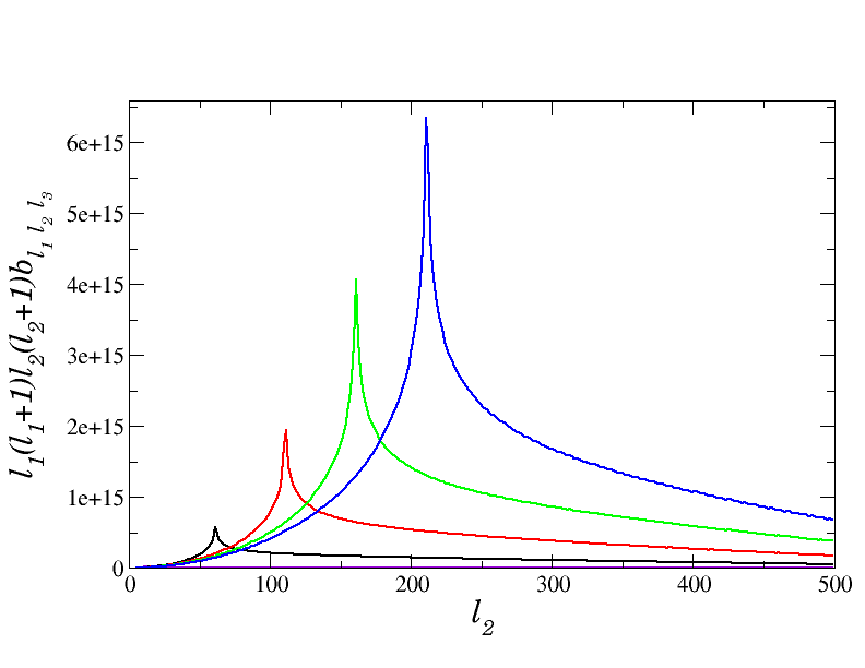
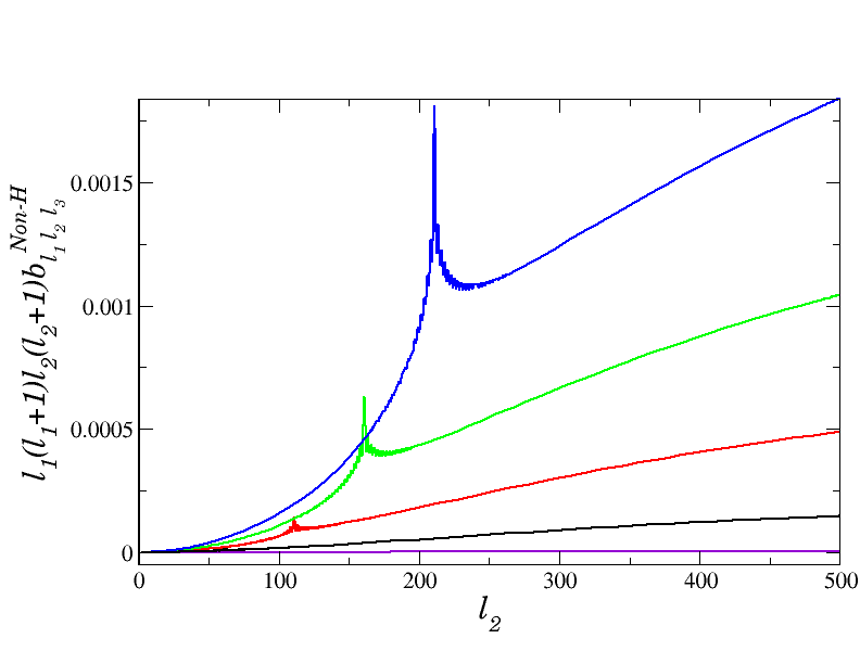
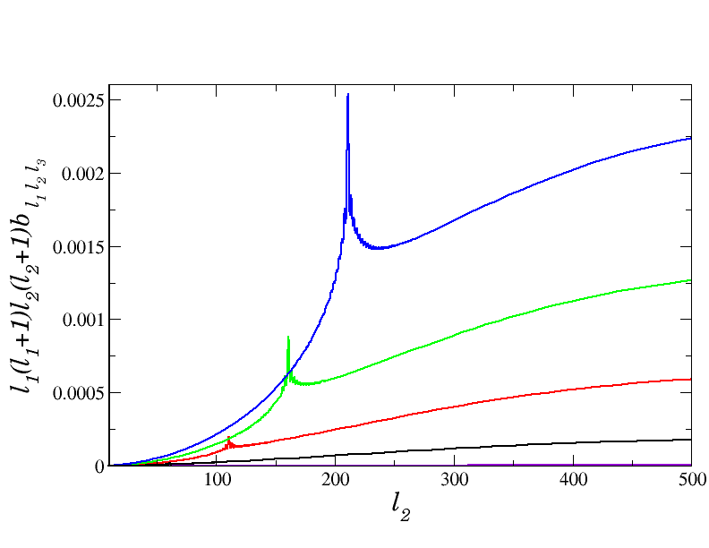
Figure 7 presents the CMB reduced bispectrum generated by compensated PMFs modes under collinear configuration. In this figure we observe the signal produced by only the AB3superscriptsubscript𝐴𝐵3A_{B}^{3} contribution (7(a)), as welll as the signal by the whole(7(b)). We found that ABAH2subscript𝐴𝐵superscriptsubscript𝐴𝐻2A_{B}A_{H}^{2} contribution (helical) is smaller than non-helical part AB3superscriptsubscript𝐴𝐵3A_{B}^{3}. Here we plot the change of the reduced bispectrum with respect to l1subscript𝑙1l_{1}, finding a large contribution for larges values of l1subscript𝑙1l_{1}. We also see that helical contribution reaches a maximum around l2400similar-tosubscript𝑙2400l_{2}\sim 400 whilst non-helical contribution tends to increase at least until l2500similar-tosubscript𝑙2500l_{2}\sim 500. In figures (7(c)) and (7(d)), the effect of an IR cut-off on the reduced bispectrum are shown. Each of these plots show the signal for different values of l1subscript𝑙1l_{1}. We see that signal is biggest for small α𝛼\alpha values (being the biggest contribution for spectrum without IR cut-off) similar to the found with the power spectrum case[37].
Refer to caption
(a) Reduced bispectrum given by AB3superscriptsubscript𝐴𝐵3A_{B}^{3} contribution of compensated PMFs.
Refer to caption
(b) Reduced bispectrum given by total contribution of compensated PMFs.
Refer to caption
(c) Effects of infrared cut-off on the reduced bispectrum with l1=61subscript𝑙161l_{1}=61.
Refer to caption
(d) Effects of infrared cut-off on the reduced bispectrum with l1=210subscript𝑙1210l_{1}=210.
Figure 7: Reduced bispectrum seeded by compensated PMFs with n=2𝑛2n=2 using the squeezed collinear configuration. The figures (a) shows the reduced bispectrum of the magnetic field with only AB3superscriptsubscript𝐴𝐵3A_{B}^{3}, while figure (b) shows the total contribution of the compensated mode; here the lines refers to different values of l1subscript𝑙1l_{1}, violet(l1=11subscript𝑙111l_{1}=11), black(l1=61subscript𝑙161l_{1}=61), red(l1=110subscript𝑙1110l_{1}=110), green(l1=161subscript𝑙1161l_{1}=161) and blue line(l1=210subscript𝑙1210l_{1}=210). The figures (c), (d) show the effects of an infrared cut-off on the reduced bispectrum for different values of multipolar numbers l1subscript𝑙1l_{1}. Black; red; green; blue; and violet lines refer to lower cut-off of α=0.001𝛼0.001\alpha=0.001, α=0.4𝛼0.4\alpha=0.4, α=0.5𝛼0.5\alpha=0.5, α=0.7𝛼0.7\alpha=0.7, α=0.8𝛼0.8\alpha=0.8 respectively. The reduced bispectrum is in units of 4π108AP/(8π2ργ,0)34𝜋superscript108subscript𝐴𝑃superscript8superscript𝜋2subscript𝜌𝛾034\pi 10^{-8}A_{P}/(8\pi^{2}\rho_{\gamma,0})^{3}.
Refer to caption
(a) Reduced bispectrum given by only AB3superscriptsubscript𝐴𝐵3A_{B}^{3} contribution of passive PMFs.
Refer to caption
(b) Reduced bispectrum given by total contribution of passive PMFs.
Refer to caption
(c) Effects of infrared cut-off on the reduced bispectrum with l1=61subscript𝑙161l_{1}=61.
Refer to caption
(d) Effects of infrared cut-off on the reduced bispectrum with l1=210subscript𝑙1210l_{1}=210.
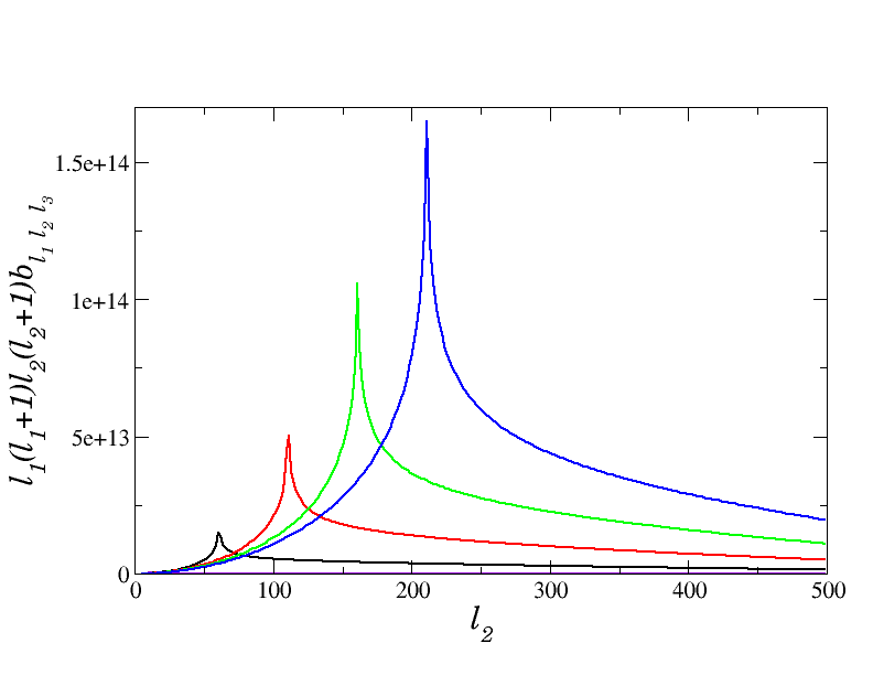
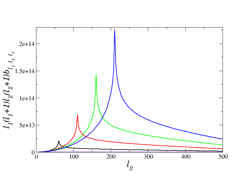
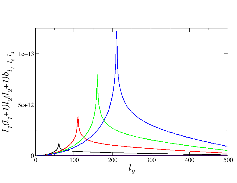
Figure 8: Reduced bispectrum seeded by passive PMFs with nB=nH=n=2subscript𝑛𝐵subscript𝑛𝐻𝑛2n_{B}=n_{H}=n=2 using the squeezed collinear configuration. The figure (a) shows reduced bispectrum of the magnetic field with only AB3superscriptsubscript𝐴𝐵3A_{B}^{3}, while figure (b) shows the total contribution of the passive mode, here the lines refer to different values of l1subscript𝑙1l_{1}, violet(l1=11subscript𝑙111l_{1}=11), black(l1=61subscript𝑙161l_{1}=61), red(l1=110subscript𝑙1110l_{1}=110), green(l1=161subscript𝑙1161l_{1}=161) and blue line(l1=210subscript𝑙1210l_{1}=210). The figures (c) and (d) show the effects of an infrared cut-off on the reduced bispectrum for difference values of multipolar numbers l1subscript𝑙1l_{1}. Black; red; green; blue; and violet lines refer to lower cut-off of α=0.001𝛼0.001\alpha=0.001, α=0.4𝛼0.4\alpha=0.4, α=0.5𝛼0.5\alpha=0.5, α=0.7𝛼0.7\alpha=0.7, α=0.8𝛼0.8\alpha=0.8 respectively. The reduced bispectrum is in units of 4π108AP/2(8π2ργ,0)34𝜋superscript108subscript𝐴𝑃2superscript8superscript𝜋2subscript𝜌𝛾034\pi 10^{-8}A_{P}/2(8\pi^{2}\rho_{\gamma,0})^{3}.
Refer to caption
(a) Effects of infrared cut-off on the reduced bispectrum with l1=161subscript𝑙1161l_{1}=161 seeded by total contribution of compensated helical PMFs.
Refer to caption
(b) Effects of infrared cut-off on the reduced bispectrum with l1=161subscript𝑙1161l_{1}=161 seeded by total contribution of passive helical PMFs.
Figure 9: Reduced bispectrum seeded by compensated (a) and passive (b) helical PMFs with only ABAH2subscript𝐴𝐵superscriptsubscript𝐴𝐻2A_{B}A_{H}^{2} contribution using the squeezed collinear configuration. Black; red; green; blue; and violet lines refer to lower cut-off of α=0.001𝛼0.001\alpha=0.001, α=0.4𝛼0.4\alpha=0.4, α=0.5𝛼0.5\alpha=0.5, α=0.7𝛼0.7\alpha=0.7, α=0.8𝛼0.8\alpha=0.8 respectively. The reduced bispectrum is in units of 4π108AP/2(8π2ργ,0)34𝜋superscript108subscript𝐴𝑃2superscript8superscript𝜋2subscript𝜌𝛾034\pi 10^{-8}A_{P}/2(8\pi^{2}\rho_{\gamma,0})^{3}.
Refer to caption
(a) Reduced bispectrum given by AB3superscriptsubscript𝐴𝐵3A_{B}^{3} contribution of compensated PMFs.
Refer to caption
(b) Reduced bispectrum given by total contribution of compensated PMFs.
Refer to caption
(c) Effects of infrared cut-off on the reduced bispectrum with l1=111subscript𝑙1111l_{1}=111.
Refer to caption
(d) Effects of infrared cut-off on the reduced bispectrum with l1=210subscript𝑙1210l_{1}=210.
Figure 10: Absolute value of reduced bispectrum seeded by compensated PMFs with n=5/2𝑛52n=-5/2 using the squeezed collinear configuration. The figure (a) shows reduced bispectrum of the magnetic field with only AB3superscriptsubscript𝐴𝐵3A_{B}^{3} contribution, while figure (b) shows the total contribution of the compensated mode; here the lines refers to different values of l1subscript𝑙1l_{1}, violet(l1=11subscript𝑙111l_{1}=11), black(l1=61subscript𝑙161l_{1}=61), red(l1=110subscript𝑙1110l_{1}=110), green(l1=161subscript𝑙1161l_{1}=161) and blue line(l1=210subscript𝑙1210l_{1}=210). The figures (c) and (d) show the effects of an infrared cut-off on the reduced bispectrum for difference values of multipolar numbers l1subscript𝑙1l_{1}. Black; red; green; and violet lines refer to lower cut-off of α=0.001𝛼0.001\alpha=0.001, α=0.4𝛼0.4\alpha=0.4, α=0.6𝛼0.6\alpha=0.6, α=0.8𝛼0.8\alpha=0.8 respectively. The reduced bispectrum is in units of 4π1016AP/(8π2ργ,0)34𝜋superscript1016subscript𝐴𝑃superscript8superscript𝜋2subscript𝜌𝛾034\pi 10^{16}A_{P}/(8\pi^{2}\rho_{\gamma,0})^{3}.
Refer to caption
(a) Reduced bispectrum of compensated PMFs for n=3/2𝑛32n=-3/2.
Refer to caption
(b) Reduced bispectrum of compensated PMFs for n=1.9𝑛1.9n=-1.9.
Refer to caption
(c) Effects of infrared cut-off on the reduced bispectrum with l1=161subscript𝑙1161l_{1}=161 for n=3/2𝑛32n=-3/2.
Refer to caption
(d) Effects of infrared cut-off on the reduced bispectrum with l1=161subscript𝑙1161l_{1}=161 for n=1.9𝑛1.9n=-1.9.
Figure 11: Absolute values of reduced bispectrum seeded by compensated PMFs using the squeezed collinear configuration. The figures (a), (b) show the total contribution of the compensated mode of the magnetic field for n=3/2𝑛32n=-3/2 and n=1.9𝑛1.9n=-1.9 respectively; here the lines refers to different values of l1subscript𝑙1l_{1}, violet(l1=11subscript𝑙111l_{1}=11), black(l1=61subscript𝑙161l_{1}=61), red(l1=110subscript𝑙1110l_{1}=110), green(l1=161subscript𝑙1161l_{1}=161) and blue line(l1=210subscript𝑙1210l_{1}=210). The last figures (c),(d) show the effects of an infrared cut-off on the reduced bispectrum for difference values of multipolar numbers l1subscript𝑙1l_{1}. Blue; green; red; and black lines refer to lower cut-off of α=0.001𝛼0.001\alpha=0.001, α=0.4𝛼0.4\alpha=0.4, α=0.6𝛼0.6\alpha=0.6, α=0.8𝛼0.8\alpha=0.8, respectively. The bispectrum is in units of 4π1016AP/(8π2ργ,0)34𝜋superscript1016subscript𝐴𝑃superscript8superscript𝜋2subscript𝜌𝛾034\pi 10^{16}A_{P}/(8\pi^{2}\rho_{\gamma,0})^{3}.
Refer to caption
(a) Reduced bispectrum of compensated PMFs for n=5/2𝑛52n=-5/2.
Refer to caption
(b) Reduced bispectrum of compensated PMFs for n=3/2𝑛32n=-3/2.
Refer to caption
(c) Reduced bispectrum of passive PMFs for n=5/2𝑛52n=-5/2.
Refer to caption
(d) Reduced bispectrum of passive PMFs for n=3/2𝑛32n=-3/2.
Figure 12: Absolute values of reduced bispectrum seeded by passive and compensated PMFs under p-independent approximation. The figures (a), (b) show the total contribution of the compensated mode of the magnetic field for n=5/2𝑛52n=-5/2 and n=3/2𝑛32n=-3/2 respectively. The figures (c), (d) show the total contribution of the passive mode of the magnetic field for n=5/2𝑛52n=-5/2 and n=3/2𝑛32n=-3/2 respectively. Here the lines refer to different values of l1subscript𝑙1l_{1}, violet(l1=11subscript𝑙111l_{1}=11), black(l1=61subscript𝑙161l_{1}=61), red(l1=110subscript𝑙1110l_{1}=110), green(l1=161subscript𝑙1161l_{1}=161) and blue line(l1=210subscript𝑙1210l_{1}=210).

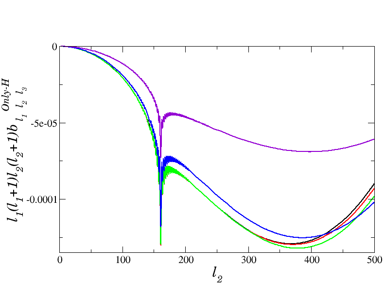
In Figure (8) we show the CMB reduced bispectrum generated by PMFs passive modes under collinear configuration. Meanwhile, figures (8(a)) and (8(b)) describe the signal for the non-helical and total contribution respectively. An interesting feature is that reduced bispectrum generated by helical contribution is totally negative, then, by using this unusual behavior we would have direct evidence of a helical component in the field.

Other important result of this paper is reported in figures (8(c)) and (8(d)). Here we show again the effect of an IR cut-off on the reduced bispectrum and we have found out that the biggest contribution of the bispectrum comes from an IR cut-off near α0.5similar-to𝛼0.5\alpha\sim 0.5 instead of α=0𝛼0\alpha=0. This peak might correspond to a type of dynamics in large scales and help us to determine the nature of PMFs (Since we are trying with causal fields, this infrared cut-off would correspond to the maximum scale in which magnetic fields may be generated at later times). Therefore the evidence of this cut-off in the bispectrum would reveal an interesting signal from passive magnetic scalar mode. In addition, the change of the reduced bispectrum for helical PMFs in presence of an IR cut-off is showed in figure (9). Here we observe how the signal decreases when the IR cut-off increases for the compensated mode and how change the behavior for the passive case. We want to remark on some approximations used so far. Since we assume that effects of PMFs are important for small multipolar numbers, we write the transfer functions in terms of spherical Bessel function. Previous papers have worked without this approximation. For instance, [55] computes the full radiation transfer function taking into account the effect of PMFs. The full numerical integration of the bispectrum can be done via second-order Einstein-Boltzmann codes like SONG[74] improving the estimation of the amplitude of PMFs. Moreover, we must note that [70] found a WMAP bound on non-helical passive mode for tensor temperature bispectrum of B1Mpc<3.1subscript𝐵1𝑀𝑝𝑐3.1B_{1Mpc}<3.1nG and the Planck paper [56] reported B1Mpc<2.8subscript𝐵1𝑀𝑝𝑐2.8B_{1Mpc}<2.8nG all of them for scale-invariant fields. Actually, the tensor mode is dominant in the passive mode, and can give quite tighter constraint of the PMF amplitude than the scalar mode. Thus, tensor mode contribution and a full transfer function determined by the presence of these fields will improve our results and therefore they will be interesting subjects of our future work.

6.2 Non-causal Fields

Now let us consider a red magnetic spectrum. Figure (10) shows the reduced bispectrum for compensated mode with nH=nB=n=5/2subscript𝑛𝐻subscript𝑛𝐵𝑛52n_{H}=n_{B}=n=-5/2. Again, we plot the non-helical (10(a)) and total (10(b)) contribution of the bispectrum while plots (10(c)) and (10(d)) correspond to the change of the signal due to an IR cut-off. Since the PMFs bispectrum is almost determined by the poles in each k𝑘k, the value of it peaked for l1=l2=l3subscript𝑙1subscript𝑙2subscript𝑙3l_{1}=l_{2}=l_{3} as we can observe in figures (10),(11), (12). Additionally, the figure (11) shows signals for nH=nB=n=3/2subscript𝑛𝐻subscript𝑛𝐵𝑛32n_{H}=n_{B}=n=-3/2 and nH=nB=n=1.9subscript𝑛𝐻subscript𝑛𝐵𝑛1.9n_{H}=n_{B}=n=-1.9. As a matter of fact, some mechanisms of inflationary magnetogenesis with parity violating terms which lead to helical magnetic field (n=1.9𝑛1.9n=-1.9), stand for the lower bound for the which the field can satisfy the intensity of magnetic fields in the intergalactic medium; thereby the signal described in figure (11) constraints models for providing the seed for galactic magnetic fields [29]. On the other hand, figure (12) shows the reduced bispectrum taking into account the p-independent approximation implemented in section 4.1. Due to complexity of the angular structure on the PMF bispectrum for passive mode, the numerical computation for reduced bispectrum requires a great deal of time. To avoid this problem we can use the p-independent approximation by reducing the PMF bispectrum to an independent angular form as we studied above. From figures (12(a)) and (12(b)) we observe an increase in the signal as we expected due to the lack of angular terms in the bispectrum. Finally, figures (12(c)) and (12(d)) show the total contribution of passive modes. Note that the amplitude is larger than the compensated mode. This behavior have also been reported in [48]. This result is interesting because an estimation of Bλsubscript𝐵𝜆B_{\lambda} through a local-type primordial NG in curvature perturbation generates constraints stronger than the compensated ones. Finally, if we compare the results reported in this section with the ones shown in above section for causal fields, we can observe that effect of kmsubscript𝑘𝑚k_{m} is more significant in negative spectral indices, specially for nearly scale invariant scale fields. We then conclude that kmsubscript𝑘𝑚k_{m} plays an important role in the study of these non-causal fields and this generates the possibility of determining some important clues in the mechanisms of magnetogenesis.

6.3 Estimation of the Magnetic Field Amplitude

In fact, it is possible to obtain a rough estimate of Bλsubscript𝐵𝜆B_{\lambda} using the formula for the primary reduced bispectrum found in [66]

bllll4×2×1017fNL,similar-tosubscript𝑏𝑙𝑙𝑙superscript𝑙42superscript1017subscript𝑓𝑁𝐿b_{lll}\sim l^{-4}\times 2\times 10^{-17}f_{NL}, (6.1)

where the non-Gaussianity (local) is fully specified by a single constant parameter fNLsubscript𝑓𝑁𝐿f_{NL}. As we mentioned above, the k-dependence on the magnetic bispectrum is similar to the CMB bispectrum arising from the local type NG of curvature perturbations, therefore, by comparing the last equation with eq.(5.23), allow us to express a simple relation between FNLsubscript𝐹𝑁𝐿F_{NL} and Bλsubscript𝐵𝜆B_{\lambda} given by

fNL(Bλ109G)6.proportional-tosubscript𝑓𝑁𝐿superscriptsubscript𝐵𝜆superscript109G6f_{NL}\propto\left(\frac{B_{\lambda}}{10^{-9}\text{G}}\right)^{6}. (6.2)

In Table 2 we present the constant of proportionality of the last expression. Here we use τντB=1017subscript𝜏𝜈subscript𝜏𝐵superscript1017\frac{\tau_{\nu}}{\tau_{B}}=10^{17} which corresponds to the PMF generated at the grand unification energy scale(GUT) scale, (Bλ28πργ,0)107(Bλ109G)2similar-tosuperscriptsubscript𝐵𝜆28𝜋subscript𝜌𝛾0superscript107superscriptsubscript𝐵𝜆superscript109G2\left(\frac{B_{\lambda}^{2}}{8\pi\rho_{\gamma,0}}\right)\sim 10^{-7}\left(\frac{B_{\lambda}}{10^{-9}\text{G}}\right)^{2}, and Rγ0.6similar-tosubscript𝑅𝛾0.6R_{\gamma}\sim 0.6. In order to constrain the smoothed amplitude of the magnetic field on a scale of 111Mpc (B1subscript𝐵1B_{1}), we will use the fNLsubscript𝑓𝑁𝐿f_{NL} value reported by Planck Collaboration [71] of fNL<5.8subscript𝑓𝑁𝐿5.8f_{NL}<5.8 at 68%percent6868\% CL. The results of B1subscript𝐵1B_{1} are shown in table 3. Our results for compensated modes lead to upper bounds on the PMF smoothed amplitude which are consistent with the 2015 Planck analysis [56], but for passive modes our results are slightly tigher because these were based on a rough estimation and may involve some uncertainties (except for the causal case where the bound coincides with Planck analysis), however notice that for passive modes the limits are almost 10 times more stringent than the compensated ones as was reported in [48] for no-helical and scale invariant case, hence CMB-observation are sensitive to the magnetic induced modes. Since our results were obtained under the Sachs-Wolfe approximation, we expected a lower value of B1subscript𝐵1B_{1} for causal fields with respect to the non causal fields, and therefore the blue spectra generated by these fields is strongly disfavoured by the CMB bispectrum. On the other hand, we constrain B1subscript𝐵1B_{1} through the helical contribution and we observed an enhance of its amplitude. We see this same effect in the two point correlation as was reported by Planck analysis B1<5.6subscript𝐵15.6B_{1}<5.6nG at 95% CL [56] for that contribution. In the tables also show the bounds when a high value of the IR cut-off (α0.8similar-to𝛼0.8\alpha\sim 0.8) is used. Since cut-off reduces the amplitude magnetic bispectrum signal, the upper limit of Bλsubscript𝐵𝜆B_{\lambda} becomes somewhat relaxed and therefore, we are able to illustrate the impact kmsubscript𝑘𝑚k_{m} can have on constraints on the PMF amplitude. Although this effect becomes very small for a tiny value of kmsubscript𝑘𝑚k_{m}, the presence of this scale in the analysis of NG are complementary to the ones found by the two point correlation case and will provide new insight into the nature of primordial magnetic fields.

n=52absent52=-\frac{5}{2} n=1.9absent1.9=-1.9 n=32absent32=-\frac{3}{2} n=2absent2=2
Comp. Passive Comp Comp. Passive Comp Passive
Helical 0.86(1.92) 0.12 0.47(0.80) 0.35(0.49) 0.008 0.021 0.0069
N-Helical 1.04(2.43) 0.13 0.38 0.33 0.067 0.018 0.0050
Total 0.92(1.85) 0.14 0.40(0.73) 0.38(0.44) 0.064 0.017(0.021) 0.0051(0.006)
Table 2: Constant of proportionality of the eq.(6.2) for different spectral indices and modes(compensated(comp) or passive) of the PMF without considering an IR cut-off. Parentheses are used to represent this value for kmkD0.8similar-tosubscript𝑘𝑚subscript𝑘𝐷0.8\frac{k_{m}}{k_{D}}\sim 0.8.
n=52absent52=-\frac{5}{2} n=1.9absent1.9=-1.9 n=32absent32=-\frac{3}{2} n=2absent2=2
Comp. Passive Comp Comp. Passive Comp Passive
Helical 1.15(2.58) 0.16 0.64(1.07) 0.47(0.66) 0.098 0.029 0.0092
N-Helical 1.39(3.25) 0.17 0.52 0.44 0.089 0.024 0.0068
Total 1.24(2.48) 0.19 0.54(0.98) 0.52(0.59) 0.085 0.023(0.029) 0.0068(0.0083)
Table 3: Bound on smoothed amplitude of the magnetic field on a scale of 111Mpc (B1subscript𝐵1B_{1} in units of nG) for different spectral indices and modes(compensated(comp) or passive) of the PMF without considering an IR cut-off. Parentheses are used to represent B1subscript𝐵1B_{1} for kmkD0.8similar-tosubscript𝑘𝑚subscript𝑘𝐷0.8\frac{k_{m}}{k_{D}}\sim 0.8. Here we use fNL<5.8subscript𝑓𝑁𝐿5.8f_{NL}<5.8 reported by Planck Collaboration, 2016 [56].

7 Discussion and Conclusions

In this paper we investigate the effects of helical PMFs in the CMB reduced bispectrum. One of the main motivations to introduce the helicity comes from the fact that the these fields are good observables to probe parity-violation in the early stages of the Universe. Furthermore, since magnetic fields depend quadratically on the field, it must induce non-Gaussian signals on CMB anisotropies at lower order instead of the standard inflationary mechanisms where this signal appears only at high orders[50]. We started our work deriving the full even and odd parts of the bispectrum which comes from the helical magnetic fields, thus extending the previous results reported in [65]. We obtained the full expression for the PMF bispectrum but, we did not consider modes that arise from odd intensity-intensity-intensity bispectrum. Although these signals are smaller than the even ones, the evidence of the odd signals would be a decisive observable to probe parity-violating processes in the early Universe[51]. We will provide more details of the parity-odd signals in a future paper. Then, through the methodology used in [48], [49], we found that PMFs bispectrum peaks at k1k2similar-to𝑘1𝑘2k1\sim k2 under a squeezed configuration implying that statistical properties of the PMFs are similar to those of the local-type NG of curvature perturbations. By calculating the bispectrum given by PMFs anisotropic stress, we observed that its amplitude is larger that the density one and also has a negative contribution for values less than kDsubscript𝑘𝐷k_{D}. Through numerical calculations of the intensity-intensity-intensity reduced bispectra of the scalar modes, we also studied the total contributions of the helical PMF bispectrum and the presence of an IR cut-off in the convolution integrals. Here we observe the same behavior seen in the power spectral case and the presence of negative contribution due to helical terms ABAH2subscript𝐴𝐵superscriptsubscript𝐴𝐻2A_{B}A_{H}^{2}. Nevertheless, in the computation in the passive modes for causal fields we observed an unusual behavior in the bispectrum. Indeed, in Figure (8) we have found out that biggest contribution of the bispectrum comes from an IR cut-off near to α0.5similar-to𝛼0.5\alpha\sim 0.5 instead of α=0𝛼0\alpha=0 . Since kmsubscript𝑘𝑚k_{m} is dependent on PMF generation model, this behavior might set strong limits on PMF amplitude. Finally, we investigated the effects of kmsubscript𝑘𝑚k_{m} on the reduced bispectrum for n<0𝑛0n<0. Due to the fact that the magnetic field intensity can be enhanced when we use passive modes, it is expected that those modes determine a very strong constraints on the amplitude of the magnetic field on a given characteristic scale λ𝜆\lambda. We verify this statement by using the primary reduced bispectrum found in [66] and calculating Bλsubscript𝐵𝜆B_{\lambda}. Our results showed in tables 2, 3 reflect the fact that the corresponding bound on the mean amplitude of the field is dependent on strong values of the minimal cut-off and the helical contribution relaxing the constraints of Bλsubscript𝐵𝜆B_{\lambda}. We also found that for passive modes the limits are almost 10 times more stringent than the compensated ones for both helical and hon helical contribution, this result was also reported in [50] for non helical fields. However, we can observe that effect of kmsubscript𝑘𝑚k_{m} is more significant in the magnetic bispectrum driven by negative spectral indices. Hence, the presence of kmsubscript𝑘𝑚k_{m} plays an important role in the analysis of the signatures that these non-causal fields may leave in cosmological observations.
In conclusion, we have studied the effects of helicity and a minimal cut-off on the constraints of the PMFs amplitude by computing the CMB reduced bispectrum induced on large angular scales by those fields. Even though kmsubscript𝑘𝑚k_{m} for causal modes would be important when this scale is larger than the wavenumber of interest, for non-causal modes it is related with the horizon scale of the beginning of inflation [72, 37], and therefore the study of this cut-off on the bispectrum give us information about the PMF generation mechanisms.

Appendix A Scalar bispectra of the magnetic field

Here we present the results of the Section 2 for the even and odd contributions of the magnetic field bispectrum. The expressions for the magnetic bispectrum reported in this paper were performed with the help of the tensor computer algebra xAct package in Mathematica [75].

Scalar correlation (<ρρρ>expectation𝜌𝜌𝜌<\rho\rho\rho>)

For the energy density of PMF bispectrum (<ρρρ>expectation𝜌𝜌𝜌<\rho\rho\rho>) we have

Fρρρ1=β2+γ2+μ2βγμ,superscriptsubscript𝐹𝜌𝜌𝜌1superscript𝛽2superscript𝛾2superscript𝜇2𝛽𝛾𝜇F_{\rho\rho\rho}^{1}=\beta^{2}+\gamma^{2}+\mu^{2}-\beta\gamma\mu, (A.1)
Fρρρ2=βγ+μ,superscriptsubscript𝐹𝜌𝜌𝜌2𝛽𝛾𝜇F_{\rho\rho\rho}^{2}=\beta\gamma+\mu, (A.2)
Fρρρ3=βμ+γ,superscriptsubscript𝐹𝜌𝜌𝜌3𝛽𝜇𝛾F_{\rho\rho\rho}^{3}=\beta\mu+\gamma, (A.3)
Fρρρ4=β+γμ,superscriptsubscript𝐹𝜌𝜌𝜌4𝛽𝛾𝜇F_{\rho\rho\rho}^{4}=\beta+\gamma\mu, (A.4)

for the even part, and using definition of eq.(3.4) we have for the odd part

ρBρBρB(A)ljk=BρBρBρB(A)𝐤𝟏𝐩^l𝐤𝟐+𝐩^j𝐩^k,superscriptsubscriptsubscript𝜌𝐵subscript𝜌𝐵subscript𝜌𝐵𝐴𝑙𝑗𝑘superscriptsubscript𝐵subscript𝜌𝐵subscript𝜌𝐵subscript𝜌𝐵𝐴superscript^𝐤𝟏𝐩𝑙superscript^𝐤𝟐𝐩𝑗superscript^𝐩𝑘\mathcal{B}_{\rho_{B}\rho_{B}\rho_{B}}^{(A\,)\,ljk}=B_{\rho_{B}\rho_{B}\rho_{B}}^{(A)}\widehat{\mathbf{k1}-\mathbf{p}}^{l}\widehat{\mathbf{k2}+\mathbf{p}}^{j}\hat{\mathbf{p}}^{k}, (A.5)

with

BρBρBρB(A)superscriptsubscript𝐵subscript𝜌𝐵subscript𝜌𝐵subscript𝜌𝐵𝐴\displaystyle B_{\rho_{B}\rho_{B}\rho_{B}}^{(A)} =\displaystyle= 8(2π)3(4π)3d3p(PH(|𝐩+𝐤𝟐|)(PH(p)PH(|𝐤𝟏𝐩|)PB(p)PB(|𝐤𝟏𝐩|)β)\displaystyle\frac{8}{(2\pi)^{3}(4\pi)^{3}}\int d^{3}p\left(P_{H}(\left|\mathbf{p}+\mathbf{k2}\right|)(P_{H}(p)P_{H}(\left|\mathbf{k1}-\mathbf{p}\right|)-P_{B}(p)P_{B}(\left|\mathbf{k1}-\mathbf{p}\right|)\beta)\right. (A.6)
+\displaystyle+ PB(|𝐩+𝐤𝟐|)(PB(p)PH(|𝐤𝟏𝐩|)γPH(p)PB(|𝐤𝟏𝐩|)μ)).\displaystyle\left.P_{B}(\left|\mathbf{p}+\mathbf{k2}\right|)(P_{B}(p)P_{H}(\left|\mathbf{k1}-\mathbf{p}\right|)\gamma-P_{H}(p)P_{B}(\left|\mathbf{k1}-\mathbf{p}\right|)\mu)\right).

Scalar cross-correlation(<ρρΠ>expectation𝜌𝜌Π<\rho\rho\Pi>)

For the three-point cross-correlation (<ρρΠ>expectation𝜌𝜌Π<\rho\rho\Pi>) we obtain

FρρΠ(S)1superscriptsubscript𝐹𝜌𝜌superscriptΠ𝑆1\displaystyle F_{\rho\rho\Pi^{(S)}}^{1} =\displaystyle= 3(1+αq2+βq2+γq2)31superscriptsubscript𝛼𝑞2superscriptsubscript𝛽𝑞2superscriptsubscript𝛾𝑞2\displaystyle 3(-1+\alpha_{q}^{2}+\beta_{q}^{2}+\gamma_{q}^{2}) (A.7)
+\displaystyle+ γ2+β2+μ2βγμ+3ββqγγq3αq(ββq+γγq)3μβqγq,superscript𝛾2superscript𝛽2superscript𝜇2𝛽𝛾𝜇3𝛽subscript𝛽𝑞𝛾subscript𝛾𝑞3subscript𝛼𝑞𝛽subscript𝛽𝑞𝛾subscript𝛾𝑞3𝜇subscript𝛽𝑞subscript𝛾𝑞\displaystyle\gamma^{2}+\beta^{2}+\mu^{2}-\beta\gamma\mu+3\beta\beta_{q}\gamma\gamma_{q}-3\alpha_{q}(\beta\beta_{q}+\gamma\gamma_{q})-3\mu\beta_{q}\gamma_{q},
FρρΠ(S)2=2βγ3αqβqγ3αqβγqμ+3αq2μ,superscriptsubscript𝐹𝜌𝜌superscriptΠ𝑆22𝛽𝛾3subscript𝛼𝑞subscript𝛽𝑞𝛾3subscript𝛼𝑞𝛽subscript𝛾𝑞𝜇3superscriptsubscript𝛼𝑞2𝜇F_{\rho\rho\Pi^{(S)}}^{2}=2\beta\gamma-3\alpha_{q}\beta_{q}\gamma-3\alpha_{q}\beta\gamma_{q}-\mu+3\alpha_{q}^{2}\mu, (A.8)
FρρΠ(S)3=γ(2+3βq2)+3αqγq+βμ3αqβqμ,superscriptsubscript𝐹𝜌𝜌superscriptΠ𝑆3𝛾23superscriptsubscript𝛽𝑞23subscript𝛼𝑞subscript𝛾𝑞𝛽𝜇3subscript𝛼𝑞subscript𝛽𝑞𝜇F_{\rho\rho\Pi^{(S)}}^{3}=\gamma(-2+3\beta_{q}^{2})+3\alpha_{q}\gamma_{q}+\beta\mu-3\alpha_{q}\beta_{q}\mu, (A.9)
FρρΠ(S)4=β(2+3γq2)+3αqβq+γμ3αqγqμ,superscriptsubscript𝐹𝜌𝜌superscriptΠ𝑆4𝛽23superscriptsubscript𝛾𝑞23subscript𝛼𝑞subscript𝛽𝑞𝛾𝜇3subscript𝛼𝑞subscript𝛾𝑞𝜇F_{\rho\rho\Pi^{(S)}}^{4}=\beta(-2+3\gamma_{q}^{2})+3\alpha_{q}\beta_{q}+\gamma\mu-3\alpha_{q}\gamma_{q}\mu, (A.10)

for the even contribution, and with the definition of the three point correlation eq.(3.4), the odd part is given by

ρBρBΠB(S)(A)ljksuperscriptsubscriptsubscript𝜌𝐵subscript𝜌𝐵superscriptsubscriptΠ𝐵𝑆𝐴𝑙𝑗𝑘\displaystyle\mathcal{B}_{\rho_{B}\rho_{B}\Pi_{B}^{(S)}}^{(A\,)\,ljk} =\displaystyle= BρBρBΠB(S)(A 1)𝐤𝟐+𝐩^l𝐤𝟑^j𝐩^k+BρBρBΠB(S)(A 2)𝐤𝟏𝐩^l𝐤𝟑^j𝐩^ksuperscriptsubscript𝐵subscript𝜌𝐵subscript𝜌𝐵superscriptsubscriptΠ𝐵𝑆𝐴1superscript^𝐤𝟐𝐩𝑙superscript^𝐤𝟑𝑗superscript^𝐩𝑘superscriptsubscript𝐵subscript𝜌𝐵subscript𝜌𝐵superscriptsubscriptΠ𝐵𝑆𝐴2superscript^𝐤𝟏𝐩𝑙superscript^𝐤𝟑𝑗superscript^𝐩𝑘\displaystyle B_{\rho_{B}\rho_{B}\Pi_{B}^{(S)}}^{(A\,1)}\widehat{\mathbf{k2}+\mathbf{p}}^{l}\widehat{\mathbf{k3}}^{j}\hat{\mathbf{p}}^{k}+B_{\rho_{B}\rho_{B}\Pi_{B}^{(S)}}^{(A\,2)}\widehat{\mathbf{k1}-\mathbf{p}}^{l}\widehat{\mathbf{k3}}^{j}\hat{\mathbf{p}}^{k} (A.11)
+\displaystyle+ BρBρBΠB(S)(A 3)𝐤𝟏𝐩^l𝐤𝟐+𝐩^j𝐤𝟑^k+BρBρBΠB(S)(A 4)𝐤𝟏𝐩^l𝐤𝟐+𝐩^j𝐩^k,superscriptsubscript𝐵subscript𝜌𝐵subscript𝜌𝐵superscriptsubscriptΠ𝐵𝑆𝐴3superscript^𝐤𝟏𝐩𝑙superscript^𝐤𝟐𝐩𝑗superscript^𝐤𝟑𝑘superscriptsubscript𝐵subscript𝜌𝐵subscript𝜌𝐵superscriptsubscriptΠ𝐵𝑆𝐴4superscript^𝐤𝟏𝐩𝑙superscript^𝐤𝟐𝐩𝑗superscript^𝐩𝑘\displaystyle B_{\rho_{B}\rho_{B}\Pi_{B}^{(S)}}^{(A\,3)}\widehat{\mathbf{k1}-\mathbf{p}}^{l}\widehat{\mathbf{k2}+\mathbf{p}}^{j}\hat{\mathbf{k3}}^{k}+B_{\rho_{B}\rho_{B}\Pi_{B}^{(S)}}^{(A\,4)}\widehat{\mathbf{k1}-\mathbf{p}}^{l}\widehat{\mathbf{k2}+\mathbf{p}}^{j}\hat{\mathbf{p}}^{k},

where

BρBρBΠB(S)(A 1)superscriptsubscript𝐵subscript𝜌𝐵subscript𝜌𝐵subscriptsuperscriptΠ𝑆𝐵𝐴1\displaystyle B_{\rho_{B}\rho_{B}\Pi^{(S)}_{B}}^{(A\,1)} =\displaystyle= 12(2π)3(4π)3d3pPB(|𝐤𝟏𝐩|)(PH(p)PB(|𝐩+𝐤𝟐|)γq\displaystyle\frac{-12}{(2\pi)^{3}(4\pi)^{3}}\int d^{3}pP_{B}(\left|\mathbf{k1}-\mathbf{p}\right|)\left(P_{H}(p)P_{B}(\left|\mathbf{p}+\mathbf{k2}\right|)\gamma_{q}\right. (A.12)
+\displaystyle+ PB(p)PH(|𝐩+𝐤𝟐|)(αqββq)),\displaystyle\left.P_{B}(p)P_{H}(\left|\mathbf{p}+\mathbf{k2}\right|)(\alpha_{q}-\beta\beta_{q})\right),
BρBρBΠB(S)(A 2)superscriptsubscript𝐵subscript𝜌𝐵subscript𝜌𝐵subscriptsuperscriptΠ𝑆𝐵𝐴2\displaystyle B_{\rho_{B}\rho_{B}\Pi^{(S)}_{B}}^{(A\,2)} =\displaystyle= 12(2π)3(4π)3d3pPB(|𝐩+𝐤𝟐|)(PH(p)PB(|𝐤𝟏𝐩|)βq\displaystyle\frac{12}{(2\pi)^{3}(4\pi)^{3}}\int d^{3}pP_{B}(\left|\mathbf{p}+\mathbf{k2}\right|)\left(P_{H}(p)P_{B}(\left|\mathbf{k1}-\mathbf{p}\right|)\beta_{q}\right. (A.13)
+\displaystyle+ PB(p)PH(|𝐤𝟏𝐩|)(γγqαq)),\displaystyle\left.P_{B}(p)P_{H}(\left|\mathbf{k1}-\mathbf{p}\right|)(\gamma\gamma_{q}-\alpha_{q})\right),
BρBρBΠB(S)(A 3)superscriptsubscript𝐵subscript𝜌𝐵subscript𝜌𝐵subscriptsuperscriptΠ𝑆𝐵𝐴3\displaystyle B_{\rho_{B}\rho_{B}\Pi^{(S)}_{B}}^{(A\,3)} =\displaystyle= 12(2π)3(4π)3d3p(PH(|𝐩+𝐤𝟐|)PH(p)PH(|𝐤𝟏𝐩|)αq\displaystyle\frac{12}{(2\pi)^{3}(4\pi)^{3}}\int d^{3}p\left(P_{H}(\left|\mathbf{p}+\mathbf{k2}\right|)P_{H}(p)P_{H}(\left|\mathbf{k1}-\mathbf{p}\right|)\alpha_{q}\right. (A.14)
+\displaystyle+ PB(p)(PH(|𝐤𝟏𝐩|)PB(|𝐩+𝐤𝟐|)γqPB(|𝐤𝟏𝐩|)PH(|𝐩+𝐤𝟐|)βq)),\displaystyle\left.P_{B}(p)(P_{H}(\left|\mathbf{k1}-\mathbf{p}\right|)P_{B}(\left|\mathbf{p}+\mathbf{k2}\right|)\gamma_{q}-P_{B}(\left|\mathbf{k1}-\mathbf{p}\right|)P_{H}(\left|\mathbf{p}+\mathbf{k2}\right|)\beta_{q})\right),
BρBρBΠB(S)(A 4)superscriptsubscript𝐵subscript𝜌𝐵subscript𝜌𝐵subscriptsuperscriptΠ𝑆𝐵𝐴4\displaystyle B_{\rho_{B}\rho_{B}\Pi^{(S)}_{B}}^{(A\,4)} =\displaystyle= 4(2π)3(4π)3d3p(PH(|𝐩+𝐤𝟐|)PH(p)PH(|𝐤𝟏𝐩|)\displaystyle\frac{-4}{(2\pi)^{3}(4\pi)^{3}}\int d^{3}p\left(P_{H}(\left|\mathbf{p}+\mathbf{k2}\right|)P_{H}(p)P_{H}(\left|\mathbf{k1}-\mathbf{p}\right|)\right. (A.15)
\displaystyle- PB(p)(PB(|𝐤𝟏𝐩|)PH(|𝐩+𝐤𝟐|)βPH(|𝐤𝟏𝐩|)PB(|𝐩+𝐤𝟐|)γ)subscript𝑃𝐵𝑝subscript𝑃𝐵𝐤𝟏𝐩subscript𝑃𝐻𝐩𝐤𝟐𝛽subscript𝑃𝐻𝐤𝟏𝐩subscript𝑃𝐵𝐩𝐤𝟐𝛾\displaystyle P_{B}(p)(P_{B}(\left|\mathbf{k1}-\mathbf{p}\right|)P_{H}(\left|\mathbf{p}+\mathbf{k2}\right|)\beta-P_{H}(\left|\mathbf{k1}-\mathbf{p}\right|)P_{B}(\left|\mathbf{p}+\mathbf{k2}\right|)\gamma)
+\displaystyle+ PB(|𝐤𝟏𝐩|)PH(p)PB(|𝐩+𝐤𝟐|)(3γqβqμ)).\displaystyle\left.P_{B}(\left|\mathbf{k1}-\mathbf{p}\right|)P_{H}(p)P_{B}(\left|\mathbf{p}+\mathbf{k2}\right|)(3\gamma_{q}\beta_{q}-\mu)\right).

Scalar cross-correlation (<ρΠΠ>expectation𝜌ΠΠ<\rho\Pi\Pi>)

The result for the even contribution of the three-point cross-correlation (<ρΠΠ>expectation𝜌ΠΠ<\rho\Pi\Pi>) is given by

FρΠ(S)Π(S)1superscriptsubscript𝐹𝜌superscriptΠ𝑆superscriptΠ𝑆1\displaystyle F_{\rho\Pi^{(S)}\Pi^{(S)}}^{1} =\displaystyle= 6+3(αp2+βp2+γp2)+3(αq2+βq2+γq2)+β2+γ2+μ2+3βq(βγγq+3βpγpγq)63superscriptsubscript𝛼𝑝2superscriptsubscript𝛽𝑝2superscriptsubscript𝛾𝑝23superscriptsubscript𝛼𝑞2superscriptsubscript𝛽𝑞2superscriptsubscript𝛾𝑞2superscript𝛽2superscript𝛾2superscript𝜇23subscript𝛽𝑞𝛽𝛾subscript𝛾𝑞3subscript𝛽𝑝subscript𝛾𝑝subscript𝛾𝑞\displaystyle-6+3(\alpha_{p}^{2}+\beta_{p}^{2}+\gamma_{p}^{2})+3(\alpha_{q}^{2}+\beta_{q}^{2}+\gamma_{q}^{2})+\beta^{2}+\gamma^{2}+\mu^{2}+3\beta_{q}(\beta\gamma\gamma_{q}+3\beta_{p}\gamma_{p}\gamma_{q}) (A.16)
\displaystyle- 3βpγpμβγμ3αq(ββq+γγq)9θpq(βqβp+γpγqθpq)3βqγqμ3subscript𝛽𝑝subscript𝛾𝑝𝜇𝛽𝛾𝜇3subscript𝛼𝑞𝛽subscript𝛽𝑞𝛾subscript𝛾𝑞9subscript𝜃𝑝𝑞subscript𝛽𝑞subscript𝛽𝑝subscript𝛾𝑝subscript𝛾𝑞subscript𝜃𝑝𝑞3subscript𝛽𝑞subscript𝛾𝑞𝜇\displaystyle 3\beta_{p}\gamma_{p}\mu-\beta\gamma\mu-3\alpha_{q}(\beta\beta_{q}+\gamma\gamma_{q})-9\theta_{pq}(\beta_{q}\beta_{p}+\gamma_{p}\gamma_{q}-\theta_{pq})-3\beta_{q}\gamma_{q}\mu
\displaystyle- 3αpβ(βp+3βqγpγq3βqθpqγpμ)3αp(γγp3αqγpγq+3αqθpq),3subscript𝛼𝑝𝛽subscript𝛽𝑝3subscript𝛽𝑞subscript𝛾𝑝subscript𝛾𝑞3subscript𝛽𝑞subscript𝜃𝑝𝑞subscript𝛾𝑝𝜇3subscript𝛼𝑝𝛾subscript𝛾𝑝3subscript𝛼𝑞subscript𝛾𝑝subscript𝛾𝑞3subscript𝛼𝑞subscript𝜃𝑝𝑞\displaystyle 3\alpha_{p}\beta(\beta_{p}+3\beta_{q}\gamma_{p}\gamma_{q}-3\beta_{q}\theta_{pq}-\gamma_{p}\mu)-3\alpha_{p}(\gamma\gamma_{p}-3\alpha_{q}\gamma_{p}\gamma_{q}+3\alpha_{q}\theta_{pq}),
FρΠ(S)Π(S)2superscriptsubscript𝐹𝜌superscriptΠ𝑆superscriptΠ𝑆2\displaystyle F_{\rho\Pi^{(S)}\Pi^{(S)}}^{2} =\displaystyle= 3αqβqγ+9γqβq+β(2γ3αqγq)+μ(7+3αq2+9θpq2)+αp2(6μ9βqγq)3subscript𝛼𝑞subscript𝛽𝑞𝛾9subscript𝛾𝑞subscript𝛽𝑞𝛽2𝛾3subscript𝛼𝑞subscript𝛾𝑞𝜇73superscriptsubscript𝛼𝑞29superscriptsubscript𝜃𝑝𝑞2superscriptsubscript𝛼𝑝26𝜇9subscript𝛽𝑞subscript𝛾𝑞\displaystyle-3\alpha_{q}\beta_{q}\gamma+9\gamma_{q}\beta_{q}+\beta(2\gamma-3\alpha_{q}\gamma_{q})+\mu(-7+3\alpha_{q}^{2}+9\theta_{pq}^{2})+\alpha_{p}^{2}(6\mu-9\beta_{q}\gamma_{q}) (A.17)
\displaystyle- 9θpq(βqγp+βpγq)+αpβp(6γ+9αqγq)+9αpθpq(βqγαqμ)+6βpγp,9subscript𝜃𝑝𝑞subscript𝛽𝑞subscript𝛾𝑝subscript𝛽𝑝subscript𝛾𝑞subscript𝛼𝑝subscript𝛽𝑝6𝛾9subscript𝛼𝑞subscript𝛾𝑞9subscript𝛼𝑝subscript𝜃𝑝𝑞subscript𝛽𝑞𝛾subscript𝛼𝑞𝜇6subscript𝛽𝑝subscript𝛾𝑝\displaystyle 9\theta_{pq}(\beta_{q}\gamma_{p}+\beta_{p}\gamma_{q})+\alpha_{p}\beta_{p}(-6\gamma+9\alpha_{q}\gamma_{q})+9\alpha_{p}\theta_{pq}(\beta_{q}\gamma-\alpha_{q}\mu)+6\beta_{p}\gamma_{p},
FρΠ(S)Π(S)3superscriptsubscript𝐹𝜌superscriptΠ𝑆superscriptΠ𝑆3\displaystyle F_{\rho\Pi^{(S)}\Pi^{(S)}}^{3} =\displaystyle= 9αqγp(βpβqθpq)3αp(3γp(βq21)+3γqθpq+βpμ3βqθpqμ)+6αqγq9subscript𝛼𝑞subscript𝛾𝑝subscript𝛽𝑝subscript𝛽𝑞subscript𝜃𝑝𝑞3subscript𝛼𝑝3subscript𝛾𝑝superscriptsubscript𝛽𝑞213subscript𝛾𝑞subscript𝜃𝑝𝑞subscript𝛽𝑝𝜇3subscript𝛽𝑞subscript𝜃𝑝𝑞𝜇6subscript𝛼𝑞subscript𝛾𝑞\displaystyle 9\alpha_{q}\gamma_{p}(\beta_{p}\beta_{q}-\theta_{pq})-3\alpha_{p}(3\gamma_{p}(\beta_{q}^{2}-1)+3\gamma_{q}\theta_{pq}+\beta_{p}\mu-3\beta_{q}\theta_{pq}\mu)+6\alpha_{q}\gamma_{q} (A.18)
\displaystyle- 3ββpγp+γ(7+3βp2+6βq29βpβqθpq+9θpq2)+2βμ6αqβqμ,3𝛽subscript𝛽𝑝subscript𝛾𝑝𝛾73superscriptsubscript𝛽𝑝26superscriptsubscript𝛽𝑞29subscript𝛽𝑝subscript𝛽𝑞subscript𝜃𝑝𝑞9superscriptsubscript𝜃𝑝𝑞22𝛽𝜇6subscript𝛼𝑞subscript𝛽𝑞𝜇\displaystyle 3\beta\beta_{p}\gamma_{p}+\gamma(-7+3\beta_{p}^{2}+6\beta_{q}^{2}-9\beta_{p}\beta_{q}\theta_{pq}+9\theta_{pq}^{2})+2\beta\mu-6\alpha_{q}\beta_{q}\mu,
FρΠ(S)Π(S)4superscriptsubscript𝐹𝜌superscriptΠ𝑆superscriptΠ𝑆4\displaystyle F_{\rho\Pi^{(S)}\Pi^{(S)}}^{4} =\displaystyle= 3αpβp+3αqβq3βpγγp+9αqβp(γpγqθpq)3subscript𝛼𝑝subscript𝛽𝑝3subscript𝛼𝑞subscript𝛽𝑞3subscript𝛽𝑝𝛾subscript𝛾𝑝9subscript𝛼𝑞subscript𝛽𝑝subscript𝛾𝑝subscript𝛾𝑞subscript𝜃𝑝𝑞\displaystyle 3\alpha_{p}\beta_{p}+3\alpha_{q}\beta_{q}-3\beta_{p}\gamma\gamma_{p}+9\alpha_{q}\beta_{p}(\gamma_{p}\gamma_{q}-\theta_{pq}) (A.19)
+\displaystyle+ β(5+3γp2+3γq29γpγqθpq+9θpq2)+γμ3αqγqμ.𝛽53superscriptsubscript𝛾𝑝23superscriptsubscript𝛾𝑞29subscript𝛾𝑝subscript𝛾𝑞subscript𝜃𝑝𝑞9superscriptsubscript𝜃𝑝𝑞2𝛾𝜇3subscript𝛼𝑞subscript𝛾𝑞𝜇\displaystyle\beta(-5+3\gamma_{p}^{2}+3\gamma_{q}^{2}-9\gamma_{p}\gamma_{q}\theta_{pq}+9\theta_{pq}^{2})+\gamma\mu-3\alpha_{q}\gamma_{q}\mu.

Using eq.(3.4), the odd contribution can be written as

ρBΠB(S)ΠB(S)(A)ljksuperscriptsubscriptsubscript𝜌𝐵superscriptsubscriptΠ𝐵𝑆superscriptsubscriptΠ𝐵𝑆𝐴𝑙𝑗𝑘\displaystyle\mathcal{B}_{\rho_{B}\Pi_{B}^{(S)}\Pi_{B}^{(S)}}^{(A\,)\,ljk} =\displaystyle= BρBΠB(S)ΠB(S)(A 1)𝐤𝟐+𝐩^l𝐤𝟑^j𝐩^ksuperscriptsubscript𝐵subscript𝜌𝐵superscriptsubscriptΠ𝐵𝑆superscriptsubscriptΠ𝐵𝑆𝐴1superscript^𝐤𝟐𝐩𝑙superscript^𝐤𝟑𝑗superscript^𝐩𝑘\displaystyle B_{\rho_{B}\Pi_{B}^{(S)}\Pi_{B}^{(S)}}^{(A\,1)}\widehat{\mathbf{k2}+\mathbf{p}}^{l}\widehat{\mathbf{k3}}^{j}\widehat{\mathbf{p}}^{k} (A.20)
+\displaystyle+ BρBΠB(S)ΠB(S)(A 2)𝐤𝟐^l𝐤𝟑^j𝐩^k+BρBΠB(S)ΠB(S)(A 3)𝐤𝟐^l𝐤𝟐+𝐩^j𝐤𝟑^ksuperscriptsubscript𝐵subscript𝜌𝐵superscriptsubscriptΠ𝐵𝑆superscriptsubscriptΠ𝐵𝑆𝐴2superscript^𝐤𝟐𝑙superscript^𝐤𝟑𝑗superscript^𝐩𝑘superscriptsubscript𝐵subscript𝜌𝐵superscriptsubscriptΠ𝐵𝑆superscriptsubscriptΠ𝐵𝑆𝐴3superscript^𝐤𝟐𝑙superscript^𝐤𝟐𝐩𝑗superscript^𝐤𝟑𝑘\displaystyle B_{\rho_{B}\Pi_{B}^{(S)}\Pi_{B}^{(S)}}^{(A\,2)}\widehat{\mathbf{k2}}^{l}\widehat{\mathbf{k3}}^{j}\hat{\mathbf{p}}^{k}+B_{\rho_{B}\Pi_{B}^{(S)}\Pi_{B}^{(S)}}^{(A\,3)}\widehat{\mathbf{k2}}^{l}\widehat{\mathbf{k2}+\mathbf{p}}^{j}\hat{\mathbf{k3}}^{k}
+\displaystyle+ BρBΠB(S)ΠB(S)(A 4)𝐤𝟏𝐩^l𝐤𝟐+𝐩^j𝐤𝟑^k+BρBΠB(S)ΠB(S)(A 5)𝐤𝟏𝐩^l𝐤𝟐+𝐩^j𝐩^ksuperscriptsubscript𝐵subscript𝜌𝐵superscriptsubscriptΠ𝐵𝑆superscriptsubscriptΠ𝐵𝑆𝐴4superscript^𝐤𝟏𝐩𝑙superscript^𝐤𝟐𝐩𝑗superscript^𝐤𝟑𝑘superscriptsubscript𝐵subscript𝜌𝐵superscriptsubscriptΠ𝐵𝑆superscriptsubscriptΠ𝐵𝑆𝐴5superscript^𝐤𝟏𝐩𝑙superscript^𝐤𝟐𝐩𝑗superscript^𝐩𝑘\displaystyle B_{\rho_{B}\Pi_{B}^{(S)}\Pi_{B}^{(S)}}^{(A\,4)}\widehat{\mathbf{k1}-\mathbf{p}}^{l}\widehat{\mathbf{k2}+\mathbf{p}}^{j}\hat{\mathbf{k3}}^{k}+B_{\rho_{B}\Pi_{B}^{(S)}\Pi_{B}^{(S)}}^{(A\,5)}\widehat{\mathbf{k1}-\mathbf{p}}^{l}\widehat{\mathbf{k2}+\mathbf{p}}^{j}\hat{\mathbf{p}}^{k}
+\displaystyle+ BρBΠB(S)ΠB(S)(A 6)𝐤𝟏𝐩^l𝐤𝟑^j𝐩^k+BρBΠB(S)ΠB(S)(A 7)𝐤𝟏𝐩^l𝐤𝟐^j𝐤𝟐+𝐩^ksuperscriptsubscript𝐵subscript𝜌𝐵superscriptsubscriptΠ𝐵𝑆superscriptsubscriptΠ𝐵𝑆𝐴6superscript^𝐤𝟏𝐩𝑙superscript^𝐤𝟑𝑗superscript^𝐩𝑘superscriptsubscript𝐵subscript𝜌𝐵superscriptsubscriptΠ𝐵𝑆superscriptsubscriptΠ𝐵𝑆𝐴7superscript^𝐤𝟏𝐩𝑙superscript^𝐤𝟐𝑗superscript^𝐤𝟐𝐩𝑘\displaystyle B_{\rho_{B}\Pi_{B}^{(S)}\Pi_{B}^{(S)}}^{(A\,6)}\widehat{\mathbf{k1}-\mathbf{p}}^{l}\widehat{\mathbf{k3}}^{j}\hat{\mathbf{p}}^{k}+B_{\rho_{B}\Pi_{B}^{(S)}\Pi_{B}^{(S)}}^{(A\,7)}\widehat{\mathbf{k1}-\mathbf{p}}^{l}\widehat{\mathbf{k2}}^{j}\widehat{\mathbf{k2}+\mathbf{p}}^{k}
+\displaystyle+ BρBΠB(S)ΠB(S)(A 8)𝐤𝟏𝐩^l𝐤𝟐^j𝐤𝟑^k+BρBΠB(S)ΠB(S)(A 9)𝐤𝟏𝐩^l𝐤𝟐^j𝐩^ksuperscriptsubscript𝐵subscript𝜌𝐵superscriptsubscriptΠ𝐵𝑆superscriptsubscriptΠ𝐵𝑆𝐴8superscript^𝐤𝟏𝐩𝑙superscript^𝐤𝟐𝑗superscript^𝐤𝟑𝑘superscriptsubscript𝐵subscript𝜌𝐵superscriptsubscriptΠ𝐵𝑆superscriptsubscriptΠ𝐵𝑆𝐴9superscript^𝐤𝟏𝐩𝑙superscript^𝐤𝟐𝑗superscript^𝐩𝑘\displaystyle B_{\rho_{B}\Pi_{B}^{(S)}\Pi_{B}^{(S)}}^{(A\,8)}\widehat{\mathbf{k1}-\mathbf{p}}^{l}\widehat{\mathbf{k2}}^{j}\hat{\mathbf{k3}}^{k}+B_{\rho_{B}\Pi_{B}^{(S)}\Pi_{B}^{(S)}}^{(A\,9)}\widehat{\mathbf{k1}-\mathbf{p}}^{l}\widehat{\mathbf{k2}}^{j}\hat{\mathbf{p}}^{k}
+\displaystyle+ BρBΠB(S)ΠB(S)(A 10)𝐤𝟐^l𝐤𝟐+𝐩^j𝐩^k,superscriptsubscript𝐵subscript𝜌𝐵superscriptsubscriptΠ𝐵𝑆superscriptsubscriptΠ𝐵𝑆𝐴10superscript^𝐤𝟐𝑙superscript^𝐤𝟐𝐩𝑗superscript^𝐩𝑘\displaystyle B_{\rho_{B}\Pi_{B}^{(S)}\Pi_{B}^{(S)}}^{(A\,10)}\widehat{\mathbf{k2}}^{l}\widehat{\mathbf{k2}+\mathbf{p}}^{j}\widehat{\mathbf{p}}^{k},

with

BρBΠB(S)ΠB(S)(A 1)superscriptsubscript𝐵subscript𝜌𝐵subscriptsuperscriptΠ𝑆𝐵subscriptsuperscriptΠ𝑆𝐵𝐴1\displaystyle B_{\rho_{B}\Pi^{(S)}_{B}\Pi^{(S)}_{B}}^{(A\,1)} =\displaystyle= 6(2π)3(4π)3d3pPB(|𝐤𝟏𝐩|)(PB(p)PH(|𝐩+𝐤𝟐|)(αqββq)\displaystyle\frac{6}{(2\pi)^{3}(4\pi)^{3}}\int d^{3}pP_{B}(\left|\mathbf{k1}-\mathbf{p}\right|)\left(P_{B}(p)P_{H}(\left|\mathbf{p}+\mathbf{k2}\right|)(\alpha_{q}-\beta\beta_{q})\right. (A.21)
+\displaystyle+ PH(p)PB(|𝐩+𝐤𝟐|)γq),\displaystyle\left.P_{H}(p)P_{B}(\left|\mathbf{p}+\mathbf{k2}\right|)\gamma_{q}\right),
BρBΠB(S)ΠB(S)(A 2)=18(2π)3(4π)3d3pPB(|𝐤𝟏𝐩|)PH(p)PB(|𝐩+𝐤𝟐|)(γpγq+θpq),superscriptsubscript𝐵subscript𝜌𝐵subscriptsuperscriptΠ𝑆𝐵subscriptsuperscriptΠ𝑆𝐵𝐴218superscript2𝜋3superscript4𝜋3superscript𝑑3𝑝subscript𝑃𝐵𝐤𝟏𝐩subscript𝑃𝐻𝑝subscript𝑃𝐵𝐩𝐤𝟐subscript𝛾𝑝subscript𝛾𝑞subscript𝜃𝑝𝑞B_{\rho_{B}\Pi^{(S)}_{B}\Pi^{(S)}_{B}}^{(A\,2)}=\frac{18}{(2\pi)^{3}(4\pi)^{3}}\int d^{3}pP_{B}(\left|\mathbf{k1}-\mathbf{p}\right|)P_{H}(p)P_{B}(\left|\mathbf{p}+\mathbf{k2}\right|)(-\gamma_{p}\gamma_{q}+\theta_{pq}), (A.22)
BρBΠB(S)ΠB(S)(A 3)superscriptsubscript𝐵subscript𝜌𝐵subscriptsuperscriptΠ𝑆𝐵subscriptsuperscriptΠ𝑆𝐵𝐴3\displaystyle B_{\rho_{B}\Pi^{(S)}_{B}\Pi^{(S)}_{B}}^{(A\,3)} =\displaystyle= 18(2π)3(4π)3d3pPH(|𝐩+𝐤𝟐|)(PH(p)PH(|𝐤𝟏𝐩|)(βpαqβθpq)\displaystyle\frac{18}{(2\pi)^{3}(4\pi)^{3}}\int d^{3}pP_{H}(\left|\mathbf{p}+\mathbf{k2}\right|)\left(P_{H}(p)P_{H}(\left|\mathbf{k1}-\mathbf{p}\right|)(\beta_{p}\alpha_{q}-\beta\theta_{pq})\right. (A.23)
+\displaystyle+ PB(|𝐤𝟏𝐩|)PB(p)(αpαq+αpββqβpβq+θpq)),\displaystyle\left.P_{B}(\left|\mathbf{k1}-\mathbf{p}\right|)P_{B}(p)(-\alpha_{p}\alpha_{q}+\alpha_{p}\beta\beta_{q}-\beta_{p}\beta_{q}+\theta_{pq})\right),
BρBΠB(S)ΠB(S)(A 4)superscriptsubscript𝐵subscript𝜌𝐵subscriptsuperscriptΠ𝑆𝐵subscriptsuperscriptΠ𝑆𝐵𝐴4\displaystyle B_{\rho_{B}\Pi^{(S)}_{B}\Pi^{(S)}_{B}}^{(A\,4)} =\displaystyle= 6(2π)3(4π)3d3p(PH(|𝐩+𝐤𝟐|)PH(p)PH(|𝐤𝟏𝐩|)αq\displaystyle\frac{-6}{(2\pi)^{3}(4\pi)^{3}}\int d^{3}p\left(P_{H}(\left|\mathbf{p}+\mathbf{k2}\right|)P_{H}(p)P_{H}(\left|\mathbf{k1}-\mathbf{p}\right|)\alpha_{q}\right. (A.24)
+\displaystyle+ PB(p)(PH(|𝐤𝟏𝐩|)PB(|𝐩+𝐤𝟐|)γqPB(|𝐤𝟏𝐩|)PH(|𝐩+𝐤𝟐|)βq)),\displaystyle\left.P_{B}(p)(P_{H}(\left|\mathbf{k1}-\mathbf{p}\right|)P_{B}(\left|\mathbf{p}+\mathbf{k2}\right|)\gamma_{q}-P_{B}(\left|\mathbf{k1}-\mathbf{p}\right|)P_{H}(\left|\mathbf{p}+\mathbf{k2}\right|)\beta_{q})\right),
BρBΠB(S)ΠB(S)(A 5)superscriptsubscript𝐵subscript𝜌𝐵subscriptsuperscriptΠ𝑆𝐵subscriptsuperscriptΠ𝑆𝐵𝐴5\displaystyle B_{\rho_{B}\Pi^{(S)}_{B}\Pi^{(S)}_{B}}^{(A\,5)} =\displaystyle= 2(2π)3(4π)3d3p(PB(p)(PB(|𝐩+𝐤𝟐|)PH(|𝐤𝟏𝐩|)(γ3αpγp)\displaystyle\frac{2}{(2\pi)^{3}(4\pi)^{3}}\int d^{3}p\left(P_{B}(p)\left(P_{B}(\left|\mathbf{p}+\mathbf{k2}\right|)P_{H}(\left|\mathbf{k1}-\mathbf{p}\right|)(\gamma-3\alpha_{p}\gamma_{p})\right.\right. (A.25)
\displaystyle- PB(|𝐤𝟏𝐩|)PH(|𝐩+𝐤𝟐|)β)+PH(p)(PH(|𝐤𝟏𝐩|)PH(|𝐩+𝐤𝟐|)\displaystyle\left.P_{B}(\left|\mathbf{k1}-\mathbf{p}\right|)P_{H}(\left|\mathbf{p}+\mathbf{k2}\right|)\beta\right)+P_{H}(p)\left(P_{H}(\left|\mathbf{k1}-\mathbf{p}\right|)P_{H}(\left|\mathbf{p}+\mathbf{k2}\right|)\right.
+\displaystyle+ PB(|𝐤𝟏𝐩|)PB(|𝐩+𝐤𝟐|)(3βqγqμ))),\displaystyle\left.\left.P_{B}(\left|\mathbf{k1}-\mathbf{p}\right|)P_{B}(\left|\mathbf{p}+\mathbf{k2}\right|)(3\beta_{q}\gamma_{q}-\mu)\right)\right),
BρBΠB(S)ΠB(S)(A 6)superscriptsubscript𝐵subscript𝜌𝐵subscriptsuperscriptΠ𝑆𝐵subscriptsuperscriptΠ𝑆𝐵𝐴6\displaystyle B_{\rho_{B}\Pi^{(S)}_{B}\Pi^{(S)}_{B}}^{(A\,6)} =\displaystyle= 6(2π)3(4π)3d3pPB(|𝐩+𝐤𝟐|)(PH(p)PB(|𝐤𝟏𝐩|)βq\displaystyle\frac{6}{(2\pi)^{3}(4\pi)^{3}}\int d^{3}pP_{B}(\left|\mathbf{p}+\mathbf{k2}\right|)\left(-P_{H}(p)P_{B}(\left|\mathbf{k1}-\mathbf{p}\right|)\beta_{q}\right. (A.26)
+\displaystyle+ PH(|𝐤𝟏𝐩|)PB(p)(αqγγq+3αpγpγq3αpθpq)),\displaystyle\left.P_{H}(\left|\mathbf{k1}-\mathbf{p}\right|)P_{B}(p)(\alpha_{q}-\gamma\gamma_{q}+3\alpha_{p}\gamma_{p}\gamma_{q}-3\alpha_{p}\theta_{pq})\right),
BρBΠB(S)ΠB(S)(A 7)superscriptsubscript𝐵subscript𝜌𝐵subscriptsuperscriptΠ𝑆𝐵subscriptsuperscriptΠ𝑆𝐵𝐴7\displaystyle B_{\rho_{B}\Pi^{(S)}_{B}\Pi^{(S)}_{B}}^{(A\,7)} =\displaystyle= 6(2π)3(4π)3d3pPB(p)(PB(|𝐩+𝐤𝟐|)PH(|𝐤𝟏𝐩|)γp\displaystyle\frac{-6}{(2\pi)^{3}(4\pi)^{3}}\int d^{3}pP_{B}(p)\left(P_{B}(\left|\mathbf{p}+\mathbf{k2}\right|)P_{H}(\left|\mathbf{k1}-\mathbf{p}\right|)\gamma_{p}\right. (A.27)
+\displaystyle+ PB(|𝐤𝟏𝐩|)PH(|𝐩+𝐤𝟐|)(αpββp)),\displaystyle\left.P_{B}(\left|\mathbf{k1}-\mathbf{p}\right|)P_{H}(\left|\mathbf{p}+\mathbf{k2}\right|)(\alpha_{p}\beta-\beta_{p})\right),
BρBΠB(S)ΠB(S)(A 8)=18(2π)3(4π)3d3pPB(p)PB(|𝐩+𝐤𝟐|)PH(|𝐤𝟏𝐩|)(γpγq+θpq),superscriptsubscript𝐵subscript𝜌𝐵subscriptsuperscriptΠ𝑆𝐵subscriptsuperscriptΠ𝑆𝐵𝐴818superscript2𝜋3superscript4𝜋3superscript𝑑3𝑝subscript𝑃𝐵𝑝subscript𝑃𝐵𝐩𝐤𝟐subscript𝑃𝐻𝐤𝟏𝐩subscript𝛾𝑝subscript𝛾𝑞subscript𝜃𝑝𝑞B_{\rho_{B}\Pi^{(S)}_{B}\Pi^{(S)}_{B}}^{(A\,8)}=\frac{-18}{(2\pi)^{3}(4\pi)^{3}}\int d^{3}pP_{B}(p)P_{B}(\left|\mathbf{p}+\mathbf{k2}\right|)P_{H}(\left|\mathbf{k1}-\mathbf{p}\right|)(-\gamma_{p}\gamma_{q}+\theta_{pq}), (A.28)
BρBΠB(S)ΠB(S)(A 9)superscriptsubscript𝐵subscript𝜌𝐵subscriptsuperscriptΠ𝑆𝐵subscriptsuperscriptΠ𝑆𝐵𝐴9\displaystyle B_{\rho_{B}\Pi^{(S)}_{B}\Pi^{(S)}_{B}}^{(A\,9)} =\displaystyle= 6(2π)3(4π)3d3pPB(|𝐩+𝐤𝟐|)(PB(p)PH(|𝐤𝟏𝐩|)αp\displaystyle\frac{6}{(2\pi)^{3}(4\pi)^{3}}\int d^{3}pP_{B}(\left|\mathbf{p}+\mathbf{k2}\right|)\left(P_{B}(p)P_{H}(\left|\mathbf{k1}-\mathbf{p}\right|)\alpha_{p}\right. (A.29)
+\displaystyle+ PB(|𝐤𝟏𝐩|)PH(p)(βp3βqγpγq+3βqθpq+γpμ)).\displaystyle\left.P_{B}(\left|\mathbf{k1}-\mathbf{p}\right|)P_{H}(p)(-\beta_{p}-3\beta_{q}\gamma_{p}\gamma_{q}+3\beta_{q}\theta_{pq}+\gamma_{p}\mu)\right).
BρBΠB(S)ΠB(S)(A 10)superscriptsubscript𝐵subscript𝜌𝐵subscriptsuperscriptΠ𝑆𝐵subscriptsuperscriptΠ𝑆𝐵𝐴10\displaystyle B_{\rho_{B}\Pi^{(S)}_{B}\Pi^{(S)}_{B}}^{(A\,10)} =\displaystyle= 6(2π)3(4π)3d3pPH(|𝐩+𝐤𝟐|)PB(p)PB(|𝐤𝟏𝐩|)αp6superscript2𝜋3superscript4𝜋3superscript𝑑3𝑝subscript𝑃𝐻𝐩𝐤𝟐subscript𝑃𝐵𝑝subscript𝑃𝐵𝐤𝟏𝐩subscript𝛼𝑝\displaystyle\frac{6}{(2\pi)^{3}(4\pi)^{3}}\int d^{3}pP_{H}(\left|\mathbf{p}+\mathbf{k2}\right|)P_{B}(p)P_{B}(\left|\mathbf{k1}-\mathbf{p}\right|)\alpha_{p} (A.30)
+\displaystyle+ PH(p)(PB(|𝐤𝟏𝐩|)PB(|𝐤𝟐+𝐩|)βpPH(|𝐤𝟏𝐩|)PH(|𝐤𝟐+𝐩|)γp).subscript𝑃𝐻𝑝subscript𝑃𝐵𝐤𝟏𝐩subscript𝑃𝐵𝐤𝟐𝐩subscript𝛽𝑝subscript𝑃𝐻𝐤𝟏𝐩subscript𝑃𝐻𝐤𝟐𝐩subscript𝛾𝑝\displaystyle P_{H}(p)\left(P_{B}(\left|\mathbf{k1}-\mathbf{p}\right|)P_{B}(\left|\mathbf{k2}+\mathbf{p}\right|)\beta_{p}-P_{H}(\left|\mathbf{k1}-\mathbf{p}\right|)P_{H}(\left|\mathbf{k2}+\mathbf{p}\right|)\gamma_{p}\right).

Scalar cross-correlation(<ΠΠΠ>expectationΠΠΠ<\Pi\Pi\Pi>)

Finally, the even contribution for the three-point cross-correlation of scalar anisotropic stress is written as

FΠ(S)Π(S)Π(S)1superscriptsubscript𝐹superscriptΠ𝑆superscriptΠ𝑆superscriptΠ𝑆1\displaystyle F_{\Pi^{(S)}\Pi^{(S)}\Pi^{(S)}}^{1} =\displaystyle= 9+3(αk2+αp2+αq2)9θpq(βpβq+γpγq3βkβqθkp+3θkpθkq)93superscriptsubscript𝛼𝑘2superscriptsubscript𝛼𝑝2superscriptsubscript𝛼𝑞29subscript𝜃𝑝𝑞subscript𝛽𝑝subscript𝛽𝑞subscript𝛾𝑝subscript𝛾𝑞3subscript𝛽𝑘subscript𝛽𝑞subscript𝜃𝑘𝑝3subscript𝜃𝑘𝑝subscript𝜃𝑘𝑞\displaystyle-9+3(\alpha_{k}^{2}+\alpha_{p}^{2}+\alpha_{q}^{2})-9\theta_{pq}(\beta_{p}\beta_{q}+\gamma_{p}\gamma_{q}-3\beta_{k}\beta_{q}\theta_{kp}+3\theta_{kp}\theta_{kq}) (A.31)
+\displaystyle+ 3(βq2+βp2+βk2)+β2+γ2+μ2βγμ+3(γk2+γp2+γq2)3αq(ββq+γγq)3superscriptsubscript𝛽𝑞2superscriptsubscript𝛽𝑝2superscriptsubscript𝛽𝑘2superscript𝛽2superscript𝛾2superscript𝜇2𝛽𝛾𝜇3superscriptsubscript𝛾𝑘2superscriptsubscript𝛾𝑝2superscriptsubscript𝛾𝑞23subscript𝛼𝑞𝛽subscript𝛽𝑞𝛾subscript𝛾𝑞\displaystyle 3(\beta_{q}^{2}+\beta_{p}^{2}+\beta_{k}^{2})+\beta^{2}+\gamma^{2}+\mu^{2}-\beta\gamma\mu+3(\gamma_{k}^{2}+\gamma_{p}^{2}+\gamma_{q}^{2})-3\alpha_{q}(\beta\beta_{q}+\gamma\gamma_{q})
+\displaystyle+ 3βq(βγγq+3βkγkγq+3βpγpγq)9θkp(βkβp+γkγp+3βqβkγpγqθkp)3subscript𝛽𝑞𝛽𝛾subscript𝛾𝑞3subscript𝛽𝑘subscript𝛾𝑘subscript𝛾𝑞3subscript𝛽𝑝subscript𝛾𝑝subscript𝛾𝑞9subscript𝜃𝑘𝑝subscript𝛽𝑘subscript𝛽𝑝subscript𝛾𝑘subscript𝛾𝑝3subscript𝛽𝑞subscript𝛽𝑘subscript𝛾𝑝subscript𝛾𝑞subscript𝜃𝑘𝑝\displaystyle 3\beta_{q}(\beta\gamma\gamma_{q}+3\beta_{k}\gamma_{k}\gamma_{q}+3\beta_{p}\gamma_{p}\gamma_{q})-9\theta_{kp}(\beta_{k}\beta_{p}+\gamma_{k}\gamma_{p}+3\beta_{q}\beta_{k}\gamma_{p}\gamma_{q}-\theta_{kp})
\displaystyle- 3αp(γγp+3αq(γpγq+θpq)+β(βp+3βqγpγq3βqθpqγpμ))+9θpq23subscript𝛼𝑝𝛾subscript𝛾𝑝3subscript𝛼𝑞subscript𝛾𝑝subscript𝛾𝑞subscript𝜃𝑝𝑞𝛽subscript𝛽𝑝3subscript𝛽𝑞subscript𝛾𝑝subscript𝛾𝑞3subscript𝛽𝑞subscript𝜃𝑝𝑞subscript𝛾𝑝𝜇9superscriptsubscript𝜃𝑝𝑞2\displaystyle 3\alpha_{p}(\gamma\gamma_{p}+3\alpha_{q}(-\gamma_{p}\gamma_{q}+\theta_{pq})+\beta(\beta_{p}+3\beta_{q}\gamma_{p}\gamma_{q}-3\beta_{q}\theta_{pq}-\gamma_{p}\mu))+9\theta_{pq}^{2}
+\displaystyle+ 9θkq23αk(ββk3αqβkβq+γγk+3βkβqγγq+3αqθkq3γγqθkqβkγμ\displaystyle 9\theta_{kq}^{2}-3\alpha_{k}\left(\beta\beta_{k}-3\alpha_{q}\beta_{k}\beta_{q}+\gamma\gamma_{k}+3\beta_{k}\beta_{q}\gamma\gamma_{q}+3\alpha_{q}\theta_{kq}-3\gamma\gamma_{q}\theta_{kq}-\beta_{k}\gamma\mu\right.
\displaystyle- 3αp(γpγkθkp3γpγqθkq+3θkqθpq+βk(βp+3βqγpγq3βqθpqγpμ)))\displaystyle\left.3\alpha_{p}(\gamma_{p}\gamma_{k}-\theta_{kp}-3\gamma_{p}\gamma_{q}\theta_{kq}+3\theta_{kq}\theta_{pq}+\beta_{k}(\beta_{p}+3\beta_{q}\gamma_{p}\gamma_{q}-3\beta_{q}\theta_{pq}-\gamma_{p}\mu))\right)
\displaystyle- 3μ(βkγk+γpβp+βqγq3βkγpθkp)9θkq(βkβq+γkγq3θkpγpγq),3𝜇subscript𝛽𝑘subscript𝛾𝑘subscript𝛾𝑝subscript𝛽𝑝subscript𝛽𝑞subscript𝛾𝑞3subscript𝛽𝑘subscript𝛾𝑝subscript𝜃𝑘𝑝9subscript𝜃𝑘𝑞subscript𝛽𝑘subscript𝛽𝑞subscript𝛾𝑘subscript𝛾𝑞3subscript𝜃𝑘𝑝subscript𝛾𝑝subscript𝛾𝑞\displaystyle 3\mu(\beta_{k}\gamma_{k}+\gamma_{p}\beta_{p}+\beta_{q}\gamma_{q}-3\beta_{k}\gamma_{p}\theta_{kp})-9\theta_{kq}(\beta_{k}\beta_{q}+\gamma_{k}\gamma_{q}-3\theta_{kp}\gamma_{p}\gamma_{q}),
FΠ(S)Π(S)Π(S)2superscriptsubscript𝐹superscriptΠ𝑆superscriptΠ𝑆superscriptΠ𝑆2\displaystyle F_{\Pi^{(S)}\Pi^{(S)}\Pi^{(S)}}^{2} =\displaystyle= 3βq(3αkαqγkαqγ+6γq3αk2γq3γkθkq)+αp2(9βqγq+6μ)3subscript𝛽𝑞3subscript𝛼𝑘subscript𝛼𝑞subscript𝛾𝑘subscript𝛼𝑞𝛾6subscript𝛾𝑞3superscriptsubscript𝛼𝑘2subscript𝛾𝑞3subscript𝛾𝑘subscript𝜃𝑘𝑞superscriptsubscript𝛼𝑝29subscript𝛽𝑞subscript𝛾𝑞6𝜇\displaystyle 3\beta_{q}(3\alpha_{k}\alpha_{q}\gamma_{k}-\alpha_{q}\gamma+6\gamma_{q}-3\alpha_{k}^{2}\gamma_{q}-3\gamma_{k}\theta_{kq})+\alpha_{p}^{2}(-9\beta_{q}\gamma_{q}+6\mu) (A.32)
+\displaystyle+ 6βp(γp3γkθkp)9γq(3βqθkp2+βkθkq3βpθkqθkp+βpθpq)6subscript𝛽𝑝subscript𝛾𝑝3subscript𝛾𝑘subscript𝜃𝑘𝑝9subscript𝛾𝑞3subscript𝛽𝑞superscriptsubscript𝜃𝑘𝑝2subscript𝛽𝑘subscript𝜃𝑘𝑞3subscript𝛽𝑝subscript𝜃𝑘𝑞subscript𝜃𝑘𝑝subscript𝛽𝑝subscript𝜃𝑝𝑞\displaystyle 6\beta_{p}(\gamma_{p}-3\gamma_{k}\theta_{kp})-9\gamma_{q}(3\beta_{q}\theta_{kp}^{2}+\beta_{k}\theta_{kq}-3\beta_{p}\theta_{kq}\theta_{kp}+\beta_{p}\theta_{pq})
+\displaystyle+ β(2γ6αkγk3αqγq+9αkγqθkq)+9θpq(3θkpγkβqβqγp)+6βkγk𝛽2𝛾6subscript𝛼𝑘subscript𝛾𝑘3subscript𝛼𝑞subscript𝛾𝑞9subscript𝛼𝑘subscript𝛾𝑞subscript𝜃𝑘𝑞9subscript𝜃𝑝𝑞3subscript𝜃𝑘𝑝subscript𝛾𝑘subscript𝛽𝑞subscript𝛽𝑞subscript𝛾𝑝6subscript𝛽𝑘subscript𝛾𝑘\displaystyle\beta(2\gamma-6\alpha_{k}\gamma_{k}-3\alpha_{q}\gamma_{q}+9\alpha_{k}\gamma_{q}\theta_{kq})+9\theta_{pq}(3\theta_{kp}\gamma_{k}\beta_{q}-\beta_{q}\gamma_{p})+6\beta_{k}\gamma_{k}
+\displaystyle+ μ(13+6αk2+3αq2+18θkp29αkαqθkq+9θkq227θkpθkqθpq+9θpq2)𝜇136superscriptsubscript𝛼𝑘23superscriptsubscript𝛼𝑞218superscriptsubscript𝜃𝑘𝑝29subscript𝛼𝑘subscript𝛼𝑞subscript𝜃𝑘𝑞9superscriptsubscript𝜃𝑘𝑞227subscript𝜃𝑘𝑝subscript𝜃𝑘𝑞subscript𝜃𝑝𝑞9superscriptsubscript𝜃𝑝𝑞2\displaystyle\mu(-13+6\alpha_{k}^{2}+3\alpha_{q}^{2}+18\theta_{kp}^{2}-9\alpha_{k}\alpha_{q}\theta_{kq}+9\theta_{kq}^{2}-27\theta_{kp}\theta_{kq}\theta_{pq}+9\theta_{pq}^{2})
+\displaystyle+ 3αp(αkβqγqθkp+βp(2γ+6αkγk+3αqγq9αkγqθkq)+3βqγθpq\displaystyle 3\alpha_{p}\left(\alpha_{k}\beta_{q}\gamma_{q}\theta_{kp}+\beta_{p}(-2\gamma+6\alpha_{k}\gamma_{k}+3\alpha_{q}\gamma_{q}-9\alpha_{k}\gamma_{q}\theta_{kq})+3\beta_{q}\gamma\theta_{pq}\right.
\displaystyle- 9αkβqγkθpq6αkθkpμ3αqθpqμ+9αkθkqθpqμ),\displaystyle\left.9\alpha_{k}\beta_{q}\gamma_{k}\theta_{pq}-6\alpha_{k}\theta_{kp}\mu-3\alpha_{q}\theta_{pq}\mu+9\alpha_{k}\theta_{kq}\theta_{pq}\mu\right),
FΠ(S)Π(S)Π(S)3superscriptsubscript𝐹superscriptΠ𝑆superscriptΠ𝑆superscriptΠ𝑆3\displaystyle F_{\Pi^{(S)}\Pi^{(S)}\Pi^{(S)}}^{3} =\displaystyle= 6βp(γγpαp)6αq(βq+3βpγpγq)27αqβkθkpθpq2μ(γ3αqγq)6subscript𝛽𝑝𝛾subscript𝛾𝑝subscript𝛼𝑝6subscript𝛼𝑞subscript𝛽𝑞3subscript𝛽𝑝subscript𝛾𝑝subscript𝛾𝑞27subscript𝛼𝑞subscript𝛽𝑘subscript𝜃𝑘𝑝subscript𝜃𝑝𝑞2𝜇𝛾3subscript𝛼𝑞subscript𝛾𝑞\displaystyle 6\beta_{p}(\gamma\gamma_{p}-\alpha_{p})-6\alpha_{q}(\beta_{q}+3\beta_{p}\gamma_{p}\gamma_{q})-27\alpha_{q}\beta_{k}\theta_{kp}\theta_{pq}-2\mu(\gamma-3\alpha_{q}\gamma_{q}) (A.33)
+\displaystyle+ 3βk(γγk3αqγkγq+3αpθkp3γγpθkp+9αqγpγqθkp+3αqθkq)+18αqβpθpq3subscript𝛽𝑘𝛾subscript𝛾𝑘3subscript𝛼𝑞subscript𝛾𝑘subscript𝛾𝑞3subscript𝛼𝑝subscript𝜃𝑘𝑝3𝛾subscript𝛾𝑝subscript𝜃𝑘𝑝9subscript𝛼𝑞subscript𝛾𝑝subscript𝛾𝑞subscript𝜃𝑘𝑝3subscript𝛼𝑞subscript𝜃𝑘𝑞18subscript𝛼𝑞subscript𝛽𝑝subscript𝜃𝑝𝑞\displaystyle 3\beta_{k}(\gamma\gamma_{k}-3\alpha_{q}\gamma_{k}\gamma_{q}+3\alpha_{p}\theta_{kp}-3\gamma\gamma_{p}\theta_{kp}+9\alpha_{q}\gamma_{p}\gamma_{q}\theta_{kp}+3\alpha_{q}\theta_{kq})+18\alpha_{q}\beta_{p}\theta_{pq}
\displaystyle- β(13+3(γk2+2γp2+2γq2)+9(θkp2+θkq2+2θpq2)9γk(γpθkp+γqθkq)\displaystyle\beta\left(-13+3(\gamma_{k}^{2}+2\gamma_{p}^{2}+2\gamma_{q}^{2})+9(\theta_{kp}^{2}+\theta_{kq}^{2}+2\theta_{pq}^{2})-9\gamma_{k}(\gamma_{p}\theta_{kp}+\gamma_{q}\theta_{kq})\right.
+\displaystyle+ 9γpγq(3θkpθkq2θpq)27θkpθkqθpq)+3αk(3βqθkq+βp(3γkγp+3θkp9θkqθpq\displaystyle\left.9\gamma_{p}\gamma_{q}(3\theta_{kp}\theta_{kq}-2\theta_{pq})-27\theta_{kp}\theta_{kq}\theta_{pq}\right)+3\alpha_{k}\left(3\beta_{q}\theta_{kq}+\beta_{p}\left(-3\gamma_{k}\gamma_{p}+3\theta_{kp}-9\theta_{kq}\theta_{pq}\right.\right.
+\displaystyle+ 9γpγqθkq)+3βk(2+γp2+γq23γpγqθpq+3θpq2)+μ(γk3γqθkq)),\displaystyle\left.\left.9\gamma_{p}\gamma_{q}\theta_{kq}\right)+3\beta_{k}(-2+\gamma_{p}^{2}+\gamma_{q}^{2}-3\gamma_{p}\gamma_{q}\theta_{pq}+3\theta_{pq}^{2})+\mu(\gamma_{k}-3\gamma_{q}\theta_{kq})\right),
FΠ(S)Π(S)Π(S)4superscriptsubscript𝐹superscriptΠ𝑆superscriptΠ𝑆superscriptΠ𝑆4\displaystyle F_{\Pi^{(S)}\Pi^{(S)}\Pi^{(S)}}^{4} =\displaystyle= 27αqβkβqγpθkp3ββpγp+μ(2β3αpβp6αqβq+9αpβqθpq)27subscript𝛼𝑞subscript𝛽𝑘subscript𝛽𝑞subscript𝛾𝑝subscript𝜃𝑘𝑝3𝛽subscript𝛽𝑝subscript𝛾𝑝𝜇2𝛽3subscript𝛼𝑝subscript𝛽𝑝6subscript𝛼𝑞subscript𝛽𝑞9subscript𝛼𝑝subscript𝛽𝑞subscript𝜃𝑝𝑞\displaystyle-27\alpha_{q}\beta_{k}\beta_{q}\gamma_{p}\theta_{kp}-3\beta\beta_{p}\gamma_{p}+\mu(2\beta-3\alpha_{p}\beta_{p}-6\alpha_{q}\beta_{q}+9\alpha_{p}\beta_{q}\theta_{pq}) (A.34)
+\displaystyle+ 6γk(αkββk+3αqβkβq)+9αpβkβpγk+9γp(2αpαpβk2+αqβpβqαpβq2)6subscript𝛾𝑘subscript𝛼𝑘𝛽subscript𝛽𝑘3subscript𝛼𝑞subscript𝛽𝑘subscript𝛽𝑞9subscript𝛼𝑝subscript𝛽𝑘subscript𝛽𝑝subscript𝛾𝑘9subscript𝛾𝑝2subscript𝛼𝑝subscript𝛼𝑝superscriptsubscript𝛽𝑘2subscript𝛼𝑞subscript𝛽𝑝subscript𝛽𝑞subscript𝛼𝑝superscriptsubscript𝛽𝑞2\displaystyle 6\gamma_{k}(\alpha_{k}-\beta\beta_{k}+3\alpha_{q}\beta_{k}\beta_{q})+9\alpha_{p}\beta_{k}\beta_{p}\gamma_{k}+9\gamma_{p}(2\alpha_{p}-\alpha_{p}\beta_{k}^{2}+\alpha_{q}\beta_{p}\beta_{q}-\alpha_{p}\beta_{q}^{2})
+\displaystyle+ 6αqγq9(αkγpθkpββkγpθkp+2αqγkθkq3αqγpθkpθkq+αqγpθpq\displaystyle 6\alpha_{q}\gamma_{q}-9\left(\alpha_{k}\gamma_{p}\theta_{kp}-\beta\beta_{k}\gamma_{p}\theta_{kp}+2\alpha_{q}\gamma_{k}\theta_{kq}-3\alpha_{q}\gamma_{p}\theta_{kp}\theta_{kq}+\alpha_{q}\gamma_{p}\theta_{pq}\right.
+\displaystyle+ αp(3γpθkq23βkβqγpθkq+γqθpq+γk(θkp+3βkβqθpq3θkqθpq)))\displaystyle\left.\alpha_{p}\left(3\gamma_{p}\theta_{kq}^{2}-3\beta_{k}\beta_{q}\gamma_{p}\theta_{kq}+\gamma_{q}\theta_{pq}+\gamma_{k}(\theta_{kp}+3\beta_{k}\beta_{q}\theta_{pq}-3\theta_{kq}\theta_{pq})\right)\right)
+\displaystyle+ γ(13+3(2βk2+βp2+2βq2)+9(θkp2+2θkq2+θpq2)9θpq(βpβq+3θkpθkq)\displaystyle\gamma\left(-13+3(2\beta_{k}^{2}+\beta_{p}^{2}+2\beta_{q}^{2})+9(\theta_{kp}^{2}+2\theta_{kq}^{2}+\theta_{pq}^{2})-9\theta_{pq}(\beta_{p}\beta_{q}+3\theta_{kp}\theta_{kq})\right.
\displaystyle- 9βk(βpθkp+2βqθkq3βqθkpθpq)),\displaystyle\left.9\beta_{k}(\beta_{p}\theta_{kp}+2\beta_{q}\theta_{kq}-3\beta_{q}\theta_{kp}\theta_{pq})\right),

for the odd contribution we found

BΠB(S)ΠB(S)ΠB(S)(A 1)superscriptsubscript𝐵subscriptsuperscriptΠ𝑆𝐵subscriptsuperscriptΠ𝑆𝐵subscriptsuperscriptΠ𝑆𝐵𝐴1\displaystyle B_{\Pi^{(S)}_{B}\Pi^{(S)}_{B}\Pi^{(S)}_{B}}^{(A\,1)} =\displaystyle= 3(2π)3(4π)3d3p(PH(p)PH(|𝐤𝟏𝐩|)PH(|𝐩+𝐤𝟐|)(2αq+3αkθkq)\displaystyle\frac{3}{(2\pi)^{3}(4\pi)^{3}}\int d^{3}p\left(P_{H}(p)P_{H}(\left|\mathbf{k1}-\mathbf{p}\right|)P_{H}(\left|\mathbf{p}+\mathbf{k2}\right|)(-2\alpha_{q}+3\alpha_{k}\theta_{kq})\right. (A.35)
\displaystyle- PB(p)(PB(|𝐤𝟏𝐩|)PH(|𝐩+𝐤𝟐|)βqPB(|𝐩+𝐤𝟐|)PH(|𝐤𝟏𝐩|)γq)),\displaystyle\left.P_{B}(p)(P_{B}(\left|\mathbf{k1}-\mathbf{p}\right|)P_{H}(\left|\mathbf{p}+\mathbf{k2}\right|)\beta_{q}-P_{B}(\left|\mathbf{p}+\mathbf{k2}\right|)P_{H}(\left|\mathbf{k1}-\mathbf{p}\right|)\gamma_{q})\right),
BΠB(S)ΠB(S)ΠB(S)(A 2)superscriptsubscript𝐵subscriptsuperscriptΠ𝑆𝐵subscriptsuperscriptΠ𝑆𝐵subscriptsuperscriptΠ𝑆𝐵𝐴2\displaystyle B_{\Pi^{(S)}_{B}\Pi^{(S)}_{B}\Pi^{(S)}_{B}}^{(A\,2)} =\displaystyle= 1(2π)3(4π)3d3p(PB(p)(PB(|𝐤𝟏𝐩|)PH(|𝐩+𝐤𝟐|)(β3αkβk)\displaystyle\frac{1}{(2\pi)^{3}(4\pi)^{3}}\int d^{3}p\left(P_{B}(p)(P_{B}(\left|\mathbf{k1}-\mathbf{p}\right|)P_{H}(\left|\mathbf{p}+\mathbf{k2}\right|)(\beta-3\alpha_{k}\beta_{k})\right. (A.36)
\displaystyle- PB(|𝐩+𝐤𝟐|)PH(|𝐤𝟏𝐩|)(γ3αpγp))+PH(p)(2PH(|𝐤𝟏𝐩|)PH(|𝐩+𝐤𝟐|)\displaystyle\left.P_{B}(\left|\mathbf{p}+\mathbf{k2}\right|)P_{H}(\left|\mathbf{k1}-\mathbf{p}\right|)(\gamma-3\alpha_{p}\gamma_{p})\right)+P_{H}(p)\left(2P_{H}(\left|\mathbf{k1}-\mathbf{p}\right|)P_{H}(\left|\mathbf{p}+\mathbf{k2}\right|)\right.
+\displaystyle+ PB(|𝐤𝟏𝐩|)PB(|𝐩+𝐤𝟐|)(3βqγq+μ)))\displaystyle\left.\left.P_{B}(\left|\mathbf{k1}-\mathbf{p}\right|)P_{B}(\left|\mathbf{p}+\mathbf{k2}\right|)(-3\beta_{q}\gamma_{q}+\mu)\right)\right)
BΠB(S)ΠB(S)ΠB(S)(A 3)superscriptsubscript𝐵subscriptsuperscriptΠ𝑆𝐵subscriptsuperscriptΠ𝑆𝐵subscriptsuperscriptΠ𝑆𝐵𝐴3\displaystyle B_{\Pi^{(S)}_{B}\Pi^{(S)}_{B}\Pi^{(S)}_{B}}^{(A\,3)} =\displaystyle= 3(2π)3(4π)3d3pPB(|𝐩+𝐤𝟐|)(PH(p)PB(|𝐤𝟏𝐩|)βq\displaystyle\frac{3}{(2\pi)^{3}(4\pi)^{3}}\int d^{3}pP_{B}(\left|\mathbf{p}+\mathbf{k2}\right|)\left(P_{H}(p)P_{B}(\left|\mathbf{k1}-\mathbf{p}\right|)\beta_{q}\right. (A.37)
+\displaystyle+ PH(|𝐤𝟏𝐩|)PB(p)(αq+γγq3αpγpγq+3αpθpq)),\displaystyle\left.P_{H}(\left|\mathbf{k1}-\mathbf{p}\right|)P_{B}(p)(-\alpha_{q}+\gamma\gamma_{q}-3\alpha_{p}\gamma_{p}\gamma_{q}+3\alpha_{p}\theta_{pq})\right),
BΠB(S)ΠB(S)ΠB(S)(A 4)superscriptsubscript𝐵subscriptsuperscriptΠ𝑆𝐵subscriptsuperscriptΠ𝑆𝐵subscriptsuperscriptΠ𝑆𝐵𝐴4\displaystyle B_{\Pi^{(S)}_{B}\Pi^{(S)}_{B}\Pi^{(S)}_{B}}^{(A\,4)} =\displaystyle= 3(2π)3(4π)3d3pPB(p)(PB(|𝐩+𝐤𝟐|)PH(|𝐤𝟏𝐩|)γp\displaystyle\frac{3}{(2\pi)^{3}(4\pi)^{3}}\int d^{3}pP_{B}(p)\left(P_{B}(\left|\mathbf{p}+\mathbf{k2}\right|)P_{H}(\left|\mathbf{k1}-\mathbf{p}\right|)\gamma_{p}\right. (A.38)
+\displaystyle+ PB(|𝐤𝟏𝐩|)PH(|𝐩+𝐤𝟐|)(αpβ3αkαpβkβp+3βkθkp)),\displaystyle\left.P_{B}(\left|\mathbf{k1}-\mathbf{p}\right|)P_{H}(\left|\mathbf{p}+\mathbf{k2}\right|)(\alpha_{p}\beta-3\alpha_{k}\alpha_{p}\beta_{k}-\beta_{p}+3\beta_{k}\theta_{kp})\right),
BΠB(S)ΠB(S)ΠB(S)(A 5)=9(2π)3(4π)3d3pPB(p)PB(|𝐩+𝐤𝟐|)PH(|𝐤𝟏𝐩|)(γpγq+θpq)superscriptsubscript𝐵subscriptsuperscriptΠ𝑆𝐵subscriptsuperscriptΠ𝑆𝐵subscriptsuperscriptΠ𝑆𝐵𝐴59superscript2𝜋3superscript4𝜋3superscript𝑑3𝑝subscript𝑃𝐵𝑝subscript𝑃𝐵𝐩𝐤𝟐subscript𝑃𝐻𝐤𝟏𝐩subscript𝛾𝑝subscript𝛾𝑞subscript𝜃𝑝𝑞B_{\Pi^{(S)}_{B}\Pi^{(S)}_{B}\Pi^{(S)}_{B}}^{(A\,5)}=\frac{9}{(2\pi)^{3}(4\pi)^{3}}\int d^{3}pP_{B}(p)P_{B}(\left|\mathbf{p}+\mathbf{k2}\right|)P_{H}(\left|\mathbf{k1}-\mathbf{p}\right|)(-\gamma_{p}\gamma_{q}+\theta_{pq}) (A.39)
BΠB(S)ΠB(S)ΠB(S)(A 6)superscriptsubscript𝐵subscriptsuperscriptΠ𝑆𝐵subscriptsuperscriptΠ𝑆𝐵subscriptsuperscriptΠ𝑆𝐵𝐴6\displaystyle B_{\Pi^{(S)}_{B}\Pi^{(S)}_{B}\Pi^{(S)}_{B}}^{(A\,6)} =\displaystyle= 3(2π)3(4π)3d3pPB(|𝐩+𝐤𝟐|)(PB(p)PH(|𝐤𝟏𝐩|)αp\displaystyle\frac{-3}{(2\pi)^{3}(4\pi)^{3}}\int d^{3}pP_{B}(\left|\mathbf{p}+\mathbf{k2}\right|)\left(P_{B}(p)P_{H}(\left|\mathbf{k1}-\mathbf{p}\right|)\alpha_{p}\right. (A.40)
+\displaystyle+ PB(|𝐤𝟏𝐩|)PH(p)(βp3βqγpγq+3βqθpq+γpμ)),\displaystyle\left.P_{B}(\left|\mathbf{k1}-\mathbf{p}\right|)P_{H}(p)(-\beta_{p}-3\beta_{q}\gamma_{p}\gamma_{q}+3\beta_{q}\theta_{pq}+\gamma_{p}\mu)\right),
BΠB(S)ΠB(S)ΠB(S)(A 7)superscriptsubscript𝐵subscriptsuperscriptΠ𝑆𝐵subscriptsuperscriptΠ𝑆𝐵subscriptsuperscriptΠ𝑆𝐵𝐴7\displaystyle B_{\Pi^{(S)}_{B}\Pi^{(S)}_{B}\Pi^{(S)}_{B}}^{(A\,7)} =\displaystyle= 3(2π)3(4π)3d3pPB(|𝐤𝟏𝐩|)(PB(|𝐩+𝐤𝟐|)PH(p)γq\displaystyle\frac{-3}{(2\pi)^{3}(4\pi)^{3}}\int d^{3}pP_{B}(\left|\mathbf{k1}-\mathbf{p}\right|)\left(P_{B}(\left|\mathbf{p}+\mathbf{k2}\right|)P_{H}(p)\gamma_{q}\right. (A.41)
+\displaystyle+ PB(p)PH(|𝐩+𝐤𝟐|)(αqββq+3αkβkβq3αkθkq)),\displaystyle\left.P_{B}(p)P_{H}(\left|\mathbf{p}+\mathbf{k2}\right|)(\alpha_{q}-\beta\beta_{q}+3\alpha_{k}\beta_{k}\beta_{q}-3\alpha_{k}\theta_{kq})\right),
BΠB(S)ΠB(S)ΠB(S)(A 8)=9(2π)3(4π)3d3pPH(p)PB(|𝐩+𝐤𝟐|)PB(|𝐤𝟏𝐩|)(γpγq+θpq),superscriptsubscript𝐵subscriptsuperscriptΠ𝑆𝐵subscriptsuperscriptΠ𝑆𝐵subscriptsuperscriptΠ𝑆𝐵𝐴89superscript2𝜋3superscript4𝜋3superscript𝑑3𝑝subscript𝑃𝐻𝑝subscript𝑃𝐵𝐩𝐤𝟐subscript𝑃𝐵𝐤𝟏𝐩subscript𝛾𝑝subscript𝛾𝑞subscript𝜃𝑝𝑞B_{\Pi^{(S)}_{B}\Pi^{(S)}_{B}\Pi^{(S)}_{B}}^{(A\,8)}=\frac{-9}{(2\pi)^{3}(4\pi)^{3}}\int d^{3}pP_{H}(p)P_{B}(\left|\mathbf{p}+\mathbf{k2}\right|)P_{B}(\left|\mathbf{k1}-\mathbf{p}\right|)(-\gamma_{p}\gamma_{q}+\theta_{pq}), (A.42)
BΠB(S)ΠB(S)ΠB(S)(A 9)superscriptsubscript𝐵subscriptsuperscriptΠ𝑆𝐵subscriptsuperscriptΠ𝑆𝐵subscriptsuperscriptΠ𝑆𝐵𝐴9\displaystyle B_{\Pi^{(S)}_{B}\Pi^{(S)}_{B}\Pi^{(S)}_{B}}^{(A\,9)} =\displaystyle= 9(2π)3(4π)3d3pPH(|𝐩+𝐤𝟐|)(PB(p)PB(|𝐤𝟏𝐩|)(βpβq+3βkβqθkp+θpq\displaystyle\frac{-9}{(2\pi)^{3}(4\pi)^{3}}\int d^{3}pP_{H}(\left|\mathbf{p}+\mathbf{k2}\right|)\left(P_{B}(p)P_{B}(\left|\mathbf{k1}-\mathbf{p}\right|)\left(-\beta_{p}\beta_{q}+3\beta_{k}\beta_{q}\theta_{kp}+\theta_{pq}\right.\right. (A.43)
\displaystyle- 3θkpθkq+αp(αq+ββq3αkβkβq+3αkθkq))+PH(|𝐤𝟏𝐩|)PH(p)(2αqβp\displaystyle\left.3\theta_{kp}\theta_{kq}+\alpha_{p}(-\alpha_{q}+\beta\beta_{q}-3\alpha_{k}\beta_{k}\beta_{q}+3\alpha_{k}\theta_{kq})\right)+P_{H}(\left|\mathbf{k1}-\mathbf{p}\right|)P_{H}(p)\left(-2\alpha_{q}\beta_{p}\right.
+\displaystyle+ 3αqβkθkp+3αkβpθkq3βθkpθkq+2βθpq3αkβkθpq))\displaystyle\left.\left.3\alpha_{q}\beta_{k}\theta_{kp}+3\alpha_{k}\beta_{p}\theta_{kq}-3\beta\theta_{kp}\theta_{kq}+2\beta\theta_{pq}-3\alpha_{k}\beta_{k}\theta_{pq}\right)\right)
BΠB(S)ΠB(S)ΠB(S)(A 10)superscriptsubscript𝐵subscriptsuperscriptΠ𝑆𝐵subscriptsuperscriptΠ𝑆𝐵subscriptsuperscriptΠ𝑆𝐵𝐴10\displaystyle B_{\Pi^{(S)}_{B}\Pi^{(S)}_{B}\Pi^{(S)}_{B}}^{(A\,10)} =\displaystyle= 3(2π)3(4π)3d3p(PH(|𝐩+𝐤𝟐|)PH(p)PH(|𝐤𝟏𝐩|)αk\displaystyle\frac{-3}{(2\pi)^{3}(4\pi)^{3}}\int d^{3}p\left(P_{H}(\left|\mathbf{p}+\mathbf{k2}\right|)P_{H}(p)P_{H}(\left|\mathbf{k1}-\mathbf{p}\right|)\alpha_{k}\right. (A.44)
\displaystyle- PB(p)(PB(|𝐤𝟏𝐩|)PH(|𝐩+𝐤𝟐|)βk+PH(|𝐤𝟏𝐩|)PB(|𝐩+𝐤𝟐|)(αkγ\displaystyle P_{B}(p)\left(P_{B}(\left|\mathbf{k1}-\mathbf{p}\right|)P_{H}(\left|\mathbf{p}+\mathbf{k2}\right|)\beta_{k}+P_{H}(\left|\mathbf{k1}-\mathbf{p}\right|)P_{B}(\left|\mathbf{p}+\mathbf{k2}\right|)(\alpha_{k}\gamma\right.
\displaystyle- γk3αkαpγp+3γpθkp))),\displaystyle\left.\left.\gamma_{k}-3\alpha_{k}\alpha_{p}\gamma_{p}+3\gamma_{p}\theta_{kp})\right)\right),
BΠB(S)ΠB(S)ΠB(S)(A 11)=9(2π)3(4π)3d3pPB(p)PB(|𝐩+𝐤𝟐|)PH(|𝐤𝟏𝐩|)(αkαp+θkp)superscriptsubscript𝐵subscriptsuperscriptΠ𝑆𝐵subscriptsuperscriptΠ𝑆𝐵subscriptsuperscriptΠ𝑆𝐵𝐴119superscript2𝜋3superscript4𝜋3superscript𝑑3𝑝subscript𝑃𝐵𝑝subscript𝑃𝐵𝐩𝐤𝟐subscript𝑃𝐻𝐤𝟏𝐩subscript𝛼𝑘subscript𝛼𝑝subscript𝜃𝑘𝑝B_{\Pi^{(S)}_{B}\Pi^{(S)}_{B}\Pi^{(S)}_{B}}^{(A\,11)}=\frac{-9}{(2\pi)^{3}(4\pi)^{3}}\int d^{3}pP_{B}(p)P_{B}(\left|\mathbf{p}+\mathbf{k2}\right|)P_{H}(\left|\mathbf{k1}-\mathbf{p}\right|)(-\alpha_{k}\alpha_{p}+\theta_{kp}) (A.45)
BΠB(S)ΠB(S)ΠB(S)(A 12)superscriptsubscript𝐵subscriptsuperscriptΠ𝑆𝐵subscriptsuperscriptΠ𝑆𝐵subscriptsuperscriptΠ𝑆𝐵𝐴12\displaystyle B_{\Pi^{(S)}_{B}\Pi^{(S)}_{B}\Pi^{(S)}_{B}}^{(A\,12)} =\displaystyle= 9(2π)3(4π)3d3pPB(p)PB(|𝐩+𝐤𝟐|)PH(|𝐤𝟏𝐩|)(γkγq+3γpγqθkp\displaystyle\frac{-9}{(2\pi)^{3}(4\pi)^{3}}\int d^{3}pP_{B}(p)P_{B}(\left|\mathbf{p}+\mathbf{k2}\right|)P_{H}(\left|\mathbf{k1}-\mathbf{p}\right|)\left(-\gamma_{k}\gamma_{q}+3\gamma_{p}\gamma_{q}\theta_{kp}\right. (A.46)
+\displaystyle+ θkq3θkpθpq+αk(αq+γγq3αpγpγq+3αpθpq)),\displaystyle\left.\theta_{kq}-3\theta_{kp}\theta_{pq}+\alpha_{k}(-\alpha_{q}+\gamma\gamma_{q}-3\alpha_{p}\gamma_{p}\gamma_{q}+3\alpha_{p}\theta_{pq})\right),
BΠB(S)ΠB(S)ΠB(S)(A 13)superscriptsubscript𝐵subscriptsuperscriptΠ𝑆𝐵subscriptsuperscriptΠ𝑆𝐵subscriptsuperscriptΠ𝑆𝐵𝐴13\displaystyle B_{\Pi^{(S)}_{B}\Pi^{(S)}_{B}\Pi^{(S)}_{B}}^{(A\,13)} =\displaystyle= 9(2π)3(4π)3d3pPH(|𝐩+𝐤𝟐|)(PB(p)PB(|𝐤𝟏𝐩|)(βkβq+θkq)\displaystyle\frac{-9}{(2\pi)^{3}(4\pi)^{3}}\int d^{3}pP_{H}(\left|\mathbf{p}+\mathbf{k2}\right|)\left(P_{B}(p)P_{B}(\left|\mathbf{k1}-\mathbf{p}\right|)(-\beta_{k}\beta_{q}+\theta_{kq})\right. (A.47)
+\displaystyle+ PH(|𝐤𝟏𝐩|)PH(p)(αqβk+βθkq)),\displaystyle\left.P_{H}(\left|\mathbf{k1}-\mathbf{p}\right|)P_{H}(p)(-\alpha_{q}\beta_{k}+\beta\theta_{kq})\right),
BΠB(S)ΠB(S)ΠB(S)(A 14)superscriptsubscript𝐵subscriptsuperscriptΠ𝑆𝐵subscriptsuperscriptΠ𝑆𝐵subscriptsuperscriptΠ𝑆𝐵𝐴14\displaystyle B_{\Pi^{(S)}_{B}\Pi^{(S)}_{B}\Pi^{(S)}_{B}}^{(A\,14)} =\displaystyle= 3(2π)3(4π)3d3p(PH(|𝐩+𝐤𝟐|)PB(p)PB(|𝐤𝟏𝐩|)αk\displaystyle\frac{-3}{(2\pi)^{3}(4\pi)^{3}}\int d^{3}p\left(-P_{H}(\left|\mathbf{p}+\mathbf{k2}\right|)P_{B}(p)P_{B}(\left|\mathbf{k1}-\mathbf{p}\right|)\alpha_{k}\right. (A.48)
+\displaystyle+ PH(p)(PH(|𝐤𝟏𝐩|)PH(|𝐩+𝐤𝟐|)βk+PB(|𝐤𝟏𝐩|)PB(|𝐩+𝐤𝟐|)(γk\displaystyle P_{H}(p)\left(P_{H}(\left|\mathbf{k1}-\mathbf{p}\right|)P_{H}(\left|\mathbf{p}+\mathbf{k2}\right|)\beta_{k}+P_{B}(\left|\mathbf{k1}-\mathbf{p}\right|)P_{B}(\left|\mathbf{p}+\mathbf{k2}\right|)(-\gamma_{k}\right.
\displaystyle- 3βkβqγq+3γqθkq+βkμ))),\displaystyle\left.\left.3\beta_{k}\beta_{q}\gamma_{q}+3\gamma_{q}\theta_{kq}+\beta_{k}\mu)\right)\right),
BΠB(S)ΠB(S)ΠB(S)(A 15)=9(2π)3(4π)3d3pPH(p)PB(|𝐩+𝐤𝟐|)PB(|𝐤𝟏𝐩|)(βkβq+θkq),superscriptsubscript𝐵subscriptsuperscriptΠ𝑆𝐵subscriptsuperscriptΠ𝑆𝐵subscriptsuperscriptΠ𝑆𝐵𝐴159superscript2𝜋3superscript4𝜋3superscript𝑑3𝑝subscript𝑃𝐻𝑝subscript𝑃𝐵𝐩𝐤𝟐subscript𝑃𝐵𝐤𝟏𝐩subscript𝛽𝑘subscript𝛽𝑞subscript𝜃𝑘𝑞B_{\Pi^{(S)}_{B}\Pi^{(S)}_{B}\Pi^{(S)}_{B}}^{(A\,15)}=\frac{9}{(2\pi)^{3}(4\pi)^{3}}\int d^{3}pP_{H}(p)P_{B}(\left|\mathbf{p}+\mathbf{k2}\right|)P_{B}(\left|\mathbf{k1}-\mathbf{p}\right|)(-\beta_{k}\beta_{q}+\theta_{kq}), (A.49)
BΠB(S)ΠB(S)ΠB(S)(A 16)superscriptsubscript𝐵subscriptsuperscriptΠ𝑆𝐵subscriptsuperscriptΠ𝑆𝐵subscriptsuperscriptΠ𝑆𝐵𝐴16\displaystyle B_{\Pi^{(S)}_{B}\Pi^{(S)}_{B}\Pi^{(S)}_{B}}^{(A\,16)} =\displaystyle= 9(2π)3(4π)3d3pPH(|𝐩+𝐤𝟐|)(PB(p)PB(|𝐤𝟏𝐩|)(αkαpθkp)\displaystyle\frac{9}{(2\pi)^{3}(4\pi)^{3}}\int d^{3}pP_{H}(\left|\mathbf{p}+\mathbf{k2}\right|)\left(P_{B}(p)P_{B}(\left|\mathbf{k1}-\mathbf{p}\right|)(\alpha_{k}\alpha_{p}-\theta_{kp})\right. (A.50)
+\displaystyle+ PH(|𝐤𝟏𝐩|)PH(p)(αkβpβθkp)),\displaystyle\left.P_{H}(\left|\mathbf{k1}-\mathbf{p}\right|)P_{H}(p)(\alpha_{k}\beta_{p}-\beta\theta_{kp})\right),
BΠB(S)ΠB(S)ΠB(S)(A 17)superscriptsubscript𝐵subscriptsuperscriptΠ𝑆𝐵subscriptsuperscriptΠ𝑆𝐵subscriptsuperscriptΠ𝑆𝐵𝐴17\displaystyle B_{\Pi^{(S)}_{B}\Pi^{(S)}_{B}\Pi^{(S)}_{B}}^{(A\,17)} =\displaystyle= 3(2π)3(4π)3d3pPH(p)PB(|𝐩+𝐤𝟐|)PB(|𝐤𝟏𝐩|)(γkγp+θkp\displaystyle\frac{3}{(2\pi)^{3}(4\pi)^{3}}\int d^{3}pP_{H}(p)P_{B}(\left|\mathbf{p}+\mathbf{k2}\right|)P_{B}(\left|\mathbf{k1}-\mathbf{p}\right|)\left(-\gamma_{k}\gamma_{p}+\theta_{kp}\right. (A.51)
+\displaystyle+ 3γpγqθkq3θkqθpq+βk(βp3βqγpγq+3βqθpq+γpμ)),\displaystyle\left.3\gamma_{p}\gamma_{q}\theta_{kq}-3\theta_{kq}\theta_{pq}+\beta_{k}(-\beta_{p}-3\beta_{q}\gamma_{p}\gamma_{q}+3\beta_{q}\theta_{pq}+\gamma_{p}\mu)\right),
BΠB(S)ΠB(S)ΠB(S)(A 18)superscriptsubscript𝐵subscriptsuperscriptΠ𝑆𝐵subscriptsuperscriptΠ𝑆𝐵subscriptsuperscriptΠ𝑆𝐵𝐴18\displaystyle B_{\Pi^{(S)}_{B}\Pi^{(S)}_{B}\Pi^{(S)}_{B}}^{(A\,18)} =\displaystyle= 3(2π)3(4π)3d3pPB(p)PH(|𝐩+𝐤𝟐|)PB(|𝐤𝟏𝐩|)αp3superscript2𝜋3superscript4𝜋3superscript𝑑3𝑝subscript𝑃𝐵𝑝subscript𝑃𝐻𝐩𝐤𝟐subscript𝑃𝐵𝐤𝟏𝐩subscript𝛼𝑝\displaystyle\frac{-3}{(2\pi)^{3}(4\pi)^{3}}\int d^{3}pP_{B}(p)P_{H}(\left|\mathbf{p}+\mathbf{k2}\right|)P_{B}(\left|\mathbf{k1}-\mathbf{p}\right|)\alpha_{p}
+\displaystyle+ PH(p)(PB(|𝐩+𝐤𝟐|)PB(|𝐤𝟏𝐩|)γp+PH(|𝐩+𝐤𝟐|)PH(|𝐤𝟏𝐩|)(2βp3βkθkp)),subscript𝑃𝐻𝑝subscript𝑃𝐵𝐩𝐤𝟐subscript𝑃𝐵𝐤𝟏𝐩subscript𝛾𝑝subscript𝑃𝐻𝐩𝐤𝟐subscript𝑃𝐻𝐤𝟏𝐩2subscript𝛽𝑝3subscript𝛽𝑘subscript𝜃𝑘𝑝\displaystyle P_{H}(p)\left(P_{B}(\left|\mathbf{p}+\mathbf{k2}\right|)P_{B}(\left|\mathbf{k1}-\mathbf{p}\right|)\gamma_{p}+P_{H}(\left|\mathbf{p}+\mathbf{k2}\right|)P_{H}(\left|\mathbf{k1}-\mathbf{p}\right|)(2\beta_{p}-3\beta_{k}\theta_{kp})\right),
BΠB(S)ΠB(S)ΠB(S)(A 19)superscriptsubscript𝐵subscriptsuperscriptΠ𝑆𝐵subscriptsuperscriptΠ𝑆𝐵subscriptsuperscriptΠ𝑆𝐵𝐴19\displaystyle B_{\Pi^{(S)}_{B}\Pi^{(S)}_{B}\Pi^{(S)}_{B}}^{(A\,19)} =\displaystyle= 3(2π)3(4π)3d3pPB(|𝐩+𝐤𝟐|)(PH(|𝐤𝟏𝐩|)PB(p)αk\displaystyle\frac{-3}{(2\pi)^{3}(4\pi)^{3}}\int d^{3}pP_{B}(\left|\mathbf{p}+\mathbf{k2}\right|)\left(P_{H}(\left|\mathbf{k1}-\mathbf{p}\right|)P_{B}(p)\alpha_{k}\right.
\displaystyle- PH(p)PB(|𝐤𝟏𝐩|)βk),\displaystyle\left.P_{H}(p)P_{B}(\left|\mathbf{k1}-\mathbf{p}\right|)\beta_{k}\right),

where

ΠB(S)ΠB(S)ΠB(S)(A)ljksuperscriptsubscriptsuperscriptsubscriptΠ𝐵𝑆superscriptsubscriptΠ𝐵𝑆superscriptsubscriptΠ𝐵𝑆𝐴𝑙𝑗𝑘\displaystyle\mathcal{B}_{\Pi_{B}^{(S)}\Pi_{B}^{(S)}\Pi_{B}^{(S)}}^{(A\,)\,ljk} =\displaystyle= BΠB(S)ΠB(S)ΠB(S)(A 1)𝐤𝟏𝐩^l𝐤𝟐+𝐩^j𝐤𝟑^k+BΠB(S)ΠB(S)ΠB(S)(A 2)𝐤𝟏𝐩^l𝐤𝟐+𝐩^j𝐩^ksuperscriptsubscript𝐵superscriptsubscriptΠ𝐵𝑆superscriptsubscriptΠ𝐵𝑆superscriptsubscriptΠ𝐵𝑆𝐴1superscript^𝐤𝟏𝐩𝑙superscript^𝐤𝟐𝐩𝑗superscript^𝐤𝟑𝑘superscriptsubscript𝐵superscriptsubscriptΠ𝐵𝑆superscriptsubscriptΠ𝐵𝑆superscriptsubscriptΠ𝐵𝑆𝐴2superscript^𝐤𝟏𝐩𝑙superscript^𝐤𝟐𝐩𝑗superscript^𝐩𝑘\displaystyle B_{\Pi_{B}^{(S)}\Pi_{B}^{(S)}\Pi_{B}^{(S)}}^{(A\,1)}\widehat{\mathbf{k1}-\mathbf{p}}^{l}\widehat{\mathbf{k2}+\mathbf{p}}^{j}\hat{\mathbf{k3}}^{k}+B_{\Pi_{B}^{(S)}\Pi_{B}^{(S)}\Pi_{B}^{(S)}}^{(A\,2)}\widehat{\mathbf{k1}-\mathbf{p}}^{l}\widehat{\mathbf{k2}+\mathbf{p}}^{j}\hat{\mathbf{p}}^{k}
+\displaystyle+ BΠB(S)ΠB(S)ΠB(S)(A 3)𝐤𝟏𝐩^l𝐤𝟑^j𝐩^k+BΠB(S)ΠB(S)ΠB(S)(A 4)𝐤𝟏𝐩^l𝐤𝟐^j𝐤𝟐+𝐩^ksuperscriptsubscript𝐵superscriptsubscriptΠ𝐵𝑆superscriptsubscriptΠ𝐵𝑆superscriptsubscriptΠ𝐵𝑆𝐴3superscript^𝐤𝟏𝐩𝑙superscript^𝐤𝟑𝑗superscript^𝐩𝑘superscriptsubscript𝐵superscriptsubscriptΠ𝐵𝑆superscriptsubscriptΠ𝐵𝑆superscriptsubscriptΠ𝐵𝑆𝐴4superscript^𝐤𝟏𝐩𝑙superscript^𝐤𝟐𝑗superscript^𝐤𝟐𝐩𝑘\displaystyle B_{\Pi_{B}^{(S)}\Pi_{B}^{(S)}\Pi_{B}^{(S)}}^{(A\,3)}\widehat{\mathbf{k1}-\mathbf{p}}^{l}\widehat{\mathbf{k3}}^{j}\hat{\mathbf{p}}^{k}+B_{\Pi_{B}^{(S)}\Pi_{B}^{(S)}\Pi_{B}^{(S)}}^{(A\,4)}\widehat{\mathbf{k1}-\mathbf{p}}^{l}\widehat{\mathbf{k2}}^{j}\hat{\mathbf{k2}+\mathbf{p}}^{k}
+\displaystyle+ BΠB(S)ΠB(S)ΠB(S)(A 5)𝐤𝟏𝐩^l𝐤𝟐^j𝐤𝟑^k+BΠB(S)ΠB(S)ΠB(S)(A 6)𝐤𝟏𝐩^l𝐤𝟐^j𝐩^ksuperscriptsubscript𝐵superscriptsubscriptΠ𝐵𝑆superscriptsubscriptΠ𝐵𝑆superscriptsubscriptΠ𝐵𝑆𝐴5superscript^𝐤𝟏𝐩𝑙superscript^𝐤𝟐𝑗superscript^𝐤𝟑𝑘superscriptsubscript𝐵superscriptsubscriptΠ𝐵𝑆superscriptsubscriptΠ𝐵𝑆superscriptsubscriptΠ𝐵𝑆𝐴6superscript^𝐤𝟏𝐩𝑙superscript^𝐤𝟐𝑗superscript^𝐩𝑘\displaystyle B_{\Pi_{B}^{(S)}\Pi_{B}^{(S)}\Pi_{B}^{(S)}}^{(A\,5)}\widehat{\mathbf{k1}-\mathbf{p}}^{l}\widehat{\mathbf{k2}}^{j}\hat{\mathbf{k3}}^{k}+B_{\Pi_{B}^{(S)}\Pi_{B}^{(S)}\Pi_{B}^{(S)}}^{(A\,6)}\widehat{\mathbf{k1}-\mathbf{p}}^{l}\widehat{\mathbf{k2}}^{j}\hat{\mathbf{p}}^{k}
+\displaystyle+ BΠB(S)ΠB(S)ΠB(S)(A 7)𝐤𝟐+𝐩^l𝐤𝟑^j𝐩^k+BΠB(S)ΠB(S)ΠB(S)(A 8)𝐤𝟐^l𝐤𝟑^j𝐩^ksuperscriptsubscript𝐵superscriptsubscriptΠ𝐵𝑆superscriptsubscriptΠ𝐵𝑆superscriptsubscriptΠ𝐵𝑆𝐴7superscript^𝐤𝟐𝐩𝑙superscript^𝐤𝟑𝑗superscript^𝐩𝑘superscriptsubscript𝐵superscriptsubscriptΠ𝐵𝑆superscriptsubscriptΠ𝐵𝑆superscriptsubscriptΠ𝐵𝑆𝐴8superscript^𝐤𝟐𝑙superscript^𝐤𝟑𝑗superscript^𝐩𝑘\displaystyle B_{\Pi_{B}^{(S)}\Pi_{B}^{(S)}\Pi_{B}^{(S)}}^{(A\,7)}\widehat{\mathbf{k2}+\mathbf{p}}^{l}\widehat{\mathbf{k3}}^{j}\hat{\mathbf{p}}^{k}+B_{\Pi_{B}^{(S)}\Pi_{B}^{(S)}\Pi_{B}^{(S)}}^{(A\,8)}\widehat{\mathbf{k2}}^{l}\widehat{\mathbf{k3}}^{j}\hat{\mathbf{p}}^{k}
+\displaystyle+ BΠB(S)ΠB(S)ΠB(S)(A 9)𝐤𝟐^l𝐤𝟐+𝐩^j𝐤𝟑^k+BΠB(S)ΠB(S)ΠB(S)(A 10)𝐤𝟏^l𝐤𝟏𝐩^j𝐤𝟐+𝐩^ksuperscriptsubscript𝐵superscriptsubscriptΠ𝐵𝑆superscriptsubscriptΠ𝐵𝑆superscriptsubscriptΠ𝐵𝑆𝐴9superscript^𝐤𝟐𝑙superscript^𝐤𝟐𝐩𝑗superscript^𝐤𝟑𝑘superscriptsubscript𝐵superscriptsubscriptΠ𝐵𝑆superscriptsubscriptΠ𝐵𝑆superscriptsubscriptΠ𝐵𝑆𝐴10superscript^𝐤𝟏𝑙superscript^𝐤𝟏𝐩𝑗superscript^𝐤𝟐𝐩𝑘\displaystyle B_{\Pi_{B}^{(S)}\Pi_{B}^{(S)}\Pi_{B}^{(S)}}^{(A\,9)}\widehat{\mathbf{k2}}^{l}\widehat{\mathbf{k2}+\mathbf{p}}^{j}\hat{\mathbf{k3}}^{k}+B_{\Pi_{B}^{(S)}\Pi_{B}^{(S)}\Pi_{B}^{(S)}}^{(A\,10)}\widehat{\mathbf{k1}}^{l}\widehat{\mathbf{k1}-\mathbf{p}}^{j}\hat{\mathbf{k2}+\mathbf{p}}^{k}
+\displaystyle+ BΠB(S)ΠB(S)ΠB(S)(A 11)𝐤𝟏^l𝐤𝟏𝐩^j𝐤𝟐^k+BΠB(S)ΠB(S)ΠB(S)(A 12)𝐤𝟏^l𝐤𝟏𝐩^j𝐤𝟑^ksuperscriptsubscript𝐵superscriptsubscriptΠ𝐵𝑆superscriptsubscriptΠ𝐵𝑆superscriptsubscriptΠ𝐵𝑆𝐴11superscript^𝐤𝟏𝑙superscript^𝐤𝟏𝐩𝑗superscript^𝐤𝟐𝑘superscriptsubscript𝐵superscriptsubscriptΠ𝐵𝑆superscriptsubscriptΠ𝐵𝑆superscriptsubscriptΠ𝐵𝑆𝐴12superscript^𝐤𝟏𝑙superscript^𝐤𝟏𝐩𝑗superscript^𝐤𝟑𝑘\displaystyle B_{\Pi_{B}^{(S)}\Pi_{B}^{(S)}\Pi_{B}^{(S)}}^{(A\,11)}\widehat{\mathbf{k1}}^{l}\widehat{\mathbf{k1}-\mathbf{p}}^{j}\hat{\mathbf{k2}}^{k}+B_{\Pi_{B}^{(S)}\Pi_{B}^{(S)}\Pi_{B}^{(S)}}^{(A\,12)}\widehat{\mathbf{k1}}^{l}\widehat{\mathbf{k1}-\mathbf{p}}^{j}\hat{\mathbf{k3}}^{k}
+\displaystyle+ BΠB(S)ΠB(S)ΠB(S)(A 13)𝐤𝟏^l𝐤𝟐+𝐩^j𝐤𝟑^k+BΠB(S)ΠB(S)ΠB(S)(A 14)𝐤𝟏^l𝐤𝟐+𝐩^j𝐩^ksuperscriptsubscript𝐵superscriptsubscriptΠ𝐵𝑆superscriptsubscriptΠ𝐵𝑆superscriptsubscriptΠ𝐵𝑆𝐴13superscript^𝐤𝟏𝑙superscript^𝐤𝟐𝐩𝑗superscript^𝐤𝟑𝑘superscriptsubscript𝐵superscriptsubscriptΠ𝐵𝑆superscriptsubscriptΠ𝐵𝑆superscriptsubscriptΠ𝐵𝑆𝐴14superscript^𝐤𝟏𝑙superscript^𝐤𝟐𝐩𝑗superscript^𝐩𝑘\displaystyle B_{\Pi_{B}^{(S)}\Pi_{B}^{(S)}\Pi_{B}^{(S)}}^{(A\,13)}\widehat{\mathbf{k1}}^{l}\widehat{\mathbf{k2}+\mathbf{p}}^{j}\hat{\mathbf{k3}}^{k}+B_{\Pi_{B}^{(S)}\Pi_{B}^{(S)}\Pi_{B}^{(S)}}^{(A\,14)}\widehat{\mathbf{k1}}^{l}\widehat{\mathbf{k2}+\mathbf{p}}^{j}\hat{\mathbf{p}}^{k}
+\displaystyle+ BΠB(S)ΠB(S)ΠB(S)(A 15)𝐤𝟏^l𝐤𝟑^j𝐩^k+BΠB(S)ΠB(S)ΠB(S)(A 16)𝐤𝟏^l𝐤𝟐^j𝐤𝟐+𝐩^ksuperscriptsubscript𝐵superscriptsubscriptΠ𝐵𝑆superscriptsubscriptΠ𝐵𝑆superscriptsubscriptΠ𝐵𝑆𝐴15superscript^𝐤𝟏𝑙superscript^𝐤𝟑𝑗superscript^𝐩𝑘superscriptsubscript𝐵superscriptsubscriptΠ𝐵𝑆superscriptsubscriptΠ𝐵𝑆superscriptsubscriptΠ𝐵𝑆𝐴16superscript^𝐤𝟏𝑙superscript^𝐤𝟐𝑗superscript^𝐤𝟐𝐩𝑘\displaystyle B_{\Pi_{B}^{(S)}\Pi_{B}^{(S)}\Pi_{B}^{(S)}}^{(A\,15)}\widehat{\mathbf{k1}}^{l}\widehat{\mathbf{k3}}^{j}\hat{\mathbf{p}}^{k}+B_{\Pi_{B}^{(S)}\Pi_{B}^{(S)}\Pi_{B}^{(S)}}^{(A\,16)}\widehat{\mathbf{k1}}^{l}\widehat{\mathbf{k2}}^{j}\hat{\mathbf{k2}+\mathbf{p}}^{k}
+\displaystyle+ BΠB(S)ΠB(S)ΠB(S)(A 17)𝐤𝟏^l𝐤𝟐^j𝐩^k+BΠB(S)ΠB(S)ΠB(S)(A 18)𝐤𝟐^l𝐤𝟐+𝐩^j𝐩^k+BΠB(S)ΠB(S)ΠB(S)(A 19)𝐤𝟏^l𝐤𝟏𝐩^j𝐩^k.superscriptsubscript𝐵superscriptsubscriptΠ𝐵𝑆superscriptsubscriptΠ𝐵𝑆superscriptsubscriptΠ𝐵𝑆𝐴17superscript^𝐤𝟏𝑙superscript^𝐤𝟐𝑗superscript^𝐩𝑘superscriptsubscript𝐵superscriptsubscriptΠ𝐵𝑆superscriptsubscriptΠ𝐵𝑆superscriptsubscriptΠ𝐵𝑆𝐴18superscript^𝐤𝟐𝑙superscript^𝐤𝟐𝐩𝑗superscript^𝐩𝑘superscriptsubscript𝐵superscriptsubscriptΠ𝐵𝑆superscriptsubscriptΠ𝐵𝑆superscriptsubscriptΠ𝐵𝑆𝐴19superscript^𝐤𝟏𝑙superscript^𝐤𝟏𝐩𝑗superscript^𝐩𝑘\displaystyle B_{\Pi_{B}^{(S)}\Pi_{B}^{(S)}\Pi_{B}^{(S)}}^{(A\,17)}\widehat{\mathbf{k1}}^{l}\widehat{\mathbf{k2}}^{j}\hat{\mathbf{p}}^{k}+B_{\Pi_{B}^{(S)}\Pi_{B}^{(S)}\Pi_{B}^{(S)}}^{(A\,18)}\widehat{\mathbf{k2}}^{l}\widehat{\mathbf{k2}+\mathbf{p}}^{j}\hat{\mathbf{p}}^{k}+B_{\Pi_{B}^{(S)}\Pi_{B}^{(S)}\Pi_{B}^{(S)}}^{(A\,19)}\widehat{\mathbf{k1}}^{l}\widehat{\mathbf{k1}-\mathbf{p}}^{j}\hat{\mathbf{p}}^{k}.

Without helical contributions of the field(AH=0subscript𝐴𝐻0A_{H}=0), our results are in agreement with the ones found in [65], however there is an aditional factor of 3 in the eq.(A.18) in three terms.

Appendix B Integration domain

The angular part of the integrals must be written in spherical coordinates d3p=2πp2dpdαksuperscript𝑑3𝑝2𝜋superscript𝑝2𝑑𝑝𝑑subscript𝛼𝑘d^{3}p=2\pi p^{2}dpd\alpha_{k}, where 2π2𝜋2\pi comes from of the integration of θ𝜃\theta. Since we consider an upper cut-off kDsubscript𝑘𝐷k_{D} that corresponds to the damping scale at the spectrum, we must introduce the (k1,k2𝑘1𝑘2k1,k2)-dependence on the angular integration domain. This implies that we should split the integral domain in different regions such that

|𝐤𝟏𝐩|kD,|𝐤𝟐+𝐩|kD,formulae-sequence𝐤𝟏𝐩subscript𝑘𝐷𝐤𝟐𝐩subscript𝑘𝐷\left|\mathbf{k1}-\mathbf{p}\right|\leq k_{D},\quad\left|\mathbf{k2}+\mathbf{p}\right|\leq k_{D}, (B.1)

obtaining that region of the wave vectors where 0<k1,k2<2kDformulae-sequence0𝑘1𝑘22subscript𝑘𝐷0<k1,k2<2k_{D}. Since we expect that most important contribution comes from 𝐤𝟏^𝐤𝟐^^𝐤𝟏^𝐤𝟐\hat{\mathbf{k1}}\rightarrow-\hat{\mathbf{k2}} and using the above constraints we get the following integration domain in a squeezed configuration

kD>k2>0subscript𝑘𝐷𝑘20\displaystyle k_{D}>k2>0
k2>k1>00kDk2𝑑p11𝑑αk+kDk2kD𝑑pk22+p2kD22k2p1𝑑αkformulae-sequence𝑘2𝑘10superscriptsubscript0subscript𝑘𝐷𝑘2differential-d𝑝superscriptsubscript11differential-dsubscript𝛼𝑘superscriptsubscriptsubscript𝑘𝐷𝑘2subscript𝑘𝐷differential-d𝑝superscriptsubscript𝑘superscript22superscript𝑝2superscriptsubscript𝑘𝐷22𝑘2𝑝1differential-dsubscript𝛼𝑘\displaystyle k2>k1>0\quad\int_{0}^{k_{D}-k2}dp\int_{-1}^{1}d\alpha_{k}+\int_{k_{D}-k2}^{k_{D}}dp\int_{\frac{k2^{2}+p^{2}-k_{D}^{2}}{2k2p}}^{1}d\alpha_{k}
kD>k1>k20kDk1𝑑p11𝑑αk+kDk1kD𝑑pk12+p2kD22k1p1𝑑αkformulae-sequencesubscript𝑘𝐷𝑘1𝑘2superscriptsubscript0subscript𝑘𝐷𝑘1differential-d𝑝superscriptsubscript11differential-dsubscript𝛼𝑘superscriptsubscriptsubscript𝑘𝐷𝑘1subscript𝑘𝐷differential-d𝑝superscriptsubscript𝑘superscript12superscript𝑝2superscriptsubscript𝑘𝐷22𝑘1𝑝1differential-dsubscript𝛼𝑘\displaystyle k_{D}>k1>k2\quad\int_{0}^{k_{D}-k1}dp\int_{-1}^{1}d\alpha_{k}+\int_{k_{D}-k1}^{k_{D}}dp\int_{\frac{k1^{2}+p^{2}-k_{D}^{2}}{2k1p}}^{1}d\alpha_{k}
2kD>k1>kDk1kDkD𝑑pk12+p2kD22k1p1𝑑αkformulae-sequence2subscript𝑘𝐷𝑘1subscript𝑘𝐷subscriptsuperscriptsubscript𝑘𝐷𝑘1subscript𝑘𝐷differential-d𝑝superscriptsubscript𝑘superscript12superscript𝑝2superscriptsubscript𝑘𝐷22𝑘1𝑝1differential-dsubscript𝛼𝑘\displaystyle 2k_{D}>k1>k_{D}\quad\int^{k_{D}}_{k1-k_{D}}dp\int_{\frac{k1^{2}+p^{2}-k_{D}^{2}}{2k1p}}^{1}d\alpha_{k}
2kD>k2>kD2subscript𝑘𝐷𝑘2subscript𝑘𝐷\displaystyle 2k_{D}>k2>k_{D} (B.2)
k2>k1>0k2kDkD𝑑pk22+p2kD22k2p1𝑑αkformulae-sequence𝑘2𝑘10subscriptsuperscriptsubscript𝑘𝐷𝑘2subscript𝑘𝐷differential-d𝑝superscriptsubscript𝑘superscript22superscript𝑝2superscriptsubscript𝑘𝐷22𝑘2𝑝1differential-dsubscript𝛼𝑘\displaystyle k2>k1>0\quad\int^{k_{D}}_{k2-k_{D}}dp\int_{\frac{k2^{2}+p^{2}-k_{D}^{2}}{2k2p}}^{1}d\alpha_{k}
2kD>k1>k2k1kDkD𝑑pk12+p2kD22k1p1𝑑αk.formulae-sequence2subscript𝑘𝐷𝑘1𝑘2subscriptsuperscriptsubscript𝑘𝐷𝑘1subscript𝑘𝐷differential-d𝑝superscriptsubscript𝑘superscript12superscript𝑝2superscriptsubscript𝑘𝐷22𝑘1𝑝1differential-dsubscript𝛼𝑘\displaystyle 2k_{D}>k1>k2\quad\int^{k_{D}}_{k1-k_{D}}dp\int_{\frac{k1^{2}+p^{2}-k_{D}^{2}}{2k1p}}^{1}d\alpha_{k}.

The above integration domain was used to calculate the bispectrum for causal fields shown in figures (3) and (4). However, for the case of non-causal primordial magnetic fields (negative spectral indices) we can approximate the above result by selecting only regions where we can get the biggest contribution to the bispectrum (in fact, in [46] they claimed that the biggest contribution comes from the poles of the integral). Then, we can work with the approximation made in [54, 48, 50] where k2<k1<kD𝑘2𝑘1subscript𝑘𝐷k2<k1<k_{D} and the angular part is neglected, finding that scheme of integration is reduced to

kD>k2>0subscript𝑘𝐷𝑘20\displaystyle k_{D}>k2>0 (B.3)
kD>k1>k20kD𝑑p,formulae-sequencesubscript𝑘𝐷𝑘1𝑘2superscriptsubscript0subscript𝑘𝐷differential-d𝑝\displaystyle k_{D}>k1>k2\quad\int_{0}^{k_{D}}dp,

and therefore the bispectrum can be approximated in following way: The wave vector can be expressed in the basis defined in figure 1 as follows

𝐤𝟏^=𝐞^z,𝐩^=sinθcosϕ𝐞^x+sinθsinϕ𝐞^y+cosθ𝐞^z,formulae-sequence^𝐤𝟏subscript^𝐞𝑧^𝐩𝜃italic-ϕsubscript^𝐞𝑥𝜃italic-ϕsubscript^𝐞𝑦𝜃subscript^𝐞𝑧\displaystyle\hat{\mathbf{k1}}=\hat{\mathbf{e}}_{z},\quad\hat{\mathbf{p}}=\sin\theta\cos\phi\hat{\mathbf{e}}_{x}+\sin\theta\sin\phi\hat{\mathbf{e}}_{y}+\cos\theta\hat{\mathbf{e}}_{z},\quad
𝐤𝟐^=sinθ𝐞^xcosθ𝐞^z,𝐤𝟑^=sinθ′′𝐞^x+cosθ′′𝐞^z,formulae-sequence^𝐤𝟐superscript𝜃subscript^𝐞𝑥superscript𝜃subscript^𝐞𝑧^𝐤𝟑superscript𝜃′′subscript^𝐞𝑥superscript𝜃′′subscript^𝐞𝑧\displaystyle\hat{\mathbf{k2}}=-\sin\theta^{\prime}\hat{\mathbf{e}}_{x}-\cos\theta^{\prime}\hat{\mathbf{e}}_{z},\quad\hat{\mathbf{k3}}=\sin\theta^{\prime\prime}\hat{\mathbf{e}}_{x}+\cos\theta^{\prime\prime}\hat{\mathbf{e}}_{z}, (B.4)

being θ𝜃\theta, θsuperscript𝜃\theta^{\prime}, θ′′superscript𝜃′′\theta^{\prime\prime} the polar angle of 𝐩𝐩\mathbf{p}, 𝐤𝟐𝐤𝟐\mathbf{k2} and 𝐤𝟑𝐤𝟑\mathbf{k3} respectively. With these formulas we can find the inner product between different wave vectors

𝐩^𝐤𝟐^=sinθcosϕsinθcosθcosθ^𝐩^𝐤𝟐𝜃italic-ϕsuperscript𝜃𝜃superscript𝜃\displaystyle\hat{\mathbf{p}}\cdot\hat{\mathbf{k2}}=-\sin\theta\cos\phi\sin\theta^{\prime}-\cos\theta\cos\theta^{\prime}
𝐩^𝐤𝟑^=sinθ′′sinθcosϕ+cosθcosθ′′^𝐩^𝐤𝟑superscript𝜃′′𝜃italic-ϕ𝜃superscript𝜃′′\displaystyle\hat{\mathbf{p}}\cdot\hat{\mathbf{k3}}=\sin\theta^{\prime\prime}\sin\theta\cos\phi+\cos\theta\cos\theta^{\prime\prime}
𝐤𝟐^𝐤𝟑^=sinθ′′sinθcosθcosθ′′.^𝐤𝟐^𝐤𝟑superscript𝜃′′superscript𝜃superscript𝜃superscript𝜃′′\displaystyle\hat{\mathbf{k2}}\cdot\hat{\mathbf{k3}}=-\sin\theta^{\prime\prime}\sin\theta^{\prime}-\cos\theta^{\prime}\cos\theta^{\prime\prime}. (B.5)

Thus, the expression (3.2) can be written as

pn|𝐤𝟏𝐩|n|𝐤𝟐+𝐩|nd3psuperscript𝑝𝑛superscript𝐤𝟏𝐩𝑛superscript𝐤𝟐𝐩𝑛superscript𝑑3𝑝\displaystyle\int p^{n}\left|\mathbf{k1}-\mathbf{p}\right|^{n}\left|\mathbf{k2}+\mathbf{p}\right|^{n}d^{3}p similar-to\displaystyle\sim 2πdppn+2(|k1p|n(p2+k222pk2cosθ)n/2\displaystyle 2\pi\int dpp^{n+2}\left(\left|k1-p\right|^{n}(p^{2}+k2^{2}-2pk2\cos\theta^{\prime})^{n/2}\right. (B.6)
+\displaystyle+ |k2p|n(p2+k122pk1cosθ)n/2)\displaystyle\left.\left|k2-p\right|^{n}(p^{2}+k1^{2}-2pk1\cos\theta^{\prime})^{n/2}\right)
similar-to\displaystyle\sim dppn+2(k1n|1pk1|nk2n(1+(pk2)22pk2cosθ)n/2\displaystyle\int dpp^{n+2}\left(k1^{n}\left|1-\frac{p}{k1}\right|^{n}k2^{n}(1+\left(\frac{p}{k2}\right)^{2}-2\frac{p}{k2}\cos\theta^{\prime})^{n/2}\right.
+\displaystyle+ k2n|1pk2|nk1n(1+(pk1)22pk1cosθ)n/2)\displaystyle\left.k2^{n}\left|1-\frac{p}{k2}\right|^{n}k1^{n}(1+\left(\frac{p}{k1}\right)^{2}-2\frac{p}{k1}\cos\theta^{\prime})^{n/2}\right)
similar-to\displaystyle\sim 2(nk1nk22n+3(n+3)(2n+3)+nk13n+3(2n+3)(3n+3)+kD3n+3(3n+3)),2𝑛𝑘superscript1𝑛𝑘superscript22𝑛3𝑛32𝑛3𝑛𝑘superscript13𝑛32𝑛33𝑛3superscriptsubscript𝑘𝐷3𝑛33𝑛3\displaystyle 2\left(\frac{nk1^{n}k2^{2n+3}}{(n+3)(2n+3)}+\frac{nk1^{3n+3}}{(2n+3)(3n+3)}+\frac{k_{D}^{3n+3}}{(3n+3)}\right),

where in the last equality we have accounted eq.(B.3) and split into sub-ranges: 0<q<k20𝑞𝑘20<q<k2, k2<q<k1𝑘2𝑞𝑘1k2<q<k1 and k1<q<kD𝑘1𝑞subscript𝑘𝐷k1<q<k_{D}. This result was derived analytically in [54].

Appendix C Integration domain for α0𝛼0\alpha\neq 0

We use the convolutions for the PMFs spectra with the parametrization for the magnetic field given in eqs. (2.2), (2.5) and (2.6). Since PB0subscript𝑃𝐵0P_{B}\neq 0 and PH0subscript𝑃𝐻0P_{H}\neq 0 for km<k1,k2<kDformulae-sequencesubscript𝑘𝑚𝑘1𝑘2subscript𝑘𝐷k_{m}<k1,k2<k_{D}, some conditions need to be taken into account: km<p<kDsubscript𝑘𝑚𝑝subscript𝑘𝐷k_{m}<p<k_{D}, km<|𝐤𝟏𝐩|<kDsubscript𝑘𝑚𝐤𝟏𝐩subscript𝑘𝐷k_{m}<\left|\mathbf{k1}-\mathbf{p}\right|<k_{D} and km<|𝐤𝟐+𝐩|<kDsubscript𝑘𝑚𝐤𝟐𝐩subscript𝑘𝐷k_{m}<\left|\mathbf{k2}+\mathbf{p}\right|<k_{D}. The latter conditions introduce a k-dependence on the angular integration domain and using the squeezed configuration (𝐤𝟏=𝐤𝟐𝐤𝐤𝟏𝐤𝟐𝐤\mathbf{k1}=-\mathbf{k2}\equiv\mathbf{k}, 𝐤𝟑0similar-to-or-equals𝐤𝟑0\mathbf{k3}\simeq 0), the bispectrum is non zero only for 0<k<2kD0𝑘2subscript𝑘𝐷0<k<2k_{D}. Such constraints split the integrals in differents parts as you can see in the appendix in [37]. However, as claimed in [38], the p-integrals need a further splitting for odd nH,nBsubscript𝑛𝐻subscript𝑛𝐵n_{H},n_{B}. Here we will show only the result for kD>5kmsubscript𝑘𝐷5subscript𝑘𝑚k_{D}>5k_{m} and 2km>kD>km2subscript𝑘𝑚subscript𝑘𝐷subscript𝑘𝑚2k_{m}>k_{D}>k_{m}.
For kD>5kmsubscript𝑘𝐷5subscript𝑘𝑚k_{D}>5k_{m}, we have:

km>k>0subscript𝑘𝑚𝑘0k_{m}>k>0
kmk+kmd3p(p>k)1k2+p2km22kp𝑑γ+km+kkDkd3p(p>k)11𝑑γ+kDkkDd3p(p>k)k2+p2kD22kp1𝑑γsuperscriptsubscriptsubscript𝑘𝑚𝑘subscript𝑘𝑚superscript𝑑3subscript𝑝𝑝𝑘superscriptsubscript1superscript𝑘2superscript𝑝2superscriptsubscript𝑘𝑚22𝑘𝑝differential-d𝛾superscriptsubscriptsubscript𝑘𝑚𝑘subscript𝑘𝐷𝑘superscript𝑑3subscript𝑝𝑝𝑘superscriptsubscript11differential-d𝛾superscriptsubscriptsubscript𝑘𝐷𝑘subscript𝑘𝐷superscript𝑑3subscript𝑝𝑝𝑘subscriptsuperscript1superscript𝑘2superscript𝑝2superscriptsubscript𝑘𝐷22𝑘𝑝differential-d𝛾\int_{k_{m}}^{k+k_{m}}d^{3}p_{(p>k)}\int_{-1}^{\frac{k^{2}+p^{2}-k_{m}^{2}}{2kp}}d\gamma+\int_{k_{m}+k}^{k_{D}-k}d^{3}p_{(p>k)}\int_{-1}^{1}d\gamma+\int_{k_{D}-k}^{k_{D}}d^{3}p_{(p>k)}\int^{1}_{\frac{k^{2}+p^{2}-k_{D}^{2}}{2kp}}d\gamma (C.1)
2km>k>km2subscript𝑘𝑚𝑘subscript𝑘𝑚2k_{m}>k>k_{m}
kmkd3p(k>p)1k2+p2km22kp𝑑γsuperscriptsubscriptsubscript𝑘𝑚𝑘superscript𝑑3subscript𝑝𝑘𝑝superscriptsubscript1superscript𝑘2superscript𝑝2superscriptsubscript𝑘𝑚22𝑘𝑝differential-d𝛾\displaystyle\int_{k_{m}}^{k}d^{3}p_{(k>p)}\int_{-1}^{\frac{k^{2}+p^{2}-k_{m}^{2}}{2kp}}d\gamma +\displaystyle+ kkm+kd3p(p>k)1k2+p2km22kp𝑑γsuperscriptsubscript𝑘subscript𝑘𝑚𝑘superscript𝑑3subscript𝑝𝑝𝑘superscriptsubscript1superscript𝑘2superscript𝑝2superscriptsubscript𝑘𝑚22𝑘𝑝differential-d𝛾\displaystyle\int_{k}^{k_{m}+k}d^{3}p_{(p>k)}\int_{-1}^{\frac{k^{2}+p^{2}-k_{m}^{2}}{2kp}}d\gamma
+k+kmkDkd3p(p>k)11𝑑γsuperscriptsubscript𝑘subscript𝑘𝑚subscript𝑘𝐷𝑘superscript𝑑3subscript𝑝𝑝𝑘superscriptsubscript11differential-d𝛾\displaystyle+\int_{k+k_{m}}^{k_{D}-k}d^{3}p_{(p>k)}\int_{-1}^{1}d\gamma +\displaystyle+ kDkkDd3p(p>k)k2+p2kD22kp1𝑑γsuperscriptsubscriptsubscript𝑘𝐷𝑘subscript𝑘𝐷superscript𝑑3subscript𝑝𝑝𝑘subscriptsuperscript1superscript𝑘2superscript𝑝2superscriptsubscript𝑘𝐷22𝑘𝑝differential-d𝛾\displaystyle\int_{k_{D}-k}^{k_{D}}d^{3}p_{(p>k)}\int^{1}_{\frac{k^{2}+p^{2}-k_{D}^{2}}{2kp}}d\gamma (C.2)
kDkm2>k>2kmsubscript𝑘𝐷subscript𝑘𝑚2𝑘2subscript𝑘𝑚\frac{k_{D}-k_{m}}{2}>k>2k_{m}
kmkkmd3p(k>p)11𝑑γsuperscriptsubscriptsubscript𝑘𝑚𝑘subscript𝑘𝑚superscript𝑑3subscript𝑝𝑘𝑝superscriptsubscript11differential-d𝛾\displaystyle\int_{k_{m}}^{k-k_{m}}d^{3}p_{(k>p)}\int_{-1}^{1}d\gamma +\displaystyle+ kkmkd3p(k>p)1k2+p2km22kp𝑑γ+kk+kmd3p(p>k)1k2+p2km22kp𝑑γsuperscriptsubscript𝑘subscript𝑘𝑚𝑘superscript𝑑3subscript𝑝𝑘𝑝superscriptsubscript1superscript𝑘2superscript𝑝2superscriptsubscript𝑘𝑚22𝑘𝑝differential-d𝛾superscriptsubscript𝑘𝑘subscript𝑘𝑚superscript𝑑3subscript𝑝𝑝𝑘superscriptsubscript1superscript𝑘2superscript𝑝2superscriptsubscript𝑘𝑚22𝑘𝑝differential-d𝛾\displaystyle\int_{k-k_{m}}^{k}d^{3}p_{(k>p)}\int_{-1}^{\frac{k^{2}+p^{2}-k_{m}^{2}}{2kp}}d\gamma+\int_{k}^{k+k_{m}}d^{3}p_{(p>k)}\int_{-1}^{\frac{k^{2}+p^{2}-k_{m}^{2}}{2kp}}d\gamma
+km+kkDkd3p(p>k)11𝑑γsuperscriptsubscriptsubscript𝑘𝑚𝑘subscript𝑘𝐷𝑘superscript𝑑3subscript𝑝𝑝𝑘subscriptsuperscript11differential-d𝛾\displaystyle+\int_{k_{m}+k}^{k_{D}-k}d^{3}p_{(p>k)}\int^{1}_{-1}d\gamma +\displaystyle+ kDkkDd3p(p>k)k2+p2kD22kp1𝑑γsuperscriptsubscriptsubscript𝑘𝐷𝑘subscript𝑘𝐷superscript𝑑3subscript𝑝𝑝𝑘subscriptsuperscript1superscript𝑘2superscript𝑝2superscriptsubscript𝑘𝐷22𝑘𝑝differential-d𝛾\displaystyle\int_{k_{D}-k}^{k_{D}}d^{3}p_{(p>k)}\int^{1}_{\frac{k^{2}+p^{2}-k_{D}^{2}}{2kp}}d\gamma (C.3)
kD2>k>kDkm2subscript𝑘𝐷2𝑘subscript𝑘𝐷subscript𝑘𝑚2\frac{k_{D}}{2}>k>\frac{k_{D}-k_{m}}{2}
kmkkmd3p(k>p)11𝑑γsuperscriptsubscriptsubscript𝑘𝑚𝑘subscript𝑘𝑚superscript𝑑3subscript𝑝𝑘𝑝superscriptsubscript11differential-d𝛾\displaystyle\int_{k_{m}}^{k-k_{m}}d^{3}p_{(k>p)}\int_{-1}^{1}d\gamma +\displaystyle+ k+kmkDd3p(p>k)k2+p2kD22kp1𝑑γ+kkDkd3p(p>k)1k2+p2km22kp𝑑γsuperscriptsubscript𝑘subscript𝑘𝑚subscript𝑘𝐷superscript𝑑3subscript𝑝𝑝𝑘subscriptsuperscript1superscript𝑘2superscript𝑝2superscriptsubscript𝑘𝐷22𝑘𝑝differential-d𝛾superscriptsubscript𝑘subscript𝑘𝐷𝑘superscript𝑑3subscript𝑝𝑝𝑘superscriptsubscript1superscript𝑘2superscript𝑝2superscriptsubscript𝑘𝑚22𝑘𝑝differential-d𝛾\displaystyle\int_{k+k_{m}}^{k_{D}}d^{3}p_{(p>k)}\int^{1}_{\frac{k^{2}+p^{2}-k_{D}^{2}}{2kp}}d\gamma+\int_{k}^{k_{D}-k}d^{3}p_{(p>k)}\int_{-1}^{\frac{k^{2}+p^{2}-k_{m}^{2}}{2kp}}d\gamma
+kkmkd3p(k>p)1k2+p2km22kp𝑑γsuperscriptsubscript𝑘subscript𝑘𝑚𝑘superscript𝑑3subscript𝑝𝑘𝑝superscriptsubscript1superscript𝑘2superscript𝑝2superscriptsubscript𝑘𝑚22𝑘𝑝differential-d𝛾\displaystyle+\int_{k-k_{m}}^{k}d^{3}p_{(k>p)}\int_{-1}^{\frac{k^{2}+p^{2}-k_{m}^{2}}{2kp}}d\gamma +\displaystyle+ kDkk+kmd3p(p>k)k2+p2kD22kpk2+p2km22kp𝑑γsuperscriptsubscriptsubscript𝑘𝐷𝑘𝑘subscript𝑘𝑚superscript𝑑3subscript𝑝𝑝𝑘subscriptsuperscriptsuperscript𝑘2superscript𝑝2superscriptsubscript𝑘𝑚22𝑘𝑝superscript𝑘2superscript𝑝2superscriptsubscript𝑘𝐷22𝑘𝑝differential-d𝛾\displaystyle\int_{k_{D}-k}^{k+k_{m}}d^{3}p_{(p>k)}\int^{\frac{k^{2}+p^{2}-k_{m}^{2}}{2kp}}_{\frac{k^{2}+p^{2}-k_{D}^{2}}{2kp}}d\gamma (C.4)
kD2<k<kD+km2subscript𝑘𝐷2𝑘subscript𝑘𝐷subscript𝑘𝑚2\frac{k_{D}}{2}<k<\frac{k_{D}+k_{m}}{2}
kmkkmd3p(k>p)11𝑑γsuperscriptsubscriptsubscript𝑘𝑚𝑘subscript𝑘𝑚superscript𝑑3subscript𝑝𝑘𝑝superscriptsubscript11differential-d𝛾\displaystyle\int_{k_{m}}^{k-k_{m}}d^{3}p_{(k>p)}\int_{-1}^{1}d\gamma +\displaystyle+ k+kmkDd3p(p>k)k2+p2kD22kp1𝑑γ+kkmkDkd3p(k>p)1k2+p2km22kp𝑑γsuperscriptsubscript𝑘subscript𝑘𝑚subscript𝑘𝐷superscript𝑑3subscript𝑝𝑝𝑘subscriptsuperscript1superscript𝑘2superscript𝑝2superscriptsubscript𝑘𝐷22𝑘𝑝differential-d𝛾superscriptsubscript𝑘subscript𝑘𝑚subscript𝑘𝐷𝑘superscript𝑑3subscript𝑝𝑘𝑝superscriptsubscript1superscript𝑘2superscript𝑝2superscriptsubscript𝑘𝑚22𝑘𝑝differential-d𝛾\displaystyle\int_{k+k_{m}}^{k_{D}}d^{3}p_{(p>k)}\int^{1}_{\frac{k^{2}+p^{2}-k_{D}^{2}}{2kp}}d\gamma+\int_{k-k_{m}}^{k_{D}-k}d^{3}p_{(k>p)}\int_{-1}^{\frac{k^{2}+p^{2}-k_{m}^{2}}{2kp}}d\gamma
+kDkkd3p(k>p)k2+p2kD22kpk2+p2km22kp𝑑γsuperscriptsubscriptsubscript𝑘𝐷𝑘𝑘superscript𝑑3subscript𝑝𝑘𝑝subscriptsuperscriptsuperscript𝑘2superscript𝑝2superscriptsubscript𝑘𝑚22𝑘𝑝superscript𝑘2superscript𝑝2superscriptsubscript𝑘𝐷22𝑘𝑝differential-d𝛾\displaystyle+\int_{k_{D}-k}^{k}d^{3}p_{(k>p)}\int^{\frac{k^{2}+p^{2}-k_{m}^{2}}{2kp}}_{\frac{k^{2}+p^{2}-k_{D}^{2}}{2kp}}d\gamma +\displaystyle+ kk+kmd3p(p>k)k2+p2kD22kpk2+p2km22kp𝑑γsuperscriptsubscript𝑘𝑘subscript𝑘𝑚superscript𝑑3subscript𝑝𝑝𝑘subscriptsuperscriptsuperscript𝑘2superscript𝑝2superscriptsubscript𝑘𝑚22𝑘𝑝superscript𝑘2superscript𝑝2superscriptsubscript𝑘𝐷22𝑘𝑝differential-d𝛾\displaystyle\int_{k}^{k+k_{m}}d^{3}p_{(p>k)}\int^{\frac{k^{2}+p^{2}-k_{m}^{2}}{2kp}}_{\frac{k^{2}+p^{2}-k_{D}^{2}}{2kp}}d\gamma (C.5)
kDkm>k>kD+km2subscript𝑘𝐷subscript𝑘𝑚𝑘subscript𝑘𝐷subscript𝑘𝑚2k_{D}-k_{m}>k>\frac{k_{D}+k_{m}}{2}
kmkDkd3p(k>p)11𝑑γsuperscriptsubscriptsubscript𝑘𝑚subscript𝑘𝐷𝑘superscript𝑑3subscript𝑝𝑘𝑝superscriptsubscript11differential-d𝛾\displaystyle\int_{k_{m}}^{k_{D}-k}d^{3}p_{(k>p)}\int_{-1}^{1}d\gamma +\displaystyle+ kDkkkmd3p(k>p)k2+p2kD22kp1𝑑γ+kk+kmd3p(p>k)k2+p2kD22kpk2+p2km22kp𝑑γsuperscriptsubscriptsubscript𝑘𝐷𝑘𝑘subscript𝑘𝑚superscript𝑑3subscript𝑝𝑘𝑝subscriptsuperscript1superscript𝑘2superscript𝑝2superscriptsubscript𝑘𝐷22𝑘𝑝differential-d𝛾superscriptsubscript𝑘𝑘subscript𝑘𝑚superscript𝑑3subscript𝑝𝑝𝑘subscriptsuperscriptsuperscript𝑘2superscript𝑝2superscriptsubscript𝑘𝑚22𝑘𝑝superscript𝑘2superscript𝑝2superscriptsubscript𝑘𝐷22𝑘𝑝differential-d𝛾\displaystyle\int_{k_{D}-k}^{k-k_{m}}d^{3}p_{(k>p)}\int^{1}_{\frac{k^{2}+p^{2}-k_{D}^{2}}{2kp}}d\gamma+\int_{k}^{k+k_{m}}d^{3}p_{(p>k)}\int^{\frac{k^{2}+p^{2}-k_{m}^{2}}{2kp}}_{\frac{k^{2}+p^{2}-k_{D}^{2}}{2kp}}d\gamma
+kkmkd3p(k>p)k2+p2kD22kpk2+p2km22kp𝑑γsuperscriptsubscript𝑘subscript𝑘𝑚𝑘superscript𝑑3subscript𝑝𝑘𝑝subscriptsuperscriptsuperscript𝑘2superscript𝑝2superscriptsubscript𝑘𝑚22𝑘𝑝superscript𝑘2superscript𝑝2superscriptsubscript𝑘𝐷22𝑘𝑝differential-d𝛾\displaystyle+\int_{k-k_{m}}^{k}d^{3}p_{(k>p)}\int^{\frac{k^{2}+p^{2}-k_{m}^{2}}{2kp}}_{\frac{k^{2}+p^{2}-k_{D}^{2}}{2kp}}d\gamma +\displaystyle+ km+kkDd3p(p>k)k2+p2kD22kp1𝑑γsuperscriptsubscriptsubscript𝑘𝑚𝑘subscript𝑘𝐷superscript𝑑3subscript𝑝𝑝𝑘subscriptsuperscript1superscript𝑘2superscript𝑝2superscriptsubscript𝑘𝐷22𝑘𝑝differential-d𝛾\displaystyle\int_{k_{m}+k}^{k_{D}}d^{3}p_{(p>k)}\int^{1}_{\frac{k^{2}+p^{2}-k_{D}^{2}}{2kp}}d\gamma (C.6)
kD>k>kDkmsubscript𝑘𝐷𝑘subscript𝑘𝐷subscript𝑘𝑚k_{D}>k>k_{D}-k_{m}
kmkkmd3p(k>p)k2+p2kD22kp1𝑑γsuperscriptsubscriptsubscript𝑘𝑚𝑘subscript𝑘𝑚superscript𝑑3subscript𝑝𝑘𝑝subscriptsuperscript1superscript𝑘2superscript𝑝2superscriptsubscript𝑘𝐷22𝑘𝑝differential-d𝛾\displaystyle\int_{k_{m}}^{k-k_{m}}d^{3}p_{(k>p)}\int^{1}_{\frac{k^{2}+p^{2}-k_{D}^{2}}{2kp}}d\gamma +\displaystyle+ kkDd3p(p>k)k2+p2kD22kpk2+p2km22kp𝑑γ+kkmkd3p(k>p)k2+p2kD22kpk2+p2km22kp𝑑γsuperscriptsubscript𝑘subscript𝑘𝐷superscript𝑑3subscript𝑝𝑝𝑘subscriptsuperscriptsuperscript𝑘2superscript𝑝2superscriptsubscript𝑘𝑚22𝑘𝑝superscript𝑘2superscript𝑝2superscriptsubscript𝑘𝐷22𝑘𝑝differential-d𝛾superscriptsubscript𝑘subscript𝑘𝑚𝑘superscript𝑑3subscript𝑝𝑘𝑝subscriptsuperscriptsuperscript𝑘2superscript𝑝2superscriptsubscript𝑘𝑚22𝑘𝑝superscript𝑘2superscript𝑝2superscriptsubscript𝑘𝐷22𝑘𝑝differential-d𝛾\displaystyle\int_{k}^{k_{D}}d^{3}p_{(p>k)}\int^{\frac{k^{2}+p^{2}-k_{m}^{2}}{2kp}}_{\frac{k^{2}+p^{2}-k_{D}^{2}}{2kp}}d\gamma+\int_{k-k_{m}}^{k}d^{3}p_{(k>p)}\int^{\frac{k^{2}+p^{2}-k_{m}^{2}}{2kp}}_{\frac{k^{2}+p^{2}-k_{D}^{2}}{2kp}}d\gamma (C.7)
kD+km>k>kDsubscript𝑘𝐷subscript𝑘𝑚𝑘subscript𝑘𝐷k_{D}+k_{m}>k>k_{D}
kmkkmd3p(k>p)k2+p2kD22kp1𝑑γsuperscriptsubscriptsubscript𝑘𝑚𝑘subscript𝑘𝑚superscript𝑑3subscript𝑝𝑘𝑝superscriptsubscriptsuperscript𝑘2superscript𝑝2superscriptsubscript𝑘𝐷22𝑘𝑝1differential-d𝛾\displaystyle\int_{k_{m}}^{k-k_{m}}d^{3}p_{(k>p)}\int_{\frac{k^{2}+p^{2}-k_{D}^{2}}{2kp}}^{1}d\gamma +\displaystyle+ kkmkDd3p(k>p)k2+p2kD22kpk2+p2km22kp𝑑γsuperscriptsubscript𝑘subscript𝑘𝑚subscript𝑘𝐷superscript𝑑3subscript𝑝𝑘𝑝subscriptsuperscriptsuperscript𝑘2superscript𝑝2superscriptsubscript𝑘𝑚22𝑘𝑝superscript𝑘2superscript𝑝2superscriptsubscript𝑘𝐷22𝑘𝑝differential-d𝛾\displaystyle\int_{k-k_{m}}^{k_{D}}d^{3}p_{(k>p)}\int^{\frac{k^{2}+p^{2}-k_{m}^{2}}{2kp}}_{\frac{k^{2}+p^{2}-k_{D}^{2}}{2kp}}d\gamma (C.8)
2kD>k>kD+km2subscript𝑘𝐷𝑘subscript𝑘𝐷subscript𝑘𝑚2k_{D}>k>k_{D}+k_{m}
kkDkDd3p(k>p)k2+p2kD22kp1𝑑γ.superscriptsubscript𝑘subscript𝑘𝐷subscript𝑘𝐷superscript𝑑3subscript𝑝𝑘𝑝superscriptsubscriptsuperscript𝑘2superscript𝑝2superscriptsubscript𝑘𝐷22𝑘𝑝1differential-d𝛾\int_{k-k_{D}}^{k_{D}}d^{3}p_{(k>p)}\int_{\frac{k^{2}+p^{2}-k_{D}^{2}}{2kp}}^{1}d\gamma. (C.9)

For the case where 2km>kD>km2subscript𝑘𝑚subscript𝑘𝐷subscript𝑘𝑚2k_{m}>k_{D}>k_{m}, we have

kDkm2>k>0subscript𝑘𝐷subscript𝑘𝑚2𝑘0\frac{k_{D}-k_{m}}{2}>k>0
kmk+kmd3p(p>k)1k2+p2km22kp𝑑γ+km+kkDkd3p(p>k)11𝑑γ+kDkkDd3p(p>k)k2+p2kD22kp1𝑑γsuperscriptsubscriptsubscript𝑘𝑚𝑘subscript𝑘𝑚superscript𝑑3subscript𝑝𝑝𝑘superscriptsubscript1superscript𝑘2superscript𝑝2superscriptsubscript𝑘𝑚22𝑘𝑝differential-d𝛾superscriptsubscriptsubscript𝑘𝑚𝑘subscript𝑘𝐷𝑘superscript𝑑3subscript𝑝𝑝𝑘superscriptsubscript11differential-d𝛾superscriptsubscriptsubscript𝑘𝐷𝑘subscript𝑘𝐷superscript𝑑3subscript𝑝𝑝𝑘subscriptsuperscript1superscript𝑘2superscript𝑝2superscriptsubscript𝑘𝐷22𝑘𝑝differential-d𝛾\int_{k_{m}}^{k+k_{m}}d^{3}p_{(p>k)}\int_{-1}^{\frac{k^{2}+p^{2}-k_{m}^{2}}{2kp}}d\gamma+\int_{k_{m}+k}^{k_{D}-k}d^{3}p_{(p>k)}\int_{-1}^{1}d\gamma+\int_{k_{D}-k}^{k_{D}}d^{3}p_{(p>k)}\int^{1}_{\frac{k^{2}+p^{2}-k_{D}^{2}}{2kp}}d\gamma (C.10)
kDkm>k>kDkm2subscript𝑘𝐷subscript𝑘𝑚𝑘subscript𝑘𝐷subscript𝑘𝑚2k_{D}-k_{m}>k>\frac{k_{D}-k_{m}}{2}
kmkDkd3p(p>k)1k2+p2km22kp𝑑γ+kDkkm+kd3p(p>k)k2+p2kD22kpk2+p2km22kp𝑑γ+k+kmkDd3p(p>k)k2+p2kD22kp1𝑑γsuperscriptsubscriptsubscript𝑘𝑚subscript𝑘𝐷𝑘superscript𝑑3subscript𝑝𝑝𝑘superscriptsubscript1superscript𝑘2superscript𝑝2superscriptsubscript𝑘𝑚22𝑘𝑝differential-d𝛾superscriptsubscriptsubscript𝑘𝐷𝑘subscript𝑘𝑚𝑘superscript𝑑3subscript𝑝𝑝𝑘superscriptsubscriptsuperscript𝑘2superscript𝑝2superscriptsubscript𝑘𝐷22𝑘𝑝superscript𝑘2superscript𝑝2superscriptsubscript𝑘𝑚22𝑘𝑝differential-d𝛾superscriptsubscript𝑘subscript𝑘𝑚subscript𝑘𝐷superscript𝑑3subscript𝑝𝑝𝑘subscriptsuperscript1superscript𝑘2superscript𝑝2superscriptsubscript𝑘𝐷22𝑘𝑝differential-d𝛾\int_{k_{m}}^{k_{D}-k}d^{3}p_{(p>k)}\int_{-1}^{\frac{k^{2}+p^{2}-k_{m}^{2}}{2kp}}d\gamma+\int_{k_{D}-k}^{k_{m}+k}d^{3}p_{(p>k)}\int_{\frac{k^{2}+p^{2}-k_{D}^{2}}{2kp}}^{\frac{k^{2}+p^{2}-k_{m}^{2}}{2kp}}d\gamma+\int_{k+k_{m}}^{k_{D}}d^{3}p_{(p>k)}\int^{1}_{\frac{k^{2}+p^{2}-k_{D}^{2}}{2kp}}d\gamma (C.11)
km>k>kDkmsubscript𝑘𝑚𝑘subscript𝑘𝐷subscript𝑘𝑚k_{m}>k>k_{D}-k_{m}
kmkDd3p(p>k)k2+p2kD22kpk2+p2km22kp𝑑γsuperscriptsubscriptsubscript𝑘𝑚subscript𝑘𝐷superscript𝑑3subscript𝑝𝑝𝑘superscriptsubscriptsuperscript𝑘2superscript𝑝2superscriptsubscript𝑘𝐷22𝑘𝑝superscript𝑘2superscript𝑝2superscriptsubscript𝑘𝑚22𝑘𝑝differential-d𝛾\int_{k_{m}}^{k_{D}}d^{3}p_{(p>k)}\int_{\frac{k^{2}+p^{2}-k_{D}^{2}}{2kp}}^{\frac{k^{2}+p^{2}-k_{m}^{2}}{2kp}}d\gamma (C.12)
kD>k>kmsubscript𝑘𝐷𝑘subscript𝑘𝑚k_{D}>k>k_{m}
kmkd3p(k>p)k2+p2kD22kpk2+p2km22kp𝑑γ+kkDd3p(p>k)k2+p2kD22kpk2+p2km22kp𝑑γsuperscriptsubscriptsubscript𝑘𝑚𝑘superscript𝑑3subscript𝑝𝑘𝑝superscriptsubscriptsuperscript𝑘2superscript𝑝2superscriptsubscript𝑘𝐷22𝑘𝑝superscript𝑘2superscript𝑝2superscriptsubscript𝑘𝑚22𝑘𝑝differential-d𝛾superscriptsubscript𝑘subscript𝑘𝐷superscript𝑑3subscript𝑝𝑝𝑘superscriptsubscriptsuperscript𝑘2superscript𝑝2superscriptsubscript𝑘𝐷22𝑘𝑝superscript𝑘2superscript𝑝2superscriptsubscript𝑘𝑚22𝑘𝑝differential-d𝛾\int_{k_{m}}^{k}d^{3}p_{(k>p)}\int_{\frac{k^{2}+p^{2}-k_{D}^{2}}{2kp}}^{\frac{k^{2}+p^{2}-k_{m}^{2}}{2kp}}d\gamma+\int_{k}^{k_{D}}d^{3}p_{(p>k)}\int_{\frac{k^{2}+p^{2}-k_{D}^{2}}{2kp}}^{\frac{k^{2}+p^{2}-k_{m}^{2}}{2kp}}d\gamma (C.13)
2km>k>kD2subscript𝑘𝑚𝑘subscript𝑘𝐷2k_{m}>k>k_{D}
kmkDd3p(k>p)k2+p2kD22kpk2+p2km22kp𝑑γsuperscriptsubscriptsubscript𝑘𝑚subscript𝑘𝐷superscript𝑑3subscript𝑝𝑘𝑝superscriptsubscriptsuperscript𝑘2superscript𝑝2superscriptsubscript𝑘𝐷22𝑘𝑝superscript𝑘2superscript𝑝2superscriptsubscript𝑘𝑚22𝑘𝑝differential-d𝛾\int_{k_{m}}^{k_{D}}d^{3}p_{(k>p)}\int_{\frac{k^{2}+p^{2}-k_{D}^{2}}{2kp}}^{\frac{k^{2}+p^{2}-k_{m}^{2}}{2kp}}d\gamma (C.14)
km+kD>k>2kmsubscript𝑘𝑚subscript𝑘𝐷𝑘2subscript𝑘𝑚k_{m}+k_{D}>k>2k_{m}
kkmkDd3p(k>p)k2+p2kD22kpk2+p2km22kp𝑑γ+kmkkmd3p(k>p)k2+p2kD22kp1𝑑γsuperscriptsubscript𝑘subscript𝑘𝑚subscript𝑘𝐷superscript𝑑3subscript𝑝𝑘𝑝superscriptsubscriptsuperscript𝑘2superscript𝑝2superscriptsubscript𝑘𝐷22𝑘𝑝superscript𝑘2superscript𝑝2superscriptsubscript𝑘𝑚22𝑘𝑝differential-d𝛾superscriptsubscriptsubscript𝑘𝑚𝑘subscript𝑘𝑚superscript𝑑3subscript𝑝𝑘𝑝subscriptsuperscript1superscript𝑘2superscript𝑝2superscriptsubscript𝑘𝐷22𝑘𝑝differential-d𝛾\int_{k-k_{m}}^{k_{D}}d^{3}p_{(k>p)}\int_{\frac{k^{2}+p^{2}-k_{D}^{2}}{2kp}}^{\frac{k^{2}+p^{2}-k_{m}^{2}}{2kp}}d\gamma+\int_{k_{m}}^{k-k_{m}}d^{3}p_{(k>p)}\int^{1}_{\frac{k^{2}+p^{2}-k_{D}^{2}}{2kp}}d\gamma (C.15)
2kD>k>km+kD2subscript𝑘𝐷𝑘subscript𝑘𝑚subscript𝑘𝐷2k_{D}>k>k_{m}+k_{D}
kkDkDd3p(k>p)k2+p2kD22kp1𝑑γ.superscriptsubscript𝑘subscript𝑘𝐷subscript𝑘𝐷superscript𝑑3subscript𝑝𝑘𝑝subscriptsuperscript1superscript𝑘2superscript𝑝2superscriptsubscript𝑘𝐷22𝑘𝑝differential-d𝛾\int_{k-k_{D}}^{k_{D}}d^{3}p_{(k>p)}\int^{1}_{\frac{k^{2}+p^{2}-k_{D}^{2}}{2kp}}d\gamma. (C.16)

The integration domain above generalizes the results obtained in [37]. With this we can calculate the spectrum and bispectrum (under certain configurations) of PMFs for any value of the magnetic spectral index.

References

  • [1] Andrii Neronov, Ievgen Vovk, Evidence for strong extragalactic magnetic fields from Fermi observations of TeV blazars, Science 328:73-75, (2010)
  • [2] K.Dolag, M.Kachelriess, S.Ostapchenko, R.Tomas, Lower limit on the strength and filling factor of extragalactic magnetic fields, Astrophys. J. Lett. 727, L4 (2011)
  • [3] Andrew Mack , Tina Kahniashvili, Arthur Kosowsky, Microwave Background Signatures of a Primordial Stochastic Magnetic Field, Phys.Rev.D65:123004, (2002)
  • [4] Lawrence M. Widrow, Origin of Galactic and Extragalactic Magnetic Fields, Rev.Mod.Phys.74:775-823,2002
  • [5] F. Tavecchio, G. Ghisellini1, G. Bonnoli and L. Foschini, Extreme TeV blazars and the intergalactic magnetic field, MNRAS 414 (4): 3566-3576, (2011)
  • [6] Kandaswamy Subramanian, The origin, evolution and signatures of primordial magnetic fields, Reports on Progress in Physics.79:7,076901(2016)
  • [7] Camille Bonvin, Chiara Caprini, CMB temperature anisotropy at large scales induced by a causal primordial magnetic field, JCAP 1005:022,2010
  • [8] Hector J. Hortua, Leonardo Castaneda, Juan M. Tejeiro, Evolution of magnetic fields through cosmological perturbation theory, Phys. Rev. D 87, 103531 (2013)
  • [9] Alexander G. Tevzadze, Leonard Kisslinger, Axel Brandenburg, Tina Kahniashvili, Magnetic Fields from QCD Phase Transitions, Astrophys. J. 759, 54, (2012)
  • [10] Tina Kahniashvili, Alexander G. Tevzadze, Bharat Ratra, Phase Transition Generated Cosmological Magnetic Field at Large Scales, Astrophys.J.726:78, (2011)
  • [11] Dario Grasso, H. R. Rubinstein, Magnetic Fields in the Early Universe, Phys.Rept.348:163-266, (2001)
  • [12] Dario Grasso, Antonio Riotto, On the Nature of the Magnetic Fields Generated During the Electroweak Phase Transition, Phys.Lett. B418, 258-265, (1998)
  • [13] S. Matarrese, S. Mollerach, A. Notari, A. Riotto , Large-scale magnetic fields from density perturbations, Phys.Rev. D71, 043502, (2005)
  • [14] Sugumi Kanno, Jiro Soda, Masa-aki Watanabe, Cosmological Magnetic Fields from Inflation and Backreaction, JCAP 0912, 009, (2009)1
  • [15] Jerome Martin, Junichi Yokoyama, Generation of Large-Scale Magnetic Fields in Single-Field Inflation, JCAP 0801:025, (2008)
  • [16] Tomohiro Fujita, Ryo Namba, Yuichiro Tada, Naoyuki Takeda and Hiroyuki Tashiro, Consistent generation of magnetic fields in axion inflation models, JCAP,05054, (2015)
  • [17] Mohamed M. Anber, Lorenzo Sorbo, N-flationary magnetic fields, JCAP0610:018, (2006)
  • [18] Massimo Giovannini, Magnetic fields, strings and cosmology, Lect.NotesPhys.737:863-939, (2008)
  • [19] M.Giovannini, M. Shaposhnikov , Primordial magnetic fields from inflation?, Phys.Rev. D62, 103512, (2000)
  • [20] Massimo Giovannini, Bootstrapping from inflationary magnetogenesis to CMB initial conditions, Class. Quantum Grav. 30 205017, (2013)
  • [21] Massimo Giovannini, Electric-magnetic duality and the conditions of inflationary magnetogenesis, JCAP 1004:003, (2010)
  • [22] Ricardo J. Z. Ferreira, Rajeev Kumar Jain, Martin S. Sloth, Inflationary Magnetogenesis without the Strong Coupling Problem, JCAP10 (2013) 004
  • [23] Ricardo J. Z. Ferreira, Rajeev Kumar Jain, Martin S. Sloth, Inflationary Magnetogenesis without the Strong Coupling Problem II: Constraints from CMB anisotropies and B-modes, JCAP 1406 (2014) 053
  • [24] Takeshi Kobayashi, Primordial Magnetic Fields from the Post-Inflationary Universe, JCAP05(2014)040
  • [25] Daniel Green, Takeshi Kobayashi, Constraints on Primordial Magnetic Fields from Inflation, JCAP03(2016)010
  • [26] Camille Bonvin, Chiara Caprini, Ruth Durrer, Magnetic fields from inflation: the transition to the radiation era, Phys. Rev. D86 (2012) 02351
  • [27] Leonardo Campanelli, Origin of Cosmic Magnetic Fields, Phys. Rev. Lett. 111, 061301 (2013)
  • [28] Leonardo Campanelli, Helical Magnetic Fields from Inflation, Int.J.Mod.Phys.D18:1395-1411 (2009)
  • [29] Chiara Caprini, Lorenzo Sorbo, Adding helicity to inflationary magnetogenesis, JCAP 1410 (2014) 10, 056
  • [30] Kerstin E. Kunze, Primordial magnetic seed fields from extra dimensions, Phys.Lett. B623 (2005) 1-9
  • [31] Rhiannon Gwyn, Stephon Alexander, Robert H. Brandenberger, Keshav Dasgupta, Magnetic Fields from Heterotic Cosmic Strings, Phys.Rev.D79:083502,(2009)
  • [32] Massimo Giovannini, Magnetic fields, strings and cosmology, Lect.NotesPhys.737:863-939, (2008)
  • [33] Robert H. Brandenberger, Xinmin Zhang, Anomalous Global Strings and Primordial Magnetic Fields, Phys.Rev.D59:081301,(1999)
  • [34] Camille Bonvin, Chiara Caprini, CMB temperature anisotropy at large scales induced by a causal primordial magnetic field, JCAP 1005:022, (2010)
  • [35] Tina Kahniashvili, Alexander G. Tevzadze, Shiv K. Sethi, Kanhaiya Pandey, Bharat Ratra, Primordial magnetic field limits from cosmological data, Phys.Rev.D82:083005, (2010)
  • [36] Maresuke Shiraishi, Polarization bispectrum for measuring primordial magnetic fields, JCAP11,006, (2013)
  • [37] Hector J. Hortua, Leonardo Castañeda, Power spectrum of post-inflationary primordial magnetic fields, Phys. Rev. D 90, 123520 (2014)
  • [38] Mario Ballardini, Fabio Finelli, Daniela Paoletti, CMB anisotropies generated by a stochastic background of primordial magnetic fields with non-zero helicity, arXiv:1412.1836, (2014))
  • [39] Dai G. Yamazaki, Motohiko Kusakabe, Effects of power law primordial magnetic field on big bang nucleosynthesis Phys. Rev. D 86, 123006 (2012)
  • [40] Dai G. Yamazaki, CMB with the background primordial magnetic field Phys. Rev. D 89, 083528(2014)
  • [41] Sayantan Choudhury, Inflamagnetogenesis redux: Unzipping sub-Planckian inflation via various cosmoparticle probes Physics Letters B 735 (2014) pp. 138-145
  • [42] Eun-jin Kim, Angela Olinto, Robert Rosner, Generation of Density Perturbations by Primordial Magnetic Fields Astrophys.J. 468 (1996) 28
  • [43] J. Richard Shaw, Antony Lewis, Massive Neutrinos and Magnetic Fields in the Early Universe, Phys.Rev.D81:043517, (2010)
  • [44] Massimo Giovannini, Entropy perturbations and large-scale magnetic fields Class.Quant.Grav. 23 (2006) 4991-5026
  • [45] Dai G. Yamazaki, Kiyotomo Ichiki, Toshitaka Kajino, Grant J. Mathews, Effects of a Primordial Magnetic Field on Low and High Multipoles of the CMB Phys.Rev.D77:043005, (2008)
  • [46] Dai G. Yamazaki, Kiyotomo Ichiki, Keitaro Takahashi, Effects of a primordial magnetic field with log-normal distribution on the cosmic microwave background, Phys. Rev. D 84, 123006 (2011).
  • [47] Iain Brown, Robert Crittenden, Non-Gaussianity from Cosmic Magnetic Fields, Phys.Rev.D72:063002, (2005)
  • [48] Pranjal Trivedi, Kandaswamy Subramanian, T. R. Seshadri, Primordial Magnetic Field Limits from Cosmic Microwave Background Bispectrum of Magnetic Passive Scalar Modes, Phys.Rev.D82:123006, (2010)
  • [49] Pranjal Trivedi, Kandaswamy Subramanian, T. R. Seshadri, Primordial Magnetic Field Limits from CMB Trispectrum - Scalar Modes and Planck Constraints, Phys. Rev. D 89, 043523 (2014)
  • [50] T. R. Seshadri, Kandaswamy Subramanian, CMB bispectrum from primordial magnetic fields on large angular scales, Phys.Rev.Lett.103:081303, (2009)
  • [51] Maresuke Shiraishi, Parity violation of primordial magnetic fields in the CMB bispectrum, JCAP06,015, (2012)
  • [52] Maresuke Shiraishi, Daisuke Nitta, Shuichiro Yokoyama, Kiyotomo Ichiki, Keitaro Takahashi, Computation approach for CMB bispectrum from primordial magnetic fields, Phys.Rev.D83:123523, (2011)
  • [53] Maresuke Shiraishi, Probing the Early Universe with the CMB Scalar, Vector and Tensor Bispectrum, Springer Theses, ISBN:978-4-431-54179-0, 978-4-431-54180-6, (2013)
  • [54] Chiara Caprini, Fabio Finelli,Daniela Paoletti, Antonio Riotto, The cosmic microwave background temperature bispectrum from scalar perturbations induced by primordial magnetic fields, JCAP06, 021, (2009)
  • [55] Rong-Gen Cai, Bin Hu, Hong-Bo Zhang, Acoustic signatures in the Cosmic Microwave Background bispectrum from primordial magnetic fields, Phys.Rev.D72:063002, (2005)
  • [56] Planck Collaboration, Planck 2015 results. XIX. Constraints on primordial magnetic fields, arXiv:1502.01594, (2015)
  • [57] POLARBEAR Collaboration, POLARBEAR Constraints on Cosmic Birefringence and Primordial Magnetic Fields, Phys. Rev. D 92, 123509 (2015)
  • [58] R.Durrer, A.Neronov, Cosmological Magnetic Fields: Their Generation, Evolution and Observation, A. Astron Astrophys Rev (2013) 21: 62
  • [59] Eduard F. Piratova, Edilson A. Reyes, Hector J. Hortua arXiv:1409.1567(2014)
  • [60] Craig J. Copi, Francesc Ferrer, Tanmay Vachaspati, Ana Achucarro, Helical Magnetic Fields from Sphaleron Decay and Baryogenesis, Phys.Rev.Lett.101:171302,(2008)
  • [61] Tina Kahniashvili, Axel Brandenburg, Ruth Durrer, Alexander G. Tevzadze, Winston Yin, Scale-invariant helical magnetic fields and the duration of inflation, arXiv:1610.03139, (2016)
  • [62] Ruth Durrer, Chiara Caprini, Primordial Magnetic Fields and Causality, JCAP 0311, 010, (2003)
  • [63] Chiara Caprini, Ruth Durrer, Tina Kahniashvili, The Cosmic Microwave Background and Helical Magnetic Fields: the tensor mode, Phys.Rev. D69, 063006,(2004)
  • [64] Ruth Durrer, Martin Kunz, Cosmic Microwave Background Anisotropies from Scaling Seeds: Generic Properties of the Correlation Functions, Phys.Rev.D57:R3199-R3203, (1998)
  • [65] Iain A. Brown, Primordial Magnetic Fields in Cosmology, arXiv:0812.1781v1, (2008)
  • [66] Eiichiro Komatsu & David N. Spergel, Acoustic Signatures in the Primary Microwave Background Bispectrum, Phys.Rev.D63,063002,(2001)
  • [67] Limin Wang & Marc Kamionkowski, The Cosmic Microwave Background Bispectrum and Inflation, Phys.Rev.D61, 063504, (2000)
  • [68] J. Richard Shaw, Antony Lewis, Massive Neutrinos and Magnetic Fields in the Early Universe, Phys.Rev.D81:043517, (2010)
  • [69] Massimo Giovannini, Semi-analytical approach to magnetized temperature autocorrelations, PMCPhys.A1:5, (2007)
  • [70] Maresuke Shiraishi, Toyokazu Sekiguchi, First observational constraints on tensor non-Gaussianity sourced by primordial magnetic fields from cosmic microwave background Phys.Rev.D90:103002,(2014)
  • [71] Planck Collaboration, Planck 2015 results. XVII. Constraints on primordial non-Gaussianity A&A A17,594 (2016)
  • [72] Tina Kahniashvili, Axel Brandenburg, Ruth Durrer, Alexander G. Tevzadze, Winston Yin, Scale-invariant helical magnetic fields and the duration of inflation arXiv:1610.03139(2016)
  • [73] Wolfram Research, Inc, Version 11.1, https://www.wolfram.com/mathematica/
  • [74] Thomas Tram, Christian Fidler, Robert Crittenden, Kazuya Koyama, Guido W. Pettinari, and David Wands, The intrinsic matter bispectrum in ΛΛ\LambdaCDM JCAP05(2016)058
  • [75] José M. Martín-García, xAct: Efficient tensor computer algebra for Mathematica, http://www.xact.es/