Cooperative Non-Orthogonal Multiple Access with Simultaneous Wireless Information and Power Transfer

Yuanwei Liu,  Zhiguo Ding,  Maged Elkashlan,  and H. Vincent Poor Y. Liu and M. Elkashlan are with the School of Electronic Engineering and Computer Science, Queen Mary University of London, London E1 4NS, UK. (email:{yuanwei.liu, maged.elkashlan}@qmul.ac.uk).Z. Ding and H. V. Poor are with the Department of Electrical Engineering, Princeton University, Princeton, NJ 08544, USA. (e-mail: poor@princeton.edu). Z. Ding is also with the School of Computing and Communications, Lancaster University, LA1 4WA, UK. (e-mail: z.ding@lancaster.ac.uk). This research was supported in part by the UK EPSRC under grant number EP/L025272/1 and the U.S. National Science Foundation under Grant EECS-1343210.
Abstract

In this paper, the application of simultaneous wireless information and power transfer (SWIPT) to non-orthogonal multiple access (NOMA) networks in which users are spatially randomly located is investigated. A new cooperative SWIPT NOMA protocol is proposed, in which near NOMA users that are close to the source act as energy harvesting relays to help far NOMA users. Since the locations of users have a significant impact on the performance, three user selection schemes based on the user distances from the base station are proposed. To characterize the performance of the proposed selection schemes, closed-form expressions for the outage probability and system throughput are derived. These analytical results demonstrate that the use of SWIPT will not jeopardize the diversity gain compared to the conventional NOMA. The proposed results confirm that the opportunistic use of node locations for user selection can achieve low outage probability and deliver superior throughput in comparison to the random selection scheme.

Index Terms:
Non-orthogonal multiple access, simultaneous wireless information and power transfer, stochastic geometry, user selection

I Introduction

Non-orthogonal muliple access (NOMA) is an effective solution to improve spectral efficiency and has recently received significant attention for its promising application in fifth generation (5G) networks [1]. The key idea of NOMA is to realize multiple access (MA) in the power domain which is fundamentally different from conventional orthogonal MA technologies (e.g., time/frequency/code division MA). The motivation behind this approach lies in the fact that NOMA can use spectrum more efficiently by opportunistically exploring users’ channel conditions [2]. In [3], the authors investigated the performance of a downlink NOMA scheme with randomly deployed users. An uplink NOMA transmission scheme was proposed in [4], and its performance was evaluated systematically. In [2], the impact of user pairing was characterized by analyzing the sum rates in two NOMA systems, namely, fixed power allocation NOMA and cognitive radio inspired NOMA. In [5], a new cooperative NOMA scheme was proposed and analyzed in terms of outage probability and diversity gain.

In addition to improving spectral efficiency which is the motivation of NOMA, another key objective of future 5G networks is to maximize energy efficiency. Simultaneous wireless information and power transfer (SWIPT), which was initially proposed in [6], has rekindled the interest of researchers to explore more energy efficient networks. In [6], it was assumed that both information and energy could be extracted from the same radio frequency signals at the same time, which does not hold in practice. Motivated by this issue, two practical receiver architectures, namely time switching (TS) receiver and power splitting (PS) receiver, were proposed in a multi-input and multi-output (MIMO) system in [7]. Since point-to-point communication systems with SWIPT are well established in the existing literature, recent research on SWIPT has focused on two common cooperative relaying systems: amplify-and-forward (AF) and decode-and-forward (DF). On the one hand, for AF relaying, a TS-based relaying protocol and a PS-based relaying protocol were proposed in [8]. On the other hand, for DF relaying, a new antenna switching SWIPT protocol was proposed in [9] to lower the implementation complexity. In [10], the application of SWIPT to DF cooperative networks with randomly deployed relays was investigated using stochastic geometry in a cooperative scenario with multiple source nodes and a single destination. A scenario in which multiple source-destination pairs are randomly deployed and communicate with each other via a single energy harvesting relay was considered in [11].

I-A Motivation and Contributions

One important advantage of the NOMA concept is that it can squeeze a user with better channel conditions into a channel that is occupied by a user with worse channel conditions [2]. For example, consider a downlink scenario in which there are two groups of users: 1) near users, which are close to the base station (BS) and have better channel conditions; and 2) far users, which are close to the edge of the cell controlled by the BS and therefore have worse channel conditions. While the spectral efficiency of NOMA is superior compared to orthogonal MA, the fact that the near users co-exist with the far users causes performance degradation to the far users. In order to improve the reliability of the far users, an efficient method was proposed in [5] by applying cooperative transmission to NOMA. The key idea of this cooperative NOMA scheme is that the users that are close to the BS are used as relays to help the far users with poor channel conditions. The advantage of implementing cooperative transmission in NOMA systems is that successive interference cancelation is used at the near users and hence the information of the far users is known by these near users. In this case, it is natural to consider the use of the near users as DF relays to transmit information to the far users.

In this paper, we consider this setting, but with the additional feature that the near users are energy constrained and hence harvest energy from their received RF signals. To improve the reliability of the far NOMA users without draining the near users’ batteries, we consider the application of SWIPT to NOMA, where SWIPT is performed at the near NOMA users. Therefore, the aforementioned two communication concepts, cooperative NOMA and SWIPT, can be naturally linked together, and a new spectrally and energy efficient wireless multiple access protocol, namely, the cooperative SWIPT NOMA protocol, is proposed in this paper. In order to investigate the impact of the locations of randomly deployed users on the performance of the proposed protocol, tools from stochastic geometry are used. Particularly, users are spatially randomly deployed in two groups via homogeneous Poisson point processes (PPPs). Here, the near users are grouped together and randomly deployed in an area close to the BS. The far users are in the other group and are deployed close to the edge of the cell controlled by the BS.

Since NOMA is co-channel interference limited, it is important to combine NOMA with conventional orthogonal MA technologies and realize a new hybrid MA network. For example, we can first group users in pairs to perform NOMA, and then use conventional time/frequency/code division MA to serve the different user pairs. Note that this hybrid MA scheme can effectively reduce the system complexity since fewer users are grouped together for the implementation of NOMA. Based on the proposed protocol and the considered stochastic geometric model, a natural question arises: which near NOMA user should help which far NOMA user? To investigate the performance of one pair of selected NOMA users, three opportunistic user selection schemes are proposed, based on locations of users to perform NOMA as follows: 1) random near user and random far user (RNRF) selection, where both the near and far users are randomly selected from the two groups; 2) nearest near user and nearest far user (NNNF) selection, where a near user and a far user closest to the BS are selected from the two groups; and 3) nearest near user and farthest far user (NNFF) selection, where a near user which is closest to the BS is selected and a far user which is farthest from the BS is selected. The insights obtained from these opportunistic user selection schemes provide guidance for the design of dynamic user clustering algorithms, a topic beyond the scope of the paper.

The primary contributions of our paper are summarized as follows.

  • We propose a new SWIPT NOMA protocol to improve the reliability of the far users with the help of the near users without consuming extra energy. With this in mind, three user selection schemes are proposed by opportunistically taking into account the users’ locations.

  • We derive closed-form expressions for the outage probability at the near and far users, when considering the three proposed user selection schemes. In addition, we analyze the delay-sensitive throughput based on the outage probabilities of the near and far users.

  • We derive the diversity gain of the three proposed selection schemes for the near and far users. We conclude that all three schemes have the same diversity order. For the far users, it is worth noting that the diversity gain of the proposed cooperative SWIPT NOMA is the same as that of a conventional cooperative network without radio frequency energy harvesting.

  • Comparing RNRF, NNNF, and NNFF, we confirm that NNNF achieves the lowest outage probability and the highest throughput for both the near and far users.

I-B Organization

The rest of the paper is organized as follows. In Section II, the network model for studying cooperative SWIPT NOMA is presented. In Section III, new analytical expressions are derived for the outage probability, diversity gain, and throughput when the proposed selection schemes, RNRF, NNNF, and NNFF, are used. Numerical results are presented in Section IV, which is followed by conclusion in Sections V.

II Network Model

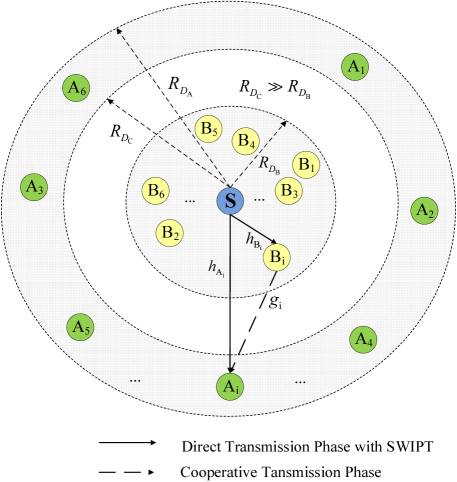
We consider a network with a single source SS\mathrm{S} (i.e., the base station (BS)) and two groups of randomly deployed users {Ai}subscriptAi\{\mathrm{A_{i}}\} and {Bi}subscriptBi\{\mathrm{B_{i}}\}. We assume that the users in group {Bi}subscriptBi\{\mathrm{B_{i}}\} are deployed within disc DBsubscript𝐷B{D_{\rm{B}}} with radius RDBsubscript𝑅subscript𝐷B{R_{{D_{\rm{B}}}}}. The far users {Ai}subscriptAi\{\mathrm{A_{i}}\} are deployed within ring DAsubscript𝐷A{D_{\rm{A}}} with radius RDCsubscript𝑅subscript𝐷C{R_{{D_{\rm{C}}}}} and RDAsubscript𝑅subscript𝐷A{R_{{D_{\rm{A}}}}}(assuming RDCRDBmuch-greater-thansubscript𝑅subscript𝐷Csubscript𝑅subscript𝐷B{R_{{D_{\rm{C}}}}}\gg{R_{{D_{\rm{B}}}}}), as shown in Fig. 1. Note that the BS is located at the origin of both the disc DBsubscript𝐷B{D_{\rm{B}}} and the ring DAsubscript𝐷A{D_{\rm{A}}}. The locations of the near and far users are modeled as homogeneous PPPs ΦκsubscriptΦ𝜅\Phi_{\kappa} (κ{A,B}𝜅AB\kappa\in\left\{{{\rm{A,B}}}\right\}) with densities λΦκsubscript𝜆subscriptΦ𝜅\lambda_{\Phi_{\kappa}}. Here the near users are uniformly distributed within the disc and the far users are uniformly distributed within the ring. The number of users in RDκsubscript𝑅subscript𝐷𝜅{R_{{D_{\kappa}}}}, denoted by Nκsubscript𝑁𝜅N_{\kappa}, follows a Poisson distribution Pr(Nκ=k)=(μκk/k!)eμκPrsubscript𝑁𝜅𝑘superscriptsubscript𝜇𝜅𝑘𝑘superscript𝑒subscript𝜇𝜅\Pr\left({N_{\kappa}=k}\right)=(\mu_{\kappa}^{k}/k!){e^{-{\mu_{\kappa}}}}, where μκsubscript𝜇𝜅{\mu_{\kappa}} is the mean measure, i.e., μA=π(RDA2RDC2)λΦAsubscript𝜇A𝜋superscriptsubscript𝑅subscript𝐷A2superscriptsubscript𝑅subscript𝐷C2subscript𝜆subscriptΦA{\mu_{\rm{A}}}=\pi\left({R_{{D_{\rm{A}}}}^{2}-R_{{D_{\rm{C}}}}^{2}}\right){\lambda_{{\Phi_{\rm{A}}}}} and μB=πRDB2λΦBsubscript𝜇B𝜋superscriptsubscript𝑅subscript𝐷B2subscript𝜆subscriptΦB{\mu_{\rm{B}}}=\pi R_{{D_{\rm{B}}}}^{2}{\lambda_{{\Phi_{\rm{B}}}}}. All channels are assumed to be quasi-static Rayleigh fading, where the channel coefficients are constant for each transmission block but vary independently between different blocks. In the proposed network, we consider that the users in {Bi}subscriptBi\{\mathrm{B_{i}}\} are energy harvesting relays that harvest energy from the BS and forward the information to {Ai}subscriptAi\{\mathrm{A_{i}}\} using the harvested energy as their transmit powers. The DF strategy is applied at {Bi}subscriptBi\{\mathrm{B_{i}}\} and the cooperative NOMA system consists of two phases, detailed in the following. In this work, without loss of generality, it is assumed that the two phases have the same transmission periods, the same as in [8, 10, 11]. It is worth pointing out that dynamic time allocation for the two phases may further improve the performance of the proposed cooperative NOMA scheme, but consideration of this issue is beyond the scope of the paper.
Refer to caption
Figure 1: An illustration of a aownlink SWIPT NOMA system with a base station S (blue circle). The spatial distributions of the near users (yellow circles) and the far users (green circles) follow homogeneous PPPs.

II-A Phase 1: Direct Transmission

Prior to transmission, the two users denoted by AisubscriptAi\mathrm{A_{i}} and BisubscriptBi\mathrm{B_{i}}, are selected to perform NOMA, where the selection criterion will be discussed in the next section. During the first phase, the BS sends two messages pi1xi1+pi2xi2subscript𝑝𝑖1subscript𝑥𝑖1subscript𝑝𝑖2subscript𝑥𝑖2{p_{i1}}{x_{i1}}+{p_{i2}}{x_{i2}} to two selected users AisubscriptAi\mathrm{A_{i}} and BisubscriptBi\mathrm{B_{i}} based on NOMA [3], where pi1subscript𝑝𝑖1p_{i1} and pi2subscript𝑝𝑖2p_{i2} are the power allocation coefficients and xi1subscript𝑥𝑖1x_{i1} and xi2subscript𝑥𝑖2x_{i2} are the messages of AisubscriptAi\mathrm{A_{i}} and BisubscriptBi\mathrm{B_{i}}, respectively. The observation at AisubscriptAi\mathrm{A_{i}} is given by

yAi,1=PSk{1,2}pikxikhAi1+dAiα+nAi,1,subscript𝑦subscriptAi1subscript𝑃Ssubscript𝑘12subscript𝑝𝑖𝑘subscript𝑥𝑖𝑘subscriptsubscriptAi1superscriptsubscript𝑑subscriptAi𝛼subscript𝑛subscriptAi1\displaystyle{y_{\mathrm{A_{i}},1}}=\sqrt{{P_{\rm{S}}}}\sum\limits_{k\in\left\{{1,2}\right\}}{{p_{ik}}{x_{ik}}}\frac{{{h_{\mathrm{A_{i}}}}}}{\sqrt{1+d_{\rm{A_{i}}}^{\alpha}}}+{n_{\mathrm{A_{i}},1}}, (1)

where PSsubscript𝑃S{P_{\rm{S}}} is the transmit power at the BS, hAisubscriptsubscriptAih_{\mathrm{A_{i}}} models the small-scale Rayleigh fading from the BS to AisubscriptAi\mathrm{A_{i}} with hAi𝒞𝒩(0,1)similar-tosubscriptsubscriptAi𝒞𝒩01{h_{\mathrm{A_{i}}}}\sim\mathcal{CN}({0,1}), nAi,1subscript𝑛subscriptAi1n_{\mathrm{A_{i}},1} is additive Gaussian white noise (AWGN) at AisubscriptAi\mathrm{A_{i}} with variance σAi2superscriptsubscript𝜎subscriptAi2\sigma_{\mathrm{A_{i}}}^{2}, dAisubscript𝑑subscriptAi{d_{\mathrm{A_{i}}}} is the distance between BS and AisubscriptAi\mathrm{A_{i}}, and α𝛼\alpha is the path loss exponent.

Without loss of generality, we assume that |pi1|2>|pi2|2superscriptsubscript𝑝𝑖12superscriptsubscript𝑝𝑖22{\left|{{p_{i1}}}\right|^{2}}>{\left|{{p_{i2}}}\right|^{2}} with |pi1|2+|pi2|2=1superscriptsubscript𝑝𝑖12superscriptsubscript𝑝𝑖221{\left|{{p_{i1}}}\right|^{2}}+{\left|{{p_{i2}}}\right|^{2}}=1. The received signal to interference and noise ratio (SINR) at AisubscriptAi\mathrm{A_{i}} to detect xi1subscript𝑥𝑖1x_{i1} is given by

γS,Aixi1=ρ|hAi|2|pi1|2ρ|pi2|2|hAi|2+1+dAiα,superscriptsubscript𝛾SsubscriptAisubscript𝑥𝑖1𝜌superscriptsubscriptsubscriptAi2superscriptsubscript𝑝𝑖12𝜌superscriptsubscript𝑝𝑖22superscriptsubscriptsubscriptAi21superscriptsubscript𝑑subscriptAi𝛼\displaystyle\gamma_{{\rm{S}},{{\rm{A}}_{\rm{i}}}}^{{x_{i1}}}=\frac{{\rho{{\left|{{h_{{{\rm{A}}_{\rm{i}}}}}}\right|}^{2}}{{\left|{{p_{i1}}}\right|}^{2}}}}{{\rho{{\left|{{p_{i2}}}\right|}^{2}}{{\left|{{h_{{{\rm{A}}_{\rm{i}}}}}}\right|}^{2}}+1+d_{{{\rm{A}}_{\rm{i}}}}^{\alpha}}}, (2)

where ρ=PSσ2𝜌subscript𝑃Ssuperscript𝜎2\rho=\frac{{P_{\rm{S}}}}{{{\sigma^{2}}}} is the transmit signal to noise radio (SNR) (assuming σAi2=σBi2=σ2superscriptsubscript𝜎subscriptAi2superscriptsubscript𝜎subscriptBi2superscript𝜎2\sigma_{\rm{A_{i}}}^{2}=\sigma_{\rm{B_{i}}}^{2}={\sigma^{2}}).

We consider that the near users have rechargeable storage ability [8] and power splitting [7] is applied to perform SWIPT. From the implementation point of view, this rechargeable storage unit can be a supercapacitor or a short-term high-efficiency battery [9]. The power splitting approach is applied as explained in the following: the observation at BisubscriptBi\mathrm{B_{i}} is divided into two parts. One part is used for information decoding by directing the observation flow to the detection circuit and the remaining part is used for energy harvesting to powers BisubscriptBi\mathrm{B_{i}} for helping AisubscriptAi\mathrm{A_{i}}. Thus,

yBi,1=PSk{1,2}pikxik1βihBi1+dBiα+nBi,1,subscript𝑦subscriptBi1subscript𝑃Ssubscript𝑘12subscript𝑝𝑖𝑘subscript𝑥𝑖𝑘1subscript𝛽𝑖subscriptsubscriptBi1superscriptsubscript𝑑subscriptBi𝛼subscript𝑛subscriptBi1\displaystyle{y_{\mathrm{B_{i}},1}}=\sqrt{{P_{\rm{S}}}}\sum\limits_{k\in\left\{{1,2}\right\}}{{p_{ik}}{x_{ik}}}\frac{{\sqrt{1-\beta_{i}}{h_{\mathrm{B_{i}}}}}}{\sqrt{1+d_{\rm{B_{i}}}^{\alpha}}}+{n_{\mathrm{B_{i}},1}}, (3)

where βisubscript𝛽𝑖\beta_{i} is the power splitting coefficient which is detailed in (7), hBisubscriptsubscriptBih_{\mathrm{B_{i}}} models the small-scale Rayleigh fading from the BS to BisubscriptBi\mathrm{B_{i}} with hBi𝒞𝒩(0,1)similar-tosubscriptsubscriptBi𝒞𝒩01{h_{\mathrm{B_{i}}}}\sim\mathcal{CN}({0,1}), nBisubscript𝑛subscriptBin_{\mathrm{B_{i}}} is AWGN at nBi,1subscript𝑛subscriptBi1{n_{\mathrm{B_{i}},1}} with variance σBi2superscriptsubscript𝜎subscriptBi2\sigma_{\mathrm{B_{i}}}^{2}, and dBisubscript𝑑subscriptBi{d_{\mathrm{B_{i}}}} is the distance between the BS and BisubscriptBi\mathrm{B_{i}}. We use the bounded path loss model to ensure that the path loss is always larger than one even for small distances [10].

Applying NOMA, successive interference cancellation (SIC)[12] is carried out at BisubscriptBi\mathrm{B_{i}}. Particularly, BisubscriptBi\mathrm{B_{i}} first decodes the message of AisubscriptAi\mathrm{A_{i}}, then subtracts this component from the received signal to detect its own information. Therefore, the received SINR at BisubscriptBi\mathrm{B_{i}} to detect xi1subscript𝑥𝑖1x_{i1} of AisubscriptAi\mathrm{A_{i}} is given by

γS,Bixi1=ρ|hBi|2|pi1|2(1βi)ρ|hBi|2|pi2|2(1βi)+1+dBiα.superscriptsubscript𝛾SsubscriptBisubscript𝑥𝑖1𝜌superscriptsubscriptsubscriptBi2superscriptsubscript𝑝𝑖121subscript𝛽𝑖𝜌superscriptsubscriptsubscriptBi2superscriptsubscript𝑝𝑖221subscript𝛽𝑖1superscriptsubscript𝑑subscriptBi𝛼\displaystyle\gamma_{{\rm{S}},{{\rm{B}}_{\rm{i}}}}^{{x_{i1}}}=\frac{{\rho{{\left|{{h_{{{\rm{B}}_{\rm{i}}}}}}\right|}^{2}}{{\left|{{p_{i1}}}\right|}^{2}}\left({1-{\beta_{i}}}\right)}}{{\rho{{\left|{{h_{{{\rm{B}}_{\rm{i}}}}}}\right|}^{2}}{{\left|{{p_{i2}}}\right|}^{2}}\left({1-{\beta_{i}}}\right)+1+d_{{{\rm{B}}_{\rm{i}}}}^{\alpha}}}. (4)

The received SNR at BisubscriptBi\mathrm{B_{i}} to detect xi2subscript𝑥𝑖2x_{i2} of BisubscriptBi\mathrm{B_{i}} is given by

γS,Bixi2=ρ|hBi|2|pi2|2(1βi)1+dBiα.superscriptsubscript𝛾SsubscriptBisubscript𝑥𝑖2𝜌superscriptsubscriptsubscriptBi2superscriptsubscript𝑝𝑖221subscript𝛽𝑖1superscriptsubscript𝑑subscriptBi𝛼\displaystyle\gamma_{{\rm{S}},{{\rm{B}}_{\rm{i}}}}^{{x_{i2}}}=\frac{{\rho{{\left|{{h_{{{\rm{B}}_{\rm{i}}}}}}\right|}^{2}}{{\left|{{p_{i2}}}\right|}^{2}}\left({1-{\beta_{i}}}\right)}}{{1+d_{{{\rm{B}}_{\rm{i}}}}^{\alpha}}}. (5)

The power splitting coefficient βisubscript𝛽𝑖\beta_{i} is used to determine the amount of harvested energy. Based on (4), the data rate supported by the channel from the BS to BisubscriptBi\mathrm{B_{i}} for decoding xi1subscript𝑥𝑖1x_{i1} is given by

Rxi1=12log(1+ρ|hBi|2|pi1|2(1βi)ρ|hBi|2|pi2|2(1βi)+1+dBiα).subscript𝑅subscript𝑥𝑖1121𝜌superscriptsubscriptsubscriptBi2superscriptsubscript𝑝𝑖121subscript𝛽𝑖𝜌superscriptsubscriptsubscriptBi2superscriptsubscript𝑝𝑖221subscript𝛽𝑖1superscriptsubscript𝑑subscriptBi𝛼\displaystyle{R_{{x_{i1}}}}=\frac{1}{2}\log\left({1+\frac{{\rho{{\left|{{h_{{{\rm{B}}_{\rm{i}}}}}}\right|}^{2}}{{\left|{{p_{i1}}}\right|}^{2}}\left({1-{\beta_{i}}}\right)}}{{\rho{{\left|{{h_{{{\rm{B}}_{\rm{i}}}}}}\right|}^{2}}{{\left|{{p_{i2}}}\right|}^{2}}\left({1-{\beta_{i}}}\right)+1+d_{{{\rm{B}}_{\rm{i}}}}^{\alpha}}}}\right). (6)

We assume that the energy required to receive/process information is negligible compared to the energy required for information transmission [8]. In this work, we apply the dynamic power splitting protocol which means that the power splitting coefficient βisubscript𝛽𝑖{\beta_{i}} is a variable and opportunistically tuned to support the relay transmission. Our aim is to first guarantee the detection of the message of the far NOMA user, AisubscriptAi\mathrm{A_{i}}, at the near NOMA user BisubscriptBi\mathrm{B_{i}}, then BisubscriptBi\mathrm{B_{i}} can harvest the remaining energy. In this case, based on (6), in order to ensure that BisubscriptBi\mathrm{B_{i}} can successfully decode the information of AisubscriptAi\mathrm{A_{i}}, we have a rate, i.e., R1=Rxi1subscript𝑅1subscript𝑅subscript𝑥𝑖1R_{1}=R_{x_{i1}}. Therefore, the power splitting coefficient is set as follows:

βi=max{0,1τ1(1+dBiα)ρ(|pi1|2τ1|pi2|2)|hBi|2},subscript𝛽𝑖01subscript𝜏11superscriptsubscript𝑑subscriptBi𝛼𝜌superscriptsubscript𝑝𝑖12subscript𝜏1superscriptsubscript𝑝𝑖22superscriptsubscriptsubscriptBi2\displaystyle{\beta_{i}}=\max\left\{{0,1-\frac{{{\tau_{1}}\left({1+d_{{{\rm{B}}_{\rm{i}}}}^{\alpha}}\right)}}{{\rho\left({{{\left|{{p_{i1}}}\right|}^{2}}-{\tau_{1}}{{\left|{{p_{i2}}}\right|}^{2}}}\right){{\left|{{h_{{{\rm{B}}_{\rm{i}}}}}}\right|}^{2}}}}}\right\}, (7)

where τ1=22R11subscript𝜏1superscript22subscript𝑅11{\tau_{1}}={2^{2{R_{1}}}}-1. Here βi=0subscript𝛽𝑖0\beta_{i}=0 means that all the energy is used for information decoding and no energy remains for energy harvesting.

Based on (3), the energy harvested at BisubscriptBi\mathrm{B_{i}} is given by

EBi=TηPSβi|hBi|22(1+dBiα),subscript𝐸subscriptBi𝑇𝜂subscript𝑃Ssubscript𝛽𝑖superscriptsubscriptsubscriptBi221superscriptsubscript𝑑subscriptBi𝛼\displaystyle{E_{\rm{B_{i}}}}=\frac{{T\eta{P_{\rm{S}}}\beta_{i}{{\left|{{h_{{{\rm{B}}_{\rm{i}}}}}}\right|}^{2}}}}{{2\left({1+d_{{{\rm{B}}_{\rm{i}}}}^{\alpha}}\right)}}, (8)

where T𝑇T is the time period for the entire transmission including the direct transmission phase and the cooperative transmission phase, and η𝜂\eta is the energy harvesting coefficient. We assume that the two phases have the same transmission period, and therefore, the transmit power at BisubscriptBi\mathrm{B_{i}} can be expressed as follows:

Pt=ηPSβi|hBi|21+dBiα.subscript𝑃𝑡𝜂subscript𝑃Ssubscript𝛽𝑖superscriptsubscriptsubscriptBi21superscriptsubscript𝑑subscriptBi𝛼\displaystyle{P_{t}}=\frac{{\eta{P_{\rm{S}}}\beta_{i}{{\left|{{h_{{{\rm{B}}_{\rm{i}}}}}}\right|}^{2}}}}{{1+d_{{{\rm{B}}_{\rm{i}}}}^{\alpha}}}. (9)

II-B Phase 2: Cooperative Transmission

During this phase, BisubscriptBi\mathrm{B_{i}} forwards xi1subscript𝑥𝑖1x_{i1} to AisubscriptAi\mathrm{A_{i}} by using the harvested energy during the direct transmission phase. In this case, AisubscriptAi\mathrm{A_{i}} observes

yAi,2=Ptxi1gi1+dCiα+nAi,2,subscript𝑦subscriptAi2subscript𝑃𝑡subscript𝑥𝑖1subscript𝑔i1superscriptsubscript𝑑subscriptCi𝛼subscript𝑛subscriptAi2\displaystyle{y_{{{\rm{A}}_{\rm{i}}},2}}=\frac{{\sqrt{{P_{t}}}{x_{i1}}{g_{\rm{i}}}}}{{\sqrt{1+d_{{{\rm{C}}_{\rm{i}}}}^{\alpha}}}}+{n_{{{\rm{A}}_{\rm{i}}},2}}, (10)

where gisubscript𝑔ig_{\mathrm{i}} models the small-scale Rayleigh fading from BisubscriptBi\mathrm{B_{i}} to AisubscriptAi\mathrm{A_{i}} with gi𝒞𝒩(0,1)similar-tosubscript𝑔i𝒞𝒩01g_{\mathrm{i}}\sim\mathcal{CN}({0,1}), nAi,2subscript𝑛subscriptAi2{n_{\rm{A_{i}},2}} is AWGN at AisubscriptAi\mathrm{A_{i}} with variance σAi2superscriptsubscript𝜎subscriptAi2\sigma_{\mathrm{A_{i}}}^{2}, dCi=dAi2+dBi22dAidBicos(θi)subscript𝑑subscriptCisuperscriptsubscript𝑑subscriptAi2superscriptsubscript𝑑subscriptBi22subscript𝑑subscriptAisubscript𝑑subscriptBisubscript𝜃𝑖{d_{{{\rm{C}}_{\rm{i}}}}}=\sqrt{d_{{{\rm{A}}_{\rm{i}}}}^{2}+d_{{{\rm{B}}_{\rm{i}}}}^{2}-2{d_{{{\rm{A}}_{\rm{i}}}}}{d_{{{\rm{B}}_{\rm{i}}}}}\cos\left({{\theta_{i}}}\right)} is the distance between BisubscriptBi\mathrm{B_{i}} and AisubscriptAi\mathrm{A_{i}}, and θisubscript𝜃𝑖{\theta_{i}} denotes the angle AiSBisubscriptAisubscriptSBi\angle{{\rm{A}}_{\rm{i}}}{\rm{S}}{{\rm{B}}_{\rm{i}}}.

Based on (9) and (10), the received SNR for AisubscriptAi\mathrm{A_{i}} to detect xi1subscript𝑥𝑖1x_{i1} forwarded from BisubscriptBi\mathrm{B_{i}} is given by

γAi,Bixi1=Pt|gi|2(1+dCiα)σ2=ηρβi|hBi|2|gi|2(1+dCiα)(1+dBiα).superscriptsubscript𝛾subscriptAisubscriptBisubscript𝑥𝑖1subscript𝑃𝑡superscriptsubscript𝑔𝑖21superscriptsubscript𝑑subscriptCi𝛼superscript𝜎2𝜂𝜌subscript𝛽𝑖superscriptsubscriptsubscriptBi2superscriptsubscript𝑔𝑖21superscriptsubscript𝑑subscriptCi𝛼1superscriptsubscript𝑑subscriptBi𝛼\displaystyle\gamma_{{{\rm{A}}_{\rm{i}}},{{\rm{B}}_{\rm{i}}}}^{{x_{i1}}}=\frac{{{P_{t}}{{\left|{{g_{i}}}\right|}^{2}}}}{{\left({1+d_{{{\rm{C}}_{\rm{i}}}}^{\alpha}}\right){\sigma^{2}}}}=\frac{{\eta\rho{\beta_{i}}{{\left|{{h_{{{\rm{B}}_{\rm{i}}}}}}\right|}^{2}}{{\left|{{g_{i}}}\right|}^{2}}}}{{\left({1+d_{{{\rm{C}}_{\rm{i}}}}^{\alpha}}\right)\left({1+d_{{{\rm{B}}_{\rm{i}}}}^{\alpha}}\right)}}. (11)

At the end of this phase, AisubscriptAi\mathrm{A_{i}} combines the signals from the BS and BisubscriptBi\mathrm{B_{i}} using maximal-ratio combining (MRC). Combining the SNR of the direct transmission phase (2) and the SINR of the cooperative transmission phase (11), we obtain the received SINR at AisubscriptAi\mathrm{A_{i}} as follows:

γAi,MRCxi1=ρ|hAi|2|pi1|2ρ|hAi|2|pi2|2+1+dAiα+ηρβi|hBi|2|gi|2(1+dBiα)(1+dCiα).superscriptsubscript𝛾subscriptAiMRCsubscript𝑥𝑖1𝜌superscriptsubscriptsubscriptAi2superscriptsubscript𝑝𝑖12𝜌superscriptsubscriptsubscriptAi2superscriptsubscript𝑝𝑖221superscriptsubscript𝑑subscriptAi𝛼𝜂𝜌subscript𝛽𝑖superscriptsubscriptsubscriptBi2superscriptsubscript𝑔𝑖21superscriptsubscript𝑑subscriptBi𝛼1superscriptsubscript𝑑subscriptCi𝛼\displaystyle\gamma_{{{\rm{A}}_{\rm{i}}},{\rm{MRC}}}^{{x_{i1}}}=\frac{{\rho{{\left|{{h_{{{\rm{A}}_{\rm{i}}}}}}\right|}^{2}}{{\left|{{p_{i1}}}\right|}^{2}}}}{{\rho{{\left|{{h_{{{\rm{A}}_{\rm{i}}}}}}\right|}^{2}}{{\left|{{p_{i2}}}\right|}^{2}}+1+d_{{{\rm{A}}_{\rm{i}}}}^{\alpha}}}+\frac{{\eta\rho{\beta_{i}}{{\left|{{h_{{{\rm{B}}_{\rm{i}}}}}}\right|}^{2}}{{\left|{{g_{i}}}\right|}^{2}}}}{{\left({1+d_{{{\rm{B}}_{\rm{i}}}}^{\alpha}}\right)\left({1+d_{{{\rm{C}}_{\rm{i}}}}^{\alpha}}\right)}}. (12)

III Non-Orthogonal Multiple Access with User Selection

In this section, the performance of three user selection schemes are characterized in the following.

III-A RNRF Selection Scheme

In this scheme, the BS randomly selects a near user BisubscriptBi\rm{B_{i}} and a far user AisubscriptAi\rm{A_{i}}. This selection scheme provides a fair opportunity for each user to access the source with the NOMA protocol. The advantage of this user selection scheme is that it does not require the knowledge of instantaneous channel state information (CSI). To make meaningful conclusions, in the rest of the paper, we only focus on βi>0subscript𝛽𝑖0{\beta_{i}}>0 and the number of near users and far users satisfy NB1,NA1formulae-sequencesubscript𝑁𝐵1subscript𝑁𝐴1{N_{B}}\geq 1,{N_{A}}\geq 1.

III-A1 Outage Probability of the Near Users of RNRF

In the NOMA protocol, an outage of BisubscriptBi\mathrm{B_{i}} can occur for two reasons. The first is that BisubscriptBi\mathrm{B_{i}} cannot detect xi1subscript𝑥𝑖1x_{i1}. The second is that BisubscriptBi\mathrm{B_{i}} can detect xi1subscript𝑥𝑖1x_{i1} but cannot detect xi2subscript𝑥𝑖2x_{i2}. To guarantee that the NOMA protocol can be implemented, the condition |pi1|2|pi2|2τ1>0superscriptsubscript𝑝𝑖12superscriptsubscript𝑝𝑖22subscript𝜏10{\left|{{p_{i1}}}\right|^{2}}-{\left|{{p_{i2}}}\right|^{2}}{\tau_{1}}>0 should be satisfied [3]. Based on this, the outage probability of BisubscriptBi\mathrm{B_{i}} can be expressed as follows:

PBi=Pr(ρ|hBi|2|pi1|2ρ|hBi|2|pi2|2+1+dBiα<τ1)subscript𝑃subscriptBiPr𝜌superscriptsubscriptsubscriptBi2superscriptsubscript𝑝𝑖12𝜌superscriptsubscriptsubscriptBi2superscriptsubscript𝑝𝑖221superscriptsubscript𝑑subscriptBi𝛼subscript𝜏1\displaystyle{P_{{{\rm{B}}_{\rm{i}}}}}=\Pr\left({\frac{{\rho{{\left|{{h_{{{\rm{B}}_{\rm{i}}}}}}\right|}^{2}}{{\left|{{p_{i1}}}\right|}^{2}}}}{{\rho{{\left|{{h_{{{\rm{B}}_{\rm{i}}}}}}\right|}^{2}}{{\left|{{p_{i2}}}\right|}^{2}}+1+d_{{{\rm{B}}_{\rm{i}}}}^{\alpha}}}<{\tau_{1}}}\right)
+Pr(ρ|hBi|2|pi1|2ρ|hBi|2|pi2|2+1+dBiα>τ1,γS,Bixi2<τ2),Pr𝜌superscriptsubscriptsubscriptBi2superscriptsubscript𝑝𝑖12𝜌superscriptsubscriptsubscriptBi2superscriptsubscript𝑝𝑖221superscriptsubscript𝑑subscriptBi𝛼subscript𝜏1superscriptsubscript𝛾SsubscriptBisubscript𝑥𝑖2subscript𝜏2\displaystyle+\Pr\left({\frac{{\rho{{\left|{{h_{{{\rm{B}}_{\rm{i}}}}}}\right|}^{2}}{{\left|{{p_{i1}}}\right|}^{2}}}}{{\rho{{\left|{{h_{{{\rm{B}}_{\rm{i}}}}}}\right|}^{2}}{{\left|{{p_{i2}}}\right|}^{2}}+1+d_{{{\rm{B}}_{\rm{i}}}}^{\alpha}}}>{\tau_{1}},\gamma_{{\rm{S}},{{\rm{B}}_{\rm{i}}}}^{{x_{i2}}}<{\tau_{2}}}\right), (13)

where τ2=22R21subscript𝜏2superscript22subscript𝑅21{\tau_{2}}={2^{2{R_{2}}}}-1 with R2subscript𝑅2R_{2} being the target rate at which BisubscriptBi\mathrm{B_{i}} can detect xi2subscript𝑥𝑖2x_{i2}.

The following theorem provides the outage probability of the near users in RNRF for an arbitrary choice of α𝛼\alpha.

Theorem 1

Conditioned on the PPPs, the outage probability of the near users BisubscriptBi\mathrm{B_{i}} can be approximated as follows:

PBi12n=1NωN1ϕn2(1ecnεAi)(ϕn+1),subscript𝑃subscriptBi12superscriptsubscript𝑛1𝑁subscript𝜔𝑁1superscriptsubscriptitalic-ϕ𝑛21superscript𝑒subscript𝑐𝑛subscript𝜀subscriptA𝑖subscriptitalic-ϕ𝑛1\displaystyle{P_{{{\rm{B}}_{\rm{i}}}}}\approx\frac{1}{2}\sum\limits_{n=1}^{N}{{\omega_{N}}\sqrt{1-{\phi_{n}}^{2}}\left({1-{e^{-{c_{n}}{\varepsilon_{{{\rm{A}}_{i}}}}}}}\right)\left({{\phi_{n}}+1}\right)}, (14)

if εAiεBisubscript𝜀subscriptA𝑖subscript𝜀subscriptB𝑖{\varepsilon_{{{\rm{A}}_{i}}}}\geq{\varepsilon_{{{\rm{B}}_{i}}}}, otherwise PBi=1subscript𝑃subscriptBi1{P_{{{\rm{B}}_{\rm{i}}}}}=1, where εAi=τ1ρ(|pi1|2|pi2|2τ1)subscript𝜀subscriptA𝑖subscript𝜏1𝜌superscriptsubscript𝑝𝑖12superscriptsubscript𝑝𝑖22subscript𝜏1{\varepsilon_{{{\rm{A}}_{i}}}}=\frac{{{\tau_{1}}}}{{\rho\left({{{\left|{{p_{i1}}}\right|}^{2}}-{{\left|{{p_{i2}}}\right|}^{2}}{\tau_{1}}}\right)}} and εBi=τ2ρ|pi2|2subscript𝜀subscriptB𝑖subscript𝜏2𝜌superscriptsubscript𝑝𝑖22{\varepsilon_{{{\rm{B}}_{i}}}}=\frac{{{\tau_{2}}}}{{\rho{{\left|{{p_{i2}}}\right|}^{2}}}}, N𝑁N is a parameter to ensure a complexity-accuracy tradeoff, cn=1+(RDB2(ϕn+1))αsubscript𝑐𝑛1superscriptsubscript𝑅subscript𝐷B2subscriptitalic-ϕ𝑛1𝛼{c_{n}}=1+{\left({\frac{{{R_{{D_{\rm{B}}}}}}}{2}\left({{\phi_{n}}+1}\right)}\right)^{\alpha}}, ωN=πNsubscript𝜔𝑁𝜋𝑁{\omega_{N}}=\frac{\pi}{N}, and ϕn=cos(2n12Nπ)subscriptitalic-ϕ𝑛2𝑛12𝑁𝜋{\phi_{n}}=\cos\left({\frac{{2n-1}}{{2N}}\pi}\right).

Proof:

Define Xi=|hAi|21+dAiα,Yi=|hBi|21+dBiαformulae-sequencesubscript𝑋𝑖superscriptsubscriptsubscriptAi21superscriptsubscript𝑑subscriptAi𝛼subscript𝑌𝑖superscriptsubscriptsubscriptBi21superscriptsubscript𝑑subscriptBi𝛼{X_{i}}=\frac{{{{\left|{{h_{{{\rm{A}}_{\rm{i}}}}}}\right|}^{2}}}}{{1+d_{{{\rm{A}}_{\rm{i}}}}^{\alpha}}},{Y_{i}}=\frac{{{{\left|{{h_{{{\rm{B}}_{\rm{i}}}}}}\right|}^{2}}}}{{1+d_{{{\rm{B}}_{\rm{i}}}}^{\alpha}}}, and Zi=|gi|21+dCiαsubscript𝑍𝑖superscriptsubscript𝑔𝑖21superscriptsubscript𝑑subscriptCi𝛼{Z_{i}}=\frac{{{{\left|{{g_{i}}}\right|}^{2}}}}{{1+d_{{{\rm{C}}_{\rm{i}}}}^{\alpha}}}. Substituting (4) and (5) into (III-A1), the outage probability of the near users is given by

PBi=Pr(Yi<εAi)+Pr(Yi>εAi,εAi<εBi).subscript𝑃subscriptBiPrsubscript𝑌𝑖subscript𝜀subscriptA𝑖Prsubscript𝑌𝑖subscript𝜀subscriptA𝑖subscript𝜀subscriptA𝑖subscript𝜀subscriptB𝑖\displaystyle{P_{{{\rm{B}}_{\rm{i}}}}}=\Pr\left({{Y_{i}}<{\varepsilon_{{{\rm{A}}_{i}}}}}\right)+\Pr\left({{Y_{i}}>{\varepsilon_{{{\rm{A}}_{i}}}},{\varepsilon_{{{\rm{A}}_{i}}}}<{\varepsilon_{{{\rm{B}}_{i}}}}}\right). (15)

If εAi<εBisubscript𝜀subscriptA𝑖subscript𝜀subscriptB𝑖{\varepsilon_{{{\rm{A}}_{i}}}}<{\varepsilon_{{{\rm{B}}_{i}}}}, the outage probability at the near users is always one.

For the case εAiεBisubscript𝜀subscriptA𝑖subscript𝜀subscriptB𝑖{\varepsilon_{{{\rm{A}}_{i}}}}\geq{\varepsilon_{{{\rm{B}}_{i}}}}, note that the users are deployed in DBsubscript𝐷B{D_{\rm{B}}} and DAsubscript𝐷A{D_{\rm{A}}} according to homogeneous PPPs. Therefore, the NOMA users are modeled as independently and identically distributed (i.i.d.) points in DBsubscript𝐷B{D_{\rm{B}}} and DAsubscript𝐷A{D_{\rm{A}}}, denoted by Wκisubscript𝑊subscript𝜅𝑖{W_{{\kappa_{i}}}} (κ{A,B})𝜅AB\left({\kappa\in\left\{{\mathrm{A},\mathrm{B}}\right\}}\right), which contain the location information about AisubscriptAi\mathrm{A_{i}} and BisubscriptBi\mathrm{B_{i}}, respectively. The probability density functions (PDFs) of WAisubscript𝑊subscriptAi{W_{{\mathrm{A_{i}}}}} and WBisubscript𝑊subscriptBi{W_{{\mathrm{B_{i}}}}} are given by

fWBi(ωBi)=λΦBμRDB=1πRDB2,subscript𝑓subscript𝑊subscriptBisubscript𝜔subscriptBisubscript𝜆subscriptΦBsubscript𝜇subscript𝑅subscript𝐷B1𝜋superscriptsubscript𝑅subscript𝐷B2\displaystyle{f_{{W_{{{\rm{B}}_{\rm{i}}}}}}}\left({{\omega_{{{\rm{B}}_{\rm{i}}}}}}\right)=\frac{{{\lambda_{{\Phi_{\rm{B}}}}}}}{{{\mu_{{R_{{D_{\rm{B}}}}}}}}}=\frac{1}{{\pi R_{{D_{\rm{B}}}}^{2}}}, (16)

and

fWAi(ωAi)=λΦAμRDA=1π(RDA2RDC2),subscript𝑓subscript𝑊subscriptAisubscript𝜔subscriptAisubscript𝜆subscriptΦAsubscript𝜇subscript𝑅subscript𝐷A1𝜋superscriptsubscript𝑅subscript𝐷A2superscriptsubscript𝑅subscript𝐷C2\displaystyle{f_{{W_{{{\rm{A}}_{\rm{i}}}}}}}\left({{\omega_{{{\rm{A}}_{\rm{i}}}}}}\right)=\frac{{{\lambda_{{\Phi_{\rm{A}}}}}}}{{{\mu_{{R_{{D_{\rm{A}}}}}}}}}=\frac{1}{{\pi\left({R_{{D_{\rm{A}}}}^{2}-R_{{D_{\rm{C}}}}^{2}}\right)}}, (17)

respectively.

Therefore, for the case εAiεBisubscript𝜀subscriptA𝑖subscript𝜀subscriptB𝑖{\varepsilon_{{{\rm{A}}_{i}}}}\geq{\varepsilon_{{{\rm{B}}_{i}}}}, the cumulative distribution function (CDF) of Yisubscript𝑌𝑖{Y_{i}} is given by

FYi(ε)=subscript𝐹subscript𝑌𝑖𝜀absent\displaystyle{F_{Y_{i}}}\left(\varepsilon\right)= DB(1e(1+dBiα)ε)fWBi(ωBi)𝑑ωBisubscriptsubscript𝐷B1superscript𝑒1superscriptsubscript𝑑subscriptBi𝛼𝜀subscript𝑓subscript𝑊subscriptBisubscript𝜔subscriptBidifferential-dsubscript𝜔subscriptBi\displaystyle\int\limits_{D_{{\rm{B}}}}{\left({1-{e^{-\left({1+d_{{{\rm{B}}_{\rm{i}}}}^{\alpha}}\right)\varepsilon}}}\right){f_{{W_{{{\rm{B}}_{\rm{i}}}}}}}\left({{\omega_{{{\rm{B}}_{\rm{i}}}}}}\right)d{\omega_{{{\rm{B}}_{\rm{i}}}}}}
=\displaystyle= 2RDB20RDB(1e(1+rα)ε)r𝑑r.2superscriptsubscript𝑅subscript𝐷B2superscriptsubscript0subscript𝑅subscript𝐷B1superscript𝑒1superscript𝑟𝛼𝜀𝑟differential-d𝑟\displaystyle\frac{2}{{R_{{D_{\rm{B}}}}^{2}}}\int_{0}^{{R_{{D_{\rm{B}}}}}}{\left({1-{e^{-\left({1+{r^{\alpha}}}\right)\varepsilon}}}\right)rdr}. (18)

For many communication scenarios α>2𝛼2\alpha>2, and it is challenging to obtain exact closed-from expressions for the above. In this case, we can use Gaussian-Chebyshev quadrature [13] to find the approximation of (1) as follows:

FYi(ε)12n=1NωN1ϕn2(1ecnε)(ϕn+1).subscript𝐹subscript𝑌𝑖𝜀12superscriptsubscript𝑛1𝑁subscript𝜔𝑁1superscriptsubscriptitalic-ϕ𝑛21superscript𝑒subscript𝑐𝑛𝜀subscriptitalic-ϕ𝑛1\displaystyle{F_{Y_{i}}}\left(\varepsilon\right)\approx\frac{1}{2}\sum\limits_{n=1}^{N}{{\omega_{N}}\sqrt{1-{\phi_{n}}^{2}}\left({1-{e^{-{c_{n}}\varepsilon}}}\right)\left({{\phi_{n}}+1}\right)}. (19)

Applying εAiεsubscript𝜀subscriptA𝑖𝜀{\varepsilon_{{{\rm{A}}_{i}}}}\to\varepsilon into (19), (14) is obtained, and the proof of the theorem is completed. ∎

Corollary 1

For the special case α=2𝛼2\alpha=2, the outage probability of BisubscriptBi\mathrm{B_{i}} can be obtained as follows:

PBi|α=2=1eεAiRDB2εAi+e(1+RDB2)εAiRDB2εAi,evaluated-atsubscript𝑃subscriptBi𝛼21superscript𝑒subscript𝜀subscriptA𝑖superscriptsubscript𝑅subscript𝐷B2subscript𝜀subscriptA𝑖superscript𝑒1superscriptsubscript𝑅subscript𝐷B2subscript𝜀subscriptA𝑖superscriptsubscript𝑅subscript𝐷B2subscript𝜀subscriptA𝑖\displaystyle{\left.{{P_{{{\rm{B}}_{\rm{i}}}}}}\right|_{\alpha=2}}=1-\frac{{{e^{-{\varepsilon_{{{\rm{A}}_{i}}}}}}}}{{R_{{D_{\rm{B}}}}^{2}{\varepsilon_{{{\rm{A}}_{i}}}}}}+\frac{{{e^{-\left({1+R_{{D_{\rm{B}}}}^{2}}\right){\varepsilon_{{{\rm{A}}_{i}}}}}}}}{{R_{{D_{\rm{B}}}}^{2}{\varepsilon_{{{\rm{A}}_{i}}}}}}, (20)

if εAiεBisubscript𝜀subscriptA𝑖subscript𝜀subscriptB𝑖{\varepsilon_{{{\rm{A}}_{i}}}}\geq{\varepsilon_{{{\rm{B}}_{i}}}}, otherwise PBi|α=2=1evaluated-atsubscript𝑃subscriptBi𝛼21{\left.{{P_{{{\rm{B}}_{\rm{i}}}}}}\right|_{\alpha=2}}=1.

Proof:

Based on (1), when α=2𝛼2\alpha=2 and after some manipulations, we can easily obtain

FYi(ε)|α=2=1eεRDB2ε+e(1+RDB2)εRDB2ε.evaluated-atsubscript𝐹subscript𝑌𝑖𝜀𝛼21superscript𝑒𝜀superscriptsubscript𝑅subscript𝐷B2𝜀superscript𝑒1superscriptsubscript𝑅subscript𝐷B2𝜀superscriptsubscript𝑅subscript𝐷B2𝜀\displaystyle{\left.{{F_{Y_{i}}}\left(\varepsilon\right)}\right|_{\alpha=2}}=1-\frac{{{e^{-\varepsilon}}}}{{R_{{D_{\rm{B}}}}^{2}\varepsilon}}+\frac{{{e^{-\left({1+R_{{D_{\rm{B}}}}^{2}}\right)\varepsilon}}}}{{R_{{D_{\rm{B}}}}^{2}\varepsilon}}. (21)

Applying εAiεsubscript𝜀subscriptA𝑖𝜀{\varepsilon_{{{\rm{A}}_{i}}}}\to\varepsilon into (21), (20) can be obtained. The proof is completed. ∎

III-A2 Outage Probability of the Far Users of RNRF

With the proposed cooperative SWIPT NOMA protocol, outage experienced by AisubscriptAi\mathrm{A_{i}} can occur in two situations. The first is when BisubscriptBi\mathrm{B_{i}} can detect xi1subscript𝑥𝑖1x_{i1} but the overall received SNR at AisubscriptAi\mathrm{A_{i}} cannot support the targeted rate. The second is when neither AisubscriptAi\mathrm{A_{i}} nor BisubscriptBi\mathrm{B_{i}} can detect xi1subscript𝑥𝑖1x_{i1}. Based on this, the outage probability can be expressed as follows:

PAi=subscript𝑃subscriptAiabsent\displaystyle{P_{{{\rm{A}}_{\rm{i}}}}}= Pr(γAi,MRCxi1<τ1,γS,Bixi1|βi=0>τ1)Prsuperscriptsubscript𝛾subscriptAiMRCsubscript𝑥𝑖1subscriptbrasubscript𝜏1superscriptsubscript𝛾SsubscriptBisubscript𝑥𝑖1subscript𝛽𝑖0subscript𝜏1\displaystyle\Pr\left({\gamma_{{{\rm{A}}_{\rm{i}}},{\rm{MRC}}}^{{x_{i1}}}<{\tau_{1}},{{\left.{\gamma_{{\rm{S}},{{\rm{B}}_{\rm{i}}}}^{{x_{i1}}}}\right|}_{{\beta_{i}}=0}}>{\tau_{1}}}\right)
+Pr(γS,Aixi1<τ1,γS,Bixi1|βi=0<τ1).Prsuperscriptsubscript𝛾SsubscriptAisubscript𝑥𝑖1subscriptbrasubscript𝜏1superscriptsubscript𝛾SsubscriptBisubscript𝑥𝑖1subscript𝛽𝑖0subscript𝜏1\displaystyle+\Pr\left({\gamma_{{\rm{S}},{{\rm{A}}_{\rm{i}}}}^{{x_{i1}}}<{\tau_{1}},{{\left.{\gamma_{{\rm{S}},{{\rm{B}}_{\rm{i}}}}^{{x_{i1}}}}\right|}_{{\beta_{i}}=0}}<{\tau_{1}}}\right). (22)

The following theorem provides the outage probability of the far users in RNRF for an arbitrary choice of α𝛼\alpha.

Theorem 2

Conditioned on the PPPs, and assuming RDCRDBmuch-greater-thansubscript𝑅subscript𝐷Csubscript𝑅subscript𝐷B{R_{{D_{\rm{C}}}}}\gg{R_{{D_{\rm{B}}}}}, the outage probability of AisubscriptAi\mathrm{A_{i}} can be approximated as follows:

PAiζ1n=1N(ϕn+1)1ϕn2cnk=1K1ψk2sk(1+skα)2subscript𝑃subscriptAisubscript𝜁1superscriptsubscript𝑛1𝑁subscriptitalic-ϕ𝑛11superscriptsubscriptitalic-ϕ𝑛2subscript𝑐𝑛superscriptsubscript𝑘1𝐾1superscriptsubscript𝜓𝑘2subscript𝑠𝑘superscript1superscriptsubscript𝑠𝑘𝛼2\displaystyle{P_{{{\rm{A_{i}}}}}}\approx\zeta_{1}\sum\limits_{n=1}^{N}{\left({{\phi_{n}}+1}\right)\sqrt{1-{\phi_{n}}^{2}}}{c_{n}}\sum\limits_{k=1}^{K}{\sqrt{1-\psi_{k}^{2}}{s_{k}}{{\left({1+s_{k}^{\alpha}}\right)}^{2}}}
×m=1M1φm2e(1+skα)tmχtm(lnχtm(1+skα)ηρcn+2c0)\displaystyle\times\sum\limits_{m=1}^{M}{\sqrt{1-\varphi_{m}^{2}}{e^{-\left({1+s_{k}^{\alpha}}\right){t_{m}}}}{\chi_{{t_{m}}}}\left({\ln\frac{{{\chi_{{t_{m}}}}\left({1+s_{k}^{\alpha}}\right)}}{{\eta\rho}}{c_{n}}+2{c_{0}}}\right)}
+a1n=1N1ϕn2cn(ϕn+1)k=1K1ψk2(1+skα)sk,subscript𝑎1superscriptsubscript𝑛1𝑁1superscriptsubscriptitalic-ϕ𝑛2subscript𝑐𝑛subscriptitalic-ϕ𝑛1superscriptsubscript𝑘1𝐾1superscriptsubscript𝜓𝑘21superscriptsubscript𝑠𝑘𝛼subscript𝑠𝑘\displaystyle+{a_{1}}\sum\limits_{n=1}^{N}{\sqrt{1-{\phi_{n}}^{2}}{c_{n}}\left({{\phi_{n}}+1}\right)}\sum\limits_{k=1}^{K}{\sqrt{1-{\psi_{k}}^{2}}(1+s_{k}^{\alpha}){s_{k}}}, (23)

where M𝑀M and K𝐾K are parameters to ensure a complexity-accuracy tradeoff, ζ1=εAiRDBiωNωKωM8(RDAi+RDCi)ηρ,χtm=τ1ρtm|pi1|2ρtm|pi2|2+1,tm=εAi2(φm+1),ωM=πM,φm=cos(2m12Mπ),sk=RDARDC2(ψk+1)+RDC,ωK=πK,ψk=cos(2k12Kπ)formulae-sequencesubscript𝜁1subscript𝜀subscriptA𝑖subscript𝑅subscript𝐷subscriptBisubscript𝜔𝑁subscript𝜔𝐾subscript𝜔𝑀8subscript𝑅subscript𝐷subscriptAisubscript𝑅subscript𝐷subscriptCi𝜂𝜌formulae-sequencesubscript𝜒subscript𝑡𝑚subscript𝜏1𝜌subscript𝑡𝑚superscriptsubscript𝑝𝑖12𝜌subscript𝑡𝑚superscriptsubscript𝑝𝑖221formulae-sequencesubscript𝑡𝑚subscript𝜀subscriptA𝑖2subscript𝜑𝑚1formulae-sequencesubscript𝜔𝑀𝜋𝑀formulae-sequencesubscript𝜑𝑚2𝑚12𝑀𝜋formulae-sequencesubscript𝑠𝑘subscript𝑅subscript𝐷Asubscript𝑅subscript𝐷C2subscript𝜓𝑘1subscript𝑅subscript𝐷Cformulae-sequencesubscript𝜔𝐾𝜋𝐾subscript𝜓𝑘2𝑘12𝐾𝜋{\zeta_{1}}=-\frac{{{\varepsilon_{{{\rm{A}}_{i}}}}{R_{{D_{{{\rm{B}}_{\rm{i}}}}}}}{\omega_{N}}{\omega_{K}}{\omega_{M}}}}{{8\left({{R_{{D_{{{\rm{A}}_{\rm{i}}}}}}}+{R_{{D_{{{\rm{C}}_{\rm{i}}}}}}}}\right)\eta\rho}},{\chi_{{t_{m}}}}={\tau_{1}}-\frac{{\rho{t_{m}}{{\left|{{p_{i1}}}\right|}^{2}}}}{{\rho{t_{m}}{{\left|{{p_{i2}}}\right|}^{2}}+1}},{t_{m}}=\frac{{{\varepsilon_{{{\rm{A}}_{i}}}}}}{2}\left({{\varphi_{m}}+1}\right),{\omega_{M}}=\frac{\pi}{M},{\varphi_{m}}=\cos\left({\frac{{2m-1}}{{2M}}\pi}\right),{s_{k}}=\frac{{{R_{{D_{\rm{A}}}}}-{R_{{D_{\rm{C}}}}}}}{2}\left({{\psi_{k}}+1}\right)+{R_{{D_{\rm{C}}}}},{\omega_{K}}=\frac{\pi}{K},{\psi_{k}}=\cos\left({\frac{{2k-1}}{{2K}}\pi}\right), c0=φ(1)2φ(2)2subscript𝑐0𝜑12𝜑22{c_{0}}=-\frac{{\varphi\left(1\right)}}{2}-\frac{{\varphi\left(2\right)}}{2}, and a1=ωKωNεA122(RDA+RDC)subscript𝑎1subscript𝜔𝐾subscript𝜔𝑁superscriptsubscript𝜀subscriptA122subscript𝑅subscript𝐷Asubscript𝑅subscript𝐷C{a_{1}}=\frac{{{\omega_{K}}{\omega_{N}}\varepsilon_{{{\rm{A}}_{1}}}^{2}}}{{2\left({{R_{{D_{\rm{A}}}}}+{R_{{D_{\rm{C}}}}}}\right)}}.

Proof:

See Appendix A. ∎

Corollary 2

For the special case α=2𝛼2\alpha=2, the outage probability of AisubscriptAi\mathrm{A_{i}} can be simplified as follows:

PAi|α=2evaluated-atsubscript𝑃subscriptAi𝛼2\displaystyle{\left.{{P_{{{\rm{A}}_{\rm{i}}}}}}\right|_{\alpha=2}} ζ2k=1K1ψk2sk(1+sk2)2m=1M1φm2absentsubscript𝜁2superscriptsubscript𝑘1𝐾1superscriptsubscript𝜓𝑘2subscript𝑠𝑘superscript1superscriptsubscript𝑠𝑘22superscriptsubscript𝑚1𝑀1superscriptsubscript𝜑𝑚2\displaystyle\approx{\zeta_{2}}\sum\limits_{k=1}^{K}{\sqrt{1-\psi_{k}^{2}}{s_{k}}{{\left({1+s_{k}^{2}}\right)}^{2}}}\sum\limits_{m=1}^{M}{\sqrt{1-\varphi_{m}^{2}}}
×χtme(1+sk2)tm(lnχtm(1+sk2)ηρcn+b0)absentsubscript𝜒subscript𝑡𝑚superscript𝑒1superscriptsubscript𝑠𝑘2subscript𝑡𝑚subscript𝜒subscript𝑡𝑚1superscriptsubscript𝑠𝑘2𝜂𝜌subscript𝑐𝑛subscript𝑏0\displaystyle\times{\chi_{{t_{m}}}}{e^{-\left({1+s_{k}^{2}}\right){t_{m}}}}\left({\ln\frac{{{\chi_{{t_{m}}}}\left({1+s_{k}^{2}}\right)}}{{\eta\rho}}{c_{n}}+{b_{0}}}\right)
+(1e(1+RDC2)εAiεAi(RDA2RDC2)+e(1+RDA2)εAiεAi(RDA2RDC2))1superscript𝑒1superscriptsubscript𝑅subscript𝐷C2subscript𝜀subscriptA𝑖subscript𝜀subscriptA𝑖superscriptsubscript𝑅subscript𝐷A2superscriptsubscript𝑅subscript𝐷C2superscript𝑒1superscriptsubscript𝑅subscript𝐷A2subscript𝜀subscriptA𝑖subscript𝜀subscriptA𝑖superscriptsubscript𝑅subscript𝐷A2superscriptsubscript𝑅subscript𝐷C2\displaystyle+\left({1-\frac{{{e^{-\left({1+R_{{D_{\rm{C}}}}^{2}}\right){\varepsilon_{{{\rm{A}}_{i}}}}}}}}{{{\varepsilon_{{{\rm{A}}_{i}}}}\left({R_{{D_{\rm{A}}}}^{2}-R_{{D_{\rm{C}}}}^{2}}\right)}}+\frac{{{e^{-\left({1+R_{{D_{\rm{A}}}}^{2}}\right){\varepsilon_{{{\rm{A}}_{i}}}}}}}}{{{\varepsilon_{{{\rm{A}}_{i}}}}\left({R_{{D_{\rm{A}}}}^{2}-R_{{D_{\rm{C}}}}^{2}}\right)}}}\right)
×(1eεAiRDB2εAi+e(1+RDB2)εAiRDB2εAi),absent1superscript𝑒subscript𝜀subscriptA𝑖superscriptsubscript𝑅subscript𝐷B2subscript𝜀subscriptA𝑖superscript𝑒1superscriptsubscript𝑅subscript𝐷B2subscript𝜀subscriptA𝑖superscriptsubscript𝑅subscript𝐷B2subscript𝜀subscriptA𝑖\displaystyle\times\left({1-\frac{{{e^{-{\varepsilon_{{{\rm{A}}_{i}}}}}}}}{{R_{{D_{\rm{B}}}}^{2}{\varepsilon_{{{\rm{A}}_{i}}}}}}+\frac{{{e^{-\left({1+R_{{D_{\rm{B}}}}^{2}}\right){\varepsilon_{{{\rm{A}}_{i}}}}}}}}{{R_{{D_{\rm{B}}}}^{2}{\varepsilon_{{{\rm{A}}_{i}}}}}}}\right), (24)

where ζ2=ωKωMεAi(RDB2+2)8(RDA+RDC)ηρsubscript𝜁2subscript𝜔𝐾subscript𝜔𝑀subscript𝜀subscriptA𝑖superscriptsubscript𝑅subscript𝐷B228subscript𝑅subscript𝐷Asubscript𝑅subscript𝐷C𝜂𝜌{\zeta_{2}}=-\frac{{{\omega_{K}}{\omega_{M}}{\varepsilon_{{{\rm{A}}_{i}}}}\left({R_{{D_{\rm{B}}}}^{2}+2}\right)}}{{8\left({{R_{{D_{\rm{A}}}}}+{R_{{D_{\rm{C}}}}}}\right)\eta\rho}} and b0=(1+RDB2)2ln(1+RDB2)2RDB2+(RDB2+2)(c014)subscript𝑏0superscript1superscriptsubscript𝑅subscript𝐷B221superscriptsubscript𝑅subscript𝐷B22superscriptsubscript𝑅subscript𝐷B2superscriptsubscript𝑅subscript𝐷B22subscript𝑐014{b_{0}}=\frac{{{{\left({1+R_{{D_{\rm{B}}}}^{2}}\right)}^{2}}\ln\left({1+R_{{D_{\rm{B}}}}^{2}}\right)}}{{2R_{{D_{\rm{B}}}}^{2}}}+\left({R_{{D_{\rm{B}}}}^{2}+2}\right)\left({{c_{0}}-\frac{1}{4}}\right).

Proof:

See Appendix B. ∎

III-A3 Diversity Analysis of RNRF

To obtain further insights into the derived outage probability, we provide a diversity analysis of both the near and far users of RNRF.

Near users: For the near users, based on the analytical results, we carry out high SNR approximations as follows. When ε0𝜀0\varepsilon\to 0, a high SNR approximation of (19) with 1exx1superscript𝑒𝑥𝑥1-{e^{-x}}\approx x is given by

FYi(ε)12n=1NωN1ϕn2cnεAi(ϕn+1).subscript𝐹subscript𝑌𝑖𝜀12superscriptsubscript𝑛1𝑁subscript𝜔𝑁1superscriptsubscriptitalic-ϕ𝑛2subscript𝑐𝑛subscript𝜀subscriptA𝑖subscriptitalic-ϕ𝑛1\displaystyle{F_{{Y_{i}}}}\left(\varepsilon\right)\approx\frac{1}{2}\sum\limits_{n=1}^{N}{{\omega_{N}}\sqrt{1-{\phi_{n}}^{2}}{c_{n}}{\varepsilon_{{{\rm{A}}_{i}}}}\left({{\phi_{n}}+1}\right)}. (25)

The diversity gain is defined as follows:

d=limρlogP(ρ)logρ.𝑑subscript𝜌𝑃𝜌𝜌\displaystyle d=-\mathop{\lim}\limits_{\rho\to\infty}\frac{{{\log{P}}\left(\rho\right)}}{{\log\rho}}. (26)

Substituting (25) into (26), we obtain that the diversity gain for the near users is one, which means that using NOMA with energy harvesting will not decrease the diversity gain.

Far users: For the far users, substituting (2) into (26), we obtain

d=𝑑absent\displaystyle d= limρlog(1ρ2log1ρ)logρsubscript𝜌1superscript𝜌21𝜌𝜌\displaystyle-\mathop{\lim}\limits_{\rho\to\infty}\frac{{\log\left({-\frac{1}{{{\rho^{2}}}}\log\frac{1}{\rho}}\right)}}{{\log\rho}}
=\displaystyle= limρloglogρlogρ2logρ=2.subscript𝜌𝜌superscript𝜌2𝜌2\displaystyle-\mathop{\lim}\limits_{\rho\to\infty}\frac{{\log\log\rho-\log{\rho^{2}}}}{{\log\rho}}=2. (27)

As we can see from (III-A3), the diversity gain of RNRF is two, which is the same as that of the conventional cooperative network [14]. This result indicates that using NOMA with an energy harvesting relay will not affect the diversity gain. In addition, we see that at high SNRs, the dominant factor for the outage probability is 1ρ2lnρ1superscript𝜌2𝜌{\frac{1}{{{\rho^{2}}}}\ln\rho}. Therefore we conclude that the outage probability of using NOMA with SWIPT decays at a rate of lnSNRSNR2𝑆𝑁𝑅𝑆𝑁superscript𝑅2\frac{{\ln SNR}}{{SN{R^{2}}}}. However, for a conventional cooperative system without energy harvesting, a faster decreasing rate of 1SNR21𝑆𝑁superscript𝑅2\frac{1}{{SN{R^{2}}}} can be achieved.

III-A4 System Throughput in Delay-Sensitive Transmission Mode of RNRF

In this paper, we will focus on the delay-sensitive throughput. In this mode, the transmitter sends information at a fixed rate and the throughput is determined by evaluating the outage probability.

Based on the analytical results for the outage probability of the near and far users, the system throughput of RNRF in the delay-sensitive transmission mode is given by

RτRNRF=(1PAi)R1+(1PBi)R2,subscript𝑅subscript𝜏RNRF1subscript𝑃subscriptAisubscript𝑅11subscript𝑃subscriptBisubscript𝑅2\displaystyle{R_{{\tau_{{\rm{RNRF}}}}}}=\left({1-{P_{{{\rm{A}}_{\rm{i}}}}}}\right){R_{1}}+\left({1-{P_{{{\rm{B}}_{\rm{i}}}}}}\right){R_{2}}, (28)

where PAisubscript𝑃subscriptAi{P_{{{\rm{A}}_{\rm{i}}}}} and PBisubscript𝑃subscriptBi{P_{{{\rm{B}}_{\rm{i}}}}} are obtained from (2) and (14), respectively.

III-B NNNF Selection Scheme

In this subsection, we characterize the performance of NNNF, which exploits the users’ CSI opportunistically. We first select a user within the disc DBsubscript𝐷B{D_{\rm{B}}} which has the shortest distance to the BS as the near NOMA user (denoted by BisubscriptBsuperscripti\rm{B_{i^{*}}}). This is because the near users also act as energy harvesting relays to help the far users. The NNNF scheme can enable the selected near user to harvest more energy. Then we select a user within the ring DAsubscript𝐷A{D_{\rm{A}}} which has the shortest distance to the BS as the far NOMA user (denoted by AisubscriptAsuperscripti\rm{A_{i^{*}}}). The advantage of the NNNF scheme is that it can minimize the outage probability of both the near and far users.

III-B1 Outage Probability of the Near Users of NNNF

Using the same definition of the outage probability as the near users of NOMA, we can characterize the outage probability of the near users of NNNF.

The following theorem provides the outage probability of the near users of NNNF for an arbitrary choice of α𝛼\alpha.

Theorem 3

Conditioned on the PPPs, the outage probability of BisubscriptBsuperscripti{{{\rm{B}}_{\rm{i^{*}}}}} can be approximated as follows:

PBib1n=1N1ϕn2(1e(1+cnα)εAi)cneπλΦBcn2,subscript𝑃subscriptBsuperscriptisubscript𝑏1superscriptsubscript𝑛1𝑁1superscriptsubscriptitalic-ϕ𝑛21superscript𝑒1superscriptsubscript𝑐𝑛𝛼subscript𝜀subscriptA𝑖subscript𝑐𝑛superscript𝑒𝜋subscript𝜆subscriptΦBsuperscriptsubscript𝑐𝑛2\displaystyle{P_{{{\rm{B}}_{{{\rm{i}}^{\rm{*}}}}}}}\approx{b_{1}}\sum\limits_{n=1}^{N}{\sqrt{1-{\phi_{n}}^{2}}\left({1-{e^{-\left({1+c_{n*}^{\alpha}}\right){\varepsilon_{{{\rm{A}}_{i}}}}}}}\right){c_{n*}}{e^{-\pi{\lambda_{{\Phi_{\rm{B}}}}}c_{n*}^{2}}}}, (29)

if εAiεBisubscript𝜀subscriptA𝑖subscript𝜀subscriptB𝑖{\varepsilon_{{{\rm{A}}_{i}}}}\geq{\varepsilon_{{{\rm{B}}_{i}}}}, otherwise PBi=1subscript𝑃subscriptBsuperscripti1{P_{{{\rm{B}}_{{{\rm{i}}^{\rm{*}}}}}}}=1, where cn=RDB2(ϕn+1)subscript𝑐𝑛subscript𝑅subscript𝐷B2subscriptitalic-ϕ𝑛1{c_{n*}}=\frac{{{R_{{D_{\rm{B}}}}}}}{2}\left({{\phi_{n}}+1}\right), b1=ξBωNRDB2subscript𝑏1subscript𝜉Bsubscript𝜔𝑁subscript𝑅subscript𝐷B2{b_{1}}=\frac{{{\xi_{\rm{B}}}{\omega_{N}}{R_{{D_{\rm{B}}}}}}}{2}, and ξB=2πλΦB1eπλΦBRDB2subscript𝜉B2𝜋subscript𝜆subscriptΦB1superscript𝑒𝜋subscript𝜆subscriptΦBsuperscriptsubscript𝑅subscript𝐷B2{\xi_{\rm{B}}}=\frac{{2\pi{\lambda_{{\Phi_{\rm{B}}}}}}}{{1-{e^{-\pi{\lambda_{{\Phi_{\rm{B}}}}}R_{{D_{\rm{B}}}}^{2}}}}}.

Proof:

Similar to (15), the outage probability of BisubscriptBsuperscripti{{\rm{B}}_{{\rm{i^{*}}}}} can be expressed as follows:

PBi=Pr(Yi<εAi|NB1)=FYi(εAi),subscript𝑃subscriptBsuperscriptiPrsubscript𝑌superscript𝑖brasubscript𝜀subscriptA𝑖subscript𝑁B1subscript𝐹subscript𝑌superscript𝑖subscript𝜀subscriptA𝑖\displaystyle{P_{{{\rm{B}}_{{{\rm{i}}^{\rm{*}}}}}}}=\Pr\left({\left.{{Y_{{i^{*}}}}<{\varepsilon_{{{\rm{A}}_{i}}}}}\right|{N_{\rm{B}}}\geq 1}\right)={F_{Y_{i^{*}}}}\left({{\varepsilon_{{{\rm{A}}_{i}}}}}\right), (30)

where Yi=|hBi|21+dBiαsubscript𝑌superscript𝑖superscriptsubscriptsubscriptBi21superscriptsubscript𝑑subscriptBsuperscripti𝛼{Y_{{i^{*}}}}=\frac{{{{\left|{{h_{{{\rm{B}}_{\rm{i}}}}}}\right|}^{2}}}}{{1+d_{{{\rm{B}}_{{\rm{i^{*}}}}}}^{\alpha}}} and dBisubscript𝑑subscriptBsuperscriptid_{{{\rm{B}}_{\rm{i^{*}}}}} is the distance from the nearest BisubscriptBsuperscripti{{{\rm{B}}_{\rm{i^{*}}}}} to the BS.

The CDF of Yisubscript𝑌superscript𝑖{Y_{{i^{*}}}} can be written as follows:

FYi(ε)=0RDB(1e(1+rBα)ε)fdBi(rB)𝑑rB,subscript𝐹subscript𝑌superscript𝑖𝜀superscriptsubscript0subscript𝑅subscript𝐷B1superscript𝑒1superscriptsubscript𝑟B𝛼𝜀subscript𝑓subscript𝑑subscriptBisubscript𝑟Bdifferential-dsubscript𝑟B\displaystyle{F_{Y_{i^{*}}}}\left(\varepsilon\right)=\int_{0}^{{R_{{D_{\rm{B}}}}}}{\left({1-{e^{-\left({1+r_{\rm{B}}^{\alpha}}\right)\varepsilon}}}\right)}{f_{{d_{{{\rm{B}}_{\rm{i}}}*}}}}\left({{r_{\rm{B}}}}\right)d{r_{\rm{B}}}, (31)

where fdBisubscript𝑓subscript𝑑subscriptBi{f_{{d_{{{\rm{B}}_{\rm{i}}}*}}}} is the PDF of the shortest distance from BisubscriptBsuperscripti{{{\rm{B}}_{\rm{i^{*}}}}} to the BS.

The probability Pr{dBi>r|NB1}Prsubscript𝑑subscriptBiconditional𝑟subscript𝑁B1\Pr\left\{{\left.{{d_{{{\rm{B}}_{\rm{i}}}*}}>r}\right|{N_{\rm{B}}}\geq 1}\right\} conditioned on NB1subscript𝑁B1{{N_{\rm{B}}}\geq 1} is the event that there is no point located in the disc. Therefore we can express this probability as follows:

Pr{dBi>r|NB1}Prsubscript𝑑subscriptBiconditional𝑟subscript𝑁B1\displaystyle\Pr\left\{{\left.{{d_{{{\rm{B}}_{\rm{i}}}*}}>r}\right|{N_{\rm{B}}}\geq 1}\right\}
=\displaystyle= Pr{dBi>r}Pr{dBi>r,NB=0}Pr{NB1}Prsubscript𝑑subscriptBi𝑟Prsubscript𝑑subscriptBi𝑟subscript𝑁B0Prsubscript𝑁B1\displaystyle\frac{{\Pr\left\{{{d_{{{\rm{B}}_{\rm{i}}}*}}>r}\right\}-\Pr\left\{{{d_{{{\rm{B}}_{\rm{i}}}*}}>r,{N_{\rm{B}}}=0}\right\}}}{{\Pr\left\{{{N_{\rm{B}}}\geq 1}\right\}}}
=\displaystyle= eπλΦBr2eπλΦBRDB21eπλΦBRDB2.superscript𝑒𝜋subscript𝜆subscriptΦBsuperscript𝑟2superscript𝑒𝜋subscript𝜆subscriptΦBsuperscriptsubscript𝑅subscript𝐷B21superscript𝑒𝜋subscript𝜆subscriptΦBsuperscriptsubscript𝑅subscript𝐷B2\displaystyle\frac{{{e^{-\pi{\lambda_{{\Phi_{\rm{B}}}}}{r^{2}}}}-{e^{-\pi{\lambda_{{\Phi_{\rm{B}}}}}R_{{D_{\rm{B}}}}^{2}}}}}{{1-{e^{-\pi{\lambda_{{\Phi_{\rm{B}}}}}R_{{D_{\rm{B}}}}^{2}}}}}. (32)

Then the corresponding PDF of BisubscriptBsuperscripti{{{\rm{B}}_{\rm{i^{*}}}}} is given by

fdBi(rB)=ξBrBeπλΦBrB2.subscript𝑓subscript𝑑subscriptBisubscript𝑟Bsubscript𝜉Bsubscript𝑟Bsuperscript𝑒𝜋subscript𝜆subscriptΦBsuperscriptsubscript𝑟B2\displaystyle{f_{{d_{{{\rm{B}}_{\rm{i}}}*}}}}\left({{r_{\rm{B}}}}\right)={\xi_{\rm{B}}}{r_{\rm{B}}}{e^{-\pi{\lambda_{{\Phi_{\rm{B}}}}}r_{\rm{B}}^{2}}}. (33)

Substituting (33) into (31), we obtain

FYi(ε)=ξB0RDB(1e(1+rBα)ε)rBeπλΦBrB2𝑑rB.subscript𝐹subscript𝑌superscript𝑖𝜀subscript𝜉Bsuperscriptsubscript0subscript𝑅subscript𝐷B1superscript𝑒1superscriptsubscript𝑟B𝛼𝜀subscript𝑟Bsuperscript𝑒𝜋subscript𝜆subscriptΦBsuperscriptsubscript𝑟B2differential-dsubscript𝑟B\displaystyle{F_{Y_{i^{*}}}}\left(\varepsilon\right)={\xi_{\rm{B}}}\int_{0}^{{R_{{D_{\rm{B}}}}}}{\left({1-{e^{-\left({1+r_{\rm{B}}^{\alpha}}\right)\varepsilon}}}\right)}{r_{\rm{B}}}{e^{-\pi{\lambda_{{\Phi_{\rm{B}}}}}r_{\rm{B}}^{2}}}d{r_{\rm{B}}}. (34)

Applying the Gaussian-Chebyshev quadrature approximation to (19), we obtain

FYi(ε)ξBωNRDB2subscript𝐹subscript𝑌superscript𝑖𝜀subscript𝜉Bsubscript𝜔𝑁subscript𝑅subscript𝐷B2\displaystyle{F_{Y_{i^{*}}}}\left(\varepsilon\right)\approx\frac{{{\xi_{\rm{B}}}{\omega_{N}}{R_{{D_{\rm{B}}}}}}}{2}
×n=1N1ϕn2(1e(1+cnα)ε)cneπλΦBcn2.\displaystyle\times\sum\limits_{n=1}^{N}{\sqrt{1-{\phi_{n}}^{2}}\left({1-{e^{-\left({1+c_{n*}^{\alpha}}\right)\varepsilon}}}\right){c_{n*}}{e^{-\pi{\lambda_{{\Phi_{\rm{B}}}}}c_{n*}^{2}}}}. (35)

Applying εAiεsubscript𝜀subscriptA𝑖𝜀{\varepsilon_{{{\rm{A}}_{i}}}}\to\varepsilon, we obtain the approximate outage probability of BisubscriptBsuperscripti{{{\rm{B}}_{\rm{i^{*}}}}} in (29). ∎

Based on (34) and after some manipulations, the following corollary can be obtained.

Corollary 3

For the special case α=2𝛼2\alpha=2, the outage probability of BisubscriptBsuperscripti\rm{B_{i^{*}}} can be expressed as follows:

PBi|α=2=evaluated-atsubscript𝑃subscriptBsuperscripti𝛼2absent\displaystyle{\left.{{P_{{{\rm{B}}_{{{\rm{i}}^{\rm{*}}}}}}}}\right|_{\alpha=2}}= ξB(eRDB2(πλΦB+εAi)εAieεAi)2(πλΦB+εAi)subscript𝜉Bsuperscript𝑒superscriptsubscript𝑅subscript𝐷B2𝜋subscript𝜆subscriptΦBsubscript𝜀subscriptA𝑖subscript𝜀subscriptA𝑖superscript𝑒subscript𝜀subscriptA𝑖2𝜋subscript𝜆subscriptΦBsubscript𝜀subscriptA𝑖\displaystyle\frac{{{\xi_{\rm{B}}}\left({{e^{-R_{{D_{\rm{B}}}}^{2}\left({\pi{\lambda_{{\Phi_{\rm{B}}}}}+{\varepsilon_{{{\rm{A}}_{i}}}}}\right)-{\varepsilon_{{{\rm{A}}_{i}}}}}}-{e^{-{\varepsilon_{{{\rm{A}}_{i}}}}}}}\right)}}{{2\left({\pi{\lambda_{{\Phi_{\rm{B}}}}}+{\varepsilon_{{{\rm{A}}_{i}}}}}\right)}}
ξB(eπλΦBRDB21)2πλΦB,subscript𝜉Bsuperscript𝑒𝜋subscript𝜆subscriptΦBsuperscriptsubscript𝑅subscript𝐷B212𝜋subscript𝜆subscriptΦB\displaystyle-\frac{{{\xi_{\rm{B}}}\left({{e^{-\pi{\lambda_{{\Phi_{\rm{B}}}}}R_{{D_{\rm{B}}}}^{2}}}-1}\right)}}{{2\pi{\lambda_{{\Phi_{\rm{B}}}}}}}, (36)

if εAiεBisubscript𝜀subscriptA𝑖subscript𝜀subscriptB𝑖{\varepsilon_{{{\rm{A}}_{i}}}}\geq{\varepsilon_{{{\rm{B}}_{i}}}}, otherwise PBi|α=2=1evaluated-atsubscript𝑃subscriptBsuperscripti𝛼21{\left.{{P_{{{\rm{B}}_{{{\rm{i}}^{\rm{*}}}}}}}}\right|_{\alpha=2}}=1.

III-B2 Outage Probability of the Far Users of NNNF

Using the same definition of the outage probability for the far users of NOMA, and similar to (III-A2), we can characterize the outage probability of the far users in NNNF. The following theorem provides the outage probability of the far users in NNNF for an arbitrary choice of α𝛼\alpha.

Theorem 4

Conditioned on the PPPs and assuming RDCRDBmuch-greater-thansubscript𝑅subscript𝐷Csubscript𝑅subscript𝐷B{R_{{D_{\rm{C}}}}}\gg{R_{{D_{\rm{B}}}}}, the outage probability of AisubscriptAsuperscripti\mathrm{A_{i^{*}}} can be approximated as follows:

PAiςn=1N1ϕn2(1+cnα)cneπλΦBcn2subscript𝑃subscriptAsuperscriptisuperscript𝜍superscriptsubscript𝑛1𝑁1superscriptsubscriptitalic-ϕ𝑛21superscriptsubscript𝑐𝑛𝛼subscript𝑐𝑛superscript𝑒𝜋subscript𝜆subscriptΦBsuperscriptsubscript𝑐𝑛2\displaystyle{P_{{{\rm{A}}_{{{\rm{i}}^{\rm{*}}}}}}}\approx{\varsigma^{*}}\sum\limits_{n=1}^{N}{\sqrt{1-{\phi_{n}}^{2}}\left({1+c_{n*}^{\alpha}}\right){c_{n*}}{e^{-\pi{\lambda_{{\Phi_{\rm{B}}}}}c_{n*}^{2}}}}
×k=1K1ψk2(1+skα)2skeπλΦA(sk2RDC2)m=1M1φm2\displaystyle\times\sum\limits_{k=1}^{K}{\sqrt{1-\psi_{k}^{2}}{{\left({1+s_{k}^{\alpha}}\right)}^{2}}{s_{k}}{e^{-\pi{\lambda_{{\Phi_{\rm{A}}}}}\left({s_{k}^{2}-R_{{D_{\rm{C}}}}^{2}}\right)}}}\sum\limits_{m=1}^{M}{\sqrt{1-\varphi_{m}^{2}}}
×e(1+skα)tmχtm(lnχtm(1+skα)(1+cnα)ηρ+2c0)absentsuperscript𝑒1superscriptsubscript𝑠𝑘𝛼subscript𝑡𝑚subscript𝜒subscript𝑡𝑚subscript𝜒subscript𝑡𝑚1superscriptsubscript𝑠𝑘𝛼1superscriptsubscript𝑐𝑛𝛼𝜂𝜌2subscript𝑐0\displaystyle\times{e^{-\left({1+s_{k}^{\alpha}}\right){t_{m}}}}{\chi_{{t_{m}}}}\left({\ln\frac{{{\chi_{{t_{m}}}}\left({1+s_{k}^{\alpha}}\right)\left({1+c_{n*}^{\alpha}}\right)}}{{\eta\rho}}+2{c_{0}}}\right)
+b2b3k=1K1ψk2(1+skα)skeπλΦAsk2subscript𝑏2subscript𝑏3superscriptsubscript𝑘1𝐾1superscriptsubscript𝜓𝑘21superscriptsubscript𝑠𝑘𝛼subscript𝑠𝑘superscript𝑒𝜋subscript𝜆subscriptΦAsuperscriptsubscript𝑠𝑘2\displaystyle+{b_{2}}{b_{3}}\sum\limits_{k=1}^{K}{\sqrt{1-{\psi_{k}}^{2}}(1+s_{k}^{\alpha}){s_{k}}{e^{-\pi{\lambda_{{\Phi_{\rm{A}}}}}s_{k}^{2}}}}
×n=1N(1ϕn2(1+cnα)cneπλΦBcn2),\displaystyle\times\sum\limits_{n=1}^{N}{\left({\sqrt{1-{\phi_{n}}^{2}}\left({1+c_{n*}^{\alpha}}\right){c_{n*}}{e^{-\pi{\lambda_{{\Phi_{\rm{B}}}}}c_{n*}^{2}}}}\right)}, (37)

where ς=ξBξAωNωKωMεAiRDB(RDARDC)8ηρsuperscript𝜍subscript𝜉Bsubscript𝜉Asubscript𝜔𝑁subscript𝜔𝐾subscript𝜔𝑀subscript𝜀subscriptA𝑖subscript𝑅subscript𝐷Bsubscript𝑅subscript𝐷Asubscript𝑅subscript𝐷C8𝜂𝜌{\varsigma^{*}}=-\frac{{{\xi_{\rm{B}}}{\xi_{\rm{A}}}{\omega_{N}}{\omega_{K}}{\omega_{M}}{\varepsilon_{{{\rm{A}}_{i}}}}{R_{{D_{\rm{B}}}}}\left({{R_{{D_{\rm{A}}}}}-{R_{{D_{\rm{C}}}}}}\right)}}{{8\eta\rho}}, b2=ξAeπλΦARDC2ωKεAiRDA+RDCsubscript𝑏2subscript𝜉Asuperscript𝑒𝜋subscript𝜆subscriptΦAsuperscriptsubscript𝑅subscript𝐷C2subscript𝜔𝐾subscript𝜀subscriptA𝑖subscript𝑅subscript𝐷Asubscript𝑅subscript𝐷C{b_{2}}=\frac{{{\xi_{\rm{A}}}{e^{\pi{\lambda_{{\Phi_{\rm{A}}}}}R_{{D_{\rm{C}}}}^{2}}}{\omega_{K}}{\varepsilon_{{{\rm{A}}_{i}}}}}}{{{R_{{D_{\rm{A}}}}}+{R_{{D_{\rm{C}}}}}}}, and b3=ξBωNRDBεAi2subscript𝑏3subscript𝜉Bsubscript𝜔𝑁subscript𝑅subscript𝐷Bsubscript𝜀subscriptA𝑖2{b_{3}}=\frac{{{\xi_{\rm{B}}}{\omega_{N}}{R_{{D_{\rm{B}}}}}{\varepsilon_{{{\rm{A}}_{i}}}}}}{2}.

Proof:

See Appendix C. ∎

Corollary 4

For the special case α=2𝛼2\alpha=2, the outage probability of AisubscriptAsuperscripti\mathrm{A_{i^{*}}} can be simplified as (4) at the top of the following page.

PAi|α=2ςn=1N1ϕn2(1+cn2)cneπλΦBcn2k=1K1ψk2(1+sk2)2skeπλΦA(sk2RDC2)evaluated-atsubscript𝑃subscriptAsuperscripti𝛼2superscript𝜍superscriptsubscript𝑛1𝑁1superscriptsubscriptitalic-ϕ𝑛21superscriptsubscript𝑐𝑛2subscript𝑐𝑛superscript𝑒𝜋subscript𝜆subscriptΦBsuperscriptsubscript𝑐𝑛2superscriptsubscript𝑘1𝐾1superscriptsubscript𝜓𝑘2superscript1superscriptsubscript𝑠𝑘22subscript𝑠𝑘superscript𝑒𝜋subscript𝜆subscriptΦAsuperscriptsubscript𝑠𝑘2superscriptsubscript𝑅subscript𝐷C2\displaystyle{\left.{P_{{{\rm{A}}_{{\rm{i^{*}}}}}}}\right|_{\alpha=2}}\approx{\varsigma^{*}}\sum\limits_{n=1}^{N}{\sqrt{1-{\phi_{n}}^{2}}\left({1+c_{n*}^{2}}\right){c_{n*}}{e^{-\pi{\lambda_{{\Phi_{\rm{B}}}}}c_{n*}^{2}}}}\sum\limits_{k=1}^{K}{\sqrt{1-\psi_{k}^{2}}{{\left({1+s_{k}^{2}}\right)}^{2}}{s_{k}}{e^{-\pi{\lambda_{{\Phi_{\rm{A}}}}}\left({s_{k}^{2}-R_{{D_{\rm{C}}}}^{2}}\right)}}}
×m=1M1φm2(e(1+sk2)tmχtm(lnχtm(1+sk2)(1+cn2)ηρ+2c0))\displaystyle\times\sum\limits_{m=1}^{M}{\sqrt{1-\varphi_{m}^{2}}\left({{e^{-\left({1+s_{k}^{2}}\right){t_{m}}}}{\chi_{{t_{m}}}}\left({\ln\frac{{{\chi_{{t_{m}}}}\left({1+s_{k}^{2}}\right)\left({1+c_{n*}^{2}}\right)}}{{\eta\rho}}+2{c_{0}}}\right)}\right)}
+ξAeπλΦARDC22(eεAiπλΦA+εAi(eRDA2(πλΦA+εAi)eRDC2(πλΦA+εAi))(eπλΦARDA2eπλΦARDC2)πλΦA)subscript𝜉Asuperscript𝑒𝜋subscript𝜆subscriptΦAsuperscriptsubscript𝑅subscript𝐷C22superscript𝑒subscript𝜀subscriptA𝑖𝜋subscript𝜆subscriptΦAsubscript𝜀subscriptA𝑖superscript𝑒superscriptsubscript𝑅subscript𝐷A2𝜋subscript𝜆subscriptΦAsubscript𝜀subscriptA𝑖superscript𝑒superscriptsubscript𝑅subscript𝐷C2𝜋subscript𝜆subscriptΦAsubscript𝜀subscriptA𝑖superscript𝑒𝜋subscript𝜆subscriptΦAsuperscriptsubscript𝑅subscript𝐷A2superscript𝑒𝜋subscript𝜆subscriptΦAsuperscriptsubscript𝑅subscript𝐷C2𝜋subscript𝜆subscriptΦA\displaystyle+\frac{{{\xi_{\rm{A}}}{e^{\pi{\lambda_{{\Phi_{\rm{A}}}}}R_{{D_{\rm{C}}}}^{2}}}}}{2}\left({\frac{{{e^{-{\varepsilon_{{{\rm{A}}_{i}}}}}}}}{{\pi{\lambda_{{\Phi_{\rm{A}}}}}+{\varepsilon_{{{\rm{A}}_{i}}}}}}\left({{e^{-R_{{D_{\rm{A}}}}^{2}\left({\pi{\lambda_{{\Phi_{\rm{A}}}}}+{\varepsilon_{{{\rm{A}}_{i}}}}}\right)}}-{e^{-R_{{D_{\rm{C}}}}^{2}\left({\pi{\lambda_{{\Phi_{\rm{A}}}}}+{\varepsilon_{{{\rm{A}}_{i}}}}}\right)}}}\right)-\frac{{\left({{e^{-\pi{\lambda_{{\Phi_{\rm{A}}}}}R_{{D_{\rm{A}}}}^{2}}}-{e^{-\pi{\lambda_{{\Phi_{\rm{A}}}}}R_{{D_{\rm{C}}}}^{2}}}}\right)}}{{\pi{\lambda_{{\Phi_{\rm{A}}}}}}}}\right)
×ξB2(eRDB2(πλΦB+εAi)εAieεAiπλΦB+εAieπλΦBRDB21πλΦB).absentsubscript𝜉B2superscript𝑒superscriptsubscript𝑅subscript𝐷B2𝜋subscript𝜆subscriptΦBsubscript𝜀subscriptA𝑖subscript𝜀subscriptA𝑖superscript𝑒subscript𝜀subscriptA𝑖𝜋subscript𝜆subscriptΦBsubscript𝜀subscriptA𝑖superscript𝑒𝜋subscript𝜆subscriptΦBsuperscriptsubscript𝑅subscript𝐷B21𝜋subscript𝜆subscriptΦB\displaystyle\times\frac{{{\xi_{\rm{B}}}}}{2}\left({\frac{{{e^{-R_{{D_{\rm{B}}}}^{2}\left({\pi{\lambda_{{\Phi_{\rm{B}}}}}+{\varepsilon_{{{\rm{A}}_{i}}}}}\right)-{\varepsilon_{{{\rm{A}}_{i}}}}}}-{e^{-{\varepsilon_{{{\rm{A}}_{i}}}}}}}}{{\pi{\lambda_{{\Phi_{\rm{B}}}}}+{\varepsilon_{{{\rm{A}}_{i}}}}}}-\frac{{{e^{-\pi{\lambda_{{\Phi_{\rm{B}}}}}R_{{D_{\rm{B}}}}^{2}}}-1}}{{\pi{\lambda_{{\Phi_{\rm{B}}}}}}}}\right). (38)
Proof:

For the special case α=2𝛼2\alpha=2, after some manipulations, we can express (Appendix C: Proof of Theorem 4) as follows:

FXi(ε)|α=2=ξA(eπλΦA(RDC2RDA2)1)2πλΦAevaluated-atsubscript𝐹subscript𝑋superscript𝑖𝜀𝛼2subscript𝜉Asuperscript𝑒𝜋subscript𝜆subscriptΦAsuperscriptsubscript𝑅subscript𝐷C2superscriptsubscript𝑅subscript𝐷A212𝜋subscript𝜆subscriptΦA\displaystyle{\left.{{F_{X_{i^{*}}}}\left(\varepsilon\right)}\right|_{\alpha=2}}=-\frac{{{\xi_{\rm{A}}}\left({{e^{\pi{\lambda_{{\Phi_{\rm{A}}}}}\left({R_{{D_{\rm{C}}}}^{2}-R_{{D_{\rm{A}}}}^{2}}\right)}}-1}\right)}}{{2\pi{\lambda_{{\Phi_{\rm{A}}}}}}}
+ξAeπλΦARDC2eε2(πλΦA+ε)(eRDA2(πλΦA+ε)eRDC2(πλΦA+ε)).subscript𝜉Asuperscript𝑒𝜋subscript𝜆subscriptΦAsuperscriptsubscript𝑅subscript𝐷C2superscript𝑒𝜀2𝜋subscript𝜆subscriptΦA𝜀superscript𝑒superscriptsubscript𝑅subscript𝐷A2𝜋subscript𝜆subscriptΦA𝜀superscript𝑒superscriptsubscript𝑅subscript𝐷C2𝜋subscript𝜆subscriptΦA𝜀\displaystyle+\frac{{{\xi_{\rm{A}}}{e^{\pi{\lambda_{{\Phi_{\rm{A}}}}}R_{{D_{\rm{C}}}}^{2}}}{e^{-\varepsilon}}}}{{2\left({\pi{\lambda_{{\Phi_{\rm{A}}}}}+\varepsilon}\right)}}\left({{e^{-R_{{D_{\rm{A}}}}^{2}\left({\pi{\lambda_{{\Phi_{\rm{A}}}}}+\varepsilon}\right)}}-{e^{-R_{{D_{\rm{C}}}}^{2}\left({\pi{\lambda_{{\Phi_{\rm{A}}}}}+\varepsilon}\right)}}}\right). (39)

Based on (Appendix C: Proof of Theorem 4), combining (4) and (3), and setting α=2𝛼2\alpha=2 into (Appendix C: Proof of Theorem 4), we can obtain (4). The proof is completed. ∎

III-B3 Diversity Analysis of NNNF

Similarly, we provide diversity analysis of both the near and far users of NNNF.

Near users: For the near users, based on the analytical results, we carry out the high SNR approximation as follows. When ε0𝜀0\varepsilon\to 0, a high SNR approximation of (29) with 1exx1superscript𝑒𝑥𝑥1-{e^{-x}}\approx x is given by

PBib1εAin=1N(1ϕn2(1+cnα)cneπλΦBcn2).subscript𝑃subscriptBsuperscriptisubscript𝑏1subscript𝜀subscriptA𝑖superscriptsubscript𝑛1𝑁1superscriptsubscriptitalic-ϕ𝑛21superscriptsubscript𝑐𝑛𝛼subscript𝑐𝑛superscript𝑒𝜋subscript𝜆subscriptΦBsuperscriptsubscript𝑐𝑛2\displaystyle{P_{{{\rm{B}}_{{{\rm{i}}^{\rm{*}}}}}}}\approx{b_{1}}{\varepsilon_{{{\rm{A}}_{i}}}}\sum\limits_{n=1}^{N}{\left({\sqrt{1-{\phi_{n}}^{2}}\left({1+c_{n*}^{\alpha}}\right){c_{n*}}{e^{-\pi{\lambda_{{\Phi_{\rm{B}}}}}c_{n*}^{2}}}}\right)}. (40)

Substituting (40) into (26), we obtain that the diversity gain for the near users of NNNF is one, which indicates that using NNNF will not affect the diversity gain.

Far users: For the far users, substituting (4) into (26), we obtain that the diversity gain is still two. This indicates that NNNF will not affect the diversity gain.

III-B4 System Throughput in Delay-Sensitive Transmission Mode of NNNF

Based on the analytical results for the outage probability of the near and far users, the system throughput of NNNF in the delay-sensitive transmission mode is given by

RτNNNF=(1PAi)R1+(1PBi)R2,subscript𝑅subscript𝜏NNNF1subscript𝑃subscriptAsuperscriptisubscript𝑅11subscript𝑃subscriptBsuperscriptisubscript𝑅2\displaystyle{R_{{\tau_{{\rm{NNNF}}}}}}=\left({1-{P_{{{\rm{A}}_{{\rm{i^{*}}}}}}}}\right){R_{1}}+\left({1-{P_{{{\rm{B}}_{{\rm{i^{*}}}}}}}}\right){R_{2}}, (41)

where PAisubscript𝑃subscriptAsuperscripti{P_{{{\rm{A}}_{{\rm{i^{*}}}}}}} and PBisubscript𝑃subscriptBsuperscripti{P_{{{\rm{B}}_{{\rm{i^{*}}}}}}} are obtained from (4) and (29), respectively.

III-C NNFF Selection Scheme

In this scheme, we first select a user within disc DBsubscript𝐷B{D_{\rm{B}}} which has the shortest distance to the BS as a near NOMA user. Then we select a user within ring DAsubscript𝐷A{D_{\rm{A}}} which has the farthest distance to the BS as a far NOMA user (denoted by AisubscriptAsuperscripti\rm{A_{i^{\prime}}}). The use of this selection scheme is inspired by an interesting observation described in [3] that NOMA can offer a larger performance gain over conventional MA when user channel conditions are more distinct.

III-C1 Outage Probability of the Near Users of NNFF

Since the same criterion for the near users is used, the outage probabilities of near nears for an arbitrary α𝛼\alpha and the special case α=2𝛼2\alpha=2 are the same as those expressed in (29) and (3), respectively.

III-C2 Outage Probability of the Far Users of NNFF

Using the same definition of the outage probability of the far users, and similar to (III-A2), we can characterize the outage probability of the far users of NNFF. The following theorem provides the outage probability of the far user of NNFF for an arbitrary choice of α𝛼\alpha.

Theorem 5

Conditioned on the PPPs and assuming RDCRDBmuch-greater-thansubscript𝑅subscript𝐷Csubscript𝑅subscript𝐷B{R_{{D_{\rm{C}}}}}\gg{R_{{D_{\rm{B}}}}}, the outage probability of AisubscriptAsuperscripti\mathrm{A_{i^{\prime}}} can be approximated as follows:

PAiςn=1N1ϕn2(1+cnα)cneπλΦBcn2subscript𝑃subscriptAsuperscriptisuperscript𝜍superscriptsubscript𝑛1𝑁1superscriptsubscriptitalic-ϕ𝑛21superscriptsubscript𝑐𝑛𝛼subscript𝑐𝑛superscript𝑒𝜋subscript𝜆subscriptΦBsuperscriptsubscript𝑐𝑛2\displaystyle{P_{{{\rm{A}}_{{\rm{i^{\prime}}}}}}}\approx{\varsigma^{*}}\sum\limits_{n=1}^{N}{\sqrt{1-{\phi_{n}}^{2}}\left({1+c_{n*}^{\alpha}}\right){c_{n*}}{e^{-\pi{\lambda_{{\Phi_{\rm{B}}}}}c_{n*}^{2}}}}
×k=1K1ψk2(1+skα)2skeπλΦA(RDA2sk2)m=1M1φm2\displaystyle\times\sum\limits_{k=1}^{K}{\sqrt{1-\psi_{k}^{2}}{{\left({1+s_{k}^{\alpha}}\right)}^{2}}{s_{k}}{e^{-\pi{\lambda_{{\Phi_{\rm{A}}}}}\left({R_{{D_{\rm{A}}}}^{2}-s_{k}^{2}}\right)}}}\sum\limits_{m=1}^{M}{\sqrt{1-\varphi_{m}^{2}}}
×e(1+skα)tmχtm(lnχtm(1+skα)(1+cnα)ηρ+2c0)absentsuperscript𝑒1superscriptsubscript𝑠𝑘𝛼subscript𝑡𝑚subscript𝜒subscript𝑡𝑚subscript𝜒subscript𝑡𝑚1superscriptsubscript𝑠𝑘𝛼1superscriptsubscript𝑐𝑛𝛼𝜂𝜌2subscript𝑐0\displaystyle\times{e^{-\left({1+s_{k}^{\alpha}}\right){t_{m}}}}{\chi_{{t_{m}}}}\left({\ln\frac{{{\chi_{{t_{m}}}}\left({1+s_{k}^{\alpha}}\right)\left({1+c_{n*}^{\alpha}}\right)}}{{\eta\rho}}+2{c_{0}}}\right)
+b3b4k=1K1ψk2(1+skα)skeπλΦAsk2subscript𝑏3subscript𝑏4superscriptsubscript𝑘1𝐾1superscriptsubscript𝜓𝑘21superscriptsubscript𝑠𝑘𝛼subscript𝑠𝑘superscript𝑒𝜋subscript𝜆subscriptΦAsuperscriptsubscript𝑠𝑘2\displaystyle+{b_{3}}{b_{4}}\sum\limits_{k=1}^{K}{\sqrt{1-{\psi_{k}}^{2}}(1+s_{k}^{\alpha}){s_{k}}{e^{\pi{\lambda_{{\Phi_{\rm{A}}}}}s_{k}^{2}}}}
×n=1N(1ϕn2(1+cnα)cneπλΦBcn2),\displaystyle\times\sum\limits_{n=1}^{N}{\left({\sqrt{1-{\phi_{n}}^{2}}\left({1+c_{n*}^{\alpha}}\right){c_{n*}}{e^{-\pi{\lambda_{{\Phi_{\rm{B}}}}}c_{n*}^{2}}}}\right)}, (42)

where b4=ξAeπλΦARDA2ωKεAiRDA+RDCsubscript𝑏4subscript𝜉Asuperscript𝑒𝜋subscript𝜆subscriptΦAsuperscriptsubscript𝑅subscript𝐷A2subscript𝜔𝐾subscript𝜀subscriptA𝑖subscript𝑅subscript𝐷Asubscript𝑅subscript𝐷C{b_{4}}=\frac{{{\xi_{\rm{A}}}{e^{-\pi{\lambda_{{\Phi_{\rm{A}}}}}R_{{D_{\rm{A}}}}^{2}}}{\omega_{K}}{\varepsilon_{{{\rm{A}}_{i}}}}}}{{{R_{{D_{\rm{A}}}}}+{R_{{D_{\rm{C}}}}}}}.

Proof:

See Appendix D. ∎

Corollary 5

For the special case α=2𝛼2\alpha=2, after some manipulations, the outage probability of AisubscriptAsuperscripti\mathrm{A_{i^{\prime}}} can be simplified as (5) at the top of the next page.

PAi|α=2ςn=1N1ϕn2(1+cn2)cneπλΦBcn2k=1K1ψk2(1+sk2)2skeπλΦA(RDA2sk2)evaluated-atsubscript𝑃subscriptAsuperscripti𝛼2superscript𝜍superscriptsubscript𝑛1𝑁1superscriptsubscriptitalic-ϕ𝑛21superscriptsubscript𝑐𝑛2subscript𝑐𝑛superscript𝑒𝜋subscript𝜆subscriptΦBsuperscriptsubscript𝑐𝑛2superscriptsubscript𝑘1𝐾1superscriptsubscript𝜓𝑘2superscript1superscriptsubscript𝑠𝑘22subscript𝑠𝑘superscript𝑒𝜋subscript𝜆subscriptΦAsuperscriptsubscript𝑅subscript𝐷A2superscriptsubscript𝑠𝑘2\displaystyle{\left.{{P_{{{\rm{A}}_{{\rm{i^{\prime}}}}}}}}\right|_{\alpha=2}}\approx{\varsigma^{*}}\sum\limits_{n=1}^{N}{\sqrt{1-{\phi_{n}}^{2}}\left({1+c_{n*}^{2}}\right){c_{n*}}{e^{-\pi{\lambda_{{\Phi_{\rm{B}}}}}c_{n*}^{2}}}}\sum\limits_{k=1}^{K}{\sqrt{1-\psi_{k}^{2}}{{\left({1+s_{k}^{2}}\right)}^{2}}{s_{k}}{e^{-\pi{\lambda_{{\Phi_{\rm{A}}}}}\left({R_{{D_{\rm{A}}}}^{2}-s_{k}^{2}}\right)}}}
×m=1M1φm2(e(1+sk2)tmχtm(lnχtm(1+sk2)(1+cn2)ηρ+2c0))\displaystyle\times\sum\limits_{m=1}^{M}{\sqrt{1-\varphi_{m}^{2}}\left({{e^{-\left({1+s_{k}^{2}}\right){t_{m}}}}{\chi_{{t_{m}}}}\left({\ln\frac{{{\chi_{{t_{m}}}}\left({1+s_{k}^{2}}\right)\left({1+c_{n*}^{2}}\right)}}{{\eta\rho}}+2{c_{0}}}\right)}\right)}
+ξAeπλΦARDA22(eπλΦARDA2eπλΦARDC2πλΦAeεAiπλΦAεAi(eRDA2(πλΦAεAi)eRDC2(πλΦAεAi)))subscript𝜉Asuperscript𝑒𝜋subscript𝜆subscriptΦAsuperscriptsubscript𝑅subscript𝐷A22superscript𝑒𝜋subscript𝜆subscriptΦAsuperscriptsubscript𝑅subscript𝐷A2superscript𝑒𝜋subscript𝜆subscriptΦAsuperscriptsubscript𝑅subscript𝐷C2𝜋subscript𝜆subscriptΦAsuperscript𝑒subscript𝜀subscriptA𝑖𝜋subscript𝜆subscriptΦAsubscript𝜀subscriptA𝑖superscript𝑒superscriptsubscript𝑅subscript𝐷A2𝜋subscript𝜆subscriptΦAsubscript𝜀subscriptA𝑖superscript𝑒superscriptsubscript𝑅subscript𝐷C2𝜋subscript𝜆subscriptΦAsubscript𝜀subscriptA𝑖\displaystyle+\frac{{{\xi_{\rm{A}}}{e^{-\pi{\lambda_{{\Phi_{\rm{A}}}}}R_{{D_{\rm{A}}}}^{2}}}}}{2}\left({\frac{{{e^{\pi{\lambda_{{\Phi_{\rm{A}}}}}R_{{D_{\rm{A}}}}^{2}}}-{e^{\pi{\lambda_{{\Phi_{\rm{A}}}}}R_{{D_{\rm{C}}}}^{2}}}}}{{\pi{\lambda_{{\Phi_{\rm{A}}}}}}}-\frac{{{e^{-{\varepsilon_{{{\rm{A}}_{i}}}}}}}}{{\pi{\lambda_{{\Phi_{\rm{A}}}}}-{\varepsilon_{{{\rm{A}}_{i}}}}}}\left({{e^{R_{{D_{\rm{A}}}}^{2}\left({\pi{\lambda_{{\Phi_{\rm{A}}}}}-{\varepsilon_{{{\rm{A}}_{i}}}}}\right)}}-{e^{R_{{D_{\rm{C}}}}^{2}\left({\pi{\lambda_{{\Phi_{\rm{A}}}}}-{\varepsilon_{{{\rm{A}}_{i}}}}}\right)}}}\right)}\right)
×ξB2((eRDB2(πλΦB+εAi)εAieεAi)(πλΦB+εAi)(eπλΦBRDB21)πλΦB).absentsubscript𝜉B2superscript𝑒superscriptsubscript𝑅subscript𝐷B2𝜋subscript𝜆subscriptΦBsubscript𝜀subscriptA𝑖subscript𝜀subscriptA𝑖superscript𝑒subscript𝜀subscriptA𝑖𝜋subscript𝜆subscriptΦBsubscript𝜀subscriptA𝑖superscript𝑒𝜋subscript𝜆subscriptΦBsuperscriptsubscript𝑅subscript𝐷B21𝜋subscript𝜆subscriptΦB\displaystyle\times\frac{{{\xi_{\rm{B}}}}}{2}\left({\frac{{\left({{e^{-R_{{D_{\rm{B}}}}^{2}\left({\pi{\lambda_{{\Phi_{\rm{B}}}}}+{\varepsilon_{{{\rm{A}}_{i}}}}}\right)-{\varepsilon_{{{\rm{A}}_{i}}}}}}-{e^{-{\varepsilon_{{{\rm{A}}_{i}}}}}}}\right)}}{{\left({\pi{\lambda_{{\Phi_{\rm{B}}}}}+{\varepsilon_{{{\rm{A}}_{i}}}}}\right)}}-\frac{{\left({{e^{-\pi{\lambda_{{\Phi_{\rm{B}}}}}R_{{D_{\rm{B}}}}^{2}}}-1}\right)}}{{\pi{\lambda_{{\Phi_{\rm{B}}}}}}}}\right). (43)

III-C3 Diversity Analysis

Similarly, we provide diversity analysis of both the near and far uses in NNFF.

Near users: Since the same criterion for selecting a near user is used, the diversity gain is one, which is the same as for NNNF.

Far users: Substituting (5) into (26), we find that the diversity gain is still two. Therefore, we conclude that using opportunistic user selection schemes (NNNF and NNFF) based on distances will not affect the diversity gain.

III-C4 System Throughput in Delay-Sensitive Transmission Mode of NNFF

Based on the analytical results for the outage probability of the near and far users, the system throughput of NNFF in the delay-sensitive transmission mode is given by

RτNNFF=(1PAi)R1+(1PBi)R2,subscript𝑅subscript𝜏NNFF1subscript𝑃subscriptAsuperscriptisubscript𝑅11subscript𝑃subscriptBsuperscriptisubscript𝑅2\displaystyle{R_{{\tau_{{\rm{NNFF}}}}}}=\left({1-{P_{{{\rm{A}}_{{\rm{i^{\prime}}}}}}}}\right){R_{1}}+\left({1-{P_{{{\rm{B}}_{{\rm{i^{*}}}}}}}}\right){R_{2}}, (44)

where PAisubscript𝑃subscriptAsuperscripti{P_{{{\rm{A}}_{{\rm{i^{\prime}}}}}}} and PBisubscript𝑃subscriptBsuperscripti{P_{{{\rm{B}}_{{\rm{i^{*}}}}}}} are obtained from (5) and (29), respectively.

IV Numerical Results

In this section, numerical results are presented to facilitate the performance evaluations (including the outage probability of the near and the far users and the delay sensitive throughput) of the proposed cooperative SWIPT NOMA protocol. In the considered network, we assume that the energy conversion efficiency of SWIPT is η=0.7𝜂0.7\eta=0.7 and the power allocation coefficients of NOMA is |pi1|2=0.8superscriptsubscript𝑝𝑖120.8{\left|{{p_{i1}}}\right|^{2}}=0.8, |pi1|2=0.2superscriptsubscript𝑝𝑖120.2{\left|{{p_{i1}}}\right|^{2}}=0.2. In the following figures, we use red, blue and black color lines to represent the RNRF, NNNF and NNFF user selection schemes, respectively.

IV-A Outage Probability of the Near Users

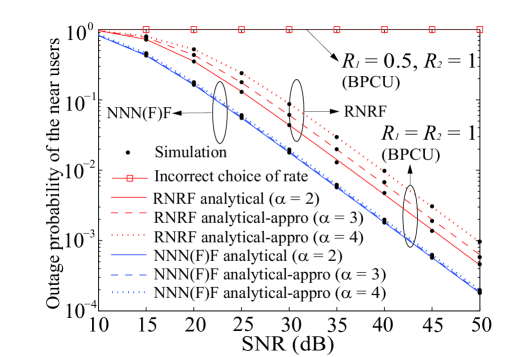
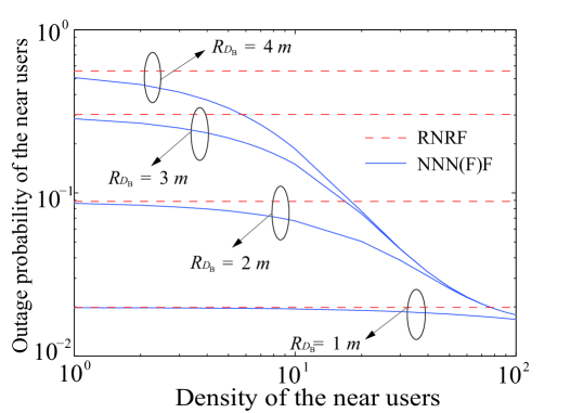
In this subsection, the outage probability achieved by the near users with different choices of density and path loss coefficients for the three user selection schemes is demonstrated. Note that the same user selection criterion is applied for the near users of NNNF and NNFF, we use NNN(F)F to represent these two selection schemes in Fig. 2, Fig. 3, and Fig. 4.

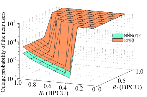
Fig. 2 plots the outage probability of the near users versus SNR with different path loss coefficients for both RNRF and NNN(F)F. The solid red and blue curves are for the special case α=2𝛼2\alpha=2 of RNRF and NNN(F)F, corresponding to the analytical results derived in (20) and (3), respectively. The dashed red and blue curves are for an arbitrary choice of α𝛼\alpha, corresponding to the analytical results derived in (14) and (29), respectively. Monte Carlo simulation results are marked as “\bullet” to verify our derivation. The figure shows precise agreement between the simulation and analytical curves. One can observe that by performing NNNF and NNFF (which we refer to as NNN(F)F in the figure), lower outage probability is achieved than with RNRF since shorter distances mean lower path loss and leads to better performance. The figure also demonstrates that as α𝛼\alpha increases, outage will occur more frequently because of higher path loss. For NNNF and NNFF, the performance is very close for different values of α𝛼\alpha. This is because we use the bounded path loss model (i.e. 1+diα>11superscriptsubscript𝑑i𝛼11+d_{\rm{i}}^{\alpha}>1) to ensure that the path loss is always larger than one. When selecting the nearest near user, disubscript𝑑id_{\rm{i}} will approach zero and the path loss will approach one, which makes the performance difference of the three selection schemes insignificant. It is worth noting that all curves have the same slopes, which indicates that the diversity gains of the schemes are the same. This phenomenon validates the insights we obtained from the analytical results derived in (26). Fig. 2 also shows that if the choices of rates for users are incorrect (i.e., R1=0.5subscript𝑅10.5R_{1}=0.5 and R2=1subscript𝑅21R_{2}=1 in this figure), the outage probability of the near users will be always one, which verifies the analytical results in (14) and (29).
Refer to caption
Figure 2: Outage probability of the near users versus SNR with different α𝛼\alpha, where RDB=2subscript𝑅subscript𝐷B2R_{{D_{\rm{B}}}}=2 m𝑚m, and λΦB=1subscript𝜆subscriptΦB1{\lambda_{{\Phi_{\rm{B}}}}}=1.

Fig. 3 plots the outage probability of the near users versus their density with different values of RDBsubscript𝑅subscript𝐷BR_{{D_{\rm{B}}}}. RNRF is also shown in the figure as a benchmark for comparison. Several observations are drawn as follows: 1) The outage probabilities of RNRF and NNN(F)F decrease with decreasing RDBsubscript𝑅subscript𝐷BR_{{D_{\rm{B}}}} because path loss is reduced; 2) The outage probability of NNN(F)F decreases as the density of the near users increases. This is due to the multiuser diversity gain, since there is an increasing number of the near users; 3) The outage probability of RNRF is a constant, i.e., independent of the density of near users, and is the outage ceiling of the NNN(F)F. This is due to the fact that no opportunistic user selection is carried out for RNRF; and 4) An outage floor exits even if the density of the near users goes to infinity. This is due to the bounded path loss model we have used. When the number of the near users exceeds a threshold, the selected near user will be very close to the source, which makes the path gain approach one.
Refer to caption
Figure 3: Outage probability of the near users versus density with different RDBsubscript𝑅subscript𝐷BR_{{D_{\rm{B}}}}, where λΦB=1subscript𝜆subscriptΦB1{\lambda_{{\Phi_{\rm{B}}}}}=1, and SNR=30𝑆𝑁𝑅30SNR=30 dB.

Fig. 4 plots the outage probability of the near users versus the rate of the near users and far users for both RNRF and NNN(F)F. One can observe that the outage of the near users occurs more frequently as the rate of the far user, R1subscript𝑅1R_{1}, increases. This is because in our proposed protocol, the near user BisubscriptBi\mathrm{B_{i}} needs to first decode xi1subscript𝑥𝑖1x_{i1} which is intended to the far user AisubscriptAi\mathrm{A_{i}}, and then decode its own message. Therefore increasing R1subscript𝑅1R_{1} makes it harder to decode xi1subscript𝑥𝑖1x_{i1}, which will lead to increased outages. An important observation is that incorrect choices of R1subscript𝑅1R_{1} and R2subscript𝑅2R_{2} will make the outage probability always one. Particularly, for the choice of R1subscript𝑅1R_{1}, it should satisfy the condition (|pi1|2|pi2|2τ1>0superscriptsubscript𝑝𝑖12superscriptsubscript𝑝𝑖22subscript𝜏10{\left|{{p_{i1}}}\right|^{2}}-{\left|{{p_{i2}}}\right|^{2}}{\tau_{1}}>0) in order to ensure that successive interference cancelation can be implemented. For the choice of R2subscript𝑅2R_{2}, it should satisfy the condition that the split energy for detecting xi1subscript𝑥𝑖1x_{i1} is also sufficient to detect xi2subscript𝑥𝑖2x_{i2} (εAiεBisubscript𝜀subscriptA𝑖subscript𝜀subscriptB𝑖{\varepsilon_{{{\rm{A}}_{i}}}}\geq{\varepsilon_{{{\rm{B}}_{i}}}}).

Refer to caption
Figure 4: Outage probability of the near users versus R1subscript𝑅1R_{1} and R2subscript𝑅2R_{2}, where α=2,RDB=2formulae-sequence𝛼2subscript𝑅subscript𝐷B2\alpha=2,R_{{D_{\rm{B}}}}=2 m𝑚m, and SNR=30𝑆𝑁𝑅30SNR=30 dB.

IV-B Outage Probability of the Far Users

In this subsection, we demonstrate the outage probability of the far users with different choices of the density, path loss coefficients, and user zone of the three user selection schemes.

Fig. 5 plots the outage probability of the far users versus SNR with different path loss coefficients of RNRF, NNNF, and NNFF. The dashed red, blue, and black curves circled together and pointed by α=2𝛼2\alpha=2, are the analytical approximations for the special case of RNRF, NNNF, and NNFF, which are obtained from (2), (4) and (5), respectively. The dashed red, blue, and black curves circled together and pointed by α=3𝛼3\alpha=3, are the analytical approximations for an arbitrary choice of α𝛼\alpha of RNRF, NNNF, and NNFF, which are obtained from (2), (4) and (5), respectively. We use the solid marked lines to represent the Monte Carlo simulation results for each case. As can be observed from the figure, the simulation and the analytical approximation are very close, particularly in the high SNR region. Several observations can be drawn as follows: 1) NNNF achieves the lowest outage probability among the three selection schemes since both the near and far users have the smallest path loss; 2) NNFF achieves lower outage than RNRF, which indicates that the distance of the near users has more impact than that of the far users; 3) it is clear that all of the curves in Fig. 5 have the same slopes, which indicates that the diversity gains of the far users for the three schemes are the same. In the diversity analysis, we showed that the diversity gain of the three selection schemes is two. The simulation validates the analytical results and indicates that the achievable diversity gain is the same for different user selection schemes.
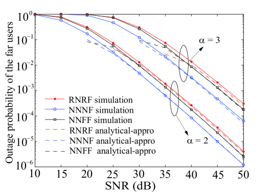
Refer to caption
Figure 5: Outage probability of the far users with different α𝛼\alpha, R1=0.3subscript𝑅10.3R_{1}=0.3 BPCU, RDA=10subscript𝑅subscript𝐷A10R_{{D_{\rm{A}}}}=10 m𝑚m, RDB=2subscript𝑅subscript𝐷B2R_{{D_{\rm{B}}}}=2 m𝑚m, RDC=8subscript𝑅subscript𝐷C8R_{{D_{\rm{C}}}}=8 m𝑚m, λΦA=1subscript𝜆subscriptΦA1{\lambda_{{\Phi_{\rm{A}}}}}=1, and λΦB=1subscript𝜆subscriptΦB1{\lambda_{{\Phi_{\rm{B}}}}}=1.

Fig. 6 plots the outage probability of the far users versus R1subscript𝑅1R_{1} with different RDCsubscript𝑅subscript𝐷CR_{{D_{\rm{C}}}} and RDBsubscript𝑅subscript𝐷BR_{{D_{\rm{B}}}}. One can observe that the outage probabilities of the three schemes increase as R1subscript𝑅1R_{1} increases. This is because increasing R1subscript𝑅1R_{1} will make the threshold of decoding higher, which in turn leads to more outage. It can also be observed that increasing the radius of the user zone for the far users will deteriorate the outage performance. The reason is that the path loss of the far users becomes larger.
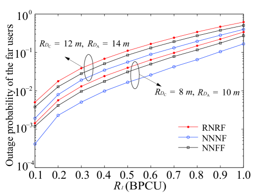
Refer to caption
Figure 6: Outage probability of the far users versus R1subscript𝑅1R_{1}, where α=2𝛼2\alpha=2, RDB=2subscript𝑅subscript𝐷B2R_{{D_{\rm{B}}}}=2 m𝑚m, and SNR=30𝑆𝑁𝑅30SNR=30 dB.

Fig. 7 plots the outage probability of the far users versus SNR for both cooperative NOMA and non-cooperative NOMA111It is common to use outage probability as a criterion to compare the performance of cooperative transmission and non-cooperative transmission schemes [14]. In the context of cooperative NOMA, the use of outage probability is particularly useful since the purpose of cooperative NOMA is to improve the reception reliability of the far users.. Several observations can be drawn as follows: 1) by using an energy constrained relay to perform cooperative NOMA transmission, the outage probability of the far users has a larger slope than that of non-cooperative NOMA, for all user selection schemes. This is due to the fact that cooperative NOMA can achieve a larger diversity gain and guarantees more reliable reception for the far users in the high SINR region; 2) NNNF achieves the lowest outage probability among these three selection schemes both for cooperative NOMA and non-cooperative NOMA because of its smallest path loss; 3) it is worth noting that NNFF has higher outage probability than RNRF in non-cooperative NOMA, however, it achieves lower outage probability than RNRF in cooperative NOMA. This phenomenon indicates that it is very helpful and necessary to apply cooperative NOMA in NNFF due to the largest performance gain over non-cooperative NOMA.
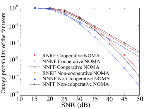
Refer to caption
Figure 7: Comparison of outage probability with non-cooperative NOMA, α=3𝛼3\alpha=3, R1=0.3subscript𝑅10.3R_{1}=0.3 BPCU, RDA=10subscript𝑅subscript𝐷A10R_{{D_{\rm{A}}}}=10 m𝑚m, RDB=2subscript𝑅subscript𝐷B2R_{{D_{\rm{B}}}}=2 m𝑚m, RDC=8subscript𝑅subscript𝐷C8R_{{D_{\rm{C}}}}=8 m𝑚m, λΦA=1subscript𝜆subscriptΦA1{\lambda_{{\Phi_{\rm{A}}}}}=1, and λΦB=1subscript𝜆subscriptΦB1{\lambda_{{\Phi_{\rm{B}}}}}=1.

IV-C Throughput in Delay-Sensitive Transmission Mode

Fig. 8 plots the system throughput versus SNR with different targeted rates. One can observe that NNNF achieves the highest throughput since it has the lowest outage probability among three selection schemes. The figure also demonstrates the existence of the throughput ceilings in the high SNR region. This is due to the fact that the outage probability is approaching zero and the throughput is determined only by the targeted data rate. It is worth noting that increasing R2subscript𝑅2R_{2} from R2=0.5subscript𝑅20.5R_{2}=0.5 BPCU to R2=1subscript𝑅21R_{2}=1 BPCU can improve the throughput; however, for the case R2=2subscript𝑅22R_{2}=2 BPCU, the throughput is lowered. This is because, in the latter case, the energy remaining for information decoding is not sufficient for message detection of the near user, and hence an outage occurs, which in turn affects the throughput. Therefore, we see that it is important to select appropriate transmission rates when designing practical NOMA downlink transmission systems.
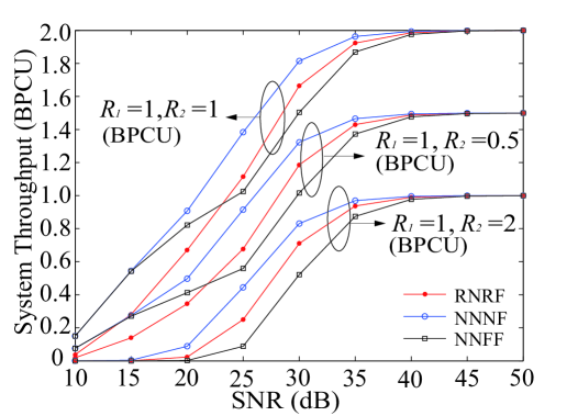
Refer to caption
Figure 8: System throughput in delay-sensitive mode versus SNR with different rate, α=2𝛼2\alpha=2, RDA=10subscript𝑅subscript𝐷A10R_{{D_{\rm{A}}}}=10 m𝑚m, RDB=2subscript𝑅subscript𝐷B2R_{{D_{\rm{B}}}}=2 m𝑚m, RDC=8subscript𝑅subscript𝐷C8R_{{D_{\rm{C}}}}=8 m𝑚m, λΦA=1subscript𝜆subscriptΦA1{\lambda_{{\Phi_{\rm{A}}}}}=1, and λΦB=1subscript𝜆subscriptΦB1{\lambda_{{\Phi_{\rm{B}}}}}=1.

V Conclusions

In this paper, the application of SWIPT to NOMA has been considered. A novel cooperative SWIPT NOMA protocol with three different user selection criteria has been proposed. We have used the stochastic geometric approach to provide a complete framework to model the locations of users and evaluate the performance of the proposed user selection schemes. Closed-form results have been derived in terms of outage probability and delay-sensitive throughput to determine the system performance. The diversity gain of the three user selection schemes has also been characterized and proved to be the same as that of a conventional cooperative network. For the proposed protocol, the decreasing rate of the outage probability of far users is lnSNRSNR2𝑆𝑁𝑅𝑆𝑁superscript𝑅2\frac{{\ln SNR}}{{SN{R^{2}}}} while it is 1SNR21𝑆𝑁superscript𝑅2\frac{1}{{SN{R^{2}}}} for a conventional cooperative network. Numerical results have been presented to validate our analysis. We conclude that by carefully choosing the parameters of the network, (e.g., transmission rate or power splitting coefficient), acceptable system performance can be guaranteed even if the users do not use their own batteries to power the relay transmission.

Appendix A: Proof of Theorem 2

Substituting (4) and (12) into (III-A2), the outage probability can be expressed as follows:

PAi=subscript𝑃subscriptAiabsent\displaystyle{P_{{{\rm{A_{i}}}}}}= Pr(γAi,MRCxi1<τ1,ρ|hBi|2|pi1|2ρ|hBi|2|pi2|2+1+dBiα>τ1)Θ1subscriptPrsuperscriptsubscript𝛾subscriptAiMRCsubscript𝑥𝑖1subscript𝜏1𝜌superscriptsubscriptsubscriptBi2superscriptsubscript𝑝𝑖12𝜌superscriptsubscriptsubscriptBi2superscriptsubscript𝑝𝑖221superscriptsubscript𝑑subscriptBi𝛼subscript𝜏1subscriptΘ1\displaystyle\underbrace{\Pr\left({\gamma_{{{\rm{A}}_{\rm{i}}},{\rm{MRC}}}^{{x_{i1}}}<{\tau_{1}},\frac{{\rho{{\left|{{h_{{{\rm{B}}_{\rm{i}}}}}}\right|}^{2}}{{\left|{{p_{i1}}}\right|}^{2}}}}{{\rho{{\left|{{h_{{{\rm{B}}_{\rm{i}}}}}}\right|}^{2}}{{\left|{{p_{i2}}}\right|}^{2}}+1+d_{{{\rm{B}}_{\rm{i}}}}^{\alpha}}}>{\tau_{1}}}\right)}_{{\Theta_{1}}}
+Pr(γS,Aixi1<τ1,ρ|hBi|2|pi1|2ρ|hBi|2|pi2|2+1+dBiα<τ1)Θ2,subscriptPrsuperscriptsubscript𝛾SsubscriptAisubscript𝑥𝑖1subscript𝜏1𝜌superscriptsubscriptsubscriptBi2superscriptsubscript𝑝𝑖12𝜌superscriptsubscriptsubscriptBi2superscriptsubscript𝑝𝑖221superscriptsubscript𝑑subscriptBi𝛼subscript𝜏1subscriptΘ2\displaystyle+\underbrace{\Pr\left({\gamma_{{\rm{S}},{{\rm{A}}_{\rm{i}}}}^{{x_{i1}}}<{\tau_{1}},\frac{{\rho{{\left|{{h_{{{\rm{B}}_{\rm{i}}}}}}\right|}^{2}}{{\left|{{p_{i1}}}\right|}^{2}}}}{{\rho{{\left|{{h_{{{\rm{B}}_{\rm{i}}}}}}\right|}^{2}}{{\left|{{p_{i2}}}\right|}^{2}}+1+d_{{{\rm{B}}_{\rm{i}}}}^{\alpha}}}<{\tau_{1}}}\right)}_{{\Theta_{2}}}, (A.1)

We express Θ1subscriptΘ1{\Theta_{1}} as (Appendix A: Proof of Theorem 2) on the top of next page

Θ1=Pr(Zi<τ1ρXi|pi1|2ρXi|pi2|2+1ηρ(YiεAi),Xi<εAi,Yi>εAi)subscriptΘ1Prsubscript𝑍𝑖subscript𝜏1𝜌subscript𝑋𝑖superscriptsubscript𝑝𝑖12𝜌subscript𝑋𝑖superscriptsubscript𝑝𝑖221𝜂𝜌subscript𝑌𝑖subscript𝜀subscriptA𝑖subscript𝑋𝑖subscript𝜀subscriptA𝑖subscript𝑌𝑖subscript𝜀subscriptA𝑖\displaystyle{\Theta_{1}}=\Pr\left({{Z_{i}}<\frac{{{\tau_{1}}-\frac{{\rho{X_{i}}{{\left|{{p_{i1}}}\right|}^{2}}}}{{\rho{X_{i}}{{\left|{{p_{i2}}}\right|}^{2}}+1}}}}{{\eta\rho\left({{Y_{i}}-{\varepsilon_{{{\rm{A}}_{i}}}}}\right)}},{X_{i}}<{\varepsilon_{{{\rm{A}}_{i}}}},{Y_{i}}>{\varepsilon_{{{\rm{A}}_{i}}}}}\right)
=\displaystyle= DBDA0εAiεAi(1e(1+dCiα)τ1ρx|pi1|2ρx|pi2|2+1ηρ(yεAi))fYi(y)𝑑yΞfXi(x)𝑑xfWAi(ωAi)𝑑ωAifWBi(ωBi)𝑑ωBi,subscriptsubscript𝐷Bsubscriptsubscript𝐷Asuperscriptsubscript0subscript𝜀subscriptA𝑖subscriptsuperscriptsubscriptsubscript𝜀subscriptA𝑖1superscript𝑒1superscriptsubscript𝑑subscriptCi𝛼subscript𝜏1𝜌𝑥superscriptsubscript𝑝𝑖12𝜌𝑥superscriptsubscript𝑝𝑖221𝜂𝜌𝑦subscript𝜀subscriptA𝑖subscript𝑓subscript𝑌𝑖𝑦differential-d𝑦Ξsubscript𝑓subscript𝑋𝑖𝑥differential-d𝑥subscript𝑓subscript𝑊subscriptAisubscript𝜔subscriptAidifferential-dsubscript𝜔subscriptAisubscript𝑓subscript𝑊subscriptBisubscript𝜔subscriptBidifferential-dsubscript𝜔subscriptBi\displaystyle\int\limits_{{{D_{{{\rm{B}}}}}}}{\int\limits_{{D_{{{\rm{A}}}}}}{\int_{0}^{{\varepsilon_{{{\rm{A}}_{i}}}}}{\underbrace{\int_{{\varepsilon_{{{\rm{A}}_{i}}}}}^{\infty}{\left({1-{e^{-\left({1+d_{{{\rm{C}}_{\rm{i}}}}^{\alpha}}\right)\frac{{{\tau_{1}}-\frac{{\rho x{{\left|{{p_{i1}}}\right|}^{2}}}}{{\rho x{{\left|{{p_{i2}}}\right|}^{2}}+1}}}}{{\eta\rho\left({y-{\varepsilon_{{{\rm{A}}_{i}}}}}\right)}}}}}\right){f_{Y_{i}}}\left(y\right)dy}}_{\Xi}}}}{f_{X_{i}}}\left(x\right)dx{f_{{W_{{{\rm{A}}_{\rm{i}}}}}}}\left({{\omega_{{{\rm{A_{i}}}}}}}\right)d{\omega_{{{\rm{A_{i}}}}}}{f_{{W_{{{\rm{B}}_{\rm{i}}}}}}}\left({{\omega_{{{\rm{B_{i}}}}}}}\right)d{\omega_{{{\rm{B_{i}}}}}}, (A.2)

where fXi(x)=(1+dAiα)e(1+dAiα)xsubscript𝑓subscript𝑋𝑖𝑥1superscriptsubscript𝑑subscriptAi𝛼superscript𝑒1superscriptsubscript𝑑subscriptAi𝛼𝑥{f_{X_{i}}}\left(x\right)=\left({1+d_{{{\rm{A}}_{\rm{i}}}}^{\alpha}}\right){e^{-\left({1+d_{{{\rm{A}}_{\rm{i}}}}^{\alpha}}\right)x}}, and fYi(y)=(1+dBiα)e(1+dBiα)ysubscript𝑓subscript𝑌𝑖𝑦1superscriptsubscript𝑑subscriptBi𝛼superscript𝑒1superscriptsubscript𝑑subscriptBi𝛼𝑦{f_{Y_{i}}}\left(y\right)=\left({1+d_{{{\rm{B}}_{\rm{i}}}}^{\alpha}}\right){e^{-\left({1+d_{{{\rm{B}}_{\rm{i}}}}^{\alpha}}\right)y}}.

Based on (Appendix A: Proof of Theorem 2), using t=yεAi𝑡𝑦subscript𝜀subscriptA𝑖t=y-{\varepsilon_{{{\rm{A}}_{i}}}}, we calculate ΞΞ{\Xi} as follows:

Ξ=Ξabsent\displaystyle{\Xi}= 0(1e(1+dCiα)τρx|pi1|2ρx|pi2|2+1ηρt)superscriptsubscript01superscript𝑒1superscriptsubscript𝑑subscriptCi𝛼𝜏𝜌𝑥superscriptsubscript𝑝𝑖12𝜌𝑥superscriptsubscript𝑝𝑖221𝜂𝜌𝑡\displaystyle\int_{0}^{\infty}{\left({1-{e^{-\left({1+d_{{{\rm{C}}_{\rm{i}}}}^{\alpha}}\right)\frac{{\tau-\frac{{\rho x{{\left|{{p_{i1}}}\right|}^{2}}}}{{\rho x{{\left|{{p_{i2}}}\right|}^{2}}+1}}}}{{\eta\rho t}}}}}\right)}
×(1+dBiα)e(1+dBiα)(t+εAi)dt.absent1superscriptsubscript𝑑subscriptBi𝛼superscript𝑒1superscriptsubscript𝑑subscriptBi𝛼𝑡subscript𝜀subscriptA𝑖𝑑𝑡\displaystyle\times\left({1+d_{{{\rm{B}}_{\rm{i}}}}^{\alpha}}\right){e^{-\left({1+d_{{{\rm{B}}_{\rm{i}}}}^{\alpha}}\right)\left({t+{\varepsilon_{{{\rm{A}}_{i}}}}}\right)}}dt. (A.3)

Applying [15, Eq. (3.324)], we rewrite (Appendix A: Proof of Theorem 2) as follows:

Ξ=e(1+dBiα)εAi(12χΛK1(2χΛ)),Ξsuperscript𝑒1superscriptsubscript𝑑subscriptBi𝛼subscript𝜀subscriptA𝑖12𝜒Λsubscript𝐾12𝜒Λ\displaystyle\Xi={e^{-\left({1+d_{{{\rm{B}}_{\rm{i}}}}^{\alpha}}\right){\varepsilon_{{{\rm{A}}_{i}}}}}}\left({1-2\sqrt{\chi\Lambda}{K_{1}}\left({2\sqrt{\chi\Lambda}}\right)}\right), (A.4)

where Λ=(1+dBiα)(1+dCiα)ηρΛ1superscriptsubscript𝑑subscriptBi𝛼1superscriptsubscript𝑑subscriptCi𝛼𝜂𝜌\Lambda=\frac{{\left({1+d_{{{\rm{B}}_{\rm{i}}}}^{\alpha}}\right)\left({1+d_{{{\rm{C}}_{\rm{i}}}}^{\alpha}}\right)}}{{\eta\rho}} and χ=τ1ρx|pi1|2ρx|pi2|2+1𝜒subscript𝜏1𝜌𝑥superscriptsubscript𝑝𝑖12𝜌𝑥superscriptsubscript𝑝𝑖221\chi={\tau_{1}}-\frac{{\rho x{{\left|{{p_{i1}}}\right|}^{2}}}}{{\rho x{{\left|{{p_{i2}}}\right|}^{2}}+1}}.

We use the series representation of Bessel functions to obtain the high SNR approximation which is expressed as follows:

xK1(x)1+x22(lnx2+c0),𝑥subscript𝐾1𝑥1superscript𝑥22𝑥2subscript𝑐0\displaystyle x{K_{1}}\left(x\right)\approx 1+\frac{{{x^{2}}}}{2}\left({\ln\frac{x}{2}+{c_{0}}}\right), (A.5)

where K1()subscript𝐾1{K_{1}}\left(\cdot\right) is the modified Bessel function for the seconde kind, c0=φ(1)2φ(2)2subscript𝑐0𝜑12𝜑22{c_{0}}=-\frac{{\varphi\left(1\right)}}{2}-\frac{{\varphi\left(2\right)}}{2}, and φ()𝜑\varphi\left(\cdot\right) denotes the psi function [15].

To obtain the high SNR approximation of (A.4) and using (A.5), we obtain

ΞχΛ(lnχΛ+2c0).Ξ𝜒Λ𝜒Λ2subscript𝑐0\displaystyle\Xi\approx-\chi\Lambda\left({\ln\chi\Lambda+2{c_{0}}}\right). (A.6)

Substituting (A.6) into (Appendix A: Proof of Theorem 2), we rewrite (Appendix A: Proof of Theorem 2) as follows:

Θ1=subscriptΘ1absent\displaystyle{\Theta_{1}}= 0εAiχDAiΛe(1+dAiα)xsuperscriptsubscript0subscript𝜀subscriptA𝑖𝜒subscriptsubscript𝐷subscriptAiΛsuperscript𝑒1superscriptsubscript𝑑subscriptAi𝛼𝑥\displaystyle-\int_{0}^{{\varepsilon_{{{\rm{A}}_{i}}}}}\chi\int\limits_{{D_{{{\rm{A}}_{\rm{i}}}}}}{\Lambda{e^{-\left({1+d_{{{\rm{A}}_{\rm{i}}}}^{\alpha}}\right)x}}}
×DBi(1+dBiα)(lnχΛ+2c0)fWBi(ωBi)𝑑ωBiΦabsentsubscriptsubscriptsubscript𝐷subscriptBi1superscriptsubscript𝑑subscriptBi𝛼𝜒Λ2subscript𝑐0subscript𝑓subscript𝑊subscriptBisubscript𝜔subscriptBidifferential-dsubscript𝜔subscriptBiΦ\displaystyle\times\underbrace{\int\limits_{{D_{{{\rm{B}}_{\rm{i}}}}}}{\left({1+d_{{{\rm{B}}_{\rm{i}}}}^{\alpha}}\right)\left({\ln\chi\Lambda+2{c_{0}}}\right){f_{{W_{{{\rm{B}}_{\rm{i}}}}}}}\left({{\omega_{{{\rm{B}}_{\rm{i}}}}}}\right)d{\omega_{{{\rm{B}}_{\rm{i}}}}}}}_{\Phi}
fWAi(ωAi)dωAidx.subscript𝑓subscript𝑊subscriptAisubscript𝜔subscriptAi𝑑subscript𝜔subscriptAi𝑑𝑥\displaystyle{f_{{W_{{{\rm{A}}_{\rm{i}}}}}}}\left({{\omega_{{{\rm{A}}_{\rm{i}}}}}}\right)d{\omega_{{{\rm{A}}_{\rm{i}}}}}dx. (A.7)

Since dCi=dAi2+dBi22dAidBicos(θi)subscript𝑑subscriptCisuperscriptsubscript𝑑subscriptAi2superscriptsubscript𝑑subscriptBi22subscript𝑑subscriptAisubscript𝑑subscriptBisubscript𝜃𝑖{d_{{{\rm{C}}_{\rm{i}}}}}=\sqrt{d_{{{\rm{A}}_{\rm{i}}}}^{2}+d_{{{\rm{B}}_{\rm{i}}}}^{2}-2{d_{{{\rm{A}}_{\rm{i}}}}}{d_{{{\rm{B}}_{\rm{i}}}}}\cos\left({{\theta_{i}}}\right)} and RDCRDBmuch-greater-thansubscript𝑅subscript𝐷Csubscript𝑅subscript𝐷B{R_{{D_{\rm{C}}}}}\gg{R_{{D_{\rm{B}}}}}, we can approximate the distance as dAidCisubscript𝑑subscriptAisubscript𝑑subscriptCi{d_{{{\rm{A}}_{\rm{i}}}}}\approx{d_{{{\rm{C}}_{\rm{i}}}}}. Applying (16), we calculate ΦΦ\Phi as follows:

ΦΦabsent\displaystyle\Phi\approx 2RDB20RDB(1+rα)(lnm0(1+rα)+2c0)r𝑑r,2superscriptsubscript𝑅subscript𝐷B2superscriptsubscript0subscript𝑅subscript𝐷B1superscript𝑟𝛼subscript𝑚01superscript𝑟𝛼2subscript𝑐0𝑟differential-d𝑟\displaystyle\frac{2}{{R_{{D_{{{\rm{B}}}}}}^{2}}}\int_{0}^{{R_{{D_{\rm{B}}}}}}{\left({1+{r^{\alpha}}}\right)\left({\ln{m_{0}}\left({1+{r^{\alpha}}}\right)+2{c_{0}}}\right)rdr}, (A.8)

where m0=χ(1+dCiα)ηρχ(1+dAiα)ηρsubscript𝑚0𝜒1superscriptsubscript𝑑subscriptCi𝛼𝜂𝜌𝜒1superscriptsubscript𝑑subscriptAi𝛼𝜂𝜌{m_{0}}=\frac{{\chi\left({1+d_{{{\rm{C}}_{\rm{i}}}}^{\alpha}}\right)}}{{\eta\rho}}\approx\frac{{\chi\left({1+d_{{{\rm{A}}_{\rm{i}}}}^{\alpha}}\right)}}{{\eta\rho}}.

For an arbitrary choice of α𝛼\alpha, the integral in (A.8) is mathematically intractable, we use Gaussian-Chebyshev quadrature to find the approximation. Then ΦΦ\Phi can be approximated as follows:

ΦωN2n=1N(1ϕn2cn(lnm0cn+2c0)(ϕn+1)).Φsubscript𝜔𝑁2superscriptsubscript𝑛1𝑁1superscriptsubscriptitalic-ϕ𝑛2subscript𝑐𝑛subscript𝑚0subscript𝑐𝑛2subscript𝑐0subscriptitalic-ϕ𝑛1\displaystyle\Phi\approx\frac{{{\omega_{N}}}}{2}\sum\limits_{n=1}^{N}{\left({\sqrt{1-{\phi_{n}}^{2}}{c_{n}}\left({\ln{m_{0}}{c_{n}}+2{c_{0}}}\right)\left({{\phi_{n}}+1}\right)}\right)}. (A.9)

Substituting (A.9) into (Appendix A: Proof of Theorem 2), we rewrite (Appendix A: Proof of Theorem 2) as follows:

Θ1=ωNRDA2RDC20εAiχηρn=1N(ϕn+1)1ϕn2subscriptΘ1subscript𝜔𝑁superscriptsubscript𝑅subscript𝐷A2superscriptsubscript𝑅subscript𝐷C2superscriptsubscript0subscript𝜀subscriptA𝑖𝜒𝜂𝜌superscriptsubscript𝑛1𝑁subscriptitalic-ϕ𝑛11superscriptsubscriptitalic-ϕ𝑛2\displaystyle\Theta_{1}=-\frac{{{\omega_{N}}}}{{R_{{D_{\rm{A}}}}^{2}-R_{{D_{\rm{C}}}}^{2}}}\int_{0}^{{\varepsilon_{{{\rm{A}}_{i}}}}}{\frac{\chi}{{\eta\rho}}}\sum\limits_{n=1}^{N}{\left({{\phi_{n}}+1}\right)\sqrt{1-{\phi_{n}}^{2}}}
RDCRDAr(1+rα)2e(1+rα)xcn(lnχ(1+rα)ηρcn+2c0)𝑑rΔsubscriptsuperscriptsubscriptsubscript𝑅subscript𝐷Csubscript𝑅subscript𝐷A𝑟superscript1superscript𝑟𝛼2superscript𝑒1superscript𝑟𝛼𝑥subscript𝑐𝑛𝜒1superscript𝑟𝛼𝜂𝜌subscript𝑐𝑛2subscript𝑐0differential-d𝑟Δ\displaystyle\underbrace{\int_{{R_{{D_{\rm{C}}}}}}^{{R_{{D_{\rm{A}}}}}}{r{{\left({1+{r^{\alpha}}}\right)}^{2}}{e^{-\left({1+{r^{\alpha}}}\right)x}}{c_{n}}\left({\ln\frac{{\chi\left({1+{r^{\alpha}}}\right)}}{{\eta\rho}}{c_{n}}+2{c_{0}}}\right)}dr}_{\Delta}
dx.𝑑𝑥\displaystyle dx. (A.10)

Similarly as above, we use Gaussian-Chebyshev quadrature to find an approximation of ΔΔ\Delta in (Appendix A: Proof of Theorem 2) as follows:

ΔΔabsent\displaystyle\Delta\approx ωK(RDARDC)2k=1K1ψk2sk(1+skα)2subscript𝜔𝐾subscript𝑅subscript𝐷Asubscript𝑅subscript𝐷C2superscriptsubscript𝑘1𝐾1superscriptsubscript𝜓𝑘2subscript𝑠𝑘superscript1superscriptsubscript𝑠𝑘𝛼2\displaystyle\frac{{{\omega_{K}}\left({{R_{{D_{\rm{A}}}}}-{R_{{D_{\rm{C}}}}}}\right)}}{2}\sum\limits_{k=1}^{K}{\sqrt{1-\psi_{k}^{2}}{s_{k}}{{\left({1+s_{k}^{\alpha}}\right)}^{2}}}
×e(1+skα)xcn(lnχ(1+skα)ηρcn+2c0).absentsuperscript𝑒1superscriptsubscript𝑠𝑘𝛼𝑥subscript𝑐𝑛𝜒1superscriptsubscript𝑠𝑘𝛼𝜂𝜌subscript𝑐𝑛2subscript𝑐0\displaystyle\times{e^{-\left({1+s_{k}^{\alpha}}\right)x}}{c_{n}}\left({\ln\frac{{\chi\left({1+s_{k}^{\alpha}}\right)}}{{\eta\rho}}{c_{n}}+2{c_{0}}}\right). (A.11)

Substituting (Appendix A: Proof of Theorem 2) into (Appendix A: Proof of Theorem 2), we rewrite (Appendix A: Proof of Theorem 2) as follows:

Θ1=subscriptΘ1absent\displaystyle\Theta_{1}= a2n=1N(ϕn+1)1ϕn2cnk=1K1ψk2sk(1+skα)2subscript𝑎2superscriptsubscript𝑛1𝑁subscriptitalic-ϕ𝑛11superscriptsubscriptitalic-ϕ𝑛2subscript𝑐𝑛superscriptsubscript𝑘1𝐾1superscriptsubscript𝜓𝑘2subscript𝑠𝑘superscript1superscriptsubscript𝑠𝑘𝛼2\displaystyle{a_{2}}\sum\limits_{n=1}^{N}{\left({{\phi_{n}}+1}\right)\sqrt{1-{\phi_{n}}^{2}}{c_{n}}\sum\limits_{k=1}^{K}{\sqrt{1-\psi_{k}^{2}}{s_{k}}{{\left({1+s_{k}^{\alpha}}\right)}^{2}}}}
×0εAiχe(1+skα)x(lnχ(1+skα)ηρcn+2c0)𝑑xΨ,absentsubscriptsuperscriptsubscript0subscript𝜀subscriptA𝑖𝜒superscript𝑒1superscriptsubscript𝑠𝑘𝛼𝑥𝜒1superscriptsubscript𝑠𝑘𝛼𝜂𝜌subscript𝑐𝑛2subscript𝑐0differential-d𝑥Ψ\displaystyle\times\underbrace{\int_{0}^{{\varepsilon_{{{\rm{A}}_{i}}}}}{\chi{e^{-\left({1+s_{k}^{\alpha}}\right)x}}\left({\ln\frac{{\chi\left({1+s_{k}^{\alpha}}\right)}}{{\eta\rho}}{c_{n}}+2{c_{0}}}\right)dx}}_{\Psi}, (A.12)

where a2=ωNωK2(RDA+RDC)ηρsubscript𝑎2subscript𝜔𝑁subscript𝜔𝐾2subscript𝑅subscript𝐷Asubscript𝑅subscript𝐷C𝜂𝜌{a_{2}}=-\frac{{{\omega_{N}}{\omega_{K}}}}{{2\left({{R_{{D_{\rm{A}}}}}+{R_{{D_{\rm{C}}}}}}\right)\eta\rho}}.

Similarly, we use Gaussian-Chebyshev quadrature to find an approximation of ΨΨ\Psi in (Appendix A: Proof of Theorem 2) as follows:

ΨΨabsent\displaystyle\Psi\approx ωMεAi2m=1M1φm2e(1+skα)tmsubscript𝜔𝑀subscript𝜀subscriptA𝑖2superscriptsubscript𝑚1𝑀1superscriptsubscript𝜑𝑚2superscript𝑒1superscriptsubscript𝑠𝑘𝛼subscript𝑡𝑚\displaystyle\frac{{{\omega_{M}}{\varepsilon_{{{\rm{A}}_{i}}}}}}{2}\sum\limits_{m=1}^{M}{\sqrt{1-\varphi_{m}^{2}}{e^{-\left({1+s_{k}^{\alpha}}\right){t_{m}}}}}
×χtm(lnχtm(1+skα)ηρcn+2c0).absentsubscript𝜒subscript𝑡𝑚subscript𝜒subscript𝑡𝑚1superscriptsubscript𝑠𝑘𝛼𝜂𝜌subscript𝑐𝑛2subscript𝑐0\displaystyle\times{\chi_{{t_{m}}}}\left({\ln\frac{{{\chi_{{t_{m}}}}\left({1+s_{k}^{\alpha}}\right)}}{{\eta\rho}}{c_{n}}+2{c_{0}}}\right). (A.13)

Substituting (Appendix A: Proof of Theorem 2) into (Appendix A: Proof of Theorem 2), we obtain

Θ1ζ1n=1N(ϕn+1)1ϕn2cnk=1K1ψk2sk(1+skα)2subscriptΘ1subscript𝜁1superscriptsubscript𝑛1𝑁subscriptitalic-ϕ𝑛11superscriptsubscriptitalic-ϕ𝑛2subscript𝑐𝑛superscriptsubscript𝑘1𝐾1superscriptsubscript𝜓𝑘2subscript𝑠𝑘superscript1superscriptsubscript𝑠𝑘𝛼2\displaystyle\Theta_{1}\approx\zeta_{1}\sum\limits_{n=1}^{N}{\left({{\phi_{n}}+1}\right)\sqrt{1-{\phi_{n}}^{2}}}{c_{n}}\sum\limits_{k=1}^{K}{\sqrt{1-\psi_{k}^{2}}{s_{k}}{{\left({1+s_{k}^{\alpha}}\right)}^{2}}}
m=1M1φm2e(1+skα)tmχtm(lnχtm(1+skα)ηρcn+2c0).superscriptsubscript𝑚1𝑀1superscriptsubscript𝜑𝑚2superscript𝑒1superscriptsubscript𝑠𝑘𝛼subscript𝑡𝑚subscript𝜒subscript𝑡𝑚subscript𝜒subscript𝑡𝑚1superscriptsubscript𝑠𝑘𝛼𝜂𝜌subscript𝑐𝑛2subscript𝑐0\displaystyle\sum\limits_{m=1}^{M}{\sqrt{1-\varphi_{m}^{2}}{e^{-\left({1+s_{k}^{\alpha}}\right){t_{m}}}}{\chi_{{t_{m}}}}\left({\ln\frac{{{\chi_{{t_{m}}}}\left({1+s_{k}^{\alpha}}\right)}}{{\eta\rho}}{c_{n}}+2{c_{0}}}\right)}. (A.14)

We express Θ2subscriptΘ2{\Theta_{2}} as follows:

Θ2=subscriptΘ2absent\displaystyle{\Theta_{2}}= Pr(Xi<εAi)Pr(Yi<εAi).Prsubscript𝑋𝑖subscript𝜀subscriptA𝑖Prsubscript𝑌𝑖subscript𝜀subscriptA𝑖\displaystyle\Pr\left({{X_{i}}<{\varepsilon_{{{\rm{A}}_{i}}}}}\right)\Pr\left({{Y_{i}}<{\varepsilon_{{{\rm{A}}_{i}}}}}\right). (A.15)

The CDF of Xisubscript𝑋𝑖X_{i} for AisubscriptAi{\rm{A_{i}}} is given by

FXi(ε)subscript𝐹subscript𝑋𝑖𝜀\displaystyle{F_{X_{i}}}\left(\varepsilon\right) =D(1e(1+dAiα)ε)fWAi(ωAi)𝑑ωAiabsentsubscript𝐷1superscript𝑒1superscriptsubscript𝑑subscriptAi𝛼𝜀subscript𝑓subscript𝑊subscriptAisubscript𝜔subscriptAidifferential-dsubscript𝜔subscriptAi\displaystyle=\int\limits_{D}{\left({1-{e^{-\left({1+d_{{{\rm{A}}_{\rm{i}}}}^{\alpha}}\right)\varepsilon}}}\right){f_{{W_{{{\rm{A}}_{\rm{i}}}}}}}\left({{\omega_{{{\rm{A}}_{\rm{i}}}}}}\right)d{\omega_{{{\rm{A}}_{\rm{i}}}}}}
=2RDA2RDC2RDCRDA(1e(1+rα)ε)r𝑑r.absent2superscriptsubscript𝑅subscript𝐷A2superscriptsubscript𝑅subscript𝐷C2superscriptsubscriptsubscript𝑅subscript𝐷Csubscript𝑅subscript𝐷A1superscript𝑒1superscript𝑟𝛼𝜀𝑟differential-d𝑟\displaystyle=\frac{2}{{R_{{D_{\rm{A}}}}^{2}-R_{{D_{\rm{C}}}}^{2}}}\int_{{R_{{D_{\rm{C}}}}}}^{{R_{{D_{\rm{A}}}}}}{\left({1-{e^{-\left({1+{r^{\alpha}}}\right)\varepsilon}}}\right)rdr}. (A.16)

For an arbitrary choice of α𝛼\alpha, similarly to (19), we provide Gaussian-Chebyshev quadrature to find the approximation for the CDF of Xisubscript𝑋𝑖X_{i}. We rewrite (Appendix A: Proof of Theorem 2) as follows:

FXi(ε)ωKRDA+RDCk=1K1ψk2(1e(1+skα)ε)sk.subscript𝐹subscript𝑋𝑖𝜀subscript𝜔𝐾subscript𝑅subscript𝐷Asubscript𝑅subscript𝐷Csuperscriptsubscript𝑘1𝐾1superscriptsubscript𝜓𝑘21superscript𝑒1superscriptsubscript𝑠𝑘𝛼𝜀subscript𝑠𝑘\displaystyle{F_{X_{i}}}\left(\varepsilon\right)\approx\frac{{{\omega_{K}}}}{{{R_{{D_{\rm{A}}}}}+{R_{{D_{\rm{C}}}}}}}\sum\limits_{k=1}^{K}{\sqrt{1-{\psi_{k}}^{2}}\left({1-{e^{-(1+s_{k}^{\alpha})\varepsilon}}}\right){s_{k}}}. (A.17)

When ε0𝜀0\varepsilon\to 0, a high SNR approximation of the (A.17) is given by

FXi(ε)ωKεRDA+RDCk=1K1ψk2(1+skα)sk.subscript𝐹subscript𝑋𝑖𝜀subscript𝜔𝐾𝜀subscript𝑅subscript𝐷Asubscript𝑅subscript𝐷Csuperscriptsubscript𝑘1𝐾1superscriptsubscript𝜓𝑘21superscriptsubscript𝑠𝑘𝛼subscript𝑠𝑘\displaystyle{F_{X_{i}}}\left(\varepsilon\right)\approx\frac{{{\omega_{K}}\varepsilon}}{{{R_{{D_{\rm{A}}}}}+{R_{{D_{\rm{C}}}}}}}\sum\limits_{k=1}^{K}{\sqrt{1-{\psi_{k}}^{2}}(1+s_{k}^{\alpha}){s_{k}}}. (A.18)

Substituting (A.18) and (19) into (A.15), we can obtain the approximation for the general case as follows:

Θ2a1n=1N1ϕn2cn(ϕn+1)k=1K1ψk2(1+skα)sk.subscriptΘ2subscript𝑎1superscriptsubscript𝑛1𝑁1superscriptsubscriptitalic-ϕ𝑛2subscript𝑐𝑛subscriptitalic-ϕ𝑛1superscriptsubscript𝑘1𝐾1superscriptsubscript𝜓𝑘21superscriptsubscript𝑠𝑘𝛼subscript𝑠𝑘\displaystyle{\Theta_{2}}\approx{a_{1}}\sum\limits_{n=1}^{N}{\sqrt{1-{\phi_{n}}^{2}}{c_{n}}\left({{\phi_{n}}+1}\right)}\sum\limits_{k=1}^{K}{\sqrt{1-{\psi_{k}}^{2}}(1+s_{k}^{\alpha}){s_{k}}}. (A.19)

Combining (Appendix A: Proof of Theorem 2) and (A.19), we can obtain (2).

The proof is completed.

Appendix B: Proof of Corollary 2

For the special case α=2𝛼2\alpha=2, and let λ=(1+r2)𝜆1superscript𝑟2\lambda=\left({1+{r^{2}}}\right), we rewrite (A.8) as follows:

Φ|α=2=evaluated-atΦ𝛼2absent\displaystyle{\left.\Phi\right|_{\alpha=2}}= 1RDB211+RDB2λ(lnm0λ+2c0)𝑑λ1superscriptsubscript𝑅subscript𝐷B2superscriptsubscript11superscriptsubscript𝑅subscript𝐷B2𝜆subscript𝑚superscript0𝜆2subscript𝑐0differential-d𝜆\displaystyle\frac{1}{{R_{{D_{\rm{B}}}}^{2}}}\int_{1}^{1+R_{{D_{\rm{B}}}}^{2}}{\lambda\left({\ln{m_{{0^{*}}}}\lambda+2{c_{0}}}\right)d\lambda}
=\displaystyle= (RDB2+2)lnm02+b0,superscriptsubscript𝑅subscript𝐷B22subscript𝑚superscript02subscript𝑏0\displaystyle\frac{{\left({R_{{D_{\rm{B}}}}^{2}+2}\right)\ln{m_{{0^{*}}}}}}{2}+{b_{0}}, (B.1)

where m0=χ(1+dCi2)ηρχ(1+dAi2)ηρsubscript𝑚superscript0𝜒1superscriptsubscript𝑑subscriptCi2𝜂𝜌𝜒1superscriptsubscript𝑑subscriptAi2𝜂𝜌{{m_{{0^{*}}}}}=\frac{{\chi\left({1+d_{{{\rm{C}}_{\rm{i}}}}^{2}}\right)}}{{\eta\rho}}\approx\frac{{\chi\left({1+d_{{{\rm{A}}_{\rm{i}}}}^{2}}\right)}}{{\eta\rho}}.

Substituting (Appendix B: Proof of Corollary 2) and applying α=2𝛼2\alpha=2 into (Appendix A: Proof of Theorem 2), we obtain

Θ1|α=2=(RDB2+2)2(RDA2RDC2)ηρ0εAiχevaluated-atsubscriptΘ1𝛼2superscriptsubscript𝑅subscript𝐷B222superscriptsubscript𝑅subscript𝐷A2superscriptsubscript𝑅subscript𝐷C2𝜂𝜌superscriptsubscript0subscript𝜀subscriptA𝑖𝜒\displaystyle{\left.{{\Theta_{1}}}\right|_{\alpha=2}}=-\frac{{\left({R_{{D_{\rm{B}}}}^{2}+2}\right)}}{{2\left({R_{{D_{\rm{A}}}}^{2}-R_{{D_{\rm{C}}}}^{2}}\right)\eta\rho}}\int_{0}^{{\varepsilon_{{{\rm{A}}_{i}}}}}\chi
RDCRDAr(1+r2)2e(1+r2)x(lnχ(1+r2)ηρ+b0)𝑑rΔ|α=2dx.subscriptsuperscriptsubscriptsubscript𝑅subscript𝐷Csubscript𝑅subscript𝐷A𝑟superscript1superscript𝑟22superscript𝑒1superscript𝑟2𝑥𝜒1superscript𝑟2𝜂𝜌subscript𝑏0differential-d𝑟evaluated-atΔ𝛼2𝑑𝑥\displaystyle\underbrace{\int_{{R_{{D_{\rm{C}}}}}}^{{R_{{D_{\rm{A}}}}}}{r{{\left({1+{r^{2}}}\right)}^{2}}{e^{-\left({1+{r^{2}}}\right)x}}\left({\ln\frac{{\chi\left({1+{r^{2}}}\right)}}{{\eta\rho}}+{b_{0}}}\right)dr}}_{{{\left.\Delta\right|}_{\alpha=2}}}dx. (B.2)

We notice that the integral Δ|α=2evaluated-atΔ𝛼2{\left.\Delta\right|_{\alpha=2}} in (Appendix B: Proof of Corollary 2) is mathematically intractable. We use Gaussian-Chebyshev quadrature to find an approximation. Then Δ|α=2evaluated-atΔ𝛼2{\left.\Delta\right|_{\alpha=2}} can be approximated as follows:

Δ|α=2ωK(RDARDC)2evaluated-atΔ𝛼2subscript𝜔𝐾subscript𝑅subscript𝐷Asubscript𝑅subscript𝐷C2\displaystyle{\left.\Delta\right|_{\alpha=2}}\approx\frac{{{\omega_{K}}\left({{R_{{D_{\rm{A}}}}}-{R_{{D_{\rm{C}}}}}}\right)}}{2}
k=1K1ψk2sk(1+sk2)2e(1+sk2)x(lnχ(1+sk2)ηρ+b0).superscriptsubscript𝑘1𝐾1superscriptsubscript𝜓𝑘2subscript𝑠𝑘superscript1superscriptsubscript𝑠𝑘22superscript𝑒1superscriptsubscript𝑠𝑘2𝑥𝜒1superscriptsubscript𝑠𝑘2𝜂𝜌subscript𝑏0\displaystyle\sum\limits_{k=1}^{K}{\sqrt{1-\psi_{k}^{2}}{s_{k}}{{\left({1+s_{k}^{2}}\right)}^{2}}{e^{-\left({1+s_{k}^{2}}\right)x}}\left({\ln\frac{{\chi\left({1+s_{k}^{2}}\right)}}{{\eta\rho}}+{b_{0}}}\right)}. (B.3)

Substituting (Appendix B: Proof of Corollary 2) into (Appendix B: Proof of Corollary 2), we rewrite (Appendix B: Proof of Corollary 2) as follows:

Θ1|α=2=ωK(RDB2+2)4(RDA+RDC)ηρk=1K1ψk2sk(1+sk2)2evaluated-atsubscriptΘ1𝛼2subscript𝜔𝐾superscriptsubscript𝑅subscript𝐷B224subscript𝑅subscript𝐷Asubscript𝑅subscript𝐷C𝜂𝜌superscriptsubscript𝑘1𝐾1superscriptsubscript𝜓𝑘2subscript𝑠𝑘superscript1superscriptsubscript𝑠𝑘22\displaystyle{\left.{{\Theta_{1}}}\right|_{\alpha=2}}=-\frac{{{\omega_{K}}\left({R_{{D_{\rm{B}}}}^{2}+2}\right)}}{{4\left({{R_{{D_{\rm{A}}}}}+{R_{{D_{\rm{C}}}}}}\right)\eta\rho}}\sum\limits_{k=1}^{K}{\sqrt{1-\psi_{k}^{2}}{s_{k}}{{\left({1+s_{k}^{2}}\right)}^{2}}}
×0εAiχe(1+sk2)x(lnχ(1+sk2)ηρ+b0)𝑑xΨ|α=2.absentsubscriptsuperscriptsubscript0subscript𝜀subscriptA𝑖𝜒superscript𝑒1superscriptsubscript𝑠𝑘2𝑥𝜒1superscriptsubscript𝑠𝑘2𝜂𝜌subscript𝑏0differential-d𝑥evaluated-atΨ𝛼2\displaystyle\times\underbrace{\int_{0}^{{\varepsilon_{{{\rm{A}}_{i}}}}}{\chi{e^{-\left({1+s_{k}^{2}}\right)x}}\left({\ln\frac{{\chi\left({1+s_{k}^{2}}\right)}}{{\eta\rho}}+{b_{0}}}\right)dx}}_{{{\left.\Psi\right|}_{\alpha=2}}}. (B.4)

Similarly, we use Gaussian-Chebyshev quadrature to find the approximation of Ψ|α=2evaluated-atΨ𝛼2{{{\left.\Psi\right|}_{\alpha=2}}} in (Appendix B: Proof of Corollary 2) as follows:

Ψ|α=2ωMεAi2m=1M1φm2evaluated-atΨ𝛼2subscript𝜔𝑀subscript𝜀subscriptA𝑖2superscriptsubscript𝑚1𝑀1superscriptsubscript𝜑𝑚2\displaystyle{\left.\Psi\right|_{\alpha=2}}\approx\frac{{{\omega_{M}}{\varepsilon_{{{\rm{A}}_{i}}}}}}{2}\sum\limits_{m=1}^{M}{\sqrt{1-\varphi_{m}^{2}}}
×χtme(1+sk2)tm(lnχtm(1+sk2)ηρcn+b0).absentsubscript𝜒subscript𝑡𝑚superscript𝑒1superscriptsubscript𝑠𝑘2subscript𝑡𝑚subscript𝜒subscript𝑡𝑚1superscriptsubscript𝑠𝑘2𝜂𝜌subscript𝑐𝑛subscript𝑏0\displaystyle\times{\chi_{{t_{m}}}}{e^{-\left({1+s_{k}^{2}}\right){t_{m}}}}\left({\ln\frac{{{\chi_{{t_{m}}}}\left({1+s_{k}^{2}}\right)}}{{\eta\rho}}{c_{n}}+{b_{0}}}\right). (B.5)

Substituting (Appendix B: Proof of Corollary 2) into (Appendix B: Proof of Corollary 2), we obtain

Θ1|α=2=ζ2k=1K1ψk2sk(1+sk2)2m=1M1φm2evaluated-atsubscriptΘ1𝛼2subscript𝜁2superscriptsubscript𝑘1𝐾1superscriptsubscript𝜓𝑘2subscript𝑠𝑘superscript1superscriptsubscript𝑠𝑘22superscriptsubscript𝑚1𝑀1superscriptsubscript𝜑𝑚2\displaystyle{\left.{{\Theta_{1}}}\right|_{\alpha=2}}={\zeta_{2}}\sum\limits_{k=1}^{K}{\sqrt{1-\psi_{k}^{2}}{s_{k}}{{\left({1+s_{k}^{2}}\right)}^{2}}}\sum\limits_{m=1}^{M}{\sqrt{1-\varphi_{m}^{2}}}
×χtme(1+sk2)tm(lnχtm(1+sk2)ηρcn+b0).absentsubscript𝜒subscript𝑡𝑚superscript𝑒1superscriptsubscript𝑠𝑘2subscript𝑡𝑚subscript𝜒subscript𝑡𝑚1superscriptsubscript𝑠𝑘2𝜂𝜌subscript𝑐𝑛subscript𝑏0\displaystyle\times{\chi_{{t_{m}}}}{e^{-\left({1+s_{k}^{2}}\right){t_{m}}}}\left({\ln\frac{{{\chi_{{t_{m}}}}\left({1+s_{k}^{2}}\right)}}{{\eta\rho}}{c_{n}}+{b_{0}}}\right). (B.6)

For the special case α=2𝛼2\alpha=2, the CDF of Xisubscript𝑋𝑖{X_{i}} in (Appendix A: Proof of Theorem 2) can be calculated as follows:

FXi(ε)|α=2=1e(1+RDC2)εε(RDA2RDC2)+e(1+RDA2)εε(RDA2RDC2).evaluated-atsubscript𝐹subscript𝑋𝑖𝜀𝛼21superscript𝑒1superscriptsubscript𝑅subscript𝐷C2𝜀𝜀superscriptsubscript𝑅subscript𝐷A2superscriptsubscript𝑅subscript𝐷C2superscript𝑒1superscriptsubscript𝑅subscript𝐷A2𝜀𝜀superscriptsubscript𝑅subscript𝐷A2superscriptsubscript𝑅subscript𝐷C2\displaystyle{\left.{{F_{{X_{i}}}}\left(\varepsilon\right)}\right|_{\alpha=2}}=1-\frac{{{e^{-\left({1+R_{{D_{\rm{C}}}}^{2}}\right)\varepsilon}}}}{{\varepsilon\left({R_{{D_{\rm{A}}}}^{2}-R_{{D_{\rm{C}}}}^{2}}\right)}}+\frac{{{e^{-\left({1+R_{{D_{\rm{A}}}}^{2}}\right)\varepsilon}}}}{{\varepsilon\left({R_{{D_{\rm{A}}}}^{2}-R_{{D_{\rm{C}}}}^{2}}\right)}}. (B.7)

Substituting (B.7) and (21) into (A.15), we can obtain Θ2subscriptΘ2\Theta_{2} for the special case α=2𝛼2\alpha=2 in exact closed-form as follows:

Θ2|α=2=evaluated-atsubscriptΘ2𝛼2absent\displaystyle{\left.{{\Theta_{2}}}\right|_{\alpha=2}}= (1e(1+RDC2)εAiεAi(RDA2RDC2)+e(1+RDA2)εAiεAi(RDA2RDC2))1superscript𝑒1superscriptsubscript𝑅subscript𝐷C2subscript𝜀subscriptA𝑖subscript𝜀subscriptA𝑖superscriptsubscript𝑅subscript𝐷A2superscriptsubscript𝑅subscript𝐷C2superscript𝑒1superscriptsubscript𝑅subscript𝐷A2subscript𝜀subscriptA𝑖subscript𝜀subscriptA𝑖superscriptsubscript𝑅subscript𝐷A2superscriptsubscript𝑅subscript𝐷C2\displaystyle\left({1-\frac{{{e^{-\left({1+R_{{D_{\rm{C}}}}^{2}}\right){\varepsilon_{{{\rm{A}}_{i}}}}}}}}{{{\varepsilon_{{{\rm{A}}_{i}}}}\left({R_{{D_{\rm{A}}}}^{2}-R_{{D_{\rm{C}}}}^{2}}\right)}}+\frac{{{e^{-\left({1+R_{{D_{\rm{A}}}}^{2}}\right){\varepsilon_{{{\rm{A}}_{i}}}}}}}}{{{\varepsilon_{{{\rm{A}}_{i}}}}\left({R_{{D_{\rm{A}}}}^{2}-R_{{D_{\rm{C}}}}^{2}}\right)}}}\right)
×(1eεAiRDB2εAi+e(1+RDB2)εAiRDB2εAi).absent1superscript𝑒subscript𝜀subscriptA𝑖superscriptsubscript𝑅subscript𝐷B2subscript𝜀subscriptA𝑖superscript𝑒1superscriptsubscript𝑅subscript𝐷B2subscript𝜀subscriptA𝑖superscriptsubscript𝑅subscript𝐷B2subscript𝜀subscriptA𝑖\displaystyle\times\left({1-\frac{{{e^{-{\varepsilon_{{{\rm{A}}_{i}}}}}}}}{{R_{{D_{\rm{B}}}}^{2}{\varepsilon_{{{\rm{A}}_{i}}}}}}+\frac{{{e^{-\left({1+R_{{D_{\rm{B}}}}^{2}}\right){\varepsilon_{{{\rm{A}}_{i}}}}}}}}{{R_{{D_{\rm{B}}}}^{2}{\varepsilon_{{{\rm{A}}_{i}}}}}}}\right). (B.8)

Combining (Appendix B: Proof of Corollary 2) and (Appendix B: Proof of Corollary 2), we can obtain (2).

The proof is completed.

Appendix C: Proof of Theorem 4

Conditioned on the event that the numbers of users in group {Ai}subscriptAi\{{{{\rm{A}}_{{\rm{i}}}}}\} and {Bi}subscriptBi\{{{{\rm{B}}_{{\rm{i}}}}}\} satisfy V=NA1,NB1formulae-sequenceVsubscript𝑁A1subscript𝑁B1{\rm V}={N_{\rm{A}}}\geq 1,{N_{\rm{B}}}\geq 1, we express the outage probability for AisubscriptAi{{{\rm{A}}_{{\rm{i*}}}}} by applying XiXisubscript𝑋superscript𝑖subscript𝑋𝑖{X_{{i^{*}}}}\to{X_{i}}, YiYisubscript𝑌superscript𝑖subscript𝑌𝑖{Y_{{i^{*}}}}\to{Y_{i}}, and ZiZisubscript𝑍superscript𝑖subscript𝑍𝑖{Z_{{i^{*}}}}\to{Z_{i}} in (Appendix A: Proof of Theorem 2) then obtain

PAi=Pr(ρXi|pi1|2ρXi|pi2|2+1<τ1,ρYi|pi1|2ρ|pi2|2Yi+1<τ1|V)Θ2subscript𝑃subscriptAsuperscriptisubscriptPr𝜌subscript𝑋superscript𝑖superscriptsubscript𝑝𝑖12𝜌subscript𝑋superscript𝑖superscriptsubscript𝑝𝑖221subscript𝜏1𝜌subscript𝑌superscript𝑖superscriptsubscript𝑝𝑖12𝜌superscriptsubscript𝑝𝑖22subscript𝑌superscript𝑖1brasubscript𝜏1VsuperscriptsubscriptΘ2\displaystyle{P_{{{\rm{A}}_{{{\rm{i}}^{\rm{*}}}}}}}=\underbrace{\Pr\left({\left.{\frac{{\rho{X_{{i^{*}}}}{{\left|{{p_{i1}}}\right|}^{2}}}}{{\rho{X_{{i^{*}}}}{{\left|{{p_{i2}}}\right|}^{2}}+1}}<{\tau_{1}},\frac{{\rho{Y_{{i^{*}}}}{{\left|{{p_{i1}}}\right|}^{2}}}}{{\rho{{\left|{{p_{i2}}}\right|}^{2}}{Y_{{i^{*}}}}+1}}<{\tau_{1}}}\right|{\rm V}}\right)}_{\Theta_{2}^{*}}
+Pr(Zi<τ1ρXi|pi1|2ρXi|pi2|2+1ηρ(YiεAi),Xi<εAi,Yi>εAi|V)Θ1,subscriptPrsubscript𝑍superscript𝑖subscript𝜏1𝜌subscript𝑋superscript𝑖superscriptsubscript𝑝𝑖12𝜌subscript𝑋superscript𝑖superscriptsubscript𝑝𝑖221𝜂𝜌subscript𝑌superscript𝑖subscript𝜀subscriptA𝑖subscript𝑋superscript𝑖subscript𝜀subscriptA𝑖subscript𝑌superscript𝑖conditionalsubscript𝜀subscriptA𝑖VsuperscriptsubscriptΘ1\displaystyle+\underbrace{\Pr\left({\left.{{Z_{{i^{*}}}}<\frac{{{\tau_{1}}-\frac{{\rho{X_{{i^{*}}}}{{\left|{{p_{i1}}}\right|}^{2}}}}{{\rho{X_{{i^{*}}}}{{\left|{{p_{i2}}}\right|}^{2}}+1}}}}{{\eta\rho\left({{Y_{{i^{*}}}}-{\varepsilon_{{{\rm{A}}_{i}}}}}\right)}},{X_{{i^{*}}}}<{\varepsilon_{{{\rm{A}}_{i}}}},{Y_{{i^{*}}}}>{\varepsilon_{{{\rm{A}}_{i}}}}}\right|{\rm V}}\right)}_{\Theta_{1}^{*}}, (C.1)

where Xi=|hAi|21+dAiαsubscript𝑋superscript𝑖superscriptsubscriptsubscriptAi21superscriptsubscript𝑑subscriptAsuperscripti𝛼{X_{{i^{*}}}}=\frac{{{{\left|{{h_{{{\rm{A}}_{\rm{i}}}}}}\right|}^{2}}}}{{1+d_{{{\rm{A}}_{{\rm{i^{*}}}}}}^{\alpha}}}, Yi=|hBi|21+dBiαsubscript𝑌superscript𝑖superscriptsubscriptsubscriptBi21superscriptsubscript𝑑subscriptBsuperscripti𝛼{Y_{{i^{*}}}}=\frac{{{{\left|{{h_{{{\rm{B}}_{\rm{i}}}}}}\right|}^{2}}}}{{1+d_{{{\rm{B}}_{{\rm{i^{*}}}}}}^{\alpha}}}, and Zi=|gi|21+dCiαsubscript𝑍superscript𝑖superscriptsubscript𝑔𝑖21superscriptsubscript𝑑subscriptCsuperscripti𝛼{Z_{{i^{*}}}}=\frac{{{{\left|{{g_{i}}}\right|}^{2}}}}{{1+d_{{{\rm{C}}_{{\rm{i^{*}}}}}}^{\alpha}}}. Here dAisubscript𝑑subscriptAsuperscripti{d_{{{\rm{A}}_{{\rm{i^{*}}}}}}}, dBisubscript𝑑subscriptBsuperscripti{d_{{{\rm{B}}_{{\rm{i^{*}}}}}}}, and dCisubscript𝑑subscriptCsuperscripti{d_{{{\rm{C}}_{{\rm{i^{*}}}}}}} are distances from the BS to AisubscriptAsuperscripti{{{\rm{A}}_{{\rm{i^{*}}}}}}, from the BS to BisubscriptBsuperscripti{{{\rm{B}}_{{\rm{i^{*}}}}}}, and from AisubscriptAsuperscripti{{{\rm{A}}_{{\rm{i^{*}}}}}} to BisubscriptBsuperscripti{{{\rm{B}}_{{\rm{i^{*}}}}}}, respectively.

Since RDCRDBmuch-greater-thansubscript𝑅subscript𝐷Csubscript𝑅subscript𝐷B{R_{{D_{\rm{C}}}}}\gg{R_{{D_{\rm{B}}}}}, we can approximate the distance as dAidCisubscript𝑑subscriptAsuperscriptisubscript𝑑subscriptCsuperscripti{d_{{{\rm{A}}_{\rm{i^{*}}}}}}\approx{d_{{{\rm{C}}_{\rm{i^{*}}}}}}. Using a similar approximation method as that used to obtain (Appendix A: Proof of Theorem 2), we calculate Θ1superscriptsubscriptΘ1\Theta_{1}^{*} as follows:

Θ1=superscriptsubscriptΘ1absent\displaystyle\Theta_{1}^{*}=
0εAiχRDCRDA(1+rAα)2ηρe(1+rAα)xΦfdAi(rA)𝑑rA𝑑x,superscriptsubscript0subscript𝜀subscriptA𝑖𝜒superscriptsubscriptsubscript𝑅subscript𝐷𝐶subscript𝑅subscript𝐷Asuperscript1superscriptsubscript𝑟A𝛼2𝜂𝜌superscript𝑒1superscriptsubscript𝑟A𝛼𝑥superscriptΦsubscript𝑓subscript𝑑subscriptAisubscript𝑟Adifferential-dsubscript𝑟Adifferential-d𝑥\displaystyle-\int_{0}^{{\varepsilon_{{{\rm{A}}_{i}}}}}\chi{\rm{}}\int_{{R_{{D_{C}}}}}^{{R_{{D_{\rm{A}}}}}}{\frac{{{{\left({1+r_{\rm{A}}^{\alpha}}\right)}^{2}}}}{{\eta\rho}}{e^{-\left({1+r_{\rm{A}}^{\alpha}}\right)x}}{\Phi^{*}}{f_{{d_{{{\rm{A}}_{\rm{i}}}*}}}}\left({{r_{\rm{A}}}}\right)d{r_{\rm{A}}}dx}, (C.2)

where
Φ=0RDB(1+rBα)(lnχ(1+rBα)(1+rAα)ηρ+2c0)fdBi(rB)𝑑rBsuperscriptΦsuperscriptsubscript0subscript𝑅subscript𝐷B1superscriptsubscript𝑟B𝛼𝜒1superscriptsubscript𝑟B𝛼1superscriptsubscript𝑟A𝛼𝜂𝜌2subscript𝑐0subscript𝑓subscript𝑑subscriptBisubscript𝑟Bdifferential-dsubscript𝑟B{\Phi^{*}}=\int_{0}^{{R_{{D_{\rm{B}}}}}}{\left({1+r_{\rm{B}}^{\alpha}}\right)\left({\ln\chi\frac{{\left({1+r_{\rm{B}}^{\alpha}}\right)\left({1+r_{\rm{A}}^{\alpha}}\right)}}{{\eta\rho}}+2{c_{0}}}\right){f_{{d_{{{\rm{B}}_{\rm{i}}}*}}}}\left({{r_{\rm{B}}}}\right)d{r_{\rm{B}}}} and fdAisubscript𝑓subscript𝑑subscriptAi{f_{{d_{{{\rm{A}}_{\rm{i}}}*}}}} is the PDF of the nearest AisubscriptAsuperscripti{{{\rm{A}}_{{\rm{i^{*}}}}}}.

Similar to (33) and applying stochastic geometry within the ring DAsubscript𝐷A{D_{\rm{A}}}, we obtain fdAi(rA)subscript𝑓subscript𝑑subscriptAisubscript𝑟A{f_{{d_{{{\rm{A}}_{\rm{i}}}*}}}}\left({{r_{\rm{A}}}}\right) as follows:

fdAi(rA)=ξArAeπλΦA(rA2RDC2),subscript𝑓subscript𝑑subscriptAisubscript𝑟Asubscript𝜉Asubscript𝑟Asuperscript𝑒𝜋subscript𝜆subscriptΦAsuperscriptsubscript𝑟A2superscriptsubscript𝑅subscript𝐷C2\displaystyle{f_{{d_{{{\rm{A}}_{\rm{i}}}*}}}}\left({{r_{\rm{A}}}}\right)={\xi_{\rm{A}}}{r_{\rm{A}}}{e^{-\pi{\lambda_{{\Phi_{\rm{A}}}}}\left({r_{\rm{A}}^{2}-R_{{D_{\rm{C}}}}^{2}}\right)}}, (C.3)

where ξA=2πλΦA1eπλΦA(RDA2RDC2)subscript𝜉A2𝜋subscript𝜆subscriptΦA1superscript𝑒𝜋subscript𝜆subscriptΦAsuperscriptsubscript𝑅subscript𝐷A2superscriptsubscript𝑅subscript𝐷C2{\xi_{\rm{A}}}=\frac{{2\pi{\lambda_{{\Phi_{\rm{A}}}}}}}{{1-{e^{-\pi{\lambda_{{\Phi_{\rm{A}}}}}\left({R_{{D_{\rm{A}}}}^{2}-R_{{D_{\rm{C}}}}^{2}}\right)}}}}.

Substituting (C.3) and (33) into (Appendix C: Proof of Theorem 4), and using the Gaussian-Chebyshev quadrature approximation, ΦsuperscriptΦ{\Phi^{*}} can be expressed as follows:

ΦsuperscriptΦabsent\displaystyle{\Phi^{*}}\approx ξBωNRDB2n=1N1ϕn2(1+cnα)subscript𝜉Bsubscript𝜔𝑁subscript𝑅subscript𝐷B2superscriptsubscript𝑛1𝑁1superscriptsubscriptitalic-ϕ𝑛21superscriptsubscript𝑐𝑛𝛼\displaystyle\frac{{{\xi_{\rm{B}}}{\omega_{N}}{R_{{D_{\rm{B}}}}}}}{2}\sum\limits_{n=1}^{N}{\sqrt{1-{\phi_{n}}^{2}}\left({1+c_{n*}^{\alpha}}\right)}
×(lnmB(1+cnα)+2c0)cneπλΦBcn2.absentsubscript𝑚B1superscriptsubscript𝑐𝑛𝛼2subscript𝑐0subscript𝑐𝑛superscript𝑒𝜋subscript𝜆subscriptΦBsuperscriptsubscript𝑐𝑛2\displaystyle\times\left({\ln{m_{{\rm{B*}}}}\left({1+c_{n*}^{\alpha}}\right)+2{c_{0}}}\right){c_{n*}}{e^{-\pi{\lambda_{{\Phi_{\rm{B}}}}}c_{n*}^{2}}}. (C.4)

where mB=χ(1+rAα)ηρsubscript𝑚B𝜒1superscriptsubscript𝑟A𝛼𝜂𝜌{m_{{\rm{B*}}}}=\frac{{\chi\left({1+r_{\rm{A}}^{\alpha}}\right)}}{{\eta\rho}}.

Substituting (Appendix C: Proof of Theorem 4) into (Appendix C: Proof of Theorem 4), we obtain

Θ1=superscriptsubscriptΘ1absent\displaystyle\Theta_{1}^{*}= ξBξAωNRDB2ηρ0εAiχe(1+rAα)xsubscript𝜉Bsubscript𝜉Asubscript𝜔𝑁subscript𝑅subscript𝐷B2𝜂𝜌superscriptsubscript0subscript𝜀subscriptA𝑖𝜒superscript𝑒1superscriptsubscript𝑟A𝛼𝑥\displaystyle-\frac{{{\xi_{\rm{B}}}{\xi_{\rm{A}}}{\omega_{N}}{R_{{D_{\rm{B}}}}}}}{{2\eta\rho}}\int_{0}^{{\varepsilon_{{{\rm{A}}_{i}}}}}\chi{e^{-\left({1+r_{\rm{A}}^{\alpha}}\right)x}}
×n=1N1ϕn2(1+cnα)cneπλΦBcn2Δdx,\displaystyle\times\sum\limits_{n=1}^{N}{\sqrt{1-{\phi_{n}}^{2}}\left({1+c_{n*}^{\alpha}}\right){c_{n*}}{e^{-\pi{\lambda_{{\Phi_{\rm{B}}}}}c_{n*}^{2}}}}{\Delta^{*}}dx, (C.5)

where Δ=RDCRDA(lnχ(1+rAα)ηρ(1+cnα)+2c0)×(1+rAα)2rAeπλΦA(rA2RDC2)𝑑rAsuperscriptΔsuperscriptsubscriptsubscript𝑅subscript𝐷𝐶subscript𝑅subscript𝐷A𝜒1superscriptsubscript𝑟A𝛼𝜂𝜌1superscriptsubscript𝑐𝑛𝛼2subscript𝑐0superscript1superscriptsubscript𝑟A𝛼2subscript𝑟Asuperscript𝑒𝜋subscript𝜆subscriptΦAsuperscriptsubscript𝑟A2superscriptsubscript𝑅subscript𝐷C2differential-dsubscript𝑟A{\Delta^{*}}=\int_{{R_{{D_{C}}}}}^{{R_{{D_{\rm{A}}}}}}{\left({\ln\chi\frac{{\left({1+r_{\rm{A}}^{\alpha}}\right)}}{{\eta\rho}}\left({1+c_{n*}^{\alpha}}\right)+2{c_{0}}}\right)}\\ \times{\left({1+r_{\rm{A}}^{\alpha}}\right)^{2}}{r_{\rm{A}}}{e^{-\pi{\lambda_{{\Phi_{\rm{A}}}}}\left({r_{\rm{A}}^{2}-R_{{D_{\rm{C}}}}^{2}}\right)}}d{r_{\rm{A}}}.

Applying Gaussian-Chebyshev quadrature approximation to ΔsuperscriptΔ{{\Delta^{*}}}, we obtain

ΔωK(RDARDC)2k=1K1ψk2(1+skα)2superscriptΔsubscript𝜔𝐾subscript𝑅subscript𝐷Asubscript𝑅subscript𝐷C2superscriptsubscript𝑘1𝐾1superscriptsubscript𝜓𝑘2superscript1superscriptsubscript𝑠𝑘𝛼2\displaystyle{\Delta^{*}}\approx\frac{{{\omega_{K}}\left({{R_{{D_{\rm{A}}}}}-{R_{{D_{\rm{C}}}}}}\right)}}{2}\sum\limits_{k=1}^{K}{\sqrt{1-\psi_{k}^{2}}{{\left({1+s_{k}^{\alpha}}\right)}^{2}}}
×(lnχ(1+skα)(1+cnα)ηρ+2c0)skeπλΦA(sk2RDC2).absent𝜒1superscriptsubscript𝑠𝑘𝛼1superscriptsubscript𝑐𝑛𝛼𝜂𝜌2subscript𝑐0subscript𝑠𝑘superscript𝑒𝜋subscript𝜆subscriptΦAsuperscriptsubscript𝑠𝑘2superscriptsubscript𝑅subscript𝐷C2\displaystyle\times\left({\ln\frac{{\chi\left({1+s_{k}^{\alpha}}\right)\left({1+c_{n*}^{\alpha}}\right)}}{{\eta\rho}}+2{c_{0}}}\right){s_{k}}{e^{-\pi{\lambda_{{\Phi_{\rm{A}}}}}\left({s_{k}^{2}-R_{{D_{\rm{C}}}}^{2}}\right)}}. (C.6)

Substituting (Appendix C: Proof of Theorem 4) into (Appendix C: Proof of Theorem 4), we obtain

Θ1=b5n=1N1ϕn2(1+cnα)cneπλΦBcn2superscriptsubscriptΘ1subscript𝑏5superscriptsubscript𝑛1𝑁1superscriptsubscriptitalic-ϕ𝑛21superscriptsubscript𝑐𝑛𝛼subscript𝑐𝑛superscript𝑒𝜋subscript𝜆subscriptΦBsuperscriptsubscript𝑐𝑛2\displaystyle\Theta_{1}^{*}={b_{5}}\sum\limits_{n=1}^{N}{\sqrt{1-{\phi_{n}}^{2}}\left({1+c_{n*}^{\alpha}}\right)}{c_{n*}}{e^{-\pi{\lambda_{{\Phi_{\rm{B}}}}}c_{n*}^{2}}}
×k=1K1ψk2(1+skα)2skeπλΦA(sk2RDC2)\displaystyle\times\sum\limits_{k=1}^{K}{\sqrt{1-\psi_{k}^{2}}{{\left({1+s_{k}^{\alpha}}\right)}^{2}}{s_{k}}{e^{-\pi{\lambda_{{\Phi_{\rm{A}}}}}\left({s_{k}^{2}-R_{{D_{\rm{C}}}}^{2}}\right)}}}
×0εAiχe(1+rAα)x(lnχ(1+skα)(1+cnα)ηρ+2c0)𝑑xΨ,absentsubscriptsuperscriptsubscript0subscript𝜀subscriptA𝑖𝜒superscript𝑒1superscriptsubscript𝑟A𝛼𝑥𝜒1superscriptsubscript𝑠𝑘𝛼1superscriptsubscript𝑐𝑛𝛼𝜂𝜌2subscript𝑐0differential-d𝑥superscriptΨ\displaystyle\times\underbrace{\int_{0}^{{\varepsilon_{{{\rm{A}}_{i}}}}}{\chi{e^{-\left({1+r_{\rm{A}}^{\alpha}}\right)x}}\left({\ln\frac{{\chi\left({1+s_{k}^{\alpha}}\right)\left({1+c_{n*}^{\alpha}}\right)}}{{\eta\rho}}+2{c_{0}}}\right)dx}}_{{\Psi^{*}}}, (C.7)

where b5=ξBξAωNωKRDB(RDARDC)4ηρsubscript𝑏5subscript𝜉Bsubscript𝜉Asubscript𝜔𝑁subscript𝜔𝐾subscript𝑅subscript𝐷Bsubscript𝑅subscript𝐷Asubscript𝑅subscript𝐷C4𝜂𝜌{b_{5}}=-\frac{{{\xi_{\rm{B}}}{\xi_{\rm{A}}}{\omega_{N}}{\omega_{K}}{R_{{D_{\rm{B}}}}}\left({{R_{{D_{\rm{A}}}}}-{R_{{D_{\rm{C}}}}}}\right)}}{{4\eta\rho}}.

Applying Gaussian-Chebyshev quadrature approximation to ΨsuperscriptΨ{{\Psi^{*}}}, we obtain

ΨsuperscriptΨabsent\displaystyle{\Psi^{*}}\approx m=1MωMεAi21φm2e(1+skα)tmsuperscriptsubscript𝑚1𝑀subscript𝜔𝑀subscript𝜀subscriptA𝑖21superscriptsubscript𝜑𝑚2superscript𝑒1superscriptsubscript𝑠𝑘𝛼subscript𝑡𝑚\displaystyle\sum\limits_{m=1}^{M}{{\omega_{M}}\frac{{{\varepsilon_{{{\rm{A}}_{i}}}}}}{2}\sqrt{1-\varphi_{m}^{2}}}{e^{-\left({1+s_{k}^{\alpha}}\right){t_{m}}}}
×χtm(lnχtm(1+skα)(1+cnα)ηρ+2c0).absentsubscript𝜒subscript𝑡𝑚subscript𝜒subscript𝑡𝑚1superscriptsubscript𝑠𝑘𝛼1superscriptsubscript𝑐𝑛𝛼𝜂𝜌2subscript𝑐0\displaystyle\times{\chi_{{t_{m}}}}\left({\ln\frac{{{\chi_{{t_{m}}}}\left({1+s_{k}^{\alpha}}\right)\left({1+c_{n*}^{\alpha}}\right)}}{{\eta\rho}}+2{c_{0}}}\right). (C.8)

Substituting (Appendix C: Proof of Theorem 4) into (Appendix C: Proof of Theorem 4), we obtain

Θ1=ςn=1N1ϕn2(1+cnα)cneπλΦBcn2k=1K1ψk2superscriptsubscriptΘ1superscript𝜍superscriptsubscript𝑛1𝑁1superscriptsubscriptitalic-ϕ𝑛21superscriptsubscript𝑐𝑛𝛼subscript𝑐𝑛superscript𝑒𝜋subscript𝜆subscriptΦBsuperscriptsubscript𝑐𝑛2superscriptsubscript𝑘1𝐾1superscriptsubscript𝜓𝑘2\displaystyle\Theta_{1}^{*}={\varsigma^{*}}\sum\limits_{n=1}^{N}{\sqrt{1-{\phi_{n}}^{2}}\left({1+c_{n*}^{\alpha}}\right){c_{n*}}{e^{-\pi{\lambda_{{\Phi_{\rm{B}}}}}c_{n*}^{2}}}}\sum\limits_{k=1}^{K}{\sqrt{1-\psi_{k}^{2}}}
×(1+skα)2skeπλΦA(sk2RDC2)m=1M1φm2absentsuperscript1superscriptsubscript𝑠𝑘𝛼2subscript𝑠𝑘superscript𝑒𝜋subscript𝜆subscriptΦAsuperscriptsubscript𝑠𝑘2superscriptsubscript𝑅subscript𝐷C2superscriptsubscript𝑚1𝑀1superscriptsubscript𝜑𝑚2\displaystyle\times{\left({1+s_{k}^{\alpha}}\right)^{2}}{s_{k}}{e^{-\pi{\lambda_{{\Phi_{\rm{A}}}}}\left({s_{k}^{2}-R_{{D_{\rm{C}}}}^{2}}\right)}}\sum\limits_{m=1}^{M}{\sqrt{1-\varphi_{m}^{2}}}
×e(1+skα)tmχtm(lnχtm(1+skα)(1+cnα)ηρ+2c0).absentsuperscript𝑒1superscriptsubscript𝑠𝑘𝛼subscript𝑡𝑚subscript𝜒subscript𝑡𝑚subscript𝜒subscript𝑡𝑚1superscriptsubscript𝑠𝑘𝛼1superscriptsubscript𝑐𝑛𝛼𝜂𝜌2subscript𝑐0\displaystyle\times{e^{-\left({1+s_{k}^{\alpha}}\right){t_{m}}}}{\chi_{{t_{m}}}}\left({\ln\frac{{{\chi_{{t_{m}}}}\left({1+s_{k}^{\alpha}}\right)\left({1+c_{n*}^{\alpha}}\right)}}{{\eta\rho}}+2{c_{0}}}\right). (C.9)

Conditioned on the number of users in group {Ai}subscriptAi\{{{{\rm{A}}_{{\rm{i}}}}}\} and {Bi}subscriptBi\{{{{\rm{B}}_{{\rm{i}}}}}\}, we obtain Θ2superscriptsubscriptΘ2\Theta_{2}^{*} as follows:

Θ2superscriptsubscriptΘ2\displaystyle\Theta_{2}^{*} =Pr(Xi<εAi|NA1)Pr(Yi<εAi|NB1)absentPrsubscript𝑋superscript𝑖brasubscript𝜀subscriptA𝑖subscript𝑁A1Prsubscript𝑌superscript𝑖brasubscript𝜀subscriptA𝑖subscript𝑁B1\displaystyle=\Pr\left({\left.{{X_{{i^{*}}}}<{\varepsilon_{{{\rm{A}}_{i}}}}}\right|{N_{\rm{A}}}\geq 1}\right)\Pr\left({\left.{{Y_{{i^{*}}}}<{\varepsilon_{{{\rm{A}}_{i}}}}}\right|{N_{\rm{B}}}\geq 1}\right)
=FXi(εAi)FYi(εAi).absentsubscript𝐹subscript𝑋superscript𝑖subscript𝜀subscriptA𝑖subscript𝐹subscript𝑌superscript𝑖subscript𝜀subscriptA𝑖\displaystyle={F_{X_{i^{*}}}}\left({{\varepsilon_{{{\rm{A}}_{i}}}}}\right){F_{Y_{i^{*}}}}\left({{\varepsilon_{{{\rm{A}}_{i}}}}}\right). (C.10)

Similar to (34), the CDF of AisubscriptAsuperscripti{\rm{A_{i^{*}}}} is given by

FXi(ε)subscript𝐹subscript𝑋superscript𝑖𝜀\displaystyle{F_{X_{i^{*}}}}\left(\varepsilon\right)
=ξARDCRDA(1e(1+rAα)ε)rAeπλΦA(rA2RDC2)𝑑rA.absentsubscript𝜉Asuperscriptsubscriptsubscript𝑅subscript𝐷Csubscript𝑅subscript𝐷A1superscript𝑒1superscriptsubscript𝑟A𝛼𝜀subscript𝑟Asuperscript𝑒𝜋subscript𝜆subscriptΦAsuperscriptsubscript𝑟A2superscriptsubscript𝑅subscript𝐷C2differential-dsubscript𝑟A\displaystyle={\xi_{\rm{A}}}\int_{{R_{{D_{\rm{C}}}}}}^{{R_{{D_{\rm{A}}}}}}{\left({1-{e^{-\left({1+r_{\rm{A}}^{\alpha}}\right)\varepsilon}}}\right)}{r_{\rm{A}}}{e^{-\pi{\lambda_{{\Phi_{\rm{A}}}}}\left({r_{\rm{A}}^{2}-R_{{D_{\rm{C}}}}^{2}}\right)}}d{r_{\rm{A}}}. (C.11)

Applying the Gaussian-Chebyshev quadrature approximation, we obtain

FXi(ε)b2k=1K1ψk2(1e(1+skα)ε)skeπλΦAsk2.subscript𝐹subscript𝑋superscript𝑖𝜀subscript𝑏2superscriptsubscript𝑘1𝐾1superscriptsubscript𝜓𝑘21superscript𝑒1superscriptsubscript𝑠𝑘𝛼𝜀subscript𝑠𝑘superscript𝑒𝜋subscript𝜆subscriptΦAsuperscriptsubscript𝑠𝑘2\displaystyle{F_{X_{i^{*}}}}\left(\varepsilon\right)\approx{b_{2}}\sum\limits_{k=1}^{K}{\sqrt{1-{\psi_{k}}^{2}}\left({1-{e^{-(1+s_{k}^{\alpha})\varepsilon}}}\right){s_{k}}{e^{-\pi{\lambda_{{\Phi_{\rm{A}}}}}s_{k}^{2}}}}. (C.12)

Substituting (C.12) and (3) into (Appendix C: Proof of Theorem 4) and using a high SNR approximation, we obtain

Θ2superscriptsubscriptΘ2absent\displaystyle\Theta_{2}^{*}\approx b2b3k=1K1ψk2(1+skα)skeπλΦAsk2subscript𝑏2subscript𝑏3superscriptsubscript𝑘1𝐾1superscriptsubscript𝜓𝑘21superscriptsubscript𝑠𝑘𝛼subscript𝑠𝑘superscript𝑒𝜋subscript𝜆subscriptΦAsuperscriptsubscript𝑠𝑘2\displaystyle{b_{2}}{b_{3}}\sum\limits_{k=1}^{K}{\sqrt{1-{\psi_{k}}^{2}}(1+s_{k}^{\alpha}){s_{k}}{e^{-\pi{\lambda_{{\Phi_{\rm{A}}}}}s_{k}^{2}}}}
×n=1N(1ϕn2(1+cnα)cneπλΦBcn2).\displaystyle\times\sum\limits_{n=1}^{N}{\left({\sqrt{1-{\phi_{n}}^{2}}\left({1+c_{n*}^{\alpha}}\right){c_{n*}}{e^{-\pi{\lambda_{{\Phi_{\rm{B}}}}}c_{n*}^{2}}}}\right)}. (C.13)

The proof is completed.

Appendix D: Proof of Theorem 5

We express the outage probability for AisubscriptAsuperscripti{{{\rm{A}}_{{\rm{i^{\prime}}}}}} by applying XiXisubscript𝑋superscript𝑖subscript𝑋𝑖{X_{{i^{*}}}}\to{X_{i}}, YiYisubscript𝑌superscript𝑖subscript𝑌𝑖{Y_{{i^{*}}}}\to{Y_{i}}, and ZiZisubscript𝑍superscript𝑖subscript𝑍𝑖{Z_{{i^{*}}}}\to{Z_{i}} in (Appendix A: Proof of Theorem 2) and obtain

PAi=Pr(ρXi|pi1|2ρXi|pi2|2+1<τ1,ρYi|pi1|2ρ|pi2|2Yi+1<τ1|V)Θ2subscript𝑃subscriptAsuperscriptisubscriptPr𝜌subscript𝑋superscript𝑖superscriptsubscript𝑝𝑖12𝜌subscript𝑋superscript𝑖superscriptsubscript𝑝𝑖221subscript𝜏1𝜌subscript𝑌superscript𝑖superscriptsubscript𝑝𝑖12𝜌superscriptsubscript𝑝𝑖22subscript𝑌superscript𝑖1brasubscript𝜏1VsuperscriptsubscriptΘ2\displaystyle{P_{{{\rm{A}}_{{\rm{i^{\prime}}}}}}}=\underbrace{\Pr\left({\left.{\frac{{\rho{X_{i^{\prime}}}{{\left|{{p_{i1}}}\right|}^{2}}}}{{\rho{X_{i^{\prime}}}{{\left|{{p_{i2}}}\right|}^{2}}+1}}<{\tau_{1}},\frac{{\rho{Y_{{i^{*}}}}{{\left|{{p_{i1}}}\right|}^{2}}}}{{\rho{{\left|{{p_{i2}}}\right|}^{2}}{Y_{{i^{*}}}}+1}}<{\tau_{1}}}\right|{\rm V}}\right)}_{{\Theta_{2}}^{\prime}}
+Pr(Zi<τ1ρXi|pi1|2ρXi|pi2|2+1ηρ(YiεAi),Xi<εAi,Yi>εAi|V)Θ1,subscriptPrsubscript𝑍superscript𝑖subscript𝜏1𝜌subscript𝑋superscript𝑖superscriptsubscript𝑝𝑖12𝜌subscript𝑋superscript𝑖superscriptsubscript𝑝𝑖221𝜂𝜌subscript𝑌superscript𝑖subscript𝜀subscriptA𝑖subscript𝑋superscript𝑖subscript𝜀subscriptA𝑖subscript𝑌superscript𝑖conditionalsubscript𝜀subscriptA𝑖VsuperscriptsubscriptΘ1\displaystyle+\underbrace{\Pr\left({\left.{{Z_{i^{\prime}}}<\frac{{{\tau_{1}}-\frac{{\rho{X_{i^{\prime}}}{{\left|{{p_{i1}}}\right|}^{2}}}}{{\rho{X_{i^{\prime}}}{{\left|{{p_{i2}}}\right|}^{2}}+1}}}}{{\eta\rho\left({{Y_{{i^{*}}}}-{\varepsilon_{{{\rm{A}}_{i}}}}}\right)}},{X_{i^{\prime}}}<{\varepsilon_{{{\rm{A}}_{i}}}},{Y_{{i^{*}}}}>{\varepsilon_{{{\rm{A}}_{i}}}}}\right|{\rm V}}\right)}_{{\Theta_{1}}^{\prime}}, (D.1)

where Xi=|hAi|21+dAiαsubscript𝑋superscript𝑖superscriptsubscriptsubscriptAi21superscriptsubscript𝑑subscriptAsuperscripti𝛼{X_{i^{\prime}}}=\frac{{{{\left|{{h_{{{\rm{A}}_{\rm{i}}}}}}\right|}^{2}}}}{{1+d_{{{\rm{A}}_{{\rm{i^{\prime}}}}}}^{\alpha}}} and Zi=|gi|21+dCiαsubscript𝑍superscript𝑖superscriptsubscript𝑔𝑖21superscriptsubscript𝑑subscriptCsuperscripti𝛼{Z_{i^{\prime}}}=\frac{{{{\left|{{g_{i}}}\right|}^{2}}}}{{1+d_{{{\rm{C}}_{{\rm{i^{\prime}}}}}}^{\alpha}}}. Here dAisubscript𝑑subscriptAsuperscripti{d_{{{\rm{A}}_{{\rm{i^{\prime}}}}}}} and dCisubscript𝑑subscriptCsuperscripti{d_{{{\rm{C}}_{{\rm{i^{\prime}}}}}}} are distances from the BS to AisubscriptAsuperscripti{{{\rm{A}}_{{\rm{i^{\prime}}}}}} and from AisubscriptAsuperscripti{{{\rm{A}}_{{\rm{i^{\prime}}}}}} to BisubscriptBsuperscripti{{{\rm{B}}_{{\rm{i^{*}}}}}}, respectively.

Since RDCRDBmuch-greater-thansubscript𝑅subscript𝐷Csubscript𝑅subscript𝐷B{R_{{D_{\rm{C}}}}}\gg{R_{{D_{\rm{B}}}}}, we can approximate the distance as dAidCisubscript𝑑subscriptAsuperscriptisubscript𝑑subscriptCsuperscripti{d_{{{\rm{A}}_{\rm{i^{\prime}}}}}}\approx{d_{{{\rm{C}}_{\rm{i^{\prime}}}}}}. Using a similar approximation method as that used to get (Appendix A: Proof of Theorem 2), we first calculate Θ1superscriptsubscriptΘ1{{\Theta_{1}}^{\prime}} as follows:

Θ1=superscriptsubscriptΘ1absent\displaystyle{{\Theta_{1}}^{\prime}}= 0εAiχRDCRDA(1+rAα)2ηρe(1+rAα)xsuperscriptsubscript0subscript𝜀subscriptA𝑖𝜒superscriptsubscriptsubscript𝑅subscript𝐷𝐶subscript𝑅subscript𝐷Asuperscript1superscriptsubscript𝑟A𝛼2𝜂𝜌superscript𝑒1superscriptsubscript𝑟A𝛼𝑥\displaystyle-\int_{0}^{{\varepsilon_{{{\rm{A}}_{i}}}}}\chi\int_{{R_{{D_{C}}}}}^{{R_{{D_{\rm{A}}}}}}{\frac{{{{\left({1+r_{\rm{A}}^{\alpha}}\right)}^{2}}}}{{\eta\rho}}{e^{-\left({1+r_{\rm{A}}^{\alpha}}\right)x}}}
×0RDB(1+rBα)(lnχ(1+rBα)(1+rAα)ηρ+2c0)\displaystyle\times\int_{0}^{{R_{{D_{\rm{B}}}}}}{\left({1+r_{\rm{B}}^{\alpha}}\right)\left({\ln\chi\frac{{\left({1+r_{\rm{B}}^{\alpha}}\right)\left({1+r_{\rm{A}}^{\alpha}}\right)}}{{\eta\rho}}+2{c_{0}}}\right)}
×fdBi(rB)drBfdAi(rA)drAdx,absentsubscript𝑓subscript𝑑subscriptBisubscript𝑟B𝑑subscript𝑟Bsubscript𝑓subscript𝑑subscriptAsuperscriptisubscript𝑟A𝑑subscript𝑟A𝑑𝑥\displaystyle\times{f_{{d_{{{\rm{B}}_{\rm{i}}}*}}}}\left({{r_{\rm{B}}}}\right)d{r_{\rm{B}}}{f_{{d_{{{\rm{A}}_{{\rm{i^{\prime}}}}}}}}}\left({{r_{\rm{A}}}}\right)d{r_{\rm{A}}}dx, (D.2)

where fdAi(rA)subscript𝑓subscript𝑑subscriptAsuperscriptisubscript𝑟A{f_{{d_{{{\rm{A}}_{\rm{i^{\prime}}}}}}}}\left({{r_{\rm{A}}}}\right) is the PDF for the farthest AisubscriptAsuperscripti{{{\rm{A}}_{{\rm{i^{\prime}}}}}}.

Similar to (33) and applying stochastic geometry within the ring DAsubscript𝐷A{D_{\rm{A}}}, we can obtain fdAi(rA)subscript𝑓subscript𝑑subscriptAsuperscriptisubscript𝑟A{f_{{d_{{{\rm{A}}_{\rm{i^{\prime}}}}}}}}\left({{r_{\rm{A}}}}\right) as follows:

fdAi(rA)=ξArAeπλΦA(RDA2rA2).subscript𝑓subscript𝑑superscriptsubscriptAisubscript𝑟Asubscript𝜉Asubscript𝑟Asuperscript𝑒𝜋subscript𝜆subscriptΦAsuperscriptsubscript𝑅subscript𝐷A2superscriptsubscript𝑟A2\displaystyle{f_{{d_{{{\rm{A}}_{\rm{i}}}^{\prime}}}}}\left({{r_{\rm{A}}}}\right)={\xi_{\rm{A}}}{r_{\rm{A}}}{e^{-\pi{\lambda_{{\Phi_{\rm{A}}}}}\left({R_{{D_{\rm{A}}}}^{2}-r_{\rm{A}}^{2}}\right)}}. (D.3)

Conditioned on the number of AisubscriptAsuperscripti{\rm{A_{i^{\prime}}}} and BisubscriptBsuperscripti{\rm{B_{i^{*}}}}, we obtain

Θ2superscriptsubscriptΘ2\displaystyle{\Theta_{2}}^{\prime} =Pr(Xi<εAi|NA1)Pr(Yi<εAi|NB1)absentPrsubscript𝑋superscript𝑖brasubscript𝜀subscriptA𝑖subscript𝑁A1Prsubscript𝑌superscript𝑖brasubscript𝜀subscriptA𝑖subscript𝑁B1\displaystyle=\Pr\left({\left.{{X_{i^{\prime}}}<{\varepsilon_{{{\rm{A}}_{i}}}}}\right|{N_{\rm{A}}}\geq 1}\right)\Pr\left({\left.{{Y_{{i^{*}}}}<{\varepsilon_{{{\rm{A}}_{i}}}}}\right|{N_{\rm{B}}}\geq 1}\right)
=FXi(εAi)FYi(εAi).absentsubscript𝐹subscript𝑋superscript𝑖subscript𝜀subscriptA𝑖subscript𝐹subscript𝑌superscript𝑖subscript𝜀subscriptA𝑖\displaystyle={F_{{X_{i^{\prime}}}}}\left({{\varepsilon_{{{\rm{A}}_{i}}}}}\right){F_{{Y_{{i^{*}}}}}}\left({{\varepsilon_{{{\rm{A}}_{i}}}}}\right). (D.4)

Following a similar procedure as that used to obtain Θ1superscriptsubscriptΘ1\Theta_{1}^{*} and Θ2superscriptsubscriptΘ2\Theta_{2}^{*} in Appendix B, we can obtain Θ1superscriptsubscriptΘ1{{\Theta_{1}}^{\prime}} and Θ2superscriptsubscriptΘ2{{\Theta_{2}}^{\prime}}. Then combining Θ1superscriptsubscriptΘ1{{\Theta_{1}}^{\prime}} and Θ2superscriptsubscriptΘ2{{\Theta_{2}}^{\prime}}, the general case (5) is obtained. For the special case α=2𝛼2\alpha=2, following a method similar to that used to calculate (4), we can obtain (5).

The proof is completed.

References

  • [1] Y. Saito, A. Benjebbour, Y. Kishiyama, and T. Nakamura, “System-level performance evaluation of downlink non-orthogonal multiple access (NOMA),” in Proc. IEEE Annual Symposium on Personal, Indoor and Mobile Radio Communications (PIMRC), London, UK, Sept. 2013.
  • [2] Z. Ding, P. Fan, and H. V. Poor, “Impact of user pairing on 5G non-orthogonal multiple access,” IEEE Trans. Veh. Technol., to appear in 2015.
  • [3] Z. Ding, Z. Yang, P. Fan, and H. V. Poor, “On the performance of non-orthogonal multiple access in 5G systems with randomly deployed users,” IEEE Signal Process. Lett., vol. 21, no. 12, pp. 1501–1505, 2014.
  • [4] M. Al-Imari, P. Xiao, M. A. Imran, and R. Tafazolli, “Uplink non-orthogonal multiple access for 5G wireless networks,” in Proc. of the 11th International Symposium on Wireless Communications Systems (ISWCS), Barcelona, Spain, Aug 2014, pp. 781–785.
  • [5] Z. Ding, M. Peng, and H. V. Poor, “Cooperative non-orthogonal multiple access in 5G systems,” IEEE Commun. Lett., vol. 19, no. 8, pp. 1462–1465, 2015.
  • [6] L. Varshney, “Transporting information and energy simultaneously,” in Proc. IEEE Int. Symp. Inf. Theory (ISIT), Toronto, ON, 2008, pp. 1612–1616.
  • [7] R. Zhang and C. K. Ho, “MIMO broadcasting for simultaneous wireless information and power transfer,” IEEE Trans. Commun., vol. 12, no. 5, pp. 1989–2001, 2013.
  • [8] A. A. Nasir, X. Zhou, S. Durrani, and R. A. Kennedy, “Relaying protocols for wireless energy harvesting and information processing,” IEEE Trans. Wireless Commun., vol. 12, no. 7, pp. 3622–3636, 2013.
  • [9] I. Krikidis, S. Sasaki, S. Timotheou, and Z. Ding, “A low complexity antenna switching for joint wireless information and energy transfer in MIMO relay channels,” IEEE Trans. Commun., vol. 62, no. 5, pp. 1577–1587, 2014.
  • [10] Z. Ding, I. Krikidis, B. Sharif, and H. V. Poor, “Wireless information and power transfer in cooperative networks with spatially random relays,” IEEE Trans. Wireless Commun., vol. 13, no. 8, pp. 4440–4453, 2014.
  • [11] Z. Ding and H. Poor, “Cooperative energy harvesting networks with spatially random users,” IEEE Signal Process. Lett., vol. 20, no. 12, pp. 1211–1214, Dec 2013.
  • [12] T. M. Cover and J. A. Thomas, “Elements of information theory,” 6th edited, Wiley and Sons, New York, 1991.
  • [13] E. Hildebrand, “Introduction to Numerical Analysis,” New York, USA: Dover,1987.
  • [14] J. N. Laneman, D. N. Tse, and G. W. Wornell, “Cooperative diversity in wireless networks: Efficient protocols and outage behavior,” IEEE Trans. Inf. Theory, vol. 50, no. 12, pp. 3062–3080, 2004.
  • [15] I. S. Gradshteyn and I. M. Ryzhik, Table of Integrals, Series and Products, 6th ed.   New York, NY, USA: Academic Press, 2000.