Rare event computation in deterministic chaotic systems using genealogical particle analysis
Abstract
In this paper we address the use of rare event computation techniques to estimate small over-threshold probabilities of observables in deterministic dynamical systems. We demonstrate that genealogical particle analysis algorithms can be successfully applied to a toy model of atmospheric dynamics, the Lorenz ’96 model. We furthermore use the Ornstein-Uhlenbeck system to illustrate a number of implementation issues. We also show how a time-dependent objective function based on the fluctuation path to a high threshold can greatly improve the performance of the estimator compared to a fixed-in-time objective function.
,
1 Introduction
Rare events may have a large impact on the dynamics of geophysical turbulent flows and the climate. In bistability situations, a rare transition can drastically change the structure of the flow, like for instance the bistability of the Kuroshio current [1, 2] or a change of polarity of the Earth’s magnetic field due to the turbulent dynamics of the Earth metal core [3]. Rare events can also be extremely important because of their impact on society, ecosystems or the economy. There are many such examples in climate dynamics, for example extreme droughts, heat waves, rainfalls and storms [4]. The probability and the impact of these events is likely to change in the future due to a changing climate [4]. The magnitudes of possible changes are however still uncertain [5].
On the one hand, for climate dynamics, there is a lack of sufficient reliable empirical data [6]. How could one assess faithfully the probability of events with recurrence times longer than one decade with only one or two century long reliable data? In the last decade, many methods have been developed to extract the most information possible from this too short time-series. For instance extreme value statistics [7, 8] has interestingly allowed to extrapolate from the information available from empirical observation [9, 10].
Another approach would be to critically study and understand the dynamics of rare events produced by complex climate models. This second approach seems to be the only available one for events with a recurrence time longer than decades or centuries. However, the current scientific state of the art does not yet allow to obtain many results by following this route. The first critical issue is a sampling problem. Indeed, if one wants to study events with century or millennial recurrence time and assess the reliability of the model dynamics to produce those events, a direct numerical simulation would require to have model runs of at least hundreds of thousands of years long in order to get reliable statistics on both the probability of and the dynamics leading to these events. As it is not always reasonable to trade computational length with model complexity, especially for the turbulent part which is responsible for most of the fluctuations, it is clear that we are facing an extremely difficult scientific challenge.
Is there a way to produce reliable statistics of specific rare events of a given model, without having to rely on prohibitively long direct numerical simulations? The same issue has been faced in many other scientific fields and has led to the development of some interesting approaches. Indeed, many of the complex systems studied in different branches of science feature events that are very rare but nevertheless very relevant due to their high impact. Take for example buffer overflows in digital communication networks, the insolvency of an insurer or bank, collisions in planetary systems, the dynamics of phase transitions in condensed matter, the long time dynamics of complex molecules in chemistry or biology, to name but a few. In recent years a number of promising algorithms have been developed to tackle these problems [11, 12, 13, 14]. These rare event simulation algorithms can drastically reduce the error made on the estimation of small probabilities.
Generally speaking, the objective of the algorithms is to make rare events less rare, either by altering the dynamics (importance sampling) or by targeted killing and cloning of an ensemble of realizations (genealogical particle analysis or interacting particle algorithms). Upon estimation the intervention of the algorithm is then taken into account to obtain an estimate for quantities of the original system.
Within the class of genealogical particle analysis algorithms, a number
of different strategies exist. A first crucial difference is the type
of quantity one aims at estimating. One can be interested in the distribution
of first entrance time to a set or to sample transition paths [15, 16, 17, 18],
the probability of a rare event [19, 20, 21]
or expectation values of long time averages such as the scaled cumulant
generation function [22, 23, 24, 25, 26, 27]
as it appears in large deviation theory. For these different aims
again different algorithms exist, for example geneological algorithms
with fixed [19, 20]
versus variable [21] particle numbers, minimum
action algorithms [18], or milestoning [28].
These algorithms have already been applied to a wide range of systems,
for example percolation problems [29], in complex
chemistry [30], polymer and biomolecule
dynamics [31, 32, 33, 34],
magnetism [35, 36], Burger turbulence
[37, 38].
The aim of this work is to make a first step in the application of those approaches to climate dynamics problems. Climate dynamics has specificities that make past approaches not directly adaptable. First, the climate is clearly out of equilibrium (without time reversal symmetry or detailed balance), therefore only non-equilibrium approaches can be considered. Second, the phenomenology of geophysical turbulent flows is dominated by large scale synoptic scales and is rather different from other complex dynamics, for instance molecular dynamics. And third, most climate models are deterministic models, or sometimes include a stochasticity that does not affect directly the synoptic scales.
The aim of this paper is to consider the latter specificity of many climate model. We address the following question: can rare event algorithms based on genealogical particle analysis be used effectively and efficiently for deterministic dynamics? Most algorithms rely on a Markov assumption, which is verified for deterministic models. However at the cloning stage, a new trajectory is branched from another one in order to produce a new ensemble member. For a strictly deterministic system, the offspring trajectory will not be different from its parent. To ensure separation of the two trajectories, one has therefore to add either a very small noise on the overall dynamics or a small change on the initial condition to the offspring trajectory and rely on the dynamics chaoticity. A key issue is then to verify a posteriori that the noise is small enough so as not to distort the measured statistics and probabilities. A test using different decreasing noise strengths and checking for stability should therefore be used.
In order to perform the first study of the effectiveness of these approaches for chaotic deterministic dynamics, we have chosen to study a simple chaotic system with many degrees of freedom, and of relevance for climate dynamics: the Lorenz ’96 model [39, 40]. We have also chosen the conceptually simplest and most robust genealogical algorithm that allows to sample invariant measure or transition probabilities: the genealogical particle analysis algorithm. We give a detailed heuristic presentation of the algorithm and a benchmark on the Ornstein-Uhlenbeck process in section 4.
The genealogical particle analysis algorithms explore the statistics of solutions of the dynamical systems by running an ensemble of realizations, interrupting the ensemble simulation at given times and killing ensemble members that do not perform well as measured by a weight or objective function and cloning the ones with a high weight. This selective procedure explains the terminology genealogical particle analysis. The individual realizations are also sometimes referred to as particles. The design of a good objective function is then arguably the main design issue one faces when using genealogical particle analysis algorithms. Other choices that have to be made are the number and timing of interactions and the number of particles to use. We will address these practical issues in a detailed study of the genealogical particle analysis algorithms on the Ornstein-Uhlenbeck process. This process is easy to simulate numerically and allows for analytic expressions to be derived; it is therefore well suited for the purpose of illustration and testing.
Another aim of this paper is to propose a systematic approach and
procedure to get reliable results and error estimates. We propose
to build the tail of the cumulant distribution funciton of interest by gluing together pieces
of results obtained for different cloning parameter by a systematic
study of the most reliable one, through an empirical estimate of the
algorithm variance. Moreover, we propose a procedure to test empirically
this class of algorithms against the real dynamics. Indeed, for a
model like the Lorenz ’96 model, we have no theoretical results that
can serve as a benchmark.
The paper is organized as follows. In Section 2 we discuss how the need for rare event simulation techniques arises, what the objective of such algorithms is (making rare events typical) and how this goal can be achieved for stochastic processes by implementing a genealogical particle analysis simulation. In Section 3 we present a brief discussion of the theory of large deviations and what it can say about the way in which rare events are reached by a process. This theory can be used to implement a more efficient rare event sampling method. In Section 4 we proceed by implementing the genealogical particle analysis simulation to the Ornstein-Uhlenbeck system. We discuss in depth the selection of the parameters in the algorithm. In Section 5 we then present the implementation of the genealogical particle analysis simulation on a chaotic deterministic dynamical system. Finally, we present our conclusions in Section 6.
2 Rare event computation for Markov dynamics
In sections 2.1 and 2.2 we present a classical discussion of the inefficiency of brute force Monte Carlo simulation for estimating small probabilities. This motivates the need for rare event computation techniques. We introduce the genealogical particle analysis algorithm and the related theory in Section 2.3.
2.1 Motivation
The goal of rare event computation techniques is to make the numerical estimation of small probabilities more efficient. The necessity of using such techniques is demonstrated by the sampling of the tail of a distribution using independent samples identically distributed according to the distribution . Say one wants to estimate a small probability by means of a brute force Monte Carlo estimate
| (1) |
where is the indicator function on the set . The estimator is an unbiased estimator of since the expectation value of is clearly . When the number of samples is large enough for to follow a central limit theorem, the statistical error of the estimator can be quantified by its variance . Furthermore
| (2) | |||||
when is small. The relative error of the estimator being proportional to the standard deviation divided by the estimated quantity, we have . The relative error quickly becomes large as goes to zero for fixed sample size . Fortunately there exist methods for estimating small probabilities more efficiently.
2.2 Importance sampling
The main ingredient of rare event computation techniques is a sampling from a modified distribution together with an adapted estimator to counteract this change of measure. This method to lower the estimator variance of a rare event probability is termed importance sampling. Again the example of the sampling from independent identically distributed random variables provides valuable insights.
Say we want to estimate
where is the density for our random variable . Instead of doing a straightforward sampling of as in (1), assume we can sample from a modified measure for which whenever and . In such a case, the probability we want to estimate can be rewritten as
and we can therefore estimate using the estimator
| (3) |
on samples distributed according to .
The variance for such an estimator is
If we could take as the conditional measure with for and zero elsewhere, such that , this would result in a zero variance estimator. This estimator is however not practically implementable, since for this we would need to know the value of , which is the value we seek to calculate.
This calculation demonstrates some important points however. First of all, it shows that a change of measure can indeed reduce the variance of the estimator. Although the ideal change of measure is not feasible in practice, a change of measure that is in a sense close to it should also give a substantial variance reduction. This modified measure should therefore have most of its weight on the set of interest . On the other hand, this also implies that one needs to have some understanding of the shape of the set and the distribution on it to construct an efficient importance sampling.
2.2.1 Skewing a normal distribution
To illustrate how a change of measure can provide significant variance reductions, even if the modified measure is not the ideal conditional measure, we discuss an example for normally distributed random variables. This example will also be useful to illustrate and validate our rare event algorithm for dynamical systems.
Say we want to estimate the probability of the rare event for a normally distributed random variable with zero average and standard deviation equal to one. Assume that we can skew the distribution with an exponential function which constitutes of a shift of the average by . Since , the variance of the terms in the importance sampling estimator is now
| (4) |
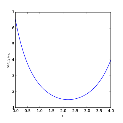
where denotes probabilities under a normal distribution with mean and variance . The standard deviation, the square root of the variance (4), is plotted for in Figure (1). The standard deviation has a single minimum, which is obtained for a value of which is close to , for which the mean of the tilted value coincides with the threshold. This basic example illustrates how importance sampling can lower dramatically the estimator variance.
As Fig. (1) shows, the relative error, which is proportional to the plotted quantity , can be reduced by a factor of more than for the case where . Since the error decreases as , this means a at least -fold longer brute force simulation would be necessary to obtain a similarly accurate result. For graphical purposes a relatively low threshold was chosen here. For higher thresholds, the performance gains increase drastically, with a reduction of computational effort by a factor when .
2.3 Genealogical particle analysis algorithm
The motivation for rare event simulation and the discussion of importance sampling have shown that it is necessary to make rare events less rare. This concept can be applied to stochastic processes such as the paths followed by either stochastic dynamics or chaotic deterministic dynamics. In those cases the objective is to alter the probability of certain paths that are connected to the rare event one wants to study.
Two different strategies are employed to alter the path sampling in stochastic dynamical systems. The first one is to alter the dynamical equations of the system by introducing a forcing term [41]. By tuning a parameter of the added forcing term, one can then attempt to decrease the variance of the rare event estimator. A second strategy consists in calculating an ensemble of realizations of the stochastic system in parallel and manipulating the ensemble members by performing selections at a finite number of selection times so as to bias the population.
Here we will use the second strategy, by employing a variant of the so called genealogical particle analysis algorithms. The selections applied to the ensemble consist of dynamical trajectories, called particles, being copied and killed depending on weight factor asigned to every ensemble member. This strategy has the advantage of not altering the dynamical trajectories themselves, such that their dynamics can be studied a posteriori.
Extensive analysis of the convergence of genealogical particle analysis algorithms can be found for example in [13, 14]. In the following sections, we perform a simpler calculation, assuming a mean field approximation, to demonstrate the evolution of the expected particle distributions in a genealogical particle analysis. The validity of this mean field approximation for large particle number is the subject of the complete proofs given in [13, 14]. Before going to a truly interacting genealogical particle analysis in Section 2.3.3, we first get some insight by looking at an algorithm where particles are reweighted, but by a factor depending only on the evolution of the particle itself, in Section 2.3.1.
2.3.1 A non-interacting genealogical particle analysis
We calculate rare events of a continuous time Markov chain. denotes the transition probabilities from configuration to over a time interval . We are interested in the probability of being in a set of configurations at a time , given that the process started in configuration at time . denotes the number of particles at time , whereas denote the particle configuration at time . denotes expectation values under the original Markov dynamics at time . The algorithm to generate the particles is described in the box “Algorithm 1”.
The algorithm can be summarized as follows: after initialization (step 1) the ensemble members are evolved forward in time (step 2a) and weight values are calculated from the previous and current configurations of the particle, and respectively (step 2b). Based on these weight values, ensemble members are killed or cloned (step 2c). Repeating this procedure results in a reweighted sample of paths, from which expectation values of the unweighted path distribution can be estimated (step 3). The rare event probability for a set can be obtained by taking as observable such that .
Note that the random number generated in step 2c can be zero, such that particles can be killed as well as cloned (when ). A way to generate the random number described in step 2c is to take where is uniformly distributed on and is the floor of (the largest integer smaller than ).
-
1.
Initiate particles in configuration :
-
2.
For every time step
-
(a)
Propagate under the dynamics, resulting in distributed according to with
-
(b)
Calculate weights for particle :
for a suitably chosen weight function
-
(c)
Generate a new particle distribution consisting of copies of particle with configuration where is chosen at random such that (note that )
-
(a)
-
3.
Finally, for any , calculate to estimate (to estimate take )
2.3.2 Unbiased estimator
We first show that Algorithm 1 provides an unbiased estimator for the quantity , i.e. the algorithm results in a random estimate whose expectation value equals the quantity to be estimated:
where is the expectation over the random variables in the algorithm.
Write the particle number at configuration , i.e. is the number of particles with :
According the algorithm 1, if a particle sits at at time step , copies are created of at the next time step. Hence, the particle number at the next time step will be
| (5) |
One step in the algorithm involves the generation of two sets of random variables, the updated particle configurations , which is conditioned on , and the number of particle copies , which depends on both and . The expectation value of functions depending on the particle configurations at step can therefore be expressed as the expectation value
Applying this expression to Eq. 5 and using the probabilities for the updated particle configurations and that the number of particle copies , we have
This equation relates the expected particle density at step to the density at step . By iteration we can relate the density at step to the density at the start of the algorithm, which is :
The expectation value of the quantity calculated at the end of the algorithm in step 3 is therefore
Note that the expected total particle number is in general not preserved over time. The particle number can strongly increase, which entails a large numerical cost. The solution to this problem is to renormalize the weights calculated in step 2b of the algorithm, hence introducing an interaction between the ensemble members. We discuss this new algorithm in the next section. As we will see, the interaction complicates the algorithm analysis.
2.3.3 Interacting particles
We now add interaction to the weights of the particle system, so as to control the particle number. A similar analysis as in the previous section can still be carried out, if one assumes that the number of particles used in algorithm is large enough, such that averages over particle configurations can be replaced by an expectation value under the law of large numbers (mean field approximation). The corresponding algorithm is described in the box “Algorithm 2”. By applying the algorithm to a function with the indicator function of the set , estimates of the probability can be obtained.
-
1.
Initiate particles in configuration ,
-
2.
For every time step
-
(a)
Propagate under the dynamics, resulting in distributed according to with
-
(b)
Calculate weights for particle :
-
(c)
Store the value of the normalizing factor
-
(d)
Generate a new particle distribution consisting of copies of particle with configuration where is chosen at random such that
-
(a)
-
3.
Finally calculate to estimate (for take )

We again perform an analysis of the evolution of the expected particle distribution in Algorithm 2. For simplicity of the derivation we assume that the number of particles in the algorithm is large, such that by the law of large numbers,
| (6) | |||||
| (7) |
Using this estimate and the same reasoning as for the non-interacting particle algorithm, we have for the expected particle distribution that
| (8) |
The expectation value of in the denominator can be substituted using Eq. 6. The particle number is now constant:
We therefore have that
Inserting this into 8, we have
Therefore by iteration
The above reasoning can also be extended to show that path dependent quantities (such as for ) can be estimated from the ancestral paths of the particle system.
2.3.4 Time-dependent weighting
The weighting function results in a particle distribution tilted by at all selection times . More flexibility can be obtained by using time-dependent weighting, for example with a weighting function of the form
| (9) |
This way the telescoping canceling of is preserved in products of weights that appear in the calculation of the tilted measure. For example,
The result is again a particle distribution tilted by at time , as with the time-independent weight function. However, paths up to the final time will have different weights, which can make a large difference in the algorithm performance, as we will demonstrate in Section 4.2.4.
3 Fluctuation paths and the weighting function
The ideal change of measure discussed in Section 2.2 suggests to make the rare event that is the least rare the most probable one under the reweighted dynamics. This rationale extends not only to the distribution of the system at the final time, but also to the entire path up to the final time. This means that variance can be reduced if the least unlikely path leading to a high threshold is made more likely under the particle system dynamics.
For stochastic differential equations in the weak noise limit, the least unlikely path from an attractor can be calculated from Freidlin-Wentzell type large deviation theory and is called a fluctuation path (also sometimes an instanton). The particle system dynamics can be made to more closely follow the fluctuation path by using the time-dependent weighting discussed in Section 2.3.4. Even if the particle distribution at the final time is the same as the particle distribution obtained with a constant weighting, there is still a variance reduction since less particles are killed, increasing the independence of the particle and thus the effective particle number.
3.1 Fluctuation paths
The probability of a given path in a stochastic differential equation with small noise,
where is a Brownian motion, can be estimated using the Freidlin-Wentzell large deviation theory. The theory determines the probability of seeing a path that is close to a specified continuous function in the limit of going to zero. It roughly states that
where is any closed subset of the set of continuous trajectories and the rate functional is called the action. The action is given by
| (10) | |||
| (11) |
The distribution of paths leading to rare fluctuations then concentrates around action minima as decreases, with given constraints. If the set of paths contains the evolution along the deterministic dynamics , this path will obviously minimize the above action, hence the need for constraints to obtain more interesting results. For example, in the simple case were the deterministic dynamics has a single attractor , the distribution of the paths conditioned on concentrate close to the minima of the action with the boundary conditions and . Such a path is called a fluctuation path leading to (it is also sometimes called an instanton, but instanton usually rather refers to those fluctuation paths that connect attractors to saddle points).
4 Rare event simulation for a stochastic process: the Ornstein-Uhlenbeck process
We now illustrate some of the practical issues arising when implementing a genealogical particle analysis algorithm for rare event estimation. We start off with a stochastic process for which we can calculate explicitly all of the probabilities that we want to estimate, for pedagogical reasons, and so that we can compare the numerical results to the analytic expressions.
4.1 Description of the Ornstein-Uhlenbeck process
We consider the Ornstein-Uhlenbeck process
| (12) |
As the transition probabilities are Gaussian, the Ornstein-Uhlenbeck process preserves Gaussianity. Using the Itô formula, one can derive that the mean and the variance evolve according to the equations
| (13) |
which can be easily solved explicitly.
The probability that exceeds a certain threshold at a time , given that the process started at at time zero can be calculated explicitly as
| (14) |
where and solve (13) and is the probability density function of the normal distribution with mean and variance . We consider in the following the estimation of this probability through a genealogical particle analysis algorithm. Below we will use the parameter values and .
4.2 Algorithm implementation
Let us assume we seek to estimate a small probability , for instance . We denote the number of particles for each realization of the algorithm. Then each independent realization of the algorithm, with particle each, will give an estimate . According to a theorem discussed in [19], asymptotically for large , the random number is distributed according to a Gaussian distribution with standard deviation and a corresponding relative error . The value of the estimator relative error is essential as it quantifies the relative error one should expect for each realization of the algorithm, and thus the quality of the result. How the estimator relative error depends on the number of selections, on their timing, and the type observables are critical questions that we analyze in this section.
4.2.1 Number of particles
The result in [19] proves the existence of the central limit theorem, but does not give a value for the estimator variance . In order to get an estimate of , we compute it empirically by performing independent algorithm realization and using the estimator
| (15) |
In this formula the value of will be either the theoretical
value when it is available, for instance for the Ornstein-Uhlenbeck
process, or the estimated value of the probability by averaging
over realizations. In the following, by an abuse of notation,
denotes either the theoretical estimator variance of the estimator
variance evaluated from (15), which one should
be clear from the context.
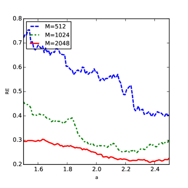
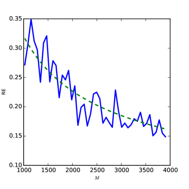
We first study the estimator variance for the Ornstein–Uhlenbeck case. We first test whether or not the regime of the central limit theorem has been reached by changing the number of particles , and verifying whether (15) reduces by the corresponding factor. Figure 3a shows the expected decrease in relative error as the number of particles is increased for a range of thresholds (see eq. (14)). The inverse square root behavior of the error with increasing number of particles is demonstrated for a fixed threshold in Figure 3b. The parameters are specified in the figure captions.
We study how the estimator variance depends on the other numerical parameters in the following sections.
4.2.2 Number of selections and their timing
Since little theoretical analysis has been performed on the optimal number of selection steps, this is the most heuristic choice to be made. Some numerical analysis of this issue has been performed in [42]. For the problem they investigate, changing the number of selections, and using equidistant in time selections, the estimator variance clearly shows a minimum for a certain number of selections.
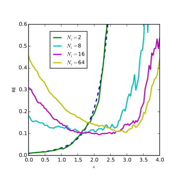
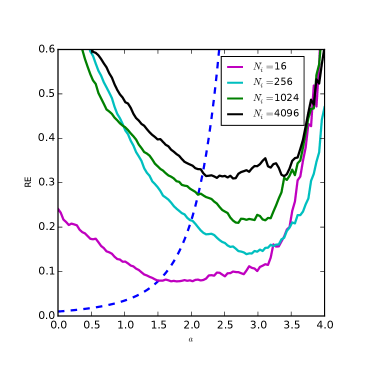
This result can be interpreted as follows. Selections shouldn’t be performed too frequently, as cloning increases correlations between the particles and therefore reduces the effective number of independent particles, increasing the estimator variance. If not performing selections frequently enough however, the particle distribution relaxes to the unbiased particle measure, leading to the poor brute force Monte-Carlo variance. This can be seen in Figure 4: for low thresholds , importance sampling is useless and estimations with a small number of selections have the lowest estimator relative error . Due to the large time between selections, the particles have relaxed to the particle measure of brute force Monte Carlo simulations and therefore have a similar estimator variance. For higher thresholds, for instance for , it becomes advantageous to kill a larger number of particles to obtain a more skewed final particle distribution, in order to lower the variance. For the threshold value the optimal number of interactions among the values in the figure is . For higher thresholds there is a small reduction in error by increasing the number of selections, although increasing the number of selections much further beyond results in an overall increase of error.
Figure 4 also illustrates the large estimator
variance improvement for the genealogical particle analysis algorithm
compared with Monte-Carlo sampling, as soon as .
Besides the number of selections, there also seems to be little theoretical understanding of the optimal timing for selections. One strategy to selection timing is to calculate on-the-fly a criterion on the distribution of particle weights (such as the squared coefficient of variation or entropy) and only perform selection if a fixed threshold is exceeded. The convergence of such adaptive selection strategies is discussed in [43].
4.2.3 Estimating a range of over-threshold probabilities
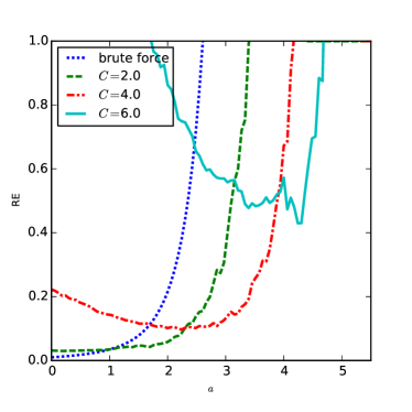
In the following the weight function is used. From the point of view of the estimator variance (15), to each value of the threshold corresponds an optimal value of , denoted , or equivalently for each value of the estimator variance has a minimum for a given value of , denoted . For instance Figure 4 shows that the value is optimal for . In simple cases, we expect to increase monotonically with .
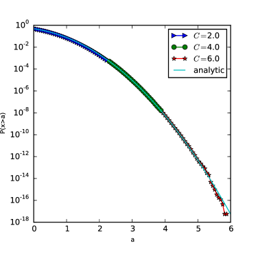
There is an optimal value of for each value of , however the estimate is good for a range of thresholds around this optimum. When instead of a particular over-threshold probability one is interested in the tail of the complete distribution probability, one can perform a number of genealogical particle analysis simulations each with different value of , and select for each threshold the value corresponding to the lowest estimator variance . Figure 5 illustrates how the tail of can be estimated this way, for the Ornstein-Uhlenbeck process. For large values of the threshold (above ) all estimates have a high error and the highest value of is chosen by default. As can be seen on this figure there is very good agreement with the theoretical value up to probabilities as low as . Using this strategy, we can accurately estimate the tail of the over-threshold distribution down to probabilities as small as , with relative error lower than one.
4.2.4 Selections along the fluctuation paths
We have discussed in Section 2.3.4 that a time-dependent weighting function can be used. In this way the particle distribution can be weighted with different exponential factors all along the path, but still lead to the same exponentially tilted final particle distribution. Furthermore, in Section 3.1 we have discussed how for small noises, most of the paths leading to a rare event will concentrate around fluctuation paths that minimize the action functional. The aim of this section is to demonstrate the interest of using fluctuation paths to construct time-dependent weighting functions in order to increase the efficiency of the genealogical particle analysis algorithm.
Since the Ornstein-Uhlenbeck process is linear, taking limits of higher thresholds is equivalent to taking a weak-noise limit through a rescaling of the coordinate. Hence, for fixed noise intensity , paths starting at conditioned on reaching the final threshold will concentrate around the fluctuation paths in the limit . The action (10) for the Ornstein-Uhlenbeck process (12) is given by . Taking as boundary conditions and the fluctuation paths are easily computed to be
By using the potential function with a weight parameter dependent on the selection time , we can control , the mean particle position at , by fixing . The expected particle distribution for the Ornstein-Uhlenbeck process tilted with this weighting function after the selection at is
as discussed in Section 2.3.4. The corresponding expected mean particle position is therefore where is the variance of the Ornstein-Uhlenbeck process at time (the solution of Eq. 13 with ). Choosing , follows and the algorithm particle distribution closely follows the fluctuation path leading to the threshold .
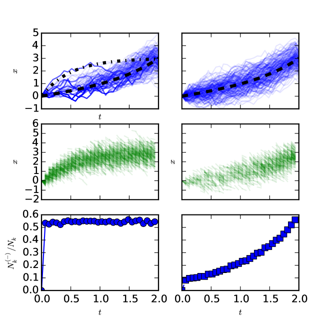
Figure 6 shows the effect of using a weight function based on a fluctuation path versus an exponential weight function. The bottom two plots show how using the fluctuation path significantly decreases the fraction of particles that are killed during the selection steps () to the number of particles at that time step (). This is also illustrated in the plots in the top and middle rows. The top plots show the paths from the initial state for all surviving particles at the final time. Paths that have been killed during the process are not shown. We call these paths the ancestral paths. As can be seen on the top left plot, only few trajectories from the initial stage of the algorithm are ancestors of the final positions. This is not the case for the top right plot. The algorithm using a weight based on a fluctuation path has a much larger number of ancestors. This richer ancestral tree results in a decreased estimator error for the over-threshold probabilities, as is demonstrated in Figure 7.
Note that for both the exponential weighting function and the weighting based on the fluctuation path, the paths reaching the threshold follow the fluctuation path. Other paths reaching the threshold are so rare that few of them are generated, even if they are more likely to survive selection in the case of exponential weighting. Note that the killed paths, partially shown in the middle row of Fig. 6, tend to have a negative change in position before being killed. The higher target path in the exponential makes for a higher average dissipative force on the particles, leading to a large discrepancy between the actual particle distribution and the target distribution at selection times.
5 Genealogical particle analysis algorithm for a deterministic dynamical system: the Lorenz ’96 model
The Lorenz ’96 model is a deterministic dynamical system that is often used as a toy model in the meteorology community. It was proposed by Lorenz as part of a study on error growth and predictability for chaotic dynamical systems [39, 40].
A crucial difference between the famous Lorenz ’63 model and the less well-known Lorenz ’96 model is that the latter has a large number of degrees of freedom. Indeed macroscopic variables of deterministic systems with a large number of degrees of freedom often behave qualitatively similar to solutions of stochastic differential equations with much less degrees of freedom. Such results can be proven for some specific types of models (feauturing separation of time scale, independence, …).
It is believed however that similar results remain true for a wide range of models and observables even though mathematical proofs are out of reach. If this conjecture is correct, then the sampling of rare events through genealogical particle analysis algorithms should be applicable to macroscopic variables of deterministic systems with a large number of degrees of freedom. In this section, we demonstrate empirically, through numerical simulation, that genealogical particle analysis algorithms can indeed efficiently sample the tail of the energy distribution for the Lorenz ’96 model.
5.1 Description of the model
The Lorenz ’96 model consists of variables on a ring , with dynamics
where indices are in , i.e. the index is identified with if . The non-linear part of the dynamics conserves the energy , while is a forcing and a linear dissipation. The dynamics is chaotic for [39, 40]. We will estimate the probability of reaching a certain energy threshold after a time , starting from the zero vector . A small perturbation is added to the particle configuration to make the trajectories diverge. For large enough times , the system will therefore relax to its physical invariant measure and it makes sense to determine probabilities of exceedances of macroscopic observables . Throughout the article we will use a number of variables and a forcing .
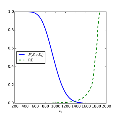
Figure 8 shows a plot of the over-threshold probabilities of the energy of the Lorenz ’96 system, estimated through a brute force Monte-Carlo simulation from randomly perturbed initial conditions. Given that we have finite computer resources at our disposal, assume we can generate at most independent measurements of the energy. If the maximal relative error that we are willing to tolerate is for example then since the lowest probability that we can estimate is approximately . From Figure 8 we can deduce that the corresponding highest energy threshold obtainable lies around an energy threshold . Beyond this threshold the use of rare event algorithms becomes necessary.
5.2 Algorithm implementation
We use the following settings for the genealogical particle analysis simulation. The initial condition is set to . The total integration time per realization is . This time interval corresponds to roughly times the decorrelation time of the energy observable. The standard deviation of the estimator is estimated from independent runs of the algorithm and the truth is taken from a long brute force Monte Carlo simulation. The number of interaction is set to .
5.2.1 Weight function
For simplicity, we have employed an exponential weight function where is the change in energy between two interactions. This choice doesn’t require any a priori knowledge of the dynamics and is easy to implement. This weight function is not optimal, but, as we will show, it already gives good results.
For the value of the forcing parameter the distribution of the energy values is roughly Gaussian. One can therefore estimate the mean and the variance from a brute force Monte Carlo simulation and use these values along with the reasoning of Section 2.2.1 to determine an appropriate value of the exponential weighting factor in the weighting function . One can then choose a value where is the desired change of the mean energy of the final particle distribution.
The values of in the weighting function for the calculations presented in this section are taken as with and being the standard deviation of the energy so as to increase the mean energy by steps of size .
5.2.2 Noise perturbation
For deterministic dynamical systems, in order for two trajectories to have different dynamics after selection, a small perturbation can be added. This can be achieved by adding for example a weak Brownian perturbation at all times, or by adding a small instantaneous perturbation to offspring at the selection times. The former approach provides a simpler mathematical framework. Indeed the study of the noise effect would amount to the study of the stochastic differential equation properties in the weak noise limit, independent of the genealogical particle analysis algorithm. By contrast the latter approach intertwines the random perturbation with the genealogical particle analysis algorithm effects and is therefore more complicated to analyze. The latter approach, however, has the practical advantage of being computationally simpler. In this study, as we will proceed purely empirically, we have opted for the latter approach. The clones are perturbed by where is a standard -dimensional Gaussian random variable, i.e. the noise acts independently on all of the variables.
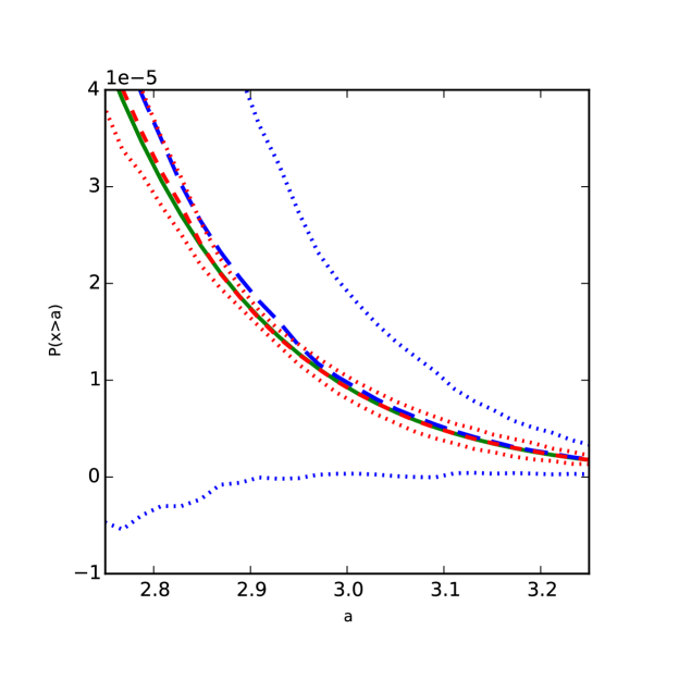
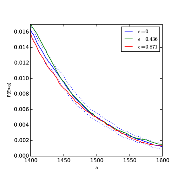
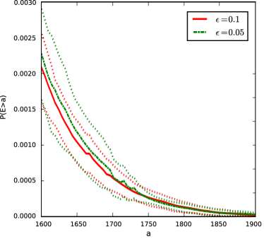
The small noise perturbation invariably adds an error to the estimates of the tail probabilities. To obtain a rough upper bound on the strength of the perturbation that can be added without significantly perturbing the tail, we first perform a brute force simulation with the added noise for different noise strengths and verify that the tail probabilities do not change significantly compared to the sampling error of the brute force calculation. A set of independent realizations is performed like in the brute force Monte Carlo approach, the only difference being that at the selection times the same noise perturbations is added as in the genealogical particle analysis simulation. No selection is performed however in these runs. This way we can estimate the effect of the noise on the final time particle distribution. Figures 9a and 9b show that below a perturbation strength of and for thresholds higher than , the noise does not have a significant effect on the over-threshold probabilities. More complex schemes of noise perturbation could be implemented to assure that the perturbed trajectory remains close to the attractor, for example by storing a configuration at a time point before , adding a small perturbation to it and evolve it up to to have the perturbation relax towards the attractor.
Furthermore, after performing the genealogical particle analysis algorithm, we check that the perturbing noise intensity is small enough by decreasing and checking that the estimates of the over-threshold tail statistics are consistent. Figure 9b shows that for the results remain stable upon halving the noise intensity.
5.2.3 Estimating the tail of the energy distribution
We use for the Lorenz ’96 model the procedure described in Section 4.2.3: we increase the values of the weight parameter and use for each threshold value the best estimate from the point of view of the empirical estimator variance. The result is shown in Figure 10. As there is no analytic expression for the energy distribution tail of the Lorenz ’96 system, we use a long brute force Monte Carlo estimation as comparison. The estimator variance markedly decreases when using the genealogical particle analysis algorithm. When constructing the over-threshold probability, we see that the tail can be reliably reproduced when compared to the longer brute force calculation.
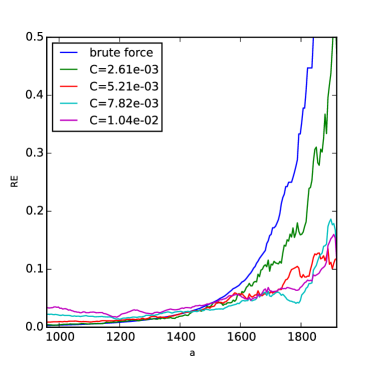
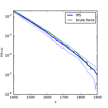
The improvements in efficiency from using a rare event simulation scheme can be quantitatively estimated from Figure 10. The plot of the empirical relative error shows how for a threshold around a brute force Monte Carlo calculation yields a relative error of , whereas the genealogical particle analysis simulation yields a relative error of approximately . A reduction in relative error by a factor is achieved. Since the brute force Monte Carlo error scales as , a similar reduction by a raw increase of processing power would require to increase by a factor of . For higher thresholds and with more fine tuning of the selection process, a much larger reduction is likely to be achievable.
6 Conclusion
In this paper we have addressed the use of rare event computation techniques to estimate small over-threshold probabilities of observables in deterministic dynamical systems. We have demonstrated that the genealogical particle analysis algorithms can be successfully applied to a toy model of atmospheric dynamics, the Lorenz ’96 model as presented in Section 5.1. We have furthermore used the Ornstein-Uhlenbeck system to illustrate a number of implementation issues.
The example of the Ornstein-Uhlenbeck has illustrated the importance of the choice of the objective function for the performance of the genealogical particle analysis algorithm estimator. We have shown how a time-dependent objective function based on the fluctuation path to a high threshold can greatly improve the performance of the estimator compared to a fixed-in-time objective function. Furthermore we have discussed how the number of particles and the number of selection steps influence the performance of the estimator.
For the deterministic chaotic system a complication arises in that a stochastic perturbation needs to be added to the system to make identical clones of one parent diverge and explore the system’s path space. We have demonstrated in this example how the estimates of the rare event simulation are stable for small perturbations and agree with results from brute force Monte Carlo estimations. We therefore can have confidence in the correctness of these estimates.
For the example of a deterministic chaotic system that we have studied we have not yet used the fluctuation path approach, since this would require information on the dynamics to the rare event that we a priori do not possess. This lack of knowledge can be improved by iterating the estimation procedure, where one uses estimates of an initial brute force simulation to estimate the fluctuation path, after which an genealogical particle analysis simulation based on this path can be used to estimate a higher fluctuation path, which can be used for a next iteration of the algorithm. However, the results of the straightforward implementation of the rare event simulation already shows significant improvements compared to brute force estimation.
Acknowledgements
The authors would like to thank Eric Vanden-Eijnden, Eric Simonnet, Joran Rolland, Pascal Yiou, Bérengère Dubrulle, Francesco Ragone and Takahiro Nemoto for fruitful discussions.
JW acknowledges the support of the AXA Research Fund.
The research leading to these results has received funding from the European Community’s Seventh Framework Programme (FP7/2007-2013) under grant agreement n° PIOF-GA-2013-626210.
References
- [1] Qiu B and Miao W 2000 Journal of Physical Oceanography 30 2124–2137 ISSN 0022-3670
- [2] Schmeits M J and Dijkstra H A 2001 Journal of Physical Oceanography 31 3435–3456 ISSN 0022-3670
- [3] Glatzmaier G A and Roberts P H 1995 Physics of the Earth and Planetary Interiors 91 63–75 ISSN 0031-9201
- [4] Intergovernmental Panel on Climate Change 2012 Managing the risks of extreme events and disasters to advance climate change adaption: special report of the Intergovernmental Panel on Climate Change (New York, NY: Cambridge University Press) ISBN 978-1-107-02506-6
- [5] Barriopedro D, Fischer E M, Luterbacher J, Trigo R M and García-Herrera R 2011 Science 332 220–224 ISSN 0036-8075, 1095-9203
- [6] Wetter O and Pfister C 2013 Clim. Past 9 41–56 ISSN 1814-9332
- [7] de Haan L 2006 Extreme value theory: an introduction Springer series in operations research (New York ; London: Springer) ISBN 0-387-23946-4
- [8] Leadbetter M R 1983 Extremes and related properties of random sequences and processes Springer series in statistics (New York: Springer-Verlag) ISBN 0-387-90731-9
- [9] Kharin V V and Zwiers F W 2005 Journal of Climate 18 1156–1173 ISSN 0894-8755
- [10] Kyselý J 2002 Studia Geophysica et Geodaetica 46 93–112 ISSN 0039-3169, 1573-1626
- [11] Rubino G and Tuffin B (eds) 2009 Rare event simulation using Monte Carlo methods (Chichester, UK: Wiley) ISBN 978-0-470-77269-0
- [12] Bucklew J A 2004 An introduction to rare event simulation (New York: Springer) ISBN 0-387-20078-9 978-0-387-20078-1 1-4419-1893-0 978-1-4419-1893-2
- [13] Del Moral P 2013 Mean field simulation for Monte Carlo integration ISBN 978-1-4665-0417-2 1-4665-0417-X
- [14] Del Moral P 2004 Feynman-Kac Formulae Genealogical and Interacting Particle Systems with Applications (New York, NY: Springer New York) ISBN 978-1-4684-9393-1 1-4684-9393-0
- [15] Cérou F and Guyader A 2007 Stochastic Analysis and Applications 25 417–443 ISSN 0736-2994
- [16] Rolland J, Bouchet F and Simonnet E 2015 Computing transition rates for the 1-D stochastic Ginzburg-Landau-Allen-Cahn equation for finite-amplitude noise with a rare event algorithm
- [17] Rolland J and Simonnet E 2015 Journal of Computational Physics 283 541–558 ISSN 0021-9991
- [18] Heymann M and Vanden-Eijnden E 2008 Communications on pure and applied mathematics 61 1052–1117
- [19] Del Moral P and Garnier J 2005 The Annals of Applied Probability 15 2496–2534 ISSN 1050-5164
- [20] Garnier J and Moral P D 2006 Optics Communications 267 205–214 ISSN 0030-4018
- [21] Hairer M and Weare J 2014 Communications on Pure and Applied Mathematics 67 1995–2021 ISSN 1097-0312
- [22] Tailleur J and Kurchan J 2007 Nature Physics 3 203–207 ISSN 1745-2473 wOS:000244558400021
- [23] Laffargue T, Lam K D N T, Kurchan J and Tailleur J 2013 Journal of Physics A: Mathematical and Theoretical 46 254002 ISSN 1751-8121
- [24] Giardinà C, Kurchan J, Lecomte V and Tailleur J 2011 Journal of Statistical Physics 145 787–811 ISSN 0022-4715, 1572-9613
- [25] Lecomte V and Tailleur J 2007 Journal of Statistical Mechanics: Theory and Experiment 2007 P03004 ISSN 1742-5468
- [26] Giardinà C, Kurchan J and Peliti L 2006 Physical Review Letters 96 120603
- [27] Kurchan J 2015 Physica A: Statistical Mechanics and its Applications 418 170–188 ISSN 0378-4371
- [28] Vanden-Eijnden E and Venturoli M 2009 The Journal of chemical physics 131 044120
- [29] Adams D A, Sander L M and Ziff R M 2008 Physical Review Letters 101 144102
- [30] Chandler D 2005 Nature 437 640–647 ISSN 0028-0836
- [31] Noé F, Schütte C, Vanden-Eijnden E, Reich L and Weikl T R 2009 Proceedings of the National Academy of Sciences 106 19011–19016 ISSN 0027-8424, 1091-6490
- [32] Metzner P, Schütte C and Vanden-Eijnden E 2006 The Journal of Chemical Physics 125 084110 ISSN 0021-9606, 1089-7690
- [33] Bolhuis P G, Chandler D, Dellago C and Geissler P L 2002 Annual Review of Physical Chemistry 53 291–318
- [34] Wolde P R t and Frenkel D 1997 Science 277 1975–1978 ISSN 0036-8075, 1095-9203
- [35] E W, Ren W and Vanden-Eijnden E 2003 Journal of Applied Physics 93 2275–2282 ISSN 0021-8979, 1089-7550
- [36] Kohn R V, Reznikoff M G and Vanden-Eijnden E 2005 Journal of Nonlinear Science 15 223–253 ISSN 0938-8974, 1432-1467
- [37] Grafke T, Grauer R and Schäfer T 2013 Journal of Physics A: Mathematical and Theoretical 46 062002
- [38] Grafke T, Grauer R, Sch fer T and Vanden-Eijnden E 2014 Multiscale Modeling & Simulation 12 566–580
- [39] Lorenz E N 1996 Predictability: A problem partly solved GARP Publication Series vol 16 (Geneva, Switzerland: WMO) pp 132–136
- [40] Lorenz E N 2005 Journal of the Atmospheric Sciences 62 1574–1587 ISSN 0022-4928, 1520-0469
- [41] Vanden-Eijnden E and Weare J 2012 Communications on Pure and Applied Mathematics 65 1770–1803 ISSN 1097-0312
- [42] El Makrini M, Jourdain B and Lelièvre T 2007 ESAIM: Mathematical Modelling and Numerical Analysis 41 189–213
- [43] Del Moral P, Doucet A and Jasra A 2012 Bernoulli 18 252–278 ISSN 1350-7265