Probing non-perturbative effects in M-theory on orientifolds

Abstract

Using holography, we study non-perturbative effects in M-theory on orientifolds from the analysis of the $S^{3}$ partition functions of dual field theories. We consider the $S^{3}$ partition functions of $\mathcal{N}=4$ Yang-Mills theory with $O(n)$ gauge symmetry coupled to one (anti)symmetric and $N_{f}$ fundamental hypermultiplets from the Fermi gas approach. In addition to the worldsheet instanton and membrane instanton corrections to the grand potential, which are also present in the $U(n)$ Yang-Mills case, we find that there exist “half instanton” corrections coming from the effect of orientifold plane.

1 Introduction

In the last few years, we have witnessed a tremendous progress in our understanding of non-perturbative effects in M-theory. In particular, in the case of $\mathcal{N}=6$ $U(N)_{k}\times U(N)_{-k}$ ABJM theory, which is holographically dual to M-theory on $AdS_{4}\times S^{7}/\mathbb{Z}_{k}$, we have a complete understanding of non-perturbative corrections thanks to the relation to topological string on local $\mathbb{P}^{1}\times\mathbb{P}^{1}$ HMMO (see Hatsuda:2015gca for a review). Especially, the grand partition functions of ABJM theory at $k=1,2,4$ are completely determined in closed forms Codesido:2014oua ; Grassi:2014uua .

However, for lower supersymmetric theories we still do not have a detailed understanding of non-perturbative effects in M-theory. $d=3~{}\mathcal{N}=4$ theories are particularly interesting since these theories are sometimes related by mirror symmetry exchanging the Higgs branches and Coulomb branches Intriligator:1996ex . Such $\mathcal{N}=4$ theories naturally appear as the worldvolume theories on M2-branes probing ALE singularities. For instance, $N$ M2-branes probing $A_{N_{f}-1}$ ALE singularities have two descriptions related by mirror symmetry: $U(N)$ Yang-Mills theory with one adjoint and $N_{f}$ fundamental hypermultiplets, and a $\widehat{A}_{N_{f}-1}$ quiver gauge theory Intriligator:1996ex ; deBoer:1996mp . The former theory appears as a worldvolume theory on $N$ D2-branes in the presence of $N_{f}$ D6-branes, and the latter description comes from the M-theory lift of D6-branes as Taub-NUT space. In the large $N$ limit, these theories are holographically dual to M-theory on $AdS_{4}\times S^{7}/\mathbb{Z}_{N_{f}}$, and we can study non-perturbative effects in this background from the $S^{3}$ partition function of the field theory side. In Mezei:2013gqa ; GM ; Hatsuda:2014vsa , the $S^{3}$ partition function of these theories, known as the $N_{f}$ matrix model, are studied using the Fermi gas formalism MP2 . It turned out that the instanton corrections in the $N_{f}$ matrix model are quite different from those in the ABJM theory and have a very intricate structure Hatsuda:2014vsa . Instanton corrections in more general $\mathcal{N}=4$ quiver gauge theories are also studied in Moriyama:2014waa ; Moriyama:2014nca ; Hatsuda:2015lpa , but it is fair to say that we are far from the complete picture.

In this paper, we will study a natural generalization of $N_{f}$ matrix model: $S^{3}$ partition functions of $d=3~{}\mathcal{N}=4$ $O(n)$ or $USp(n)$ Yang-Mills theories with $N_{f}$ fundamental and one (anti)symmetric hypermultiplets, first studied in Mezei:2013gqa using the Fermi gas approach. In the Type IIA brane constructions, such models appear as worldvolume theories on $N$ D2-branes in the presence of $N_{f}$ D6-branes and a orientifold plane. We will denote the model of gauge group $G$ with $N_{f}$ fundamental and one symmetric (or anti-symmetric) hypermultiplets as $G+S$ (or $G+A$), respectively.

By mirror symmetry, the $USp(2N)+A$ model is dual to a $\widehat{D}_{N_{f}}$ quiver gauge theory Intriligator:1996ex ; deBoer:1996mp , which can be interpreted as the worldvolume theory on M2-branes probing the $D_{N_{f}}$ ALE singularity. In the large $N$ limit, this theory is holographically dual to M-theory on $AdS_{4}\times S^{7}/\Gamma_{D_{N_{f}}}$ where $\Gamma_{D_{N_{f}}}$ is the dihedral subgroup of $SU(2)$. This opens up an avenue to study M-theory on orientifolds from the analysis of $S^{3}$ partition functions of dual field theories. In particular, we can study the effects of orientifold plane in the M-theoretic regime where the string coupling $g_{s}$ of Type IIA theory becomes large. Orientifolds in Type IIB theory can be described in F-theory, while the strong coupling behavior of Type IIA orientifolds is still poorly understood. Our work is a first step towards the understanding of non-perturbative effects in M-theory on orientifolds.

We find that the $USp(n)+A$(or $S$) model is related to the $O(n)+A$(or $S$) model by a shift of $N_{f}$, hence it is sufficient to consider the $O(n)$ case only. For the $O(n)+A$ model we find that there are three types of instantons: worldsheet instantons, membrane instantons, and “half instantons”. The first two types have direct analogues in the $N_{f}$ matrix model, while the last type is a new one coming from the effect of orientifold plane. In the Fermi gas picture, orientifolding corresponds to the reflection of fermion coordinate $x\to-x$, and the “half instantons” can be naturally identified as the contribution of the twisted sector of this reflection. We find that the sign of this contribution depends on the parity $(-1)^{n}$ of the gauge group $O(n)$. On the other hand, we could not find a clear picture of the instanton corrections in the $O(n)+S$ model.

This paper is organized as follows:

In section 2, we first review the Fermi gas formalism of the $S^{3}$ partition functions of $G+A$ or $G+S$ models Mezei:2013gqa . Then we explain our algorithm to compute the partition functions of these models exactly.

In section 3, we determine the coefficients $C,B$ and $A$ in the perturbative part of grand potential (14). The results are summarized in Table 2.

In section 4, we study the non-perturbative corrections to the grand potential using our data of exact partition functions. For the $O(n)+A$ model, we find the first few coefficients of instanton corrections as a function of $N_{f}$. We also comment on the instanton corrections in the $O(n)+S$ model.

In section 5, we compute the WKB expansion of grand potential using the density matrix operator in Assel:2015hsa , and reproduce the coefficients $C,B$ and $A$ for the $O(2N+1)+A$ model.

In section 6, using the different form of operator in Mezei:2013gqa , we compute the WKB expansion of the “twisted spectral trace” defined in (87). We argue that this contribution is related to the effect of orientifold plane.

Finally, we conclude in section 7. Additionally, we have two Appendices A and B. In Appendix A, we summarize the non-perturbative part of grand potential $J_{\text{np}}(\mu)$ for various (half-)integer $N_{f}$, determined from our data of exact partition functions. In Appendix B, we explain the derivation of the Wigner transform in (55).

2 Fermi gas formalism and exact computation of partition functions

We study the $S^{3}$ partition functions of $\mathcal{N}=4$ $G+A$ and $G+S$ models with $G=O(n)$ or $USp(n)$, considered previously in Mezei:2013gqa . Such models naturally appear as worldvolume theories on D2-branes in the presence of $N_{f}$ D6-branes and a orientifold plane.

As discussed in Mezei:2013gqa , depending on the type of orientifold plane, we find the following models as worldvolume theories on D2-branes:

• $O(2N)+A$: $N$ D2-branes and $N_{f}$ D6-branes with a O2^- plane.

• $O(2N+1)+A$: $N$ D2-branes and $N_{f}$ D6-branes with a O2^- plane on which a half D2-brane got stuck.

• $O(2N)+S$: $N$ D2-branes and $N_{f}$ D6-branes with a O6⁺ plane.

• $O(2N+1)+S$: $N$ D2-branes and $N_{f}$ D6-branes with a O6⁺ plane on which a half D2-brane got stuck.

• $USp(2N)+A$: $N$ D2-branes and $N_{f}$ D6-branes with a O6^- plane.

• $USp(2N)+S$: $N$ D2-branes and $N_{f}$ D6-branes with a O2⁺ plane.

To preserve $\mathcal{N}=4$ supersymmetry, we consider a configuration of D2-branes and O2-planes extending in the directions $(x^{0},x^{1},x^{2})$, and D6-branes and O6-planes extending in the directions $(x^{0},x^{1},\cdots,x^{5})$ Mezei:2013gqa . They share the common three dimensional spacetime $(x^{0},x^{1},x^{2})$ on which the above $d=3~{}\mathcal{N}=4$ theories live.

In Mezei:2013gqa , it is found that the $S^{3}$ partition functions of above models can be written as a system of $N$ fermions in one-dimension ($x_{i}\in\mathbb{R}$)

$$Z(N,N_{f}) =\frac{1}{N!}\int\frac{d^{N}x}{(4\pi)^{N}}\prod_{i=1}^{N}\frac{(2\sinh\frac{x_{i}}{2})^{2a}(2\sinh x_{i})^{2b}(2\cosh x_{i})^{1-2d}}{(2\cosh\frac{x_{i}}{2})^{2N_{f}+2c}}\det\left(\frac{1}{2\cosh x_{i}+2\cosh x_{j}}\right)$$ (1)

$$=\frac{1}{N!}\sum_{\sigma\in S_{N}}(-1)^{\sigma}\int d^{N}x\prod_{i=1}^{N}\rho(x_{i},x_{\sigma(i)}),$$

where the density matrix $\rho(x,y)$ is given by

$$\rho(x,y) =\frac{\sqrt{V(x)V(y)}}{2\cosh x+2\cosh y},$$ (2)

$$V(x) =\frac{1}{4\pi}\frac{(2\sinh\frac{x}{2})^{2a}(2\sinh x)^{2b}(2\cosh x)^{1-2d}}{(2\cosh\frac{x}{2})^{2N_{f}+2c}}.$$

The parameters $a,b,c,d$ for each model are summarized in Table 1.

model	$a$	$b$	$c$	$d$
$O(2N)+A$	0	0	0	0
$O(2N+1)+A$	1	0	1	0
$O(2N)+S$	0	0	0	1
$O(2N+1)+S$	1	0	1	1
$USp(2N)+A$	0	1	0	0
$USp(2N)+S$	0	1	0	1

Table 1: $a,b,c,d$ for various models

In (1), we have fixed the overall normalization of $Z(N,N_{f})$ in such a way that $Z(N=0,N_{f})=1$, which is a natural normalization in the Fermi gas formalism MP2 . Note that our normalization of $Z(N,N_{f})$ is different from Mezei:2013gqa . As discussed in MP2 , to study the non-perturbative corrections, it is more convenient to consider the grand partition function by summing over $N$ with fugacity $e^{\mu}$

$$\Xi(\mu)=\sum_{N=0}^{\infty}Z(N,N_{f})e^{N\mu}.$$ (3)

From (1), one can show that $\Xi(\mu)$ can be written as a Fredholm determinant of the density matrix $\rho$

$$\Xi(\mu)=\text{Det}(1+e^{\mu}\rho).$$ (4)

More physically, $\rho$ is identified with the Hamiltonian $H$ of the fermion system as

$$\rho=e^{-H}.$$ (5)

In the following sections, we will study the large $\mu$ expansion of the grand potential $J(\mu)$

$$J(\mu)=\log\Xi(\mu)=\sum_{\ell=1}^{\infty}\frac{(-1)^{\ell-1}e^{\ell\mu}}{\ell}\operatorname{Tr}(\rho^{\ell}).$$ (6)

From (1) and Table 1, one can easily see that the partition functions of $USp(2N)$ theory and $O(2N+1)$ theory are related by a shift of $N_{f}$

$$Z(N,N_{f})_{USp(2N)+A} =Z(N,N_{f}-2)_{O(2N+1)+A},$$ (7)

$$Z(N,N_{f})_{USp(2N)+S} =Z(N,N_{f}-2)_{O(2N+1)+S}.$$

Therefore, for our purposes it is sufficient to consider the models with $O(n)$ gauge group.

We can compute the canonical partition function $Z(N,N_{f})$ at fixed $N$ once we know the trace $\operatorname{Tr}\rho^{\ell}$ from $\ell=1$ to $\ell=N$. Using the Tracy-Widom lemma TW , the $\ell^{\text{th}}$ power of $\rho$ can be systematically computed by constructing a sequence of functions $\phi_{\ell}(x)~{}(\ell=0,1,2,\cdots)$

$$\rho^{\ell}(x,y) =\frac{\sqrt{V(x)V(y)}}{2\cosh x+(-1)^{\ell-1}2\cosh y}\sum_{j=0}^{\ell-1}(-1)^{j}\phi_{j}(x)\phi_{\ell-1-j}(y),$$ (8)

$$\phi_{\ell}(x) =\frac{1}{\sqrt{V(x)}}\int_{-\infty}^{\infty}dy\,\rho(x,y)\sqrt{V(y)}\phi_{\ell-1}(y),\quad\phi_{0}(x)=1.$$

Then $\operatorname{Tr}\rho^{\ell}$ is given by

$$\operatorname{Tr}\rho^{2n} =\int_{-\infty}^{\infty}dx\frac{V(x)}{2\sinh x}\sum_{j=0}^{2n-1}(-1)^{j}\frac{d\phi_{j}(x)}{dx}\phi_{2n-1-j}(x),$$ (9)

$$\operatorname{Tr}\rho^{2n+1} =\int_{-\infty}^{\infty}dx\frac{V(x)}{4\cosh x}\sum_{j=0}^{2n}(-1)^{j}\phi_{j}(x)\phi_{2n-j}(x).$$

The integrals in (8) and (9) can be easily evaluated by rewriting them as contour integrals and picking up residues, as in the case of ABJM theory PY ; HMO2 . Using this algorithm, we have computed the exact values of partition functions $Z(N,N_{f})$ of our models for various integer $N_{f}$ and half-integer $N_{f}$ up to some high $N=N_{\text{max}}$, where $N_{\text{max}}$ is about 20-30. Note that for a physical theory $N_{f}$ should be an integer, but at the level of matrix model (1) we can consider analytic continuation of $N_{f}$ to arbitrary continuous values. Such analytic continuation in $N_{f}$ is implicitly assumed in what follows.

Before moving on, let us comment on some interesting relations between our models (1) and some other theories. First, by mirror symmetry of $d=3$ $\mathcal{N}=4$ theories, the $USp(2N)+A$ model is dual to a $\widehat{D}_{N_{f}}$ quiver gauge theory with one fundamental flavor node added deBoer:1996mp . The equivalence of the $S^{3}$ partition functions of these two theories can be shown by using the result of Assel:2015hsa .

Second, we find a nontrivial relation between the $USp(2N)+S$ model with $N_{f}=1$ and the ABJ theory with gauge group $U(N)_{4}\times U(N+1)_{-4}$

$$Z_{USp(2N)+S}(N,N_{f}=1) =Z_{\text{ABJ}}(N,k=4,M=1),$$ (10)

where $M=N_{2}-N_{1}$ denotes the difference of the rank of gauge group $U(N_{1})_{k}\times U(N_{2})_{-k}$ of ABJ theory. This relation (10) can be understood from the relation found in Grassi:2014uua

$$\Xi_{\text{ABJ}}(\mu,k=4,M=1)=\Xi_{\text{ABJM}}^{-}(\mu,k=2),$$ (11)

where $\Xi_{\text{ABJM}}^{-}(\mu,k=2)$ is the grand partition function of ABJM theory at $k=2$ computed from the odd-part $\rho_{-}$ of density matrix

$$\rho_{-}(x,y)=\frac{\rho(x,y)-\rho(x,-y)}{2}.$$ (12)

One can easily show that the density matrix of $USp(2N)+S$ model with $N_{f}=1$ and the odd-part $\rho_{-}$ of ABJM theory at $k=2$ are equivalent, up to a rescaling $x,y\to 2x,2y$ and a similarity transformation, hence the relation (10) follows.

Finally, we also find the equivalence of the partition functions of $USp(2N)+A$ with $N_{f}=3$ and the $U(N)$ Yang-Mills theory with one adjoint and $N_{f}$ fundamental hypermultiplets (the $N_{f}$ matrix model) with $N_{f}=4$

$$Z_{USp(2N)+A}(N,N_{f}=3)=Z_{U(N)+\text{adj}}(N,N_{f}=4).$$ (13)

This is expected from the isomorphism $D_{3}=A_{3}$. This relation (13) is recently proved in Honda using the technique in Assel:2015hsa .

3 Perturbative part

In this section, we consider the large $\mu$ expansion of the grand potential (6), which takes the following form

$$J(\mu) =J_{\text{pert}}(\mu)+J_{\text{np}}(\mu),$$ (14)

$$J_{\text{pert}}(\mu) =\frac{C\mu^{3}}{3}+B\mu+A.$$

Here $J_{\text{pert}}(\mu)$ in (14) is called the perturbative pert of grand potential. On the other hand, $J_{\text{np}}(\mu)$ in (14) represents the non-perturbative corrections which are exponentially suppressed in the large $\mu$ limit. We will study $J_{\text{np}}(\mu)$ in the next section.

In the large $N$ limit, the free energy $F=-\log Z(N,N_{f})$ is approximated by the Legendre transform of $J_{\text{pert}}(\mu)$

$$F\approx N\mu_{*}-J_{\text{pert}}(\mu_{*})\approx\frac{2}{3}C^{-\frac{1}{2}}N^{\frac{3}{2}},\quad(N\gg 1),$$ (15)

where $\mu_{*}$ is the saddle point value of the chemical potential

$$\mu_{*}=\sqrt{\frac{N}{C}}.$$ (16)

Since the free energy on $S^{3}$ is a nice measure of the degrees of freedom in $d=3$ theories Jafferis:2011zi , (15) implies that the degrees of freedom of our models scale as $N^{3/2}$, which is the expected behavior of M2-brane theories KT .

We would like to determine the coefficients $C,B$ and $A$ in (14) as a function of $N_{f}$. The coefficient $C$ is already found in Mezei:2013gqa from the analysis of the classical Fermi surface. The coefficient $B$ is a bit difficult since $B$ receives a correction in the semi-classical WKB expansion (small-$\hbar$ expansion). The coefficient $A$ is much harder to determine since $A$ receives corrections from all orders in the WKB expansion.

To circumvent this problem, we determine the coefficients $B$ and $A$ by matching our exact values of $Z(N,N_{f})$ and the perturbative partition function $Z_{\text{pert}}(N,N_{f})$ given by the Airy function FHM ; MP2

$$Z(N,N_{f}) =Z_{\text{pert}}(N,N_{f})+Z_{\text{np}}(N,N_{f}),$$ (17)

$$Z_{\text{pert}}(N,N_{f}) =\int_{\mathcal{C}}\frac{d\mu}{2\pi i}e^{J_{\text{pert}}(\mu)-N\mu}=C^{-\frac{1}{3}}e^{A}\text{Ai}\Bigl{[}C^{-\frac{1}{3}}(N-B)\Bigr{]},$$

where $\mathcal{C}$ is a contour in the $\mu$-plane from $e^{-\frac{\pi i}{3}}\infty$ to $e^{\frac{\pi i}{3}}\infty$, and $Z_{\text{np}}(N,N_{f})$ denotes the non-perturbative corrections coming from $J_{\text{np}}(\mu)$. When $N$ becomes large, the non-perturbative corrections $Z_{\text{np}}(N,N_{f})$ are highly suppressed, so we can approximate the partition function by its perturbative part $Z_{\text{pert}}(N,N_{f})$. By comparing the exact values of $Z(N,N_{f})$ and $Z_{\text{pert}}(N,N_{f})$ in (17), we find the coefficients $B$ and $A$ for various models, which are summarized in Table 2.

model	$C$	$B$	$A$
$O(2N)+A$	$\frac{1}{2\pi^{2}N_{f}}$	$\frac{1}{8N_{f}}-\frac{N_{f}-1}{8}$	$\frac{1}{4}A_{c}(2N_{f})+\frac{2N_{f}^{2}+7N_{f}+7}{2}A_{c}(1)-\frac{4N_{f}+5}{4}\log 2$
$O(2N+1)+A$	$\frac{1}{2\pi^{2}N_{f}}$	$\frac{1}{8N_{f}}-\frac{N_{f}+3}{8}$	$\frac{1}{4}A_{c}(2N_{f})+\frac{2N_{f}^{2}+7N_{f}+7}{2}A_{c}(1)-\frac{1}{4}\log 2$
$O(2N)+S$	$\frac{1}{2\pi^{2}(N_{f}+2)}$	$\frac{1}{8(N_{f}+2)}-\frac{N_{f}-1}{8}$	$\frac{1}{4}A_{c}(2N_{f}+4)+\frac{2N_{f}^{2}+N_{f}+1}{2}A_{c}(1)-\frac{3}{4}\log 2$
$O(2N+1)+S$	$\frac{1}{2\pi^{2}(N_{f}+2)}$	$\frac{1}{8(N_{f}+2)}-\frac{N_{f}+3}{8}$	$\frac{1}{4}A_{c}(2N_{f}+4)+\frac{2N_{f}^{2}+N_{f}+1}{2}A_{c}(1)+\frac{4N_{f}+5}{4}\log 2$

Table 2: The coefficients $C,B$ and $A$ in $J_{\text{pert}}(\mu)$. $C$ is already found in Mezei:2013gqa .

As pointed out in Assel:2015hsa , the computation of $B$ in Mezei:2013gqa has an error, and our results of $B$ are different from Mezei:2013gqa . $A_{c}(k)$ in Table 2 is the constant term in the grand potential of $U(N)_{k}\times U(N)_{-k}$ ABJM theory, which is closely related to a certain resummation of the constant map contribution of topological string Hatsuda:2014vsa ; KEK ; Hatsuda:2015owa

$$A_{c}(k)=-\frac{k^{2}\zeta(3)}{8\pi^{2}}+4\int_{0}^{\infty}dx\frac{x}{e^{2\pi x}-1}\log\left(2\sinh\frac{2\pi x}{k}\right).$$ (18)

For integer $k$, $A_{c}(k)$ can be written in a closed form

$$A_{c}(k)=\begin{cases}\displaystyle-\frac{\zeta(3)}{\pi^{2}k}-\frac{2}{k}\sum_{m=1}^{\frac{k}{2}-1}m\Big{(}\frac{k}{2}-m\Big{)}\log\Big{(}2\sin\frac{2\pi m}{k}\Big{)}&(\text{even }k),\\ \displaystyle-\frac{\zeta(3)}{8\pi^{2}k}+\frac{k}{4}\log 2-\frac{1}{k}\sum_{m=1}^{k-1}g_{m}(k)(k-g_{m}(k))\log\Big{(}2\sin\frac{\pi m}{k}\Big{)}\;&(\text{odd }k).\end{cases}$$ (19)

where

$$g_{m}(k)=\frac{k+(-1)^{m}(2m-k)}{4}.$$ (20)

In particular, $A_{c}(1)$ appearing in Table 2 is given by

$$A_{c}(1)=-\frac{\zeta(3)}{8\pi^{2}}+\frac{1}{4}\log 2.$$ (21)

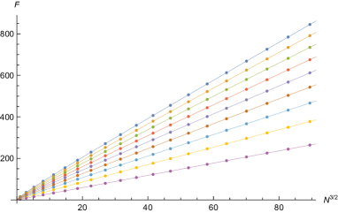
(a) free energy of $O(2N)+A$ model	(b) free energy of $O(2N+1)+A$ model

Figure 1: We show the plot of free energy $F=-\log Z(N,N_{f})$ of (a) $O(2N)+A$ model and (b) $O(2N+1)+A$ model for $N_{f}=1,2,\cdots,9$. Note that the horizontal axis is $N^{3/2}$. In both figures (a) and (b), $N_{f}$ increases from the bottom curve $(N_{f}=1)$ to the top curve $(N_{f}=9)$. The dots in the figures are the exact values of free energy at integer $N$, while the solid curves represent the perturbative free energy $F_{\text{pert}}=-\log Z_{\text{pert}}(N,N_{f})$ given by the Airy function (17) with $C,B$ and $A$ in Table 2.

In Figure 1, we show the plot of free energy for the $O(n)+A$ models. As we can see, the exact values of free energy at integer $N$ exhibit a nice agreement with the perturbative free energy (17) if we use the coefficients $C,B$ and $A$ in Table 2. We also find a similar agreement for the $O(n)+S$ models.

Let us explain in more detail how we found the results in Table 2. The coefficient $B$ can be found easily by matching the Airy function (17) with the exact values of $Z(N,N_{f})$, since the $N_{f}$-dependence of $B$ is relatively simple. On the other hand, the constant $A$ is a complicated function of $N_{f}$. To find the constant $A$ as a function of $N_{f}$, first we estimated the numerical values of $A$ by

$$A\approx\log\left[\frac{Z(N,N_{f})}{C^{-\frac{1}{3}}\text{Ai}\Bigl{[}C^{-\frac{1}{3}}(N-B)\Bigr{]}}\right],\quad(N\gg 1),$$ (22)

for $N$ as large as possible. In practice, we set $N=N_{\text{max}}$ in (22) where $N_{\text{max}}$ is the maximal value of $N$ that the exact values of $Z(N,N_{f})$ is available. In this way, we obtained the constant $A$ for various values of $N_{f}$’s. Then, assuming that $A$ is written as a linear combination of $A_{c}(k)$ with some $k$’s, we fixed the coefficients of this linear combination, and finally we arrived at the expressions of $A$ in Table 2. In Figure 2, we show the plot of constant $A$ for the $O(2N+1)+A$ model as an example. We can clearly see a nice agreement between the numerical values of $A$ at integer $N_{f}$ estimated by using (22) and our proposal of $A$ in Table 2. We also find a similar agreement for the other models in Table 2.

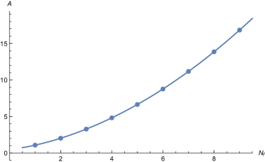
Figure 2: We show the plot of constant $A$ as a function of $N_{f}$ for the $O(2N+1)+A$ model. The dots are the numerical values of $A$ estimated by using (22) for $N_{f}=1,2,\cdots,9$, while the solid curve is the plot of $A$ in Table 2.

In section 5, we will derive the coefficients $B$ and $A$ of the $O(2N+1)+A$ model from the WKB expansion. For other models, we could not find a systematic method to compute $B$ and $A$.

From Table 2, we find the following interesting relations between the $O(2N)$ models and the $O(2N+1)$ models

$$B^{O(2N)+A}-B^{O(2N+1)+A} =\frac{1}{2},$$ (23)

$$B^{O(2N)+S}-B^{O(2N+1)+S} =\frac{1}{2},$$

$$A^{O(2N)+A}-A^{O(2N+1)+A} =-(N_{f}+1)\log 2,$$

$$A^{O(2N)+S}-A^{O(2N+1)+S} =-(N_{f}+2)\log 2.$$

In section 6, we will argue that the right hand side of these relations can be naturally interpreted as the contributions of orientifold plane.

4 Non-perturbative corrections

In this section, we study the non-perturbative part $J_{\text{np}}(\mu)$ of grand potential. To find the coefficients in $J_{\text{np}}(\mu,N_{f})$ we follow the procedure in HMO2 . First we expand $e^{J_{\text{np}}(\mu)}$ as

$$e^{J_{\text{np}}(\mu)}=1+\sum_{w>0,n}g_{w,n}\mu^{n}e^{-w\mu},$$ (24)

where $g_{w,n}$ are some $\mu$-independent coefficients. Then the non-perturbative part $Z_{\text{np}}(N,N_{f})$ of partition function is written as a sum of Airy functions and their derivatives

$$Z_{\text{np}}(N,N_{f}) =Z(N,N_{f})-Z_{\text{pert}}(N,N_{f})=\int_{\mathcal{C}}\frac{d\mu}{2\pi i}e^{J_{\text{pert}}(\mu)-N\mu}(e^{J_{\text{np}}(\mu)}-1)$$ (25)

$$=C^{-\frac{1}{3}}e^{A}\sum_{w>0,n}g_{w,n}(-\partial_{N})^{n}\text{Ai}\Bigl{[}C^{-\frac{1}{3}}(N+w-B)\Bigr{]}.$$

By matching the exact values of $Z(N,N_{f})$ with the above expansion of $Z_{\text{np}}(N,N_{f})$, we can fix the coefficients of $J_{\text{np}}(\mu)$ order by order in the weight $w$ of instantons. Using this method, we find the non-perturbative corrections for various $N_{f}$’s, which are summarized in Appendix A.

4.1 $O(n)+A$

Let us first consider the model $O(n)+A$ where $n=2N$ or $n=2N+1$. From the result in Appendix A.1 and A.2, we conjecture that there are three types of instantons

$$\mathcal{O}(e^{-\frac{2\mu}{N_{f}}}),\quad\mathcal{O}(e^{-2\mu}),\quad\mathcal{O}(e^{-\mu}).$$ (26)

The first two types have natural analogues in the $N_{f}$ matrix model GM ; Hatsuda:2014vsa . On the other hand, the last one in (26) has no counterpart in the $N_{f}$ matrix model, hence it is natural to interpret it as the effect of orientifold plane. Following GM ; Hatsuda:2014vsa , let us call the first two types in (26) worldsheet instantons and membrane instantons, respectively. For the last type in (26), we will call them “half instantons”. Note that the weight of worldsheet instanton in the $N_{f}$ matrix model is $e^{-4\mu/N_{f}}$, which is related to the worldsheet instanton in our case (26) by a rescaling $N_{f}\to 2N_{f}$.

Worldsheet instanton

We conjecture that the worldsheet instanton corrections are given by

$$J_{\text{WS}}(\mu,N_{f}) =-\frac{N_{f}+2}{2\pi\sin\frac{\pi}{N_{f}}}\left(\frac{2\mu}{N_{f}}+1\right)e^{-\frac{2\mu}{N_{f}}}$$ (27)

$$+ \left[-\frac{(N_{f}+2)^{2}}{2\pi^{2}}\left(\frac{2\mu}{N_{f}}+1\right)^{2}+\frac{4(N_{f}+2)^{2}-N_{f}^{2}}{8\pi N_{f}}\frac{\sin\frac{3\pi}{N_{f}}}{\sin\frac{\pi}{N_{f}}\sin\frac{2\pi}{N_{f}}}\left(\frac{4\mu}{N_{f}}+1\right)\right.$$

$$\left.\qquad-\frac{(N_{f}+2)^{2}}{2N_{f}^{2}}\frac{\sin\frac{6\pi}{N_{f}}}{\sin\frac{\pi}{N_{f}}\sin\frac{2\pi}{N_{f}}\sin\frac{3\pi}{N_{f}}}\right]e^{-\frac{4\mu}{N_{f}}}+\mathcal{O}(e^{-\frac{6\mu}{N_{f}}}),$$

for both $O(2N)+A$ and $O(2N+1)+A$ models. For instance, for $N_{f}=6$ one can see that (27) correctly reproduces the result of $J_{\text{np}}(\mu,6)$ in (103) and (105). Note that (27) is very similar to the worldsheet instantons in the $N_{f}$ matrix model Hatsuda:2014vsa and those in the $(1,q)$-model at $k=2$ Hatsuda:2015lpa .

We can check this conjecture (27) in the same way as in Hatsuda:2014vsa . We first notice that for $N_{f}>4$ the worldsheet 2-instanton factor $e^{-4\mu/N_{f}}$ is larger than the factor $e^{-\mu}$ of half instanton in (26). Thus, the non-perturbative part of canonical partition function has the following expansion

$$Z_{\text{np}}=Z_{\text{WS}}^{(1)}+Z_{\text{WS}}^{(2)}+(\text{subleading~{}corrections}),\quad(N_{f}>4),$$ (28)

where $Z_{\text{WS}}^{(1)}$ and $Z_{\text{WS}}^{(2)}$ are the contributions of worldsheet 1-instanton and worldsheet 2-instanton to the canonical partition function. Now let us consider the following quantity

$$\delta=\frac{Z-Z_{\text{pert}}-Z_{\text{WS}}^{(1)}-Z_{\text{WS}}^{(2)}}{Z_{\text{pert}}}e^{\frac{4\mu_{*}}{N_{f}}},$$ (29)

where $\mu_{*}$ is given by (16). If our conjecture of worldsheet instantons (27) is correct, $\delta$ should be exponentially small in the large $N$ limit. In Figure 3, we plot the quantity $\delta$ for $N_{f}=5,7,8,9$ in the $O(2N+1)+A$ model. As we can see in Figure 3, $\delta$ indeed decays exponentially as $N$ becomes large. We have also checked this behavior for the $O(2N)+A$ model. We should also mention that we have performed a similar checks for other types of instantons studied below.

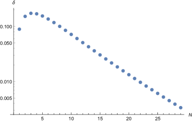
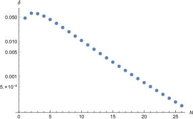
$N_{f}=5$	$N_{f}=7$
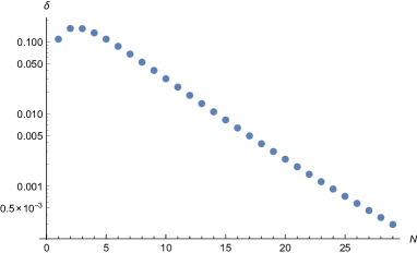
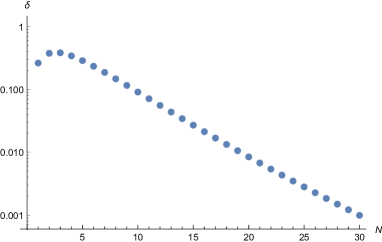
$N_{f}=8$	$N_{f}=9$

Figure 3: We show the plot of quantity $\delta$ in (29) for $N_{f}=5,7,8,9$ in the $O(2N+1)+A$ model. Note that the vertical axis is log scale.

Half instanton

From the results in Appendix A.1 and A.2, we conjecture that the half instantons are given by

$$J_{\text{half}}(\mu,N_{f}) =\varepsilon\frac{(\mu+1)}{\pi}2^{N_{f}}e^{-\mu}+\left[-\frac{(\mu+1)^{2}}{\pi^{2}}+\frac{N_{f}}{4}\right]2^{2N_{f}}e^{-2\mu}$$ (30)

$$\quad+\varepsilon\left[\frac{4(\mu+1)^{2}}{3\pi^{3}}-\frac{N_{f}(\mu+1)}{\pi}\right]2^{3N_{f}}e^{-3\mu}+\mathcal{O}(e^{-4\mu}),$$

where $\varepsilon$ is a sign depending on the parity of $n$ of the gauge group $O(n)$

$$\varepsilon=(-1)^{n}.$$ (31)

Let us take a closer look at these corrections. For instance, for the $N_{f}=2$ case, the order $\mathcal{O}(e^{-\mu})$ term comes from the 1-worldsheet instanton $J_{\text{WS}}^{(1)}$ and the 1-half instanton $J_{\text{half}}^{(1)}$, and our conjecture of worldsheet instantons (27) and half instantons (30) correctly reproduce the results in (103) and (105)

$$J_{\text{WS}}^{(1)}(\mu,2)+J_{\text{half}}^{(1)}(\mu,2)=\frac{(4\varepsilon-2)(\mu+1)}{\pi}e^{-\mu}.$$ (32)

Also, for the $N_{f}=4$ case, the order $\mathcal{O}(e^{-\mu})$ term comes from the 2-worldsheet instanton $J_{\text{WS}}^{(2)}$ and the 1-half instanton $J_{\text{half}}^{(1)}$, and the sum of these two contributions correctly reproduces the results in (103) and (105)

$$J_{\text{WS}}^{(2)}(\mu,4)+J_{\text{half}}^{(1)}(\mu,4)=\left[-\frac{9(\mu+2)^{2}}{2\pi^{2}}+\frac{(4+16\varepsilon)(\mu+1)}{\pi}+\frac{9}{4}\right]e^{-\mu}.$$ (33)

We should stress that our conjecture of half instantons (30) is consistent with all results in Appendix A.1 and A.2 in a very non-trivial way.

Bound states

The results in Appendix A.1 and A.2 suggest that there are various types of bound state contributions. The existence of such bound state contributions are first observed in ABJM theory HMO2 ; HMO-bound . Let us denote the bound state of $\ell$-worldsheet instanton, $m$-membrane instantons, and $n$-half instantons as $J^{(\ell,m,n)}(\mu,N_{f})$. Namely,

$$J^{(\ell,m,n)}(\mu,N_{f})\propto e^{-\frac{2\ell\mu}{N_{f}}-2m\mu-n\mu}.$$ (34)

For instance, there seems to exist a bound state of 1-worldsheet instanton $e^{-2\mu/N_{f}}$ and 1-half instanton $e^{-\mu}$. From the coefficient of $\mathcal{O}(e^{-2\mu/N_{f}-\mu})$ term for $N_{f}=3,1/2,3/2,5/2$ in Appendix A.1 and A.2, we conjecture

$$J^{(1,0,1)}(\mu,N_{f})=\varepsilon\frac{2^{N_{f}+1}}{\sin\frac{\pi}{N_{f}}}e^{-\frac{2\mu}{N_{f}}-\mu}.$$ (35)

There should also exist a bound state $J^{(0,1,1)}$ of 1-membrane instanton $e^{-2\mu}$ and 1-half instanton $e^{-\mu}$ in order to reproduce the finite term of $N_{f}=1$ at order $\mathcal{O}(e^{-3\mu})$

$$\lim_{N_{f}\to 1}\Big{[}J^{(1,0,1)}(\mu,N_{f})+J^{(0,1,1)}(\mu,N_{f})+J^{(0,0,3)}(\mu,N_{f})\Big{]}=\varepsilon\frac{88\mu+52/3}{3\pi}e^{-3\mu}.$$ (36)

Note that $J^{(1,0,1)}$ in (35) has a pole at $N_{f}=1$, while the 3-half instanton $J^{(0,0,3)}$ in (30) is regular at $N_{f}=1$. For the equation (36) to make sense, the bound state of membrane instanton and half instanton $J^{(0,1,1)}$ should cancel the pole coming from $J^{(1,0,1)}$ in (35). This pole cancellation mechanism, first discovered in the ABJM theory HMO2 , gives a constraint for the possible form of the coefficient of $J^{(0,1,1)}$. But this condition alone is not strong enough to determine $J^{(0,1,1)}$.

Membrane instanton

We do not have a direct information of the coefficient of membrane instantons in the results of Appendix A.1 and A.2. However, from the pole cancellation mechanism and the information of finite terms at $N_{f}=1,2$, we can make a conjecture of membrane 1-instanton, as we will see below.

From the expression of the membrane instanton in the $N_{f}$ matrix model Hatsuda:2015lpa , it is natural to conjecture that the coefficient of 1-membrane instanton is proportional to $2\mu+1$

$$J_{\text{M2}}(\mu,N_{f}) =b_{1}(N_{f})(2\mu+1)e^{-2\mu}+\mathcal{O}(e^{-4\mu}).$$ (37)

From (104) and (106), we observe that the 1-membrane instanton term is absent for half-integer $N_{f}$. Thus, the coefficients $b_{1}(N_{f})$ should vanish at half-integer $N_{f}$

$$b_{1}(N_{f})=0,\quad\Bigl{(}N_{f}\in\mathbb{Z}_{\geq 0}+\frac{1}{2}\Bigr{)}.$$ (38)

Also, the result of $N_{f}$ matrix model in Hatsuda:2014vsa suggests that $b_{1}(N_{f})$ is given by a certain combination of gamma-functions. Furthermore, $J_{\text{M2}}^{(1)}$ should reproduce the finite terms at $N_{f}=1,2$ in (103) and (105)

$$\lim_{N_{f}\to 1}\Bigl{[}J_{\text{WS}}^{(1)}+J_{\text{half}}^{(2)}+J_{\text{M2}}^{(1)}\Bigr{]} =\left[-\frac{10\mu^{2}+7\mu+7/2}{\pi^{2}}+1\right]e^{-2\mu},$$ (39)

$$\lim_{N_{f}\to 2}\Bigl{[}J_{\text{WS}}^{(2)}+J_{\text{half}}^{(2)}+J_{\text{M2}}^{(1)}+J^{(1,0,1)}\Bigr{]} =\left[-\frac{39\mu^{2}+63\mu/2+63/4}{\pi^{2}}+14+8\varepsilon\right]e^{-2\mu}.$$

Since $J_{\text{WS}}^{(1)}$ and $J_{\text{WS}}^{(2)}$ have poles at $N_{f}=1$ and $N_{f}=2$, respectively, 1-membrane instanton $J_{\text{M2}}^{(1)}$ should cancel those poles and give the finite terms in the right hand side of (39). From this pole cancellation condition and other conditions mentioned above, we conjecture that $J_{\text{M2}}^{(1)}$ is given by

$$J_{\text{M2}}^{(1)}(\mu,N_{f})=\frac{\Gamma(-N_{f})^{2}}{8\pi^{2}\Gamma(-2N_{f}-1)}(2\mu+1)e^{-2\mu}.$$ (40)

One can show that our conjecture (40) indeed reproduces the right hand side of (39) and vanishes when $N_{f}$ is positive half-integer, as required. It would be nice to see if our conjecture (40) of 1-membrane instanton is correct or not, by computing it from the WKB expansion as in Hatsuda:2015lpa ; Hatsuda:2014vsa .

4.2 $O(n)+S$

Next consider the model $O(n)+S$ with $n=2N$ or $n=2N+1$. From the results in Appendix A.3 and A.4, there seems to be two types of instantons

$$\mathcal{O}(e^{-\frac{2\mu}{N_{f}}}),\quad\mathcal{O}(e^{-2\mu}),$$ (41)

which are the analogue of worldsheet instantons and membrane instantons in the $N_{f}$ matrix model. There are no $\mathcal{O}(e^{-\mu})$ term in this case.

We conjecture that the worldsheet instanton corrections are given by

$$J_{\text{WS}}(\mu,N_{f})= -\frac{N_{f}}{2\pi\sin\frac{\pi}{N_{f}+2}}\left(\frac{2\mu}{N_{f}+2}+1\right)e^{-\frac{2\mu}{N_{f}+2}}$$ (42)

$$+\left[-\frac{N_{f}^{2}}{2\pi^{2}}\left(\frac{2\mu}{N_{f}+2}+1\right)^{2}+\frac{4N_{f}^{2}-(N_{f}+2)^{2}}{8\pi(N_{f}+2)}\frac{\sin\frac{3\pi}{N_{f}+2}}{\sin\frac{\pi}{N_{f}+2}\sin\frac{2\pi}{N_{f}+2}}\left(\frac{4\mu}{N_{f}+2}+1\right)\right.$$

$$\left.\qquad-\frac{N_{f}^{2}}{2(N_{f}+2)^{2}}\frac{\sin\frac{6\pi}{N_{f}+2}}{\sin\frac{\pi}{N_{f}+2}\sin\frac{2\pi}{N_{f}+2}\sin\frac{3\pi}{N_{f}+2}}\right]e^{-\frac{4\mu}{N_{f}+2}}+\mathcal{O}(e^{-\frac{6\mu}{N_{f}+2}}).$$

We have performed a similar check as in Figure 3 for our conjecture (42), and confirmed that (42) correctly reproduce the large $N$ behavior of exact values $Z(N,N_{f})$ for various $N_{f}$’s.

As for the membrane instantons, we were unable to determine their coefficient from the data in Appendix A.3 and A.4 alone. It would be interesting to study the structure of instanton corrections in this model further.

5 WKB expansion (I)

As discussed in Assel:2015hsa , we can compute the coefficients $C$ and $B$ in the perturbative part of grand potential by formally introducing the Planck constant $\hbar$ and performing the small $\hbar$ expansion, although the physical theory corresponds to $\hbar=2\pi$. Since the coefficients $C$ and $B$ receive corrections only up to order $\mathcal{O}(\hbar^{0})$ and $\mathcal{O}(\hbar^{2})$, respectively, we can fix $C$ and $B$ by computing the first two terms of WKB expansion and simply setting $\hbar=2\pi$ at the end. On the other hand, the coefficient $A$ receives all order corrections in $\hbar$, hence it is not obvious if we can find the constant $A$ in $J_{\text{pert}}(\mu)$ from this formal WKB expansion. Nevertheless, as we will see below, at least for the $O(2N+1)+A$ model we can guess the all order expression of the WKB expansion of $A$, and by setting $\hbar=2\pi$ we find the constant $A$ in a closed form. For models other than $O(2N+1)+A$, we found difficulty in computing the leading (classical) term in the WKB expansion. Therefore, in this section we will focus on the $O(2N+1)+A$ model. Note that, the $O(2N+1)+A$ model is related to the $USp(2N)+A$ model by a shift of $N_{f}$ (7), which in turn is dual to a $\widehat{D}$-type quiver theory by mirror symmetry deBoer:1996mp .

5.1 WKB expansion in $O(2N+1)+A$ model

As discussed in Assel:2015hsa , the density matrix $\rho(x,y)$ in (2) for the $O(2N+1)+A$ model can be written as a matrix element $\langle x|\rho|y\rangle$ of the quantum mechanical operator $\rho=e^{-H}$ of the following form

$$\rho =\rho_{D}\frac{1+R}{2},$$

$$\rho_{D} =\frac{2\sinh\frac{\widehat{x}}{2}}{(2\cosh\frac{\widehat{x}}{2})^{2N_{f}+3}}\left(\sinh\frac{\widehat{x}}{2}\frac{1}{\cosh\frac{\widehat{p}}{2}}\cosh\frac{\widehat{x}}{2}+\cosh\frac{\widehat{x}}{2}\frac{1}{\cosh\frac{\widehat{p}}{2}}\sinh\frac{\widehat{x}}{2}\right),$$

where $\widehat{x}$ and $\widehat{p}$ are the canonical variables obeying

$$[\widehat{x},\widehat{p}]=i\hbar,\qquad\hbar=2\pi,$$ (44)

and $R$ in (5.1) is the reflection operator flipping the sign of $x$

$$R|x\rangle=|-x\rangle.$$ (45)

Note that in Mezei:2013gqa a different expression of operator $\rho$ was used. We will consider the operator in Mezei:2013gqa in the next section. One advantage of $\rho_{D}$ in (5.1) is that it has not only a reflection symmetry $[\rho_{D},R]=0$, but also has a property that its trace with $R$ insertion vanishes Assel:2015hsa

$$\operatorname{Tr}(\rho_{D}^{\ell}R)=0,\qquad(\ell=1,2,\cdots).$$ (46)

This implies that the grand partition function is written as

$$\Xi(\mu)=\text{Det}(1+e^{\mu}\rho)=\sqrt{\text{Det}(1+e^{\mu}\rho_{D})},$$ (47)

and the grand potential is given by

$$J(\mu)=\frac{1}{2}\sum_{\ell=1}^{\infty}\frac{(-1)^{\ell-1}e^{\ell\mu}}{\ell}\operatorname{Tr}\rho_{D}^{\ell}.$$ (48)

As noticed in Hatsuda:2015oaa , the WKB expansion of the grand potential (48) is most easily obtained from the WKB expansion of the spectral trace $\operatorname{Tr}\rho_{D}^{s}$. By analytically continuing $\operatorname{Tr}\rho_{D}^{s}$ from integer $s$ to arbitrary complex $s$, the grand potential is written as a Mellin-Barnes type integral

$$J(\mu)=-\frac{1}{2}\int_{\gamma}\frac{ds}{2\pi i}\Gamma(-s)\Gamma(s)e^{s\mu}\operatorname{Tr}\rho_{D}^{s},$$ (49)

where the integration contour $\gamma$ is parallel to the imaginary axis with $0<\Re(s)<1$. By picking up poles at positive integers $s=\ell\in\mathbb{Z}_{>0}$, we recover (48). On the other hand, deforming the contour in the direction $\Re(s)\leq 0$, we can find a large $\mu$ expansion of $J(\mu)$. The WKB expansion of spectral trace takes the following form

$$\operatorname{Tr}\rho_{D}^{s} =Z_{0}(s)D(s,\hbar),$$ (50)

$$D(s,\hbar) =1+\sum_{n=1}^{\infty}D_{n}(s)\hbar^{2n}.$$

The leading term $Z_{0}(s)$ is given by the classical phase space integral, simply replacing the operators $(\widehat{x},\widehat{p})$ in (5.1) by classical commuting variables $(X,P)$

$$Z_{0}(s)=\int\frac{dXdP}{2\pi\hbar}\left[\frac{(2\sinh\frac{X}{2})^{2}}{2\cosh\frac{P}{2}(2\cosh\frac{X}{2})^{2N_{f}+2}}\right]^{s}=\frac{1}{2\pi\hbar}\frac{2\Gamma(s/2)^{2}\Gamma(2s)\Gamma(N_{f}s)\Gamma((N_{f}+1)s)}{\Gamma(s)^{2}\Gamma(2(N_{f}+1)s)}.$$ (51)

From the WKB expansion of the spectral trace (50), we can easily find the WKB expansion of grand potential by replacing $s$ in $D(s,\hbar)$ by the $\mu$-derivative $\partial_{\mu}$, and acting it on the leading term

$$J(\mu)=D(\partial_{\mu},\hbar)J_{0}(\mu),$$ (52)

where $J_{0}(\mu)$ is the leading term in the WKB expansion of grand potential

$$J_{0}(\mu)=-\frac{1}{2}\int_{\gamma}\frac{ds}{2\pi i}\Gamma(-s)\Gamma(s)e^{s\mu}Z_{0}(s).$$ (53)

Now, let us move on to the computation of $D_{n}(s)$ in (50). In many examples of $d=3~{}\mathcal{N}=4$ theories Moriyama:2014waa ; Hatsuda:2015lpa , it turned out that $D_{n}(s)$ was a rational function of $s$. Therefore, it is natural to assume that this is also the case for our expansion (50). Then, the easiest way to determine $D_{n}(s)$ is to make an ansatz that $D_{n}(s)$ is a rational function of $s$, and fix the coefficients in the ansatz by matching the WKB expansion of $\operatorname{Tr}\rho_{D}^{\ell}$ for integer $\ell$ from $\ell=1$ to some $\ell=\ell_{\text{max}}$, where we choose $\ell_{\text{max}}$ as the number of independent coefficients in the ansatz of $D_{n}(s)$. Once we determined $D_{n}(s)$ in this way, we can check the agreement of $\operatorname{Tr}\rho_{D}^{\ell}$ and $D_{n}(\ell)$ for $\ell>\ell_{\text{max}}$.

To compute the WKB expansion of $\operatorname{Tr}\rho_{D}^{\ell}$ for integer $\ell$, it is convenient to use the Wigner transform of the operator $\rho_{D}$. In general, the Wigner transform $O_{W}$ is defined by

$$O_{W}=\int dye^{\frac{iPy}{\hbar}}\Big{\langle}X-\frac{1}{2}y\Big{|}O\Big{|}X+\frac{1}{2}y\Big{\rangle}.$$ (54)

As explained in Appendix B, the Wigner transform of $\rho_{D}$ is given by

$$(\rho_{D})_{W}=\frac{2\sinh\frac{X}{2}}{(2\cosh\frac{X}{2})^{2N_{f}+3}}\star\frac{\sinh X}{\cosh\frac{P}{2}}.$$ (55)

Using the property of Wigner transformation

$$(AB)_{W}=A_{W}\star B_{W}\equiv A_{W}e^{\frac{i\hbar}{2}(\overleftarrow{\partial_{X}}\overrightarrow{\partial_{P}}-\overleftarrow{\partial_{P}}\overrightarrow{\partial_{X}})}B_{W},$$ (56)

the Wigner transform of the $\ell^{\text{th}}$ power of $\rho_{D}$ is given by the star-product of $(\rho_{D})_{W}$’s

$$(\rho_{D}^{\ell})_{W}=\underbrace{(\rho_{D})_{W}\star\cdots\star(\rho_{D})_{W}}_{\ell}.$$ (57)

Now, let us consider the WKB expansion of $(\rho_{D}^{\ell})_{W}$

$$(\rho_{D}^{\ell})_{W}=\sum_{m=0}^{\infty}\rho^{\ell}_{(m)}\hbar^{m}.$$ (58)

From the obvious relation $(\rho_{D}^{\ell})_{W}=(\rho_{D})_{W}\star(\rho_{D}^{\ell-1})_{W}$, the coefficient $\rho^{\ell}_{(m)}$ of this expansion can be computed recursively in $\ell$

$$\rho^{\ell}_{(m)} =\sum_{n_{1}+n_{2}+n_{3}=m}\rho_{(n_{1})}\frac{(i/2)^{n_{2}}}{n_{2}!}\Big{(}\overleftarrow{\partial_{X}}\overrightarrow{\partial_{P}}-\overleftarrow{\partial_{P}}\overrightarrow{\partial_{X}}\Big{)}^{n_{2}}\rho^{\ell-1}_{(n_{3})}.$$ (59)

Using the fact that the trace $\operatorname{Tr}\rho_{D}^{\ell}$ is written as a classical phase space integral of $(\rho_{D}^{\ell})_{W}$

$$\operatorname{Tr}\rho_{D}^{\ell}=\int\frac{dXdP}{2\pi\hbar}(\rho_{D}^{\ell})_{W},$$ (60)

and plugging the WKB expansion of $(\rho_{D}^{\ell})_{W}$ (58) into (60), finally we find the WKB expansion of the trace $\operatorname{Tr}\rho_{D}^{\ell}$.

Using the above method, we have computed $D_{n}(s)$ up to $n=13$. We find that $D_{n}(s)$ has the following form

$$D_{n}(s)=\frac{p_{n}(s)}{96^{n}\prod_{j=1}^{n}(2(N_{f}+1)s+2j-1)(s+2j-1)},$$ (61)

where $p_{n}(s)$ is a $(4n)^{\text{th}}$ order polynomial of $s$. The first few terms are given by

$$p_{1}(s) =N_{f}s^{2}(1-s)(3+N_{f}+2(N_{f}+1)s),$$

$$p_{2}(s) =\frac{N_{f}s^{3}(1-s)}{10}\left[-28N_{f}(N_{f}+1)^{2}s^{4}-4(N_{f}+1)\left(25N_{f}^{2}+47N_{f}+2\right)s^{3}\right.$$

$$\quad+\left(-29N_{f}^{3}-438N_{f}^{2}-549N_{f}-56\right)s^{2}+\left(-41N_{f}^{3}-178N_{f}^{2}-603N_{f}-250\right)s$$

$$\qquad\left.-6\left(4N_{f}^{3}+2N_{f}^{2}+7N_{f}+67\right)\right],$$

$$p_{3}(s) =\frac{N_{f}s^{3}(1-s)}{105}\Bigl{[}372N_{f}^{2}(N_{f}+1)^{3}s^{8}+2N_{f}(N_{f}+1)^{2}\left(1829N_{f}^{2}+3059N_{f}+164\right)s^{7}$$

$$\quad+(N_{f}+1)\left(10807N_{f}^{4}+48062N_{f}^{3}+47327N_{f}^{2}+5356N_{f}+96\right)s^{6}$$

$$\quad+\frac{1}{2}\left(17423N_{f}^{5}+231087N_{f}^{4}+586289N_{f}^{3}+460893N_{f}^{2}+80084N_{f}+2976\right)s^{5}$$

$$\quad+\left(7477N_{f}^{5}+92925N_{f}^{4}+458458N_{f}^{3}+596733N_{f}^{2}+187615N_{f}+9432\right)s^{4}$$

$$\quad+\frac{1}{2}\left(12125N_{f}^{5}+96285N_{f}^{4}+570131N_{f}^{3}+1605111N_{f}^{2}+1117364N_{f}+97224\right)s^{3}$$

$$\quad+\left(8596N_{f}^{5}+38502N_{f}^{4}+39601N_{f}^{3}+376104N_{f}^{2}+838273N_{f}+188364\right)s^{2}$$

$$\quad+12\left(768N_{f}^{5}+1104N_{f}^{4}-812N_{f}^{3}+3112N_{f}^{2}+31519N_{f}+29029\right)s$$

$$\quad+180\left(16N_{f}^{5}+2N_{f}^{2}+7N_{f}+1015\right)\Bigr{]}.$$

From this we can read off the general structure of $p_{n}(s)$ for $n\geq 2$

$$p_{n}(s)=N_{f}(1-s)s^{3}\sum_{j=0}^{4n-4}s^{j}g_{n}^{(j)}(N_{f}),$$ (62)

where $g_{n}^{(j)}(N_{f})$ is a $(2n-1)^{\text{th}}$ order polynomial of $N_{f}$. Note that $p_{1}(s)$ is an exception: $p_{1}(s)$ has a factor $s^{2}(1-s)$ while $p_{n}(s)~{}(n\geq 2)$ has a factor $s^{3}(1-s)$. As we will see in the next subsection, this is related to the difference of the $\hbar$ corrections of $C,B$ and $A$.

5.2 Perturbative part of $O(2N+1)+A$ from WKB expansion

By deforming the contour $\gamma$ to the left half plane $\Re(s)\leq 0$ in (49), we can find the large $\mu$ expansion of the grand potential $J(\mu)$. It turns out that the perturbative part $J_{\text{pert}}(\mu)$ comes from the pole at $s=0$. The leading contribution of the WKB expansion reads

$$J_{\text{pert},(0)}(\mu)=-\frac{1}{2}\oint_{s=0}\frac{ds}{2\pi i}\Gamma(-s)\Gamma(s)e^{s\mu}Z_{0}(s)$$ (63)

$$=\frac{\mu^{3}}{6N_{f}\pi^{2}}+\left(\frac{1}{8N_{f}}-\frac{N_{f}+3}{6}\right)\mu+\frac{\zeta(3)}{4N_{f}\pi^{2}}+\frac{(2N_{f}^{2}+7N_{f}+7N_{f})\zeta(3)}{\pi^{2}}.$$

The $\hbar$-corrections can be computed systematically by applying the relation (52) to the perturbative part

$$J_{\text{pert}}(\mu)=D(\partial_{\mu},\hbar)J_{\text{pert},(0)}(\mu).$$ (64)

Since $J_{\text{pert},(0)}(\mu)$ is a cubic polynomial in $\mu$, the derivatives $\partial_{\mu}^{m}$ with $m\geq 4$ do not contribute to $J_{\text{pert}}(\mu)$. By expanding $D_{n}(\partial_{\mu})$ up to $\partial_{\mu}^{3}$, we find

$$D_{n}(\partial_{\mu})=\delta_{n,1}\frac{N_{f}(N_{f}+3)}{96}\partial_{\mu}^{2}$$ (65)

$$+\frac{N_{f}}{4}\frac{(-1)^{n}B_{2n}B_{2n-2}}{(2n)!2^{2n}}\Bigl{[}(2N_{f})^{2n-1}+2(2N_{f}^{2}+7N_{f}+7)+2\cdot 4^{2n-1}-2^{2n-1}\Bigr{]}\partial_{\mu}^{3}+\mathcal{O}(\partial_{\mu}^{4}).$$

We have checked this behavior up to $n=13$ and we believe that this is true for all $n$.

From the expansion in (65), one can easily see that $C$ and $B$ receive corrections only up to $\mathcal{O}(\hbar^{0})$ and $\mathcal{O}(\hbar^{2})$, respectively. Acting the differential operator on the leading term $J_{\text{pert},(0)}$ and setting $\hbar=2\pi$, finally we arrive at the correct $C$ and $B$ of the $O(2N+1)+A$ model in Table 2

$$\left(1+\frac{N_{f}(N_{f}+3)}{96}\partial_{\mu}^{2}\hbar^{2}\right)J_{\text{pert},(0)}\Big{|}_{\hbar=2\pi}=\frac{\mu^{3}}{6N_{f}\pi^{2}}+\left(\frac{1}{8N_{f}}-\frac{N_{f}+3}{8}\right)\mu+\mathcal{O}(\mu^{0}).$$ (66)

We can also determine the constant $A$ by summing over all order corrections. From (63) and (65), one can easily see that the constant $A$ is given by

$$A =\frac{\zeta(3)}{4N_{f}\pi^{2}}+\frac{(2N_{f}^{2}+7N_{f}+7N_{f})\zeta(3)}{\pi^{2}}$$ (67)

$$+\sum_{n=1}^{\infty}\frac{N_{f}}{4}\frac{(-1)^{n}B_{2n}B_{2n-2}}{(2n)!2^{2n}}\Bigl{[}(2N_{f})^{2n-1}+2(2N_{f}^{2}+7N_{f}+7)+2\cdot 4^{2n-1}-2^{2n-1}\Bigr{]}\partial_{\mu}^{3}\hbar^{2n}\frac{\mu^{3}}{6N_{f}\pi^{2}}\Big{|}_{\hbar=2\pi}$$

$$=\frac{\zeta(3)}{4N_{f}\pi^{2}}+\frac{(2N_{f}^{2}+7N_{f}+7N_{f})\zeta(3)}{\pi^{2}}$$

$$+\frac{1}{4}\sum_{n=1}^{\infty}\frac{(-1)^{n}B_{2n}B_{2n-2}\pi^{2n-2}}{(2n)!}\Bigl{[}(2N_{f})^{2n-1}+2(2N_{f}^{2}+7N_{f}+7)+2\cdot 4^{2n-1}-2^{2n-1}\Bigr{]}.$$

By comparing this with the small $k$ expansion of $A_{c}(k)$ KEK

$$A_{c}(k)=\frac{2\zeta(3)}{\pi^{2}k}+\sum_{n=1}^{\infty}\frac{(-1)^{n}}{(2n)!}B_{2n}B_{2n-2}\pi^{2n-2}k^{2n-1},$$ (68)

we find that $A$ is written as

$$A=\frac{1}{4}A_{c}(2N_{f})+\frac{2N_{f}^{2}+7N_{f}+7}{2}A_{c}(1)+\frac{2A_{c}(4)-A_{c}(2)}{4}.$$ (69)

Using the explicit values of $A_{c}(4)$ and $A_{c}(2)$ from (19)

$$A_{c}(4)=-\frac{\zeta(3)}{4\pi^{2}}-\frac{1}{2}\log 2,\quad A_{c}(2)=-\frac{\zeta(3)}{2\pi^{2}},$$ (70)

one can see that (69) correctly reproduces the constant $A$ of the $O(2N+1)+A$ model in Table 2.

5.3 Comment on the non-perturbative part of $O(2N+1)+A$

In principle, we can also study the non-perturbative corrections $J_{\text{np}}(\mu)$ from the WKB analysis in the previous subsection. $J_{\text{np}}(\mu)$ comes from the poles on the negative real axis in the Mellin-Barnes representation (49). For instance, the leading term of spectral trace $Z_{0}(s)$ has poles at $s=-1/2$ and $s=-1/N_{f}$, and their contribution to $J_{\text{np}}(\mu)$ is given by

$$J_{\text{np}}(\mu)=\frac{1}{\hbar}D(\partial_{\mu},\hbar)\left[-\frac{2^{4+N_{f}}\pi^{\frac{3}{2}}}{\Gamma(\frac{1}{4})^{2}}e^{-\frac{\mu}{2}}-\frac{4(N_{f}+2)\pi\Gamma(\frac{1}{N_{f}})}{\sin^{2}\frac{\pi}{2N_{f}}\Gamma(\frac{1}{2N_{f}})^{2}}e^{-\frac{\mu}{N_{f}}}+\cdots\right]$$ (71)

$$=\frac{1}{\hbar}\left[-\frac{2^{4+N_{f}}\pi^{\frac{3}{2}}}{\Gamma(\frac{1}{4})^{2}}D\Bigl{(}-\frac{1}{2},\hbar\Bigr{)}e^{-\frac{\mu}{2}}-\frac{4(N_{f}+2)\pi\Gamma(\frac{1}{N_{f}})}{\sin^{2}\frac{\pi}{2N_{f}}\Gamma(\frac{1}{2N_{f}})^{2}}D\Bigl{(}-\frac{1}{N_{f}},\hbar\Bigr{)}e^{-\frac{\mu}{N_{f}}}+\cdots\right].$$

For these two terms, we find an all order expression of the coefficients. For the $e^{-\mu/N_{f}}$ term, we find

$$D\Bigl{(}-\frac{1}{N_{f}},\hbar\Bigr{)}=\frac{\hbar}{4}\cot\Bigl{(}\frac{\hbar}{4}\Bigr{)}\exp\left[\sum_{n=1}^{\infty}\frac{(-1)^{n-1}B_{2n}}{2n(2n+1)!}\Biggl{(}2B_{2n+1}\Bigl{(}\frac{1}{2N_{f}}\Bigr{)}-B_{2n+1}\Bigl{(}\frac{1}{N_{f}}\Bigr{)}\Biggr{)}(N_{f}\hbar)^{2n}\right].$$ (72)

We have checked that this agrees with the WKB expansion up to $n=13$. For the $e^{-\mu/2}$ term, we observe that the coefficient $D(-1/2,\hbar)$ is independent of $N_{f}$,

$$D\Bigl{(}-\frac{1}{2},\hbar\Bigr{)}=1-\frac{\hbar^{2}}{64}-\frac{29\hbar^{4}}{122880}+\frac{53\hbar^{6}}{23592960}+\cdots,$$ (73)

hence it is simply given by setting $N_{f}=2$ in (72). From (72), one can see that the coefficients of $e^{-\mu/N_{f}}$ and $e^{-\mu/2}$ both vanish in the limit $\hbar\to 2\pi$. This is consistent with our result in Appendix A.2 that there are no $e^{-\mu/N_{f}}$ and $e^{-\mu/2}$ terms in the grand potential of $O(2N+1)+A$ model. Note that (72) is essentially equal to a combination of $q$-gamma functions $\Gamma_{q}(\frac{1}{N_{f}})/\Gamma_{q}(\frac{1}{2N_{f}})^{2}$ with $q=e^{iN_{f}\hbar}$. A similar expression of instanton coefficient has appeared in the $(1,q)$-model studied in Hatsuda:2015lpa .

It is more interesting to determine the coefficients of $e^{-\mu},e^{-2\mu},$ or $e^{-2\mu/N_{f}}$ terms, which have non-vanishing contributions at $\hbar=2\pi$. However, using our data of WKB expansion alone, we were unable to find an all order expression of those terms and set $\hbar=2\pi$. It would be interesting to find those coefficients by computing the WKB expansion to more higher orders, or by other means.

6 WKB expansion (II)

In the previous section, we have considered the WKB expansion using $\rho$ satisfying $\operatorname{Tr}(\rho^{\ell}R)=0$ Assel:2015hsa . Alternatively, as in Mezei:2013gqa we can use $\rho$ with $\operatorname{Tr}(\rho^{\ell}R)\not=0$. In this section, we will consider the WKB expansion using the operator in the latter case. Interestingly, as we will see below we find that the $O(2N)+A$(or $S$) model and $O(2N+1)+A$(or $S$) model can be thought of as a $R=1$ and $R=-1$ subspace, respectively, of some bigger model. Namely the $O(n)$ model corresponds to a projection to

$$R=\varepsilon,$$ (74)

depending on the parity $\varepsilon=(-1)^{n}$ of $n$ in (31).

Using the relations

$$\langle x|\frac{1+R}{2\cosh\frac{\widehat{p}}{2}}|y\rangle=\frac{1}{2\pi}\frac{4\cosh\frac{x}{2}\cosh\frac{y}{2}}{2\cosh x+2\cosh y},\qquad\langle x|\frac{1-R}{2\cosh\frac{\widehat{p}}{2}}|y\rangle=\frac{1}{2\pi}\frac{4\sinh\frac{x}{2}\sinh\frac{y}{2}}{2\cosh x+2\cosh y},$$ (75)

one can show that the density matrices in (2) correspond to the following quantum mechanical operators $\rho=e^{-H}$

$$\rho=\left\{\begin{aligned} \rho_{A}\frac{1+\varepsilon R}{2}&\qquad\text{for}~{}~{}O(n)+A,\\ \rho_{S}\frac{1+\varepsilon R}{2}&\qquad\text{for}~{}~{}O(n)+S,\end{aligned}\right.$$ (76)

where $\rho_{A}$ and $\rho_{S}$ are given by

$$\rho_{A}=\frac{1}{2\cosh\frac{\widehat{p}}{2}}\frac{2\cosh\widehat{x}}{(2\cosh\frac{\widehat{x}}{2})^{2N_{f}+2}},\qquad\rho_{S}=\frac{1}{2\cosh\frac{\widehat{p}}{2}}\frac{(2\cosh\widehat{x})^{-1}}{(2\cosh\frac{\widehat{x}}{2})^{2N_{f}+2}},$$ (77)

with $[\widehat{x},\widehat{p}]=2\pi i$. Note that $\rho_{A}$ and $\rho_{S}$ have a reflection symmetry

$$[\rho_{A},R]=[\rho_{S},R]=0,$$ (78)

but $\operatorname{Tr}(\rho_{A,S}R)\not=0$. It is interesting that the density matrix of $O(n)+A$ model and $O(n)+S$ model can be written in a very similar form. We can treat $\rho_{A}$ and $\rho_{S}$ uniformly by introducing a sign $\sigma$

$$\sigma=\left\{\begin{aligned} +1&\quad\text{for}~{}\rho_{A},\\ -1&\quad\text{for}~{}\rho_{S}.\end{aligned}\right.$$ (79)

In other words, this sign $\sigma$ distinguishes the symmetric and anti-symmetric hypermultiplets. Then (77) can be written as

$$\rho_{\sigma}=\frac{1}{2\cosh\frac{\widehat{p}}{2}}\frac{(2\cosh\widehat{x})^{\sigma}}{(2\cosh\frac{\widehat{x}}{2})^{2N_{f}+2}}.$$ (80)

One can easily show that the total grand potential for $\rho=\rho_{\sigma}\frac{1+\varepsilon R}{2}$ can be decomposed as

$$J(\mu)=\frac{J_{\rho_{\sigma}}(\mu)+\varepsilon J_{\rho_{\sigma}}^{R}(\mu)}{2},$$ (81)

where

$$J_{\rho_{\sigma}}(\mu)=\sum_{\ell=1}^{\infty}\frac{(-1)^{\ell-1}e^{\ell\mu}}{\ell}\operatorname{Tr}(\rho_{\sigma}^{\ell}),\qquad J_{\rho_{\sigma}}^{R}(\mu)=\sum_{\ell=1}^{\infty}\frac{(-1)^{\ell-1}e^{\ell\mu}}{\ell}\operatorname{Tr}(\rho_{\sigma}^{\ell}R).$$ (82)

Note that (81) implies the following relation

$$J^{O(2N)+A}(\mu)-J^{O(2N+1)+A}(\mu) =J_{\rho_{A}}^{R}(\mu),$$ (83)

$$J^{O(2N)+S}(\mu)-J^{O(2N+1)+S}(\mu) =J_{\rho_{S}}^{R}(\mu).$$

The perturbative part of this relation is closely related to the difference of $B$ and $A$ found in (23). From the brane configuration in section 2, it is tempting to identify $J_{\rho_{\sigma}}^{R}(\mu)$ as the contribution of a half D2-brane stuck on the orientifold plane. In the rest of this section, we will consider the WKB expansion of this contribution.

Notice that $\operatorname{Tr}(OR)$ for some operator $O$ can be obtained from the Wigner transform $O_{W}$ by simply setting $X=P=0$

$$\operatorname{Tr}(OR)=\frac{1}{2}O_{W}\Big{|}_{X=P=0},$$ (84)

which follows directly from the definition of $O_{W}$ in (54)

$$O_{W}\Big{|}_{X=P=0}=\int dy\,\Big{\langle}\!-\frac{1}{2}y\Big{|}O\Big{|}\frac{1}{2}y\Big{\rangle}=2\operatorname{Tr}(OR).$$ (85)

Thus the WKB expansion of $\operatorname{Tr}(\rho_{\sigma}^{\ell}R)$ can be easily found from the WKB expansion of $(\rho_{\sigma}^{\ell})_{W}$, which can be systematically computed by using the method in the previous section. The Wigner transform of $\rho_{\sigma}$ is easily found to be

$$(\rho_{\sigma})_{W}=\frac{1}{2\cosh\frac{P}{2}}\star\frac{(2\cosh X)^{\sigma}}{(2\cosh\frac{X}{2})^{2N_{f}+2}}.$$ (86)

As in the previous section, $J_{\rho_{\sigma}}^{R}(\mu)$ has a Mellin-Barnes representation

$$J_{\rho_{\sigma}}^{R}(\mu)=-\int_{\gamma}\frac{ds}{2\pi i}\Gamma(-s)\Gamma(s)\operatorname{Tr}(\rho_{\sigma}^{s}R).$$ (87)

We will call $\operatorname{Tr}(\rho_{\sigma}^{s}R)$ in (87) the twisted spectral trace. The WKB expansion of $J_{\rho_{\sigma}}^{R}(\mu)$ can be found from the WKB expansion of twisted spectral trace $\operatorname{Tr}(\rho_{\sigma}^{s}R)$

$$\operatorname{Tr}(\rho_{\sigma}^{s}R) =Z_{0}^{R}(s)D^{R}(s,\hbar),$$

$$D^{R}(s,\hbar) =1+\sum_{n=1}^{\infty}D_{n}^{R}(s)\hbar^{2n}.$$

The leading term $Z_{0}^{R}(s)$ in (6) can be easily obtained as

$$Z_{0}^{R}(s)=2^{-1-s(2N_{f}+3-\sigma)}.$$ (88)

Note that the leading term $Z_{0}^{R}(s)$ of twisted spectral trace $\operatorname{Tr}(\rho_{\sigma}^{s}R)$ in (88) is order $\mathcal{O}(\hbar^{0})$, while the leading term $Z_{0}(s)$ of spectral trace $\operatorname{Tr}(\rho_{D}^{s})$ in (51) is order $\mathcal{O}(\hbar^{-1})$. We have computed $D_{n}^{R}(s)$ in (6) up to $n=9$ for both $\rho_{A}$ and $\rho_{S}$. For $\rho_{A}$, the first three terms are given by

$$D_{1}^{R}(s) =\frac{1}{64}(1-N_{f})s^{2},$$ (89)

$$D_{2}^{R}(s) =s^{2}\left(\frac{5(N_{f}-1)^{2}s^{2}}{24576}+\frac{(N_{f}+1)(2N_{f}-5)s}{8192}+\frac{(N_{f}+1)(2N_{f}-5)}{12288}\right),$$

$$D_{3}^{R}(s) =s^{2}\left(-\frac{61(N_{f}-1)^{3}s^{4}}{23592960}-\frac{7(N_{f}-1)(N_{f}+1)(2N_{f}-5)s^{3}}{1572864}\right.$$

$$\hskip 34.1433pt-\frac{(N_{f}+1)(34N_{f}^{2}-107N_{f}-17)s^{2}}{2359296}-\frac{(N_{f}-4)(N_{f}+1)(2N_{f}+3)s}{196608}$$

$$\hskip 34.1433pt\left.-\frac{(N_{f}+1)(2N_{f}^{2}-3N_{f}-29)}{737280}\right),$$

while for $\rho_{S}$, the first three terms are given by

$$D_{1}^{R}(s) =-\frac{1}{64}(N_{f}+3)s^{2},$$ (90)

$$D_{2}^{R}(s) =s^{2}\left(\frac{5(N_{f}+3)^{2}s^{2}}{24576}+\frac{(2N_{f}^{2}+13N_{f}+27)s}{8192}+\frac{2N_{f}^{2}+13N_{f}+27}{12288}\right),$$

$$D_{3}^{R}(s) =s^{2}\left(-\frac{61(N_{f}+3)^{3}s^{4}}{23592960}-\frac{7(N_{f}+3)(2N_{f}^{2}+13N_{f}+27)s^{3}}{1572864}\right.$$

$$\hskip 34.1433pt+\frac{(-34N_{f}^{3}-335N_{f}^{2}-1272N_{f}-1899)s^{2}}{2359296}+\frac{(-2N_{f}^{3}-21N_{f}^{2}-91N_{f}-168)s}{196608}$$

$$\hskip 34.1433pt\left.-\frac{(N_{f}+5)(2N_{f}^{2}+13N_{f}+51)}{737280}\right).$$

As discussed in the previous section, deforming the contour in the direction $\Re(s)\leq 0$ in (87), we can find the large $\mu$ expansion of $J_{\rho_{\sigma}}^{R}(\mu)$. The perturbative part comes from the pole at $s=0$. Since the higher order terms $D_{n}^{R}(s)$ has a zero at $s=0$ of order $s^{2}$, they do not contribute to the residue at $s=0$. Thus, the residue at $s=0$ comes only from the leading term $Z_{0}(s)$

$$-\oint_{s=0}\frac{ds}{2\pi i}\Gamma(-s)\Gamma(s)Z_{0}^{R}(s)e^{s\mu}=\frac{\mu}{2}-\frac{2N_{f}+3-\sigma}{2}\log 2.$$ (91)

One can see that (91) precisely reproduces the difference of $B$ and $A$ in (23) between the $O(2N)$ and $O(2N+1)$ models.

6.1 Comments on the non-perturbative corrections

By matching the WKB expansion of twisted spectral trace $\operatorname{Tr}(\rho_{\sigma}^{s}R)$, we find the first two non-perturbative corrections, coming from the poles at $s=-1$ and $s=-2$, in a closed form in $\hbar$

$$-\int\frac{ds}{2\pi i}\Gamma(-s)\Gamma(s)\operatorname{Tr}(\rho_{\sigma}^{s}R)e^{s\mu}$$ (92)

$$= \frac{\mu}{2}-\frac{2N_{f}+3-\sigma}{2}\log 2+\frac{(2\cos\frac{\hbar}{8})^{2(N_{f}+1)}}{(2\cos\frac{\hbar}{4})^{\sigma}}e^{-\mu}-\frac{(4\cos\frac{\hbar}{4})^{2(N_{f}+1)}}{(4\cos\frac{\hbar}{2})^{\sigma}}e^{-2\mu}+\mathcal{O}(e^{-3\mu}).$$

It is tempting to identify these corrections as the “half instantons”. For $\rho_{S}~{}(\sigma=-1)$, the non-perturbative corrections in (92) vanish at $\hbar=2\pi$, which is consistent with the absence of $\mathcal{O}(e^{-\mu})$ term in $O(n)+S$ models.

On the other hand, for $\rho_{A}~{}(\sigma=+1)$ the 1-instanton term has a pole at $\hbar=2\pi$

$$\lim_{\hbar\to 2\pi}\frac{(2\cos\frac{\hbar}{8})^{2(N_{f}+1)}}{2\cos\frac{\hbar}{4}}e^{-\mu}=\left[-\frac{2^{N_{f}+2}}{\hbar-2\pi}+(N_{f}+1)2^{N_{f}}\right]e^{-\mu}.$$ (93)

This should be canceled by a term of order $\mathcal{O}(e^{-2\pi\mu/\hbar})$, which is non-perturbative in $\hbar$ and hence cannot be seen directly in the WKB expansion. As discussed in Hatsuda:2015oaa , the $\mathcal{O}(e^{-2\pi\mu/\hbar})$ term might arise from a pole of the twisted spectral trace $\operatorname{Tr}(\rho_{A}^{s}R)$ at $s=-2\pi/\hbar$. Our result of 1-instanton and 2-instanton in (92) suggests that $\operatorname{Tr}(\rho_{A}^{s}R)$ has a structure

$$\operatorname{Tr}(\rho_{A}^{s}R)=\frac{f(s,N_{s})}{\cos\frac{s\hbar}{4}},$$ (94)

which has a pole at $s=-2\pi/\hbar$. As in Hatsuda:2015oaa , using the Pade approximation, we have checked numerically that $\operatorname{Tr}(\rho_{A}^{s}R)$ has a pole very close to $s=-2\pi/\hbar$. For the special value of $N_{f}=-1$, which is not physical though, by matching the WKB expansion we find a closed form expression of the twisted spectral trace $\operatorname{Tr}(\rho_{A}^{s}R)$

$$\operatorname{Tr}(\rho_{A}^{s}R)\Big{|}_{N_{f}=-1}=\frac{1}{2\cos\frac{s\hbar}{4}},$$ (95)

which indeed has a pole at $s=-2\pi/\hbar$, as expected. Although we do not have an analytic proof that $\operatorname{Tr}(\rho_{A}^{s}R)$ has a pole at $s=-2\pi/\hbar$ for general $N_{f}$, we will assume that this is the case in the rest of this section.

We assume that $\operatorname{Tr}(\rho_{A}^{s}R)$ has a simple pole at $s=-2\pi/\hbar$ for general $N_{f}$

$$\lim_{s\to-\frac{2\pi}{\hbar}}\operatorname{Tr}(\rho_{A}^{s}R)=\frac{1}{\hbar}\frac{r(\frac{2\pi}{\hbar})}{s+\frac{2\pi}{\hbar}}.$$ (96)

Then the contribution of pole at $s=-2\pi/\hbar$ to $J_{\rho_{A}}^{R}$ is given by

$$-\oint_{s=-\frac{2\pi}{\hbar}}\frac{ds}{2\pi i}\Gamma(-s)\Gamma(s)\operatorname{Tr}(\rho_{A}^{s}R)e^{s\mu}=\frac{r(\frac{2\pi}{\hbar})}{2\sin\frac{2\pi^{2}}{\hbar}}e^{-\frac{2\pi\mu}{\hbar}}.$$ (97)

This contribution has a pole at $\hbar=2\pi$, and behaves in the limit $\hbar\to 2\pi$ as

$$\lim_{\hbar\to 2\pi}\frac{r(\frac{2\pi}{\hbar})}{2\sin\frac{2\pi^{2}}{\hbar}}e^{-\frac{2\pi\mu}{\hbar}}=\left[\frac{r(1)}{\hbar-2\pi}+\frac{(\mu+1)r(1)-r^{\prime}(1)}{2\pi}\right]e^{-\mu}.$$ (98)

Thus, there is a possibility that the pole at $\hbar=2\pi$ cancels between (93) and (98). This pole cancellation occurs if $r(1)$ is given by

$$r(1)=2^{N_{f}+2}.$$ (99)

If we further assume

$$r^{\prime}(1)=\pi(N_{f}+1)2^{N_{f}+1},$$ (100)

then the total contribution correctly reproduces the 1-half instanton term in $J_{\text{half}}$ (30)

$$\frac{\varepsilon}{2}J_{\rho_{A}}^{R}=\varepsilon\frac{(\mu+1)}{\pi}2^{N_{f}}e^{-\mu}+\mathcal{O}(e^{-2\mu}).$$ (101)

For the $N_{f}=-1$ case in (95), one can see that the residue at $s=-2\pi/\hbar$ indeed satisfies the above conditions

$$r=2,\qquad r^{\prime}=0.$$ (102)

It would be interesting to study the analytic structure of $\operatorname{Tr}(\rho_{A}^{s}R)$ for general $N_{f}$ and see if it indeed has a pole at $s=-2\pi/\hbar$ with the correct residue.

7 Conclusion

In this paper, we have studied non-perturbative effects in $\mathcal{N}=4$ $O(n)$ Yang-Mills theories with $N_{f}$ fundamental and one (anti)symmetric hypermultiplets using the Fermi gas formalism for their $S^{3}$ partition functions. They are a natural generalization of $N_{f}$ matrix model and interesting in their own right since we can study the effects of orientifold plane in the strong coupling M-theoretic regime.

We determined the coefficients $C,B$ and $A$ in the perturbative part of grand potential as functions of $N_{f}$ in Table 2. We also studied instanton corrections to the grand potential using our exact values of canonical partition functions $Z(N,N_{f})$. We found that instanton corrections in the $O(n)+A$ model and the $O(n)+S$ model have slightly different structure. For the $O(n)+A$ model, in addition to the worldsheet instantons (27) and membrane instantons (40), there are “half instanton” corrections coming from the effect of orientifold plane. We have argued that half instantons can be naturally identified as the contributions from the twisted spectral trace $\operatorname{Tr}(\rho_{A}^{s}R)$ in the Fermi gas picture. Also, we found a bound state of worldsheet instanton and half instanton (35). From the pole cancellation argument, there should also be a bound state of membrane instanton and half instanton as well.

It is interesting that the reflection $R$ of one-dimensional Fermi gas system has a relation to the orientifolding in the spacetime. We find that the half instanton has a weight $e^{-\mu}$ which is half of the weight of membrane instanton $e^{-2\mu}$. This type of half instanton corrections is also observed in other theories Grassi:2014uua ; Moriyama:2015asx , and we believe that this is a general phenomenon in M-theory on orientifolds. It would be interesting to study the general structure of half instantons and clarify the precise relation to the Type IIA brane picture.

In the case of ABJM theory, the effect of bound state can be removed by introducing the effective chemical potential given by the quantum A-period HMO-bound ; HMMO . It would be very interesting to see whether a similar redefinition of chemical potential works in our case. To study instanton corrections further, it is desirable to find a systematic method to compute the WKB expansion. In the case of $N_{f}$ matrix model, it has a natural one-parameter generalization of the model by introducing a Chern-Simons level $k$, and we can systematically study the WKB expansion around $k=0$ Hatsuda:2015lpa . It would be interesting to find a generalization of the $O(n)+A$(or $S$) models with Chern-Simons terms, along the lines of Moriyama:2015jsa ; Assel:2015hsa .

Acknowledgments

I am grateful to Yasuyuki Hatsuda, Masazumi Honda, and Marcos Marino for useful discussions. I would also like to thank the theory group in University of Geneva for hospitality.

Appendix A $J_{\text{np}}(\mu,N_{f})$ for various $N_{f}$

In this Appendix, we summarize the non-perturbative corrections for various (half-)integral $N_{f}$, obtained from the data of exact values of $Z(N,N_{f})$.

A.1 $O(2N)+A$

Here we summarize the non-perturbative corrections $J_{\text{np}}(\mu,N_{f})$ to the grand potential of the $O(2N)+A$ model.

For integer $N_{f}$ we find

$$J_{\text{np}}(\mu,1) =\frac{2(\mu+1)}{\pi}e^{-\mu}+\left[-\frac{10\mu^{2}+7\mu+7/2}{\pi^{2}}+1\right]e^{-2\mu}+\frac{88\mu+52/3}{3\pi}e^{-3\mu}$$

$$J_{\text{np}}(\mu,2) =\frac{2(\mu+1)}{\pi}e^{-\mu}+\left[-\frac{39\mu^{2}+63\mu/2+63/4}{\pi^{2}}+22\right]e^{-2\mu}+\frac{664\mu+484/3}{3\pi}e^{-3\mu}$$

$$J_{\text{np}}(\mu,3) =-\frac{5}{\sqrt{3}\pi}\left(\frac{2\mu}{3}+1\right)e^{-\frac{2\mu}{3}}+\frac{8(\mu+1)}{\pi}e^{-\mu}+\left[-\frac{50(\mu+3/2)^{2}}{9\pi^{2}}+\frac{100}{27}\right]e^{-\frac{4\mu}{3}}+\frac{32}{\sqrt{3}}e^{-\frac{5\mu}{3}}$$

$$J_{\text{np}}(\mu,4) =-\frac{6}{\sqrt{2}\pi}\left(\frac{\mu}{2}+1\right)e^{-\frac{\mu}{2}}+\left[-\frac{9(\mu+2)^{2}}{2\pi^{2}}+\frac{20(\mu+1)}{\pi}+\frac{9}{4}\right]e^{-\mu}$$

$$J_{\text{np}}(\mu,6) =-\frac{8}{\pi}\left(\frac{\mu}{3}+1\right)e^{-\frac{\mu}{3}}+\left[-\frac{32(\mu+3)^{2}}{9\pi^{2}}+\frac{110(\mu+3/2)}{9\sqrt{3}\pi}\right]e^{-\frac{2\mu}{3}}$$ (103)

and for half-integer $N_{f}$ we find

$$J_{\text{np}}(\mu,1/2) =\frac{\sqrt{2}(\mu+1)}{\pi}e^{-\mu}+\left[-\frac{2(\mu+1)^{2}}{\pi^{2}}+\frac{1}{4}\right]e^{-2\mu}+\left[\frac{8\sqrt{2}(\mu+1)^{3}}{\pi^{3}}-\frac{\sqrt{2}(\mu+1)}{\pi}\right]e^{-3\mu}$$

$$J_{\text{np}}(\mu,3/2) =\frac{2\sqrt{2}(\mu+1)}{\pi}e^{-\mu}-\frac{7}{2\sqrt{3}\pi}\left(\frac{4\mu}{3}+1\right)e^{-\frac{4\mu}{3}}+\left[-\frac{8(\mu+1)^{2}}{\pi^{2}}+3\right]e^{-2\mu}+\frac{8\sqrt{2}}{\sqrt{3}}e^{-\frac{7\mu}{3}}$$

$$+\left[-\frac{49}{8\pi^{2}}\left(\frac{4\mu}{3}+1\right)^{2}+\frac{196}{27}\right]e^{-\frac{8\mu}{3}}+2^{\frac{9}{2}}\left[\frac{4(\mu+1)^{3}}{3\pi^{3}}-\frac{3}{2}\frac{\mu+1}{\pi}\right]e^{-3\mu}-\frac{64(\mu+1)}{\sqrt{3}\pi}e^{-\frac{10\mu}{3}}$$

$$J_{\text{np}}(\mu,5/2) =J_{\text{WS}}^{(1)}(\mu,5/2)+\frac{4\sqrt{2}(\mu+1)}{\pi}e^{-\mu}+J_{\text{WS}}^{(2)}(\mu,5/2)+\frac{2^{\frac{5}{2}+1}}{\sin\frac{2\pi}{5}}e^{-\frac{9\mu}{5}}+\left[-\frac{32(\mu+1)^{2}}{\pi^{2}}+20\right]e^{-2\mu}$$ (104)

where $J^{(n)}_{\text{WS}}(\mu,N_{f})$ is the worldsheet $n$-instanton contribution given by (27).

A.2 $O(2N+1)+A$

Here we summarize the non-perturbative corrections $J_{\text{np}}(\mu,N_{f})$ to the grand potential of the $O(2N+1)+A$ model.

For integer $N_{f}$ we find

$$J_{\text{np}}(\mu,1) =-\frac{2(\mu+1)}{\pi}e^{-\mu}+\left[-\frac{10\mu^{2}+7\mu+7/2}{\pi^{2}}+1\right]e^{-2\mu}-\frac{88\mu+52/3}{3\pi}e^{-3\mu}$$

$$J_{\text{np}}(\mu,2) =-\frac{6(\mu+1)}{\pi}e^{-\mu}+\left[-\frac{39\mu^{2}+63/2\mu+63/4}{\pi^{2}}+6\right]e^{-2\mu}-\frac{664\mu+484/3}{\pi}e^{-3\mu}$$

$$J_{\text{np}}(\mu,3) =-\frac{5}{\sqrt{3}\pi}\left(\frac{2\mu}{3}+1\right)e^{-\frac{2\mu}{3}}-\frac{8(\mu+1)}{\pi}e^{-\mu}+\left[-\frac{50(\mu+3/2)^{2}}{9\pi^{2}}+\frac{100}{27}\right]e^{-\frac{4\mu}{3}}-\frac{32}{\sqrt{3}}e^{-\frac{5\mu}{3}}$$

$$J_{\text{np}}(\mu,4) =-\frac{6}{\sqrt{2}\pi}\left(\frac{\mu}{2}+1\right)e^{-\frac{\mu}{2}}+\left[-\frac{9(\mu+2)^{2}}{2\pi^{2}}-\frac{12(\mu+1)}{\pi}+\frac{9}{4}\right]e^{-\mu}$$

$$J_{\text{np}}(\mu,6) =-\frac{8}{\pi}\left(\frac{\mu}{3}+1\right)e^{-\frac{\mu}{3}}+\left[-\frac{32(\mu+3)^{2}}{9\pi^{2}}+\frac{110(\mu+3/2)}{9\sqrt{3}\pi}\right]e^{-\frac{2\mu}{3}}$$ (105)

and for half-integer $N_{f}$ we find

$$J_{\text{np}}(\mu,1/2) =-\frac{\sqrt{2}}{\pi}(\mu+1)e^{-\mu}+\left[-\frac{2(\mu+1)^{2}}{\pi^{2}}+\frac{1}{4}\right]e^{-2\mu}+\left[-\frac{8\sqrt{2}(\mu+1)^{3}}{3\pi^{3}}+\frac{\sqrt{2}(\mu+1)}{\pi}\right]e^{-3\mu}$$

$$J_{\text{np}}(\mu,3/2) =-\frac{2\sqrt{2}}{\pi}(\mu+1)e^{-\mu}-\frac{7}{2\sqrt{3}\pi}\left(\frac{4\mu}{3}+1\right)e^{-\frac{4\mu}{3}}+\left[-\frac{8(\mu+1)^{2}}{\pi^{2}}+3\right]e^{-2\mu}-\frac{8\sqrt{2}}{\sqrt{3}}e^{-\frac{7\mu}{3}}$$

$$+\left[-\frac{49}{8\pi^{2}}\left(\frac{4\mu}{3}+1\right)^{2}+\frac{196}{27}\right]e^{-\frac{8\mu}{3}}+2^{\frac{9}{2}}\left[-\frac{4(\mu+1)^{3}}{3\pi^{3}}+\frac{3(\mu+1)}{2\pi}\right]e^{-3\mu}-\frac{64(\mu+1)}{\sqrt{3}\pi}e^{-\frac{10\mu}{3}}$$

$$J_{\text{np}}(\mu,5/2) =J_{\text{WS}}^{(1)}(\mu,5/2)-\frac{4\sqrt{2}}{\pi}(\mu+1)e^{-\mu}+J_{\text{WS}}^{(2)}(\mu,5/2)-\frac{2^{\frac{5}{2}+1}}{\sin\frac{2\pi}{5}}e^{-\frac{9\mu}{5}}+\left[-\frac{2^{5}(\mu+1)^{2}}{\pi^{2}}+20\right]e^{-2\mu}$$ (106)

where $J^{(n)}_{\text{WS}}(\mu,N_{f})$ is the worldsheet $n$-instanton contribution given by (27).

A.3 $O(2N)+S$

Here we summarize the non-perturbative corrections $J_{\text{np}}(\mu,N_{f})$ to the grand potential of the $O(2N)+S$ model.

For integer $N_{f}$ we find

$$J_{\text{np}}(\mu,-1) =\left[\frac{4\mu^{2}+2\mu+1}{2\pi^{2}}+2\right]e^{-2\mu}+\left[-\frac{52\mu^{2}+\mu+9/4}{4\pi^{2}}-14\right]e^{-4\mu}$$

$$+\left[\frac{386\mu^{2}-152\mu/3+77/9}{3\pi^{2}}+\frac{416}{3}\right]e^{-6\mu}$$

$$J_{\text{np}}(\mu,0) =\frac{4\mu^{2}+2\mu+1}{4\pi^{2}}e^{-2\mu}+\left[-\frac{52\mu^{2}+\mu+9/4}{8\pi^{2}}+2\right]e^{-4\mu}$$

$$+\left[\frac{386\mu^{2}-152\mu/3+77/9}{6\pi^{2}}-32\right]e^{-6\mu}$$

$$J_{\text{np}}(\mu,1) =-\frac{1}{\sqrt{3}\pi}\left(\frac{2\mu}{3}+1\right)e^{-\frac{2\mu}{3}}+\left[-\frac{2(\mu+3/2)^{2}}{9\pi^{2}}+\frac{4}{27}\right]e^{-\frac{4\mu}{3}}$$

$$J_{\text{np}}(\mu,2) =-\frac{2}{\sqrt{2}\pi}\left(\frac{\mu}{2}+1\right)e^{-\frac{\mu}{2}}+\left[-\frac{(\mu+2)^{2}}{2\pi^{2}}+\frac{1}{4}\right]e^{-\mu}$$

$$J_{\text{np}}(\mu,3) =-\frac{3}{2\pi\sin\frac{\pi}{5}}\left(\frac{2\mu}{5}+1\right)e^{-\frac{2\mu}{5}}$$

$$+\left[-\frac{9}{2\pi^{2}}\left(\frac{2\mu}{5}+1\right)^{2}+\frac{11}{40\pi\sin\frac{\pi}{5}}\left(\frac{4\mu}{5}+1\right)+\frac{9}{50\sin^{2}\frac{2\pi}{5}}\right]e^{-\frac{4\mu}{5}}$$

$$J_{\text{np}}(\mu,4) =-\frac{4}{\pi}\left(\frac{\mu}{3}+1\right)e^{-\frac{\mu}{3}}+\left[-\frac{8(\mu+3)^{2}}{9\pi^{2}}+\frac{14(\mu+3/2)}{9\sqrt{3}\pi}\right]e^{-\frac{2\mu}{3}}$$ (107)

and for half-integer $N_{f}$ we find

$$J_{\text{np}}(\mu,-3/2) =\frac{3(2\mu+1)}{2\pi}e^{-2\mu}+\left[-\frac{10\mu^{2}+7\mu/2+7/8}{\pi^{2}}-\frac{1}{4}\right]e^{-4\mu}+\frac{44\mu+13/3}{\pi}e^{-6\mu}$$

$$J_{\text{np}}(\mu,-1/2) =\frac{1}{2\sqrt{3}\pi}\left(\frac{4\mu}{3}+1\right)e^{-\frac{4\mu}{3}}+J_{\text{WS}}^{(2)}(\mu,-1/2)$$

$$J_{\text{np}}(\mu,1/2) =J_{\text{WS}}^{(1)}(\mu,1/2)+J_{\text{WS}}^{(2)}(\mu,1/2)$$ (108)

where $J^{(n)}_{\text{WS}}(\mu,N_{f})$ denotes the worldsheet $n$-instanton term in (42).

Note that the negative $N_{f}$ cases in the above list are unphysical for the $O(2N)+S$ theory. Nonetheless, the integral defining the partition functions are well-defined for those values of negative $N_{f}$.

A.4 $O(2N+1)+S$

Here we summarize the non-perturbative corrections $J_{\text{np}}(\mu,N_{f})$ to the grand potential of the $O(2N+1)+S$ model.

For integer $N_{f}$ we find

$$J_{\text{np}}(\mu,-1) =\left[\frac{4\mu^{2}+2\mu+1}{2\pi^{2}}-2\right]e^{-2\mu}+\left[-\frac{52\mu^{2}+\mu+9/4}{4\pi^{2}}+18\right]e^{-4\mu}$$

$$+\left[\frac{386\mu^{2}-152\mu/3+77/9}{3\pi^{2}}-\frac{608}{3}\right]e^{-6\mu}$$

$$J_{\text{np}}(\mu,0) =\frac{4\mu^{2}+2\mu+1}{4\pi^{2}}e^{-2\mu}+\left[-\frac{52\mu^{2}+\mu+9/4}{8\pi^{2}}+2\right]e^{-4\mu}$$

$$+\left[\frac{386\mu^{2}-152\mu/3+77/9}{6\pi^{2}}-32\right]e^{-6\mu}$$

$$J_{\text{np}}(\mu,1) =-\frac{1}{\sqrt{3}\pi}\left(\frac{2\mu}{3}+1\right)e^{-\frac{2\mu}{3}}+\left[-\frac{2(\mu+3/2)^{2}}{9\pi^{2}}+\frac{4}{27}\right]e^{-\frac{4\mu}{3}}$$

$$J_{\text{np}}(\mu,2) =-\frac{2}{\sqrt{2}\pi}\left(\frac{\mu}{2}+1\right)e^{-\frac{\mu}{2}}+\left[-\frac{(\mu+2)^{2}}{2\pi^{2}}+\frac{1}{4}\right]e^{-\mu}$$

$$J_{\text{np}}(\mu,3) =-\frac{3}{2\pi\sin\frac{\pi}{5}}\left(\frac{2\mu}{5}+1\right)e^{-\frac{2\mu}{5}}$$

$$+\left[-\frac{9}{2\pi^{2}}\left(\frac{2\mu}{5}+1\right)^{2}+\frac{11}{40\pi\sin\frac{\pi}{5}}\left(\frac{4\mu}{5}+1\right)+\frac{9}{50\sin^{2}\frac{2\pi}{5}}\right]e^{-\frac{4\mu}{5}}$$

$$J_{\text{np}}(\mu,4) =-\frac{4}{\pi}\left(\frac{\mu}{3}+1\right)e^{-\frac{\mu}{3}}+\left[-\frac{8(\mu+3)^{2}}{9\pi^{2}}+\frac{14(\mu+3/2)}{9\sqrt{3}\pi}\right]e^{-\frac{2\mu}{3}}$$ (109)

and for half-integer $N_{f}$ we find

$$J_{\text{np}}(\mu,-3/2) =-\frac{2\mu+1}{2\pi}e^{-2\mu}+\left[-\frac{10\mu^{2}+7\mu/2+7/8}{\pi^{2}}+\frac{7}{4}\right]e^{-4\mu}-\frac{44\mu+13/3}{3\pi}e^{-6\mu}$$

$$J_{\text{np}}(\mu,-1/2) =\frac{1}{2\sqrt{3}\pi}\left(\frac{4\mu}{3}+1\right)e^{-\frac{4\mu}{3}}+J_{\text{WS}}^{(2)}(\mu,-1/2)$$

$$J_{\text{np}}(\mu,1/2) =-\frac{1}{4\pi\sin\frac{2\pi}{5}}\left(\frac{4\mu}{5}+1\right)e^{-\frac{4\mu}{5}}+J_{\text{WS}}^{(2)}(\mu,1/2)$$ (110)

where $J^{(n)}_{\text{WS}}(\mu,N_{f})$ denotes the worldsheet $n$-instanton term in (42).

Note that the negative $N_{f}$ cases in the above list are unphysical for the $O(2N+1)+S$ theory, but by using the relation (7) they can be regarded as the $USp(2N)+S$ theory with positive $N_{f}$.

Appendix B Computation of Wigner transform in (55)

In this Appendix, we will derive (55) for the Wigner transform of $\rho_{D}$ in (5.1). Using the property of Wigner transformation

$$f(\widehat{x})_{W}=f(X),\qquad g(\widehat{p})_{W}=g(P),$$ (111)

and the star-product formula in (56), we find

$$(\rho_{D})_{W}=\frac{2\sinh\frac{X}{2}}{(2\cosh\frac{X}{2})^{2N_{f}+3}}\star O_{W}$$ (112)

where $O$ is the operator inside the parenthesis in (5.1)

$$O=\sinh\frac{\widehat{x}}{2}\frac{1}{\cosh\frac{\widehat{p}}{2}}\cosh\frac{\widehat{x}}{2}+\cosh\frac{\widehat{x}}{2}\frac{1}{\cosh\frac{\widehat{p}}{2}}\sinh\frac{\widehat{x}}{2}.$$ (113)

Note that $[\widehat{x},\widehat{p}]=i\hbar$ and $\hbar=2\pi$. To compute $O_{W}$, we need the matrix element of $(\cosh\frac{\widehat{p}}{2})^{-1}$

$$\langle x|\frac{1}{\cosh\frac{\widehat{p}}{2}}|y\rangle=\frac{1}{2\pi}\frac{1}{\cosh\frac{x-y}{2}}.$$ (114)

Then, from the definition of $O_{W}$ in (54) we find

$$O_{W} =\int\frac{dy}{2\pi}e^{\frac{iPy}{2\pi}}\frac{\sinh(\frac{X}{2}-\frac{y}{4})\cosh(\frac{X}{2}+\frac{y}{4})+\cosh(\frac{X}{2}-\frac{y}{4})\sinh(\frac{X}{2}+\frac{y}{4})}{\cosh\frac{y}{2}}$$ (115)

$$=\int\frac{dy}{2\pi}e^{\frac{iPy}{2\pi}}\frac{\sinh X}{\cosh\frac{y}{2}}=\frac{\sinh X}{\cosh\frac{P}{2}}.$$

From (112) and (115), the Wigner transform of $\rho_{D}$ is given by (55).

References

- (1) Y. Hatsuda, M. Marino, S. Moriyama and K. Okuyama, “Non-perturbative effects and the refined topological string,” JHEP 1409, 168 (2014) [arXiv:1306.1734 [hep-th]].
- (2) Y. Hatsuda, S. Moriyama and K. Okuyama, “Exact Instanton Expansion of ABJM Partition Function,” arXiv:1507.01678 [hep-th].
- (3) S. Codesido, A. Grassi and M. Mariño, “Exact results in Chern-Simons-matter theories and quantum geometry,” JHEP 1507, 011 (2015) [arXiv:1409.1799 [hep-th]].
- (4) A. Grassi, Y. Hatsuda and M. Marino, “Quantization conditions and functional equations in ABJ(M) theories,” arXiv:1410.7658 [hep-th].
- (5) K. A. Intriligator and N. Seiberg, “Mirror symmetry in three-dimensional gauge theories,” Phys. Lett. B 387, 513 (1996) [hep-th/9607207].
- (6) J. de Boer, K. Hori, H. Ooguri and Y. Oz, “Mirror symmetry in three-dimensional gauge theories, quivers and D-branes,” Nucl. Phys. B 493, 101 (1997) [hep-th/9611063].
- (7) A. Grassi and M. Marino, “M-theoretic matrix models,” arXiv:1403.4276 [hep-th].
- (8) Y. Hatsuda and K. Okuyama, “Probing non-perturbative effects in M-theory,” JHEP 1410, 158 (2014) [arXiv:1407.3786 [hep-th]].
- (9) M. Mezei and S. S. Pufu, “Three-sphere free energy for classical gauge groups,” JHEP 1402, 037 (2014) [arXiv:1312.0920 [hep-th]].
- (10) M. Marino and P. Putrov, “ABJM theory as a Fermi gas,” J. Stat. Mech. 1203, P03001 (2012) [arXiv:1110.4066 [hep-th]].
- (11) S. Moriyama and T. Nosaka, “ABJM membrane instanton from a pole cancellation mechanism,” Phys. Rev. D 92, no. 2, 026003 (2015) [arXiv:1410.4918 [hep-th]].
- (12) S. Moriyama and T. Nosaka, “Exact Instanton Expansion of Superconformal Chern-Simons Theories from Topological Strings,” JHEP 1505, 022 (2015) [arXiv:1412.6243 [hep-th]].
- (13) Y. Hatsuda, M. Honda and K. Okuyama, “Large N non-perturbative effects in superconformal Chern-Simons theories,” JHEP 1509, 046 (2015) [arXiv:1505.07120 [hep-th]].
- (14) B. Assel, N. Drukker and J. Felix, “Partition Functions of 3d -Quivers and Their Mirror Duals from 1d Free Fermions,” arXiv:1504.07636 [hep-th].
- (15) S. Moriyama and T. Nosaka, “Superconformal Chern-Simons Partition Functions of Affine D-type Quiver from Fermi Gas,” JHEP 1509, 054 (2015) [arXiv:1504.07710 [hep-th]].
- (16) S. Moriyama and T. Suyama, “Instanton Effects in Orientifold ABJM Theory,” arXiv:1511.01660 [hep-th].
- (17) C. A. Tracy and H. Widom, “Proofs of Two Conjectures Related to the Thermodynamic Bethe Ansatz”, Commun. Math. Phys. 179 (1996) 667-680 [solv-int/9509003].
- (18) P. Putrov and M. Yamazaki, “Exact ABJM Partition Function from TBA,” Mod. Phys. Lett. A 27, 1250200 (2012) [arXiv:1207.5066 [hep-th]].
- (19) Y. Hatsuda, S. Moriyama and K. Okuyama, “Instanton Effects in ABJM Theory from Fermi Gas Approach,” JHEP 1301, 158 (2013) [arXiv:1211.1251 [hep-th]].
- (20) M. Honda, to appear.
- (21) D. L. Jafferis, I. R. Klebanov, S. S. Pufu and B. R. Safdi, “Towards the F-Theorem: N=2 Field Theories on the Three-Sphere,” JHEP 1106, 102 (2011) [arXiv:1103.1181 [hep-th]].
- (22) I. R. Klebanov and A. A. Tseytlin, “Entropy of near extremal black -branes,” Nucl. Phys. B 475, 164 (1996) [hep-th/9604089].
- (23) H. Fuji, S. Hirano and S. Moriyama, “Summing Up All Genus Free Energy of ABJM Matrix Model,” JHEP 1108, 001 (2011) [arXiv:1106.4631 [hep-th]].
- (24) M. Hanada, M. Honda, Y. Honma, J. Nishimura, S. Shiba and Y. Yoshida, “Numerical studies of the ABJM theory for arbitrary N at arbitrary coupling constant,” JHEP 1205, 121 (2012) [arXiv:1202.5300 [hep-th]].
- (25) Y. Hatsuda and K. Okuyama, “Resummations and Non-Perturbative Corrections,” JHEP 1509, 051 (2015) [arXiv:1505.07460 [hep-th]].
- (26) Y. Hatsuda, S. Moriyama and K. Okuyama, “Instanton Bound States in ABJM Theory,” JHEP 1305, 054 (2013) [arXiv:1301.5184 [hep-th]].
- (27) Y. Hatsuda, “Spectral zeta function and non-perturbative effects in ABJM Fermi-gas,” arXiv:1503.07883 [hep-th].
- (28) Y. Hatsuda, unpublished.
- (29) K. Okuyama, unpublished.