Norm-minimized Scattering Data from Intensity Spectra

Abstract

We apply the $\ell_{1}$ minimizing technique of compressive sensing (CS) to non-linear quadratic observations. For the example of coherent $X$​-ray scattering we provide the formulae for a Kalman filter approach to quadratic CS and show how to reconstruct the scattering data from their spatial intensity distribution.

I Introduction

The rapidly growing Si technology in semiconductor electronics BBV07 ; BoPc08 opens the possibility to grow III-V inorganic nanowires, such as GaAs, InAs or InP, which were supposed to have potential CuLi01 ; DHCWL01 to become building blocks in a variety of nanowire-based nanoelectronic devices, for example in nanolaser sources HMFYWWRY01 or nanoelectronics GLWSL02 . Such epitaxially grown nanowires are repeating the crystal orientation of the substrate and usually grow in Wurtzite (WZ) or Zinc-Blende (ZB) structure differing in the stacking sequence $AB\!AB\!AB$ and $ABC\!ABC\!ABC$ respectively of the atomic bilayers. Theoretical predictions on the electronic properties AkNaIt15 of these nanowires show that stacking sequences with WZ and ZB segments considerably differ in the conductivity. However, during the nanowire growth stacking faults, the mixing of ZB and WZ segments takes place, and twin defects BCBJSGP13 appear. As these defects have their own impact on the conductivity and band structure there is great interest in knowing the exact stacking sequence which can be studied by e.g. Transmission Electron Microscopy ShDoWa12 . But, as this is a destructive method, it is impossible to use the nanowire after the structural studies. Nowadays the $3$rd generation synchrotron sources and rapidly developing focusing devices like Fresnel Zone Plates opens new fields of non-destructive $X$​-ray imaging. For example in the Coherent $X$​-ray Diffraction Imaging experiments (CXDI) an isolated nanoobject is illuminated with coherent $X$​-ray radiation and the scattered intensity is measured by a 2D detector ChNu10 ; MIRM15 under the Bragg condition. The diffraction patterns are structure-specific and encode the information about the electron density of the sample and thus the stacking sequence of the atomic bilayers formally by Fourier transform. However, because of sensor physics the phase information is lost in CXDI measurement since the measured intensity pattern is the modulus square of the scattered $X$​-rays and no inverse Fourier transform can be directly applied to recover the stacking sequence. The classical approach with the Patterson function Patterson34 fails as the number of expected randomly distributed stacking faults is too high. Other inversion algorithms GeSa72 ; Fienup78 could be used instead to reconstruct the lost phase information: Although dual space iterative algorithms Fienup82 have been shown to converge under specific conditions RoHa09 there still remain some convergence problems for a number of cases when not enough preliminary information regarding the structure of the object is previously known DBLP16 . Indeed ptychography type of experiments PGTJHM14 ; HCOATY15 were suggested to determine at least the relative phases of the bilayers by interfering adjacent Bragg reflections. But this type of experiments are more difficult to realize, as it requires higher stability in comparison to conventional CXDI and the longer measurement time can, however, influence the sample FEKG09 .

Due to the principal loss in phase information the scattering data can be considered to be undersampled and algorithms tailored to this lack of information, like basis pursuit approaches ChDoSa01 realized by minimizing the $\ell_{1}$ norm of sparse vectors in an appropriate basis or phase retrieval via matrix completion CESV13 ; ChMoPa10 ; FoRaWa11 , could be tested for reconstruction from conventional CXDI measurements: As this data are recorded without structured illumination for applying matrix completion we focus on utilizing the $\ell_{1}$ minimizing technique to reconstruct undersampled sparse signals CaRoTa06 ; Donoho06 as vectors from linear mappings between the signal and the observations. For an overview of this so called compressive sensing (CS) see the textbook FoRa13 . The method of CS aims to a signal’s sparse support which can be estimated by e.g. Kalman filtering Vaswani08 . As the underlying filter formulas also relate observations and signals to be reconstructed by linear mappings this technique meets CS and was also used to explicitly minimize the $\ell_{1}$ norm by so called pseudo measurements KCHGRS10 . For an example see the reconstruction from a random sample of Fourier coefficients LoEsCo15 . Even for non-linear mappings of signals Kalman filtering applies by using Jacobians rather than constant sensing matrices. These extended Kalman filters (EKF) are used for e.g. tracking issues JuUh97 or robotics Correll14 and match the sensing problem of the quadratic nonlinearities in the spatial intensity distribution of CXDI.

The article is organized as follows: In Section II we setup the observation model for modulus-squared amplitudes of intensity distributions in coherent $X$​-ray scattering and point out the relation to the $\ell_{1}$ minimization. In Section III we give a brief overview of the linear Kalman filter model and show how to incorporate the complex non-analytic $\ell_{1}$ norm as a linearized observation to meet the minimizing strategy of CS. In this framework we prove a convergence concept for the $\ell_{1}$ minimization in the reconstruction scheme. In Section IV we apply our findings to 1D and 2D Fourier data and remark in Section V on future considerations.

II Motivation

II.1 Intensity Spectra in Coherent Scattering Experiments

Exposing crystals to non-destructive coherent $X$​-ray radiation in $d$ dimensions the amplitude of the elastically scattered radiation is proportional to the Fourier transform Warren90

$$S(\mathbf{q})=\int\!\!\mathrm{d}^{d}x\,\mathrm{e}^{\mathrm{i}\langle\mathbf{q}|\mathbf{r}\rangle}b(\mathbf{r})$$ (II.1)

of the electron density $b(\mathbf{r})$, where the vector $\mathbf{q}:=\mathbf{k}_{\mathrm{out}}-\mathbf{k}_{\mathrm{in}}$ is a parametrization of the direction where radiation is detected and (multiplied by Planck’s constant) also describes the momentum transfer in a kinematical scattering theory; $\mathbf{k}_{\mathrm{in}}$ is the incident direction whereas $\mathbf{k}_{\mathrm{out}}$ represents the outgoing direction for radiation with wavevectors $\left|\!\left|{\mathbf{k}_{\mathrm{out}}}\right|\!\right|=\left|\!\left|{\mathbf{k}_{\mathrm{in}}}\right|\!\right|=\frac{2\pi}{\lambda}$ of wavelength $\lambda$:

Following standard textbooks, e.g. Warren90 , one deals with two sets of basis vectors to characterize the scattering. The spatial vectors are represented in the basis $\big{\{}\mathbf{a}_{1},\ldots,\mathbf{a}_{d}\big{\}}$ of the grid whereas the reciprocal basis $\big{\{}\mathbf{b}_{1},\ldots,\mathbf{b}_{d}\big{\}}$ is used for wave vectors $\mathbf{q},\mathbf{k}_{\mathrm{in}},\mathbf{k}_{\mathrm{out}}$ relying on the normalization

$$\langle\mathbf{a}_{j}|\mathbf{b}_{k}\rangle=2\pi\delta_{jk}\quad,\quad j,k=1,\ldots,d\quad.$$ (II.2)

As the units of lengths and wave vectors are carried by the basis sets the scalar products read with dimensionless factors $y_{j}$ and $\kappa_{k}$

$$\mathbf{r}=\sum_{j=1}^{d}y_{j}\mathbf{a}_{j}\quad,\quad\mathbf{q}=\sum_{k=1}^{d}\kappa_{k}\mathbf{b}_{k}\quad,\quad\langle\mathbf{q}|\mathbf{r}\rangle=2\pi\sum_{j=1}^{d}y_{j}\kappa_{j}\quad.$$ (II.3)

Restricting to a finite grid with $n_{1},n_{2}\ldots,n_{d}$ lattice sites in each direction with periodic boundary conditions the possible grid positions and wave vectors allowing for a discrete Fourier transform read for all $j=1,2,\ldots,d$

$$y_{j}\in\big{\{}0,1,\ldots,n_{j}-1\big{\}}\quad,\quad\kappa_{j}\in\bigg{\{}\frac{0}{n_{j}},\frac{1}{n_{j}},\ldots,\frac{n_{j}-1}{n_{j}}\bigg{\}}\quad.$$ (II.4)

Thus the scalar product separates into the $d$ spatial dimensions according to

$$\langle\mathbf{q}|\mathbf{r}\rangle=\sum_{j=1}^{d}\frac{2\pi k_{j}r_{j}}{n_{j}}\quad,\quad k_{j},r_{j}\in\big{\{}0,1,\ldots,n_{j}-1\big{\}}$$ (II.5)

where the $k_{j}$ are related to the lattice positions in direction of the lattice constant $\mathbf{a}_{j}$ and $r_{j}$ refer to a discretized wave vector in direction of the corresponding reciprocal basis $\mathbf{b}_{j}$. For example a $d=2$ dimensional regular hexagonal lattice $\{\mathbf{a}_{1},\mathbf{a}_{2}\}$ encloses $120^{\circ}$-angles:

The bold parallelogram represents periodic boundary conditions with e.g. $n_{1}=4$ and $n_{2}=3$ fragmenting the 1st Brillouin zone, the elementary cell spanned by $\{\mathbf{b}_{1},\mathbf{b}_{2}\}$ in reciprocal space, into a subgrid according to (II.4). With the normalization (II.2) the reciprocal lattice encloses angles of $60^{\circ}$ with a fixed orientation with respect to $\{\mathbf{a}_{1},\mathbf{a}_{2}\}$.

II.2 Setting

Of course for the application the formulas are only needed up to $d=3$ dimensions: Nanowires can be characterized by the stacking sequence of atomic bilayers which are shifted laterally and vertically with respect to each other. In coherent $X$​-ray diffraction summing up all scattered radiation from a certain bilayer perpendicular to the growth direction $\mathbf{a}_{3}$ yields a complex scattering amplitude $x_{k}\in\mathbb{C}$ associated with the $k$th bilayer spanned by $\big{\{}\mathbf{a}_{1},\mathbf{a}_{2}\big{\}}$. Due to the hexagonal lattice and with respect to an arbitrary reference bilayer there are three different phase factors

$$\Big{\{}1\;,\;\exp\Big{(}\frac{2\pi\mathrm{i}}{3}\big{(}2\kappa_{1}+\kappa_{2}\big{)}\Big{)}\;,\;\exp\Big{(}\frac{2\pi\mathrm{i}}{3}\big{(}\kappa_{1}+2\kappa_{2}\big{)}\Big{)}\Big{\}}$$ (II.6)

for the amplitudes left Warren90 ; BHKSSS11 . Wave vectors $\mathbf{q}$ sensitive to the arrangement of the bilayers are selected from directions related to the Bragg condition by $\kappa_{1}-\kappa_{2}\not=3N$ with $N,\kappa_{1},\kappa_{2}\in\mathbb{Z}$ yielding $\big{\{}1,\exp\big{(}-\frac{2\pi\mathrm{i}}{3}\big{)},\exp\big{(}\frac{2\pi\mathrm{i}}{3}\big{)}\big{\}}$, which directly relates to the three possible lateral shifts. With respect to the experimental setup DBLP16 this is satisfied by $\kappa_{1}=0$ and $\kappa_{2}=1$. Recovering the stacking sequence of this relative phase factors by varying $\kappa_{3}$ directly reveals the Zinc-Blende or Wurtzite structure of the wire along with their stacking faults.

Carrying out the remaining summation over all equidistant bilayers in growth direction $\mathbf{a}_{3}$ mathematically corresponds to the 1D discrete Fourier transform

$$S_{r}=\sum_{k=0}^{n-1}\mathrm{e}^{\frac{2\pi\mathrm{i}kr}{n}}x_{k}\quad,\quad r=0,1,\ldots,n-1$$ (II.7)

of the periodically continued complex scattering amplitudes $x_{k}$ combined to the vector $\mathbf{x}$. Each non-zero entry represents one bilayer and $r$ refers to the discretized component $\kappa_{3}$ of the $\mathbf{q}$ vector in the reciprocal basis corresponding to the growth direction. As the outcome of the detector is the measured intensity rather than the amplitude the observation is the squared signal

$$\big{|}S_{r}\big{|}^{2}=\langle\mathbf{x}|\!|T_{r}|\mathbf{x}\rangle\quad,\quad r=0,1,\ldots,n-1$$ (II.8)

where the Fourier coefficients build a hermitian Toeplitz matrix

$$T_{r}:=\big{(}\mathrm{e}^{-\frac{2\pi\mathrm{i}r}{n}(p-q)}\big{)}_{pq}\in\mathbb{C}^{n\times n}\quad,\quad r=0,1,\ldots,n-1$$ (II.9)

showing orthogonality $T_{r}T_{s}=n\delta_{rs}T_{r}$ with respect to multiplication and a completeness property $T_{0}+T_{1}+\ldots+T_{n-1}=n\mathbbm{1}_{n}$ with respect to summation. Clearly, due to the squaring the signal (II.8) is invariant both under the transformation $\mathbf{x}\to\mathrm{e}^{\mathrm{i}\phi}\mathbf{x}$ with any global phase $\phi\in\mathbb{R}$ and the reflection $x_{k}\to\overline{x}_{n-1-k}$, $k=0,\ldots,n-1$ on the lattice. As the spatial directions exhibit periodic boundary conditions the signal also remains invariant under discrete translations $x_{k}\to x_{k+q}$, $q\in\mathbb{Z}$ on the grid.

On the contrary, setting the $\mathbf{q}$ component $\kappa_{3}$ corresponding to the growth direction $\mathbf{a}_{3}$ in the reciprocal basis to zero, (II.1) examines the 2D structure of all the $M$ bilayers simultaneously. If they are assumed to be identical without lateral shifts the scattering amplitudes of the bilayer’s lattice sites are 2D real data sets $X_{k_{1}k_{2}}$ with the discrete Fourier transform

$$S_{r_{1}r_{2}}=M\cdot\sum_{k_{1}=0}^{n_{1}-1}\sum_{k_{2}=0}^{n_{2}-1}\exp\Big{(}{\frac{2\pi\mathrm{i}k_{1}r_{1}}{n_{1}}}\Big{)}\cdot\exp\Big{(}{\frac{2\pi\mathrm{i}k_{2}r_{2}}{n_{2}}}\Big{)}\cdot X_{k_{1}k_{2}}$$ (II.12)

for fixed $r_{1}=0,1,\ldots,n_{1}-1$ and $r_{2}=0,1,\ldots,n_{2}-1$ discretizing $\kappa_{1}$ and $\kappa_{2}$. Squaring (II.12) yields Toeplitz matrices with Kronecker product structure (A.7) for the detected signal

$$\big{|}S_{r_{1}r_{2}}\big{|}^{2}=M^{2}\cdot\langle\mathbf{x}|\!|T_{r_{1}}\otimes T_{r_{2}}|\mathbf{x}\rangle$$ (II.13)

with multiple row and column indices $(p_{1}p_{2})$ and $(q_{1}q_{2})$ respectively referring to the ordinary rows $p_{1},p_{2}$ and columns $q_{1},q_{2}$ of the Toeplitz matrices (II.9):

$$\big{(}T_{r_{1}}\otimes T_{r_{2}}\big{)}_{(p_{1}p_{2}),(q_{1}q_{2})}=\big{(}T_{r_{1}}\big{)}_{p_{1}q_{1}}\big{(}T_{r_{2}}\big{)}_{p_{2}q_{2}}\quad,\quad\big{(}\mathbf{x}\big{)}_{(q_{1}q_{2})}:=X_{q_{1}q_{2}}$$ (II.14)

The scattering amplitudes in Fourier domain can be assigned with arbitrary phases. As this leaves the given intensity distribution $|S|^{2}$ unchanged an related infinite set of broadened scattering data is formed by convolution. But if the signal $|S|^{2}$ is assumed to be oversampled the original scattering data in this set appear to be sparse and can be recovered by an $\ell_{1}$ minimization run on e.g. (II.8) or (II.13) – up to translations, reflections or global phases.

III Kalman Filter-driven $\ell_{1}$ minimization

III.1 Kalman Filter Equations

The equations for the Kalman filter usually apply to vectors over the field of real numbers $\mathbbm{R}$. We will examine next that the equations can also be extended to the field $\mathbbm{C}$. Anticipating this in the classical state space approach Maybeck79a the vectorial quantity $\mathbf{x}_{k}$ is supposed to evolve according to the linear evolution

$$\mathbf{x}_{k+1}= A_{k}\mathbf{x}_{k}+\mathbf{u}_{k}+G\mathbf{w}\in\mathbb{C}^{n}\text{ stochastic}$$ (III.1a)

$$A_{k}\in\mathbb{C}^{n\times n}\;\;,\;\;\mathbf{u}_{k}\in\mathbb{C}^{n}\text{ deterministic}$$ (III.1b)

$$G\in\mathbb{C}^{n\times r}\;\;,\;\;\mathbf{w}\in\mathbb{C}^{r}\text{ stochastic}$$ (III.1c)

with a fixed matrix $G$ and a determined sequence of evolution matrices $A_{k}$. In the model above the quantity $\mathbf{x}_{k}$ is assumed to be only traceable indirectly by linear observations $\mathbf{y}_{k}$ which can be viewed as linear mappings with given sensing matrices $C_{k}$ by

$$\mathbf{y}_{k}= C_{k}\mathbf{x}_{k}+\mathbf{v}\in\mathbb{C}^{m}\text{ stochastic}$$ (III.2a)

$$C_{k}\in\mathbb{C}^{m\times n}\;\;,\;\;\mathbf{v}\in\mathbb{C}^{m}\text{ stochastic .}$$ (III.2b)

The stochastic behaviour of all the considered quantities is modelled by zero-mean Gaussian distributions with positive definite matrices $R$ and $Q$. These covariance matrices and related mean values can be calculated from normalized Gaussian integrals denoted by expectation or mean values $\operatorname{E}\{{\circ}\}$,

$$\begin{aligned} \operatorname{E}\{{\mathbf{w}}\}&=\mathbf{0}\in\mathbb{C}^{r}\quad,\;\;\\ \operatorname{E}\{{\mathbf{v}}\}&=\mathbf{0}\in\mathbb{C}^{m}\quad,\;\;\end{aligned}\begin{aligned} \operatorname{Cov}\{{\mathbf{w}}\}&=\operatorname{E}\{{|\mathbf{w}\rangle\langle\mathbf{w}|}\}=Q\in\mathbb{C}^{r\times r}\\ \operatorname{Cov}\{{\mathbf{v}}\}&=\operatorname{E}\{{|\mathbf{v}\rangle\langle\mathbf{v}|}\}=R\in\mathbb{C}^{m\times m}\end{aligned}$$ (III.3)

The main idea behind Kalman filtering is to invert the observation model (III.2), where the estimation of the quantities $\mathbf{x}_{k}$ from the measurements $\mathbf{y}_{k}$ shows predictor-corrector structure Maybeck79a : The prediction step relates the estimates $\mathbf{x}_{k+1}^{-}$ and $\mathbf{x}^{+}_{k}$ by extrapolation,

$$\mathbf{x}_{k+1}^{-} =A_{k}\mathbf{x}_{k}^{+}+\mathbf{u}_{k}\quad,\quad P_{k}^{+}=\operatorname{Cov}\{{\mathbf{x}_{k}^{+}}\}$$ (III.4a)

$$P_{k+1}^{-} =A_{k}P_{k}^{+}A_{k}^{H}+GQG^{H}\quad,$$ (III.4b)

whereas the correction step updates the estimate $\mathbf{x}_{k+1}^{-}$ by relating it to the new measurement $\mathbf{y}_{k+1}$: As the underlying equations utilize conditional mean values the update can be formulated in terms of covariances

$$\big{(}P_{k+1}^{+}\big{)}^{-1} =\big{(}P_{k+1}^{-}\big{)}^{-1}+C_{k+1}^{H}R^{-1}C_{k+1}$$ (III.5a)

$$\mathbf{x}_{k+1}^{+} =P_{k+1}^{+}\big{(}P_{k+1}^{-}\big{)}^{-1}\mathbf{x}_{k+1}^{-}+P_{k+1}^{+}C_{k+1}^{H}R^{-1}\mathbf{y}_{k+1}\quad.$$ (III.5b)

An alternative form of the covariance cycle in the correction step above reads in term of the explicit so called Kalman gain matrix $K_{k+1}$:

$$K_{k+1} =P_{k+1}^{-}C_{k+1}^{H}\big{(}C_{k+1}P_{k+1}^{-}C_{k+1}^{H}+R\big{)}^{-1}$$ (III.6a)

$$P_{k+1}^{+} =\big{(}\mathbbm{1}_{n}-K_{k+1}C_{k+1}\big{)}P_{k+1}^{-}$$ (III.6b)

$$\mathbf{x}_{k+1}^{+} =\mathbf{x}_{k+1}^{-}+K_{k+1}\big{(}\mathbf{y}_{{k+1}}-C_{k+1}\mathbf{x}_{k+1}^{-}\big{)}\quad.$$ (III.6c)

III.2 $\ell_{1}$ minimization

The main problem in CS is to minimize $\left|\!\left|{\mathbf{x}}\right|\!\right|_{1}$ subject to the constraint $\mathbf{y}=C\mathbf{x}$ for a fixed $\mathbf{y}$ and $C$. Because this linear structure matches the evolution equation (III.1a) of Kalman filtering in Subsection III.1 we want to follow KCHGRS10 using a pseudo measurement to iteratively minimize the $\ell_{1}$ norm: Here, the $k$th estimate of the state vector $\mathbf{x}$ can be associated by $\mathbf{x}_{k}$ and the norm minimization is driven by the fixed constraint $\mathbf{y}$ augmented by the lowered norm $\gamma\left|\!\left|{\mathbf{x}_{k-1}}\right|\!\right|_{1}$ from the previous step by a factor of $0<\gamma\leq 1$ as an additional observation. The main issue of applying the Kalman filter to the $\ell_{1}$ minimization procedure consists in suitably linearizing the non-analytic $\ell_{1}$ norm: Solving

$$|z|^{2}=\operatorname{Re}^{2}\Big{(}\frac{z\overline{z_{0}}}{|z_{0}|}\Big{)}+\operatorname{Im}^{2}\Big{(}\frac{z\overline{z_{0}}}{|z_{0}|}\Big{)}$$ (III.7)

for $|z|$ in the vicinity of $z_{0}\in\mathbb{C}$ yields for $\varphi:=\arg\big{(}\frac{z\overline{z_{0}}}{|z_{0}|}\big{)}$ the expression

$$|z|=\operatorname{Re}\Big{(}\frac{z\overline{z_{0}}}{|z_{0}|}\Big{)}\sqrt{1+\tan^{2}\varphi}\geq\operatorname{Re}\Big{(}\frac{z\overline{z_{0}}}{|z_{0}|}\Big{)}\quad.$$ (III.8)

Thus the $\ell_{1}$ norm of any vector $\mathbf{z}\in\mathbb{C}^{n}$ can be linearized in the vicinity of $\mathbf{z}_{0}\in\mathbb{C}^{n}$ utilizing its phase information $\mathbf{p}\in\mathbb{C}^{n}$ by

$$\operatorname{Re}\langle\mathbf{p}|\mathbf{z}\rangle\leq\left|\!\left|{\mathbf{z}}\right|\!\right|_{1}\quad,\quad\langle\mathbf{p}|=\langle\mathbf{p}|(\mathbf{z}_{0}):=\bigg{(}\frac{(\overline{\mathbf{z}_{0}})_{1}}{|(\mathbf{z}_{0})_{1}|},\ldots,\frac{(\overline{\mathbf{z}_{0}})_{n}}{|(\mathbf{z}_{0})_{n}|}\bigg{)}\quad.$$ (III.9)

Due to vectors over the field $\mathbb{C}$ it is necessary to distinguish row vectors $\langle\mathbf{p}|$ from the usual column vectors $|\mathbf{p}\rangle:=\mathbf{p}$ related by hermitian conjugation. The notation is based on complex scalar products and matrix multiplication, cf. Appendix A.

III.3 Pseudo Measurements

Involving the observation $\mathbf{y}=C\mathbf{x}\in\mathbb{C}^{m}$ as a constraint like e.g. a Fourier transform the Kalman filter equations (III.4) and (III.5) read (for $A=G=\mathbbm{1}$, $\mathbf{u}_{k}=\mathbf{0}$) for the estimates $\mathbf{x}_{k}:=\mathbf{x}_{k}^{+}$ to the vector $\mathbf{x}$ involving a full prediction-correction step

$$P_{k+1}^{-1} =(P_{k}+Q)^{-1}+C_{k+1}^{H}R^{-1}C_{k+1}$$ (III.10a)

$$\mathbf{x}_{k+1} =P_{k+1}P_{k}^{-1}\mathbf{x}_{k}+P_{k+1}C_{k+1}^{H}R^{-1}\mathbf{y}_{k+1}$$ (III.10b)

with the initial values $P_{0}\in\mathbb{C}^{n\times n}$, $\mathbf{x}_{0}\in\mathbb{C}^{n}$ and the constant parameters $C\in\mathbb{C}^{m\times n}$, $R\in\mathbb{C}^{(m+1)\times n}$ and $Q\in\mathbb{C}^{n\times n}$ to reconstruct $\mathbf{x}=\lim_{k\to\infty}\mathbf{x}_{k}$ from a given $\mathbf{y}$ as a limiting value. The minimization of the $\ell_{1}$ norm is incorporated into the (pseudo) measurements by

$$\mathbf{y}_{k+1}=\Bigg{(}\begin{matrix}\mathbf{y}\\ \hline\cr\gamma_{k}\left|\!\left|{\mathbf{x}_{k}}\right|\!\right|_{1}\end{matrix}\Bigg{)}\in\mathbb{C}^{m+1}\quad,\quad C_{k+1}=\Bigg{(}\begin{matrix}C\\ \hline\cr\langle\mathbf{p}|(\mathbf{x}_{k})\end{matrix}\Bigg{)}\in\mathbb{C}^{(m+1)\times n}\quad,$$ (III.11)

where the factor $0<\gamma_{k}\leq 1$ adaptively lowers the current $\ell_{1}$ norm solving for a corresponding estimate $\mathbf{x}_{k+1}$ in the next iteration step. For a solution to the linear constraint $C\in\mathbb{C}^{m\times n}$ as initial data can serve

$$\mathbf{x}_{0}=\begin{cases}(C^{H}C)^{-1}C^{H}\mathbf{y}\text{ for }m>n\\ C^{H}(CC^{H})^{-1}\mathbf{y}\text{ for }m\leq n\end{cases}\quad.$$ (III.12)

III.4 Convergence Considerations

By inserting (III.10a) into (III.10b) the enhancement of the estimate $\mathbf{x}_{k+1}$ compared to $\mathbf{x}_{k}$ reads with respect to the measurement $\mathbf{y}_{k+1}\in\mathbb{C}^{m+1}$ of a lowered $\ell_{1}$ norm

$$\big{(}C_{k+1}\mathbf{x}_{k+1}-\mathbf{y}_{k+1}\big{)}=\left[R-C_{k+1}P_{k+1}C_{k+1}^{H}\right]R^{-1}\cdot\big{(}C_{k+1}\mathbf{x}_{k}-\mathbf{y}_{k+1}\big{)}\quad.$$ (III.13)

Using the covariance cycle (III.10a) again the enhancement matrix composed from positive definite matrices $R$, $P$ and $Q$ on the RHS can be recast into the more suitable form

$$\left[R-C_{k+1}P_{k+1}C_{k+1}^{H}\right]R^{-1}=R\cdot\left[R+C_{k+1}(P_{k}+Q)C_{k+1}^{H}\right]^{-1}\leq\mathbbm{1}_{m+1}$$ (III.15)

yielding the inequality

$$\big{|}\langle\mathbf{e}_{j}|C_{k+1}\mathbf{x}_{k+1}-\mathbf{y}_{k+1}\rangle\big{|}\leq\big{|}\langle\mathbf{e}_{j}|C_{k+1}\mathbf{x}_{k}-\mathbf{y}_{k+1}\rangle\big{|}\quad,\quad j=1,\ldots,m+1$$ (III.16)

by components. The key ingredients are the restricted positive eigenvalues of (III.15) bounded from above by the spectral norm $\left|\!\left|{\mathbbm{1}_{m+1}}\right|\!\right|_{2}=1$, cf. (B.1). What remains to prove for the inequality in (III.15) is the combination $C_{k}(P+Q)C_{k}^{H}$ to be positive semi definite:

In the overdetermined case $m\geq n$ this holds true for $C_{k}^{H}C_{k}$ to be positive definite: As the combination $C_{k}(P+Q)C_{k}^{H}\in\mathbb{C}^{(m+1)\times(m+1)}$ has only rank $n$ the amount of $m+1-n$ of its eigenvalues are zero. The positive sign of the remaining eigenvalues can be obtained from a Cholesky factorization of $P+Q={FF^{H}}$ with a lower triangular matrix ${F}\in\mathbb{C}^{n\times n}$ yielding $C_{k}{FF^{H}}C_{k}^{H}=(C_{k}{F})(C_{k}{F})^{H}$. Due to a singular value decomposition GoLo13 of $C_{k}{F}$ the remaining eigenvalues belong to $(C_{k}{F})^{H}(C_{k}{F})={F^{H}}(C_{k}^{H}C_{k}){F}\in\mathbb{C}^{n\times n}$ which, however, is along with the prerequisite $C_{k}^{H}C_{k}>0$ positive definite because of

Theorem GoLo13 .

If $B\in\mathbb{C}^{n\times n}$ is positive definite and $X\in\mathbb{C}^{n\times k}$ has rank $k$, then the matrix $Y=X^{H}BX\in\mathbb{C}^{k\times k}$ is also positive definite.

By virtue of the same theorem the combination $C_{k}(P+Q)C_{k}^{H}\in\mathbb{C}^{(m+1)\times(m+1)}$ is always positive definite in the underdetermined case $m<n$, which is independent from the sensing matrix $C_{k}$.

So in each iteration step with adaptive $0<\gamma_{k}\leq 1$ the linearized $\ell_{1}$ norm is lowered (or remains at least constant) subject to the approximated constraint $\mathbf{y}=C_{k}\mathbf{x}_{k}$. In the real case (III.8) even holds with ‘$=$’ yielding for $j=m+1$ the relation $\big{|}\left|\!\left|{\mathbf{x}_{k+1}}\right|\!\right|_{1}-\gamma_{k}\left|\!\left|{\mathbf{x}_{k}}\right|\!\right|_{1}\big{|}\leq(1-\gamma_{k})\left|\!\left|{\mathbf{x}_{k}}\right|\!\right|_{1}$ implying $\left|\!\left|{\mathbf{x}_{k+1}}\right|\!\right|_{1}\leq\left|\!\left|{\mathbf{x}_{k}}\right|\!\right|_{1}$ for all $\gamma_{k}$. To show a general convergence let us start with the exact solution $\mathbf{x}_{\infty}=\mathbf{x}$ and $C_{\infty}$ related to it. Because of $A=G=\mathbbm{1}$ with zero shifts $\mathbf{u}_{k}=\mathbf{0}$ in the Kalman filter model (III.1) the constant (pseudo) measurement $\mathbf{y}_{\infty}$ already implies with $\gamma_{k}\equiv 1$ a linear convergence of the series $\{C_{\infty}\mathbf{x}_{0},C_{\infty}\mathbf{x}_{1},C_{\infty}\mathbf{x}_{2},\ldots\}$ by

$$\big{|}\langle\mathbf{e}_{j}|C_{\infty}\mathbf{x}_{k+1}-\mathbf{y}_{\infty}\rangle\big{|}\leq\big{|}\langle\mathbf{e}_{j}|C_{\infty}\mathbf{x}_{k}-\mathbf{y}_{\infty}\rangle\big{|}\leq\ldots\leq\big{|}\langle\mathbf{e}_{j}|C_{\infty}\mathbf{x}_{0}-\mathbf{y}_{\infty}\rangle\big{|}$$ (III.17)

for all $j=1,\ldots,m+1$ starting with an $\mathbf{x}_{0}$ in the vicinity of $\mathbf{x}_{\infty}$. Thus the series $\big{\{}\mathbf{x}_{0},\mathbf{x}_{1},\mathbf{x}_{2},\ldots\big{\}}$ is said to be weakly convergent and reconstructs the original signal as long as the requirement for sparsity in the CS approach are met. In the framework of weak convergence the limiting value of $\operatorname{Cov}\{{\mathbf{x}_{k}}\}$ read for large $k\gg 1$

$$P_{k}\geq\begin{cases}P_{0}-P_{0}C_{\infty}^{H}\big{(}C_{\infty}P_{0}C_{\infty}^{H}\big{)}^{-1}C_{\infty}P_{0}+\mathcal{O}\big{(}\frac{1}{k}\big{)}&\text{ for }m<n\\ \frac{1}{k}\big{(}C_{\infty}^{H}R^{-1}C_{\infty}\big{)}^{-1}+\mathcal{O}\big{(}\frac{1}{k^{2}}\big{)}&\text{ for }m\geq n\end{cases}$$ (III.18)

where ‘$=$’ represents the special case $Q\equiv 0$. The limit $Q\to\infty$ is only possible for $m\geq n$ yielding a constant covariance $P_{k}=(C_{\infty}^{H}R^{-1}C_{\infty})^{-1}$ in each iteration.

For an example of linear compressive sensing in the framework of Kalman filtering see LoEsCo15 using random samples of Fourier coefficients. Applying the method to a quadratic non-linear observation model is shown for coherent $X$​-ray scattering in the next Section IV.

IV Linearized Observation Model

Like the $\ell_{1}$ norm in subsection III.2 we linearize the squared observations (II.8) to apply the Kalman filtering scheme. Differentiating with respect to $x_{k}$ and $\overline{x_{k}}$ respectively yields

$$\frac{\partial}{\partial x_{k}}\big{|}S_{r}\big{|}^{2}=\Big{(}\langle\mathbf{x}|\!|T_{r}\Big{)}_{k}\quad,\quad\frac{\partial}{\partial\overline{x_{k}}}\big{|}S_{r}\big{|}^{2}=\Big{(}T_{r}|\mathbf{x}\rangle\Big{)}_{k}\quad$$ (IV.1)

and Taylor expansion around $\mathbf{z}_{0}\in\mathbb{C}^{n}$ reads up to 1st order

$$\big{|}S_{r}\big{|}^{2}=2\operatorname{Re}\langle\mathbf{z}_{0}|\!|T_{r}|\mathbf{x}\rangle-\langle\mathbf{z}_{0}|\!|T_{r}|\mathbf{z}_{0}\rangle+\ldots\quad,\quad r=0,1,\ldots,n-1\quad.$$ (IV.2)

With the biases $s_{r}=\langle\mathbf{z}_{0}|\!|T_{r}|\mathbf{z}_{0}\rangle$, $r=0,1,\ldots,n-1$ from the linearization the observation model is

$$\begin{pmatrix}\big{|}S_{0}\big{|}^{2}\\ \vdots\\ \big{|}S_{n-1}\big{|}^{2}\\ \left|\!\left|{\mathbf{x}}\right|\!\right|_{1}\end{pmatrix} =\begin{pmatrix}2\langle\mathbf{z}_{0}|\!|T_{0}\\ \vdots\\ 2\langle\mathbf{z}_{0}|\!|T_{n-1}\\ \langle\mathbf{p}|(\mathbf{z}_{0})\end{pmatrix}\cdot\begin{pmatrix}x_{0}\\ \vdots\\ x_{n-2}\\ x_{n-1}\end{pmatrix}-\begin{pmatrix}s_{0}\\ \vdots\\ s_{n-1}\\ 0\end{pmatrix}$$ (IV.3)

$$\mathbf{y}_{k}\hskip 18.99995pt =\hskip 30.00005ptC_{k}\hskip 19.49998pt\cdot\hskip 16.00008pt\mathbf{x}\hskip 15.00002pt-\hskip 13.99995pt\mathbf{s}_{k}$$ (IV.4)

where the real part over all $C\mathbf{x}$ combinations have to be taken. The model in detail reads $\mathbf{y}_{k}=\operatorname{Re}\big{(}C_{k}\mathbf{x}\big{)}-\mathbf{s}_{k}\in\mathbb{R}^{n+1}$ and because of the $C\mathbf{x}$ combinations we choose the alternative representation (III.6) of the Kalman filter equations to invert (IV.3). Then the iterated estimates $\mathbf{x}_{k}$ to the state vector $\mathbf{x}$ read

$$K_{k+1} =(P_{k}+Q)C_{k+1}^{H}\big{(}C_{k+1}(P_{k}+Q)C_{k+1}^{H}+R\big{)}^{-1}$$ (IV.5a)

$$P_{k+1} =\big{(}\mathbbm{1}_{n}-K_{k+1}C_{k+1}\big{)}(P_{k}+Q)$$ (IV.5b)

$$\mathbf{x}_{k+1} =\mathbf{x}_{k}+K_{k+1}\cdot\operatorname{Re}\Big{[}\mathbf{y}_{k+1}-C_{k+1}\mathbf{x}_{k}+\mathbf{s}_{k+1}\Big{]}$$ (IV.5c)

with the complex sensing matrix $C_{k+1}\in\mathbb{C}^{(n+1)\times n}$, biases $\mathbf{s}_{k+1}\in\mathbb{C}^{n+1}$ and the given real (pseudo) measurements $\mathbf{y}_{k+1}\in\mathbb{R}^{n+1}$ according to

$$\begin{aligned} C_{k+1}=\begin{pmatrix}2\langle\mathbf{x}_{k}|\!|T_{0}\\ \vdots\\ 2\langle\mathbf{x}_{k}|\!|T_{n-1}\\ \langle\mathbf{p}|(\mathbf{x}_{k})\end{pmatrix}\end{aligned}\;\;,\;\;\begin{aligned} \mathbf{s}_{k+1}=\begin{pmatrix}\langle\mathbf{x}_{k}|\!|T_{0}|\mathbf{x}_{k}\rangle\\ \vdots\\ \langle\mathbf{x}_{k}|\!|T_{n-1}|\mathbf{x}_{k}\rangle\\ 0\end{pmatrix}\end{aligned}\;\;,\;\;\begin{aligned} \mathbf{y}_{k+1}=\begin{pmatrix}\big{|}S_{0}\big{|}^{2}\\ \vdots\\ \big{|}S_{n-1}\big{|}^{2}\\ \gamma_{k}\left|\!\left|{\mathbf{x}_{k}}\right|\!\right|_{1}\end{pmatrix}\end{aligned}\;\;.$$ (IV.6)

A properly chosen factor $0<\gamma_{k}\leq 1$ adaptively lowers the $\ell_{1}$ norm in each iteration step $k$ to reconstruct the signal $\mathbf{x}=\lim_{k\to\infty}\mathbf{x}_{k}$ as a limiting value from its given squared measurements $\langle\mathbf{y}|=\big{(}\big{|}S_{0}\big{|}^{2},\ldots,\big{|}S_{n-1}\big{|}^{2}\big{)}$. Note that $\{T_{0}|\mathbf{x}_{k}\rangle,T_{1}|\mathbf{x}_{k}\rangle,\ldots,T_{n-1}|\mathbf{x}_{k}\rangle\}\subset\mathbb{C}^{n}$ form an orthogonal basis. Thus

$$C_{k+1}^{H}C_{k+1}=4\sum_{r=0}^{n-1}T_{r}|\mathbf{x}_{k}\rangle\langle\mathbf{x}_{k}|\!|T_{r}+|\mathbf{p}\rangle\langle\mathbf{p}|(\mathbf{x}_{k})$$ (IV.7)

is hermitian and positive definite due to (B.1) for all $k$ with $|\mathbf{x}_{k}\rangle\not=|\mathbf{0}\rangle$ which is sufficient to prove weak convergence of the $\ell_{1}$ minimization under the constraint of squared observations, cf. (III.15)-(III.17).

IV.1 Example 1: Stacking Sequence

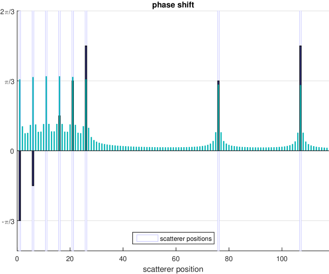
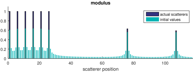
Figure 1: A number of $6$ equidistant scatterers on a periodic chain of length $117$. To allow for a signal from the substrate the wires are growing on we added some parasitic scatterers to the chain. As initial data we use the moduli and phases from $\mathbf{x}_{\mathrm{sparse}}$ symmetrically broadened by a leakage $\frac{1}{2}(\mathbf{f}_{0}^{+}+\mathbf{f}_{0}^{-})$, cf. (IV.8), with shift $s=0.3$ and amplitudes $0.6$ and $1.1$ respectively.

To demonstrate the relative phase recovery from the observed intensity (II.8) not only restricting to the Zinc-blende and Wurtzite phases (II.6) assume a linear chain with $117$ lattice sites and $6$ equidistant sparse amplitudes $|x_{j}|=1$ with phases from the set $\{-\frac{\pi}{3},-\frac{\pi}{6},0,\frac{\pi}{6},\frac{\pi}{3},\frac{\pi}{2}\}$ forming $\mathbf{x}_{\mathrm{sparse}}\in\mathbb{C}^{n}$.

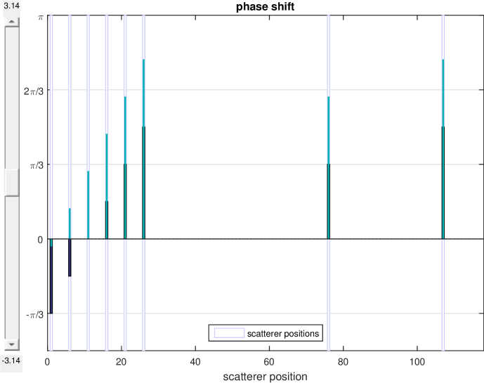
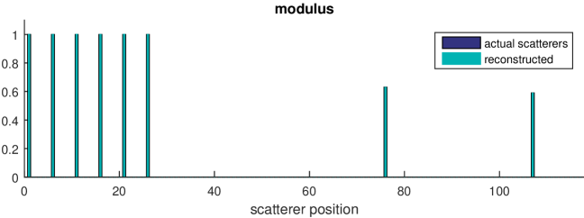
Figure 2: Reconstructed moduli of all scatterers. In the phase domain the values corresponding to vanishing moduli are suppressed. Due to the symmetry of the sensing problem the phases are only reconstructed up to a global phase.

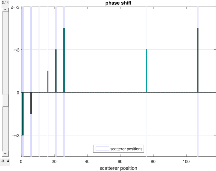
Figure 3: Adding a global phase (slider on the left) verifies that all relative phases are reconstructed correctly. The open rectangles mark the position of occupied lattice sites on the chain. In the original objective this would refer to bilayers and substrate in the nanowire.

As in the original objective the number of bilayers is roughly known we use as initial values $\mathbf{x}_{0}\in\mathbb{C}^{n}$ a broadened modulus and phase distribution related to the setting $\mathbf{x}_{\mathrm{sparse}}$, cf. Figure 1: With the support $\mathbb{S}:=\operatorname{supp}\mathbf{x}_{\mathrm{sparse}}$ a leakage

$$\big{(}\mathbf{f}^{\pm}_{0}\big{)}_{k}=\sum_{\alpha\in\mathbb{S}}\frac{\sin\big{(}(k\pm s-\alpha)\pi\big{)}}{(k\pm s-\alpha)\pi}\in\mathbb{R}\quad,\quad k=0,\ldots,n-1$$ (IV.8)

for the moduli and phases of $\mathbf{x}_{\mathrm{sparse}}$ is with shifts $0\leq s<1$ a suitable way to also consider the limit $s\to 0$ of exactly known positions. Note that for the phases we only used one fixed value for each occupied lattice site broadened by the leakage. So the main effort is the recovery of the relative phases from the measurements.

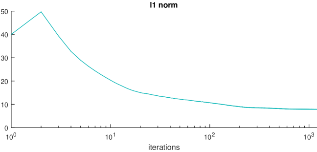
Figure 4: Note that the $\ell_{1}$ convergence (III.16) in the $k$th iteration step relates the linearized norm $\langle\mathbf{p}|\mathbf{x}_{k}\rangle\leq\left|\!\left|{\mathbf{x}_{k}}\right|\!\right|_{1}$ to $\left|\!\left|{\mathbf{x}_{k-1}}\right|\!\right|_{1}$. Because of this inequality, cf. (III.9), there is no guarantee of a monotonically lowered $\ell_{1}$ norm, which can be seen in the beginning (iteration step $2$).

For an exponential decaying lowering factor $\gamma_{k}=1-0.1\exp(-0.0019k)$ within $1200$ iterations the reconstruction results for noiseless synthetic measurements are shown in Figures 2 and 3. Experientially, good algorithm’s covariances were found to be

$$P_{0}=0.3\cdot\mathbbm{1}_{117}\;,\;Q=10^{-8}\cdot\mathbbm{1}_{117}\;,\;R=\operatorname{diag}(10^{-4},\ldots,10^{-4},10^{-6})\in\mathbb{R}^{118\times 118}$$ (IV.9)

To drive the $\ell_{1}$ minimization the corresponding entry (here $10^{-6}$) in the $R$ matrix has to be much lower in magnitude than the ones (here $10^{-4}$) related to the observations of the constraint. When reconstructed amplitudes are said to vanish (e.g. in Figure 2) this means only up to numerical precision where the zero value is dominated by the entries of $Q$. Empirically, the exponential decay in the lowering factor $\gamma_{k}$ is chosen such that its values approaches about $0.99,\ldots,0.999$ after the maximum number of iterations. A resulting typical smooth convergence of the $\ell_{1}$ norm due to the exponential decay is shown in Figure 4: The constant tail can be used to determine a maximal number of iterations as a stopping criterion. Note that the reconstructed results beyond this guessed number are insensitive to further iterations meaning for the equations (IV.5) to perform fixed point iterations within accuracies related to the covariances $Q$ and $P_{k}$.

In the nanowire the equidistant bilayers are at fixed positions in growth direction $\mathbf{a}_{3}$. Thus the reconstruction of their complex scattering amplitudes does not suffer from ‘off grid’ problems in general, see e.g. CSchPC11 ; DuBa13 ; TBSR13 , if integer multiples of the lattice constants are used for the DFT.

IV.2 Example 2: Pattern Reconstruction

The 2D reconstruction from (II.13) can be calculated with the same algorithm already used for Example 1 above, as the 2D data set of size $12\times 25$ can be mapped to a 1D vector by means of (II.14), cf. Figure 5. Like the example from Figure 1, we use as initial values with the same reasoning and broadening parameters the given distribution. Within $2000$ iterations and an exponentially decaying lowering factor $\gamma_{k}=1-0.17\cdot\exp(-0.0028k)$ the reconstruction for noiseless measurements is shown in Figure 6 with empirically good algorithm’s covariances

$$P_{0}=0.3\cdot\mathbbm{1}_{300}\;,\;Q=10^{-7}\cdot\mathbbm{1}_{300}\;,\;R=\operatorname{diag}(10^{-4},\ldots,10^{-4},10^{-6})\in\mathbb{R}^{301\times 301}\;\;.$$ (IV.10)

Note that there is a combined translational and reflectional symmetry mapping the vectorized real scattering amplitude distribution onto itself, cf. Figure 5. As this is also a symmetry of the squared observations (II.8) in the linear configuration, there are two competing solutions to the sensing problem. Interestingly, breaking this symmetry improved the $\ell_{1}$ convergence in Figure 6: Without the parasitic scatterers the symmetric positions of consecutive sites are correctly (with respect to the support) found after $5000$ iterations, cf. Figure 7, and the remaining discrepancies in the amplitudes do not even vanish completely after inefficient $50000$ iterations. On the contrary the random sample of $25$ scatterers from Figure 8 is already reconstructed with less than $1000$ iterations suggesting a strong dependence of the algorithm’s convergence from the vector under consideration.

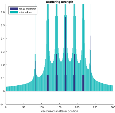
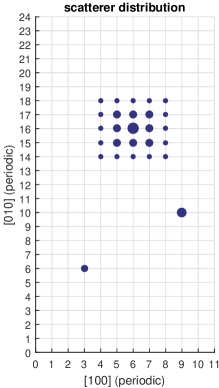
Figure 5: The actual scatterers forming the $5\times 5$ structure are made from real amplitudes $0.12$, $0.28$ and $0.56$ whereas the two parasitic scatterers are assigned with $0.23$ and $0.42$ (left panel). The scattering strength in the plane is represented by the area of the filled circles (right panel).

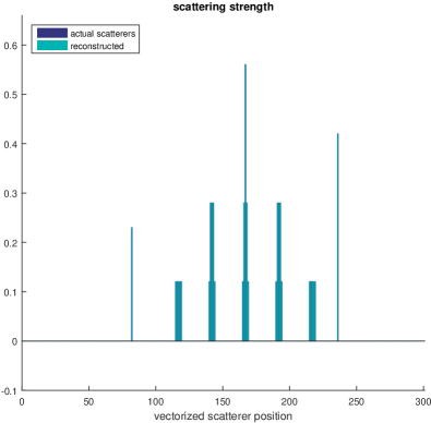
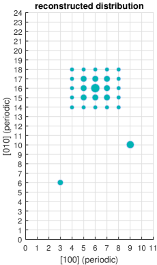
Figure 6: The real amplitudes are nicely reconstructed (left panel) after $2000$ iterations which can also be seen in the 2D setting (right panel) by comparing with Figure 5.

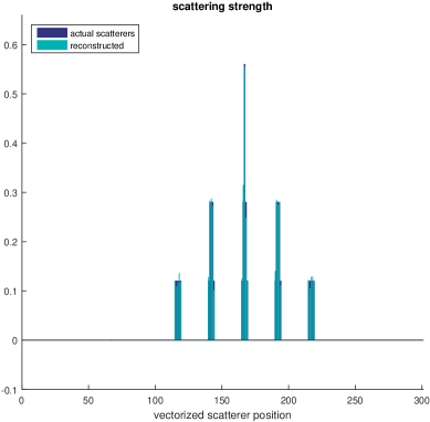
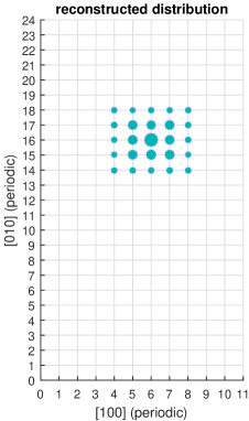
Figure 7: Without parasitic scatterers the positions are correctly found (right panel) after $5000$ iterations and $\gamma_{k}=1-0.17\cdot\exp(-0.0012k)$. The remaining discrepancies in the amplitudes seem to be complementarily symmetric with respect to the central peak (left panel).

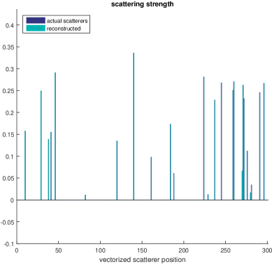
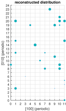
Figure 8: A random distribution of $25$ scatterers with real random amplitudes normalized in the $\ell_{2}$ norm. The reconstruction is without artefacts and discrepancies reached after $1000$ iterations with $\gamma_{k}=1-0.17\cdot\exp(-0.0058k)$.

V Conclusion and Outlook

We aimed to implement non-linear compressive sensing for complex vectors $\mathbf{x}$ by inverting the underlying observation model with Kalman filtering. For this reason we proved a weak convergence of the filter equations for complex sensing matrices $C$ and hermitian covariances $R,P,Q$. For the example of quadratic nonlinearities we applied our formulas to retrieve relative phase information in the objective of simulated noiseless coherent $X$​-ray diffraction. Due to the nonlinearity the noise in the intensity is not Gaussian and needs further considerations to also account for e.g. lattice distortions or the finite coherence of the primary beam. As an outlook we presented a 2D pattern reconstruction which, hopefully, can help to investigate if the cross sections of the wires were grown regularly.

Because of the Jacobians building up the sensing matrix $C$ the convergence of the underlying $\ell_{1}$ norm minimization does depend on the reconstructed vector $\mathbf{x}$ and may go beyond the resolution issues TBSR13 for even constant sensing matrices. For this reason a thorough analysis on the relation between maximal sparsity (for the examples here about 10% of the available lattice sites) and the Toeplitz matrix (II.9) representing the sensing process for a successful CS is needed. As mentioned in the introduction algorithms in general minimizing the $\ell_{1}$ norm could be of interest retrieving information out from intensity spectra: To compare our results we applied the non-linear version Valkonen14 of the primal dual algorithm ChPo10 to the 1D sensing problem above yielding similar results with respect to iteration numbers, reconstructed amplitudes and phases. On the one hand primal dual reconstructed the zeros outside the support (once a solution was isolated from the algorithm) numerically exact compared to accuracies of orders $10^{-5}$ reached by the Kalman filter. On the other hand our approach focused in the first quarter of the iterations on guessing the support by strongly increasing and decreasing the corresponding amplitudes, whereas primal dual homogeneously acted on all the amplitudes during all iterations. For a detailed comparison and maybe a combination, the whole parameter range of the approaches have to be investigated. To apply the Kalman filter-based algorithm above to recorded data DBLP16 we need to deal with several $10^{4}$ $\mathbf{x}$-vector’s entries describing a sparsely (by a factor of roughly $1:10^{1}$) occupied linear grid covering all the approximately $10^{3}$ bilayers in a nanowire of $500\,$nm in height. For this reason matrix inversions, cf. (IV.5), should be reformulated by e.g. sequential processing techniques to make the algorithm more scalable. Furthermore it would also be interesting if other adaptive lowering factors $\gamma_{k}$ compared to the exponential ones yield faster convergences.

As the reconstruction from quadratic constraints seems to depend only little on the explicit algorithm used for the $\ell_{1}$ minimization, it would be interesting to figure out to which extend the linear matrix completion approach CESV13 ; ChMoPa10 ; FoRaWa11 with respect to the nuclear norm can still be applied in face of seemingly too few numbers of independent observations.

Appendix A Vector Notations for Complex Numbers

Vectors over the field $\mathbb{C}$ consist of complex numbers $z=x+\mathrm{i}y$ with $x,y\in\mathbb{R}$ and $\mathrm{i}^{2}=-1$. With a vector $|\mathbf{v}\rangle\in\mathbb{C}^{n}$ we usually associate $n$ complex numbers $v_{1},v_{2},\ldots,v_{n}$ arranged as a column. With the complex conjugate $\overline{z}:=x-\mathrm{i}y$ row vectors $\langle\mathbf{v}|\in\mathbb{C}^{n}$ are considered to be dual to $|\mathbf{v}\rangle$ by

$$\begin{gathered}|\mathbf{v}\rangle=\begin{pmatrix}v_{1}\\ \vdots\\ v_{n}\end{pmatrix}\in\mathbb{C}^{n}\end{gathered}\quad,\quad\begin{aligned} \langle\mathbf{v}|:&=\big{(}\overline{v_{1}},\ldots,\overline{v_{n}}\big{)}\in\mathbb{C}^{n}\\ |\mathbf{v}\rangle&=\sum_{k=1}^{n}v_{k}|\mathbf{e}_{k}\rangle\;\;,\;\;\big{(}|\mathbf{v}\rangle\big{)}_{j}=v_{j}\in\mathbb{C}\end{aligned}$$ (A.1)

where $\big{(}|\mathbf{e}_{j}\rangle\big{)}_{k}=\delta_{jk}$ denotes with $j,k=1,\ldots,n$ the usual standard basis. With the complex scalar product

$$\langle\mathbf{v}|\mathbf{w}\rangle=\sum_{k=1}^{n}\overline{v_{k}}w_{k}\quad,\quad|\mathbf{v}\rangle,|\mathbf{w}\rangle\in\mathbb{C}^{n}$$ (A.2)

each vector $|\mathbf{v}\rangle\in\mathbb{C}^{n}$ can be represented in an unitary basis $\big{\{}|\mathbf{q}_{1}\rangle,\ldots,|\mathbf{q}_{n}\rangle\big{\}}\subset\mathbb{C}^{n}$ yielding the expansion

$$|\mathbf{v}\rangle=\sum_{k=1}^{n}|\mathbf{q}_{k}\rangle\langle\mathbf{q}_{k}|\mathbf{v}\rangle\quad,\quad\langle\mathbf{q}_{j}|\mathbf{q}_{k}\rangle=\delta_{jk}\text{ with }j,k=1,\ldots,n\quad.$$ (A.3)

With $A=(a_{ij})_{ij}\in\mathbb{C}^{m\times n}$ we denote matrices with $m$ rows and $n$ columns consisting of the complex entries $a_{ij}=(A)_{ij}$. Let $(A^{H})_{ij}:=\overline{(A)_{ji}}=\overline{a_{ji}}$ represent the hermitian conjugate then we get from its column decomposition $A^{H}=\big{(}|a_{1}\rangle,\ldots,|a_{n}\rangle\big{)}\in\mathbb{C}^{m\times n}$

$$A=\begin{pmatrix}\langle a_{1}|\\ \vdots\\ \langle a_{n}|\end{pmatrix}\quad,\quad\langle a_{j}|=|a_{j}\rangle^{H}\in\mathbb{C}^{m}\quad.$$ (A.4)

Using such a row decomposition the matrix multiplication of commensurable $A\in\mathbb{C}^{m\times n}$ and $B\in\mathbb{C}^{n\times p}$ can be viewed as $mp$ single scalar products yielding with $B=\big{(}|\mathbf{b}_{1}\rangle,\ldots,|\mathbf{b}_{p}\rangle\big{)}$

$$AB=C=(c_{ik})_{ik}\in\mathbb{C}^{m\times p}\quad,\quad c_{ik}=\sum_{\ell=1}^{n}a_{i\ell}b_{\ell k}=\langle\mathbf{a}_{i}|\mathbf{b}_{k}\rangle$$ (A.5)

including products $A|\mathbf{x}\rangle\in\mathbb{C}^{m}$ for $B=|\mathbf{x}\rangle\in\mathbb{C}^{n}$. Thus with the identity $\mathbbm{1}_{n}=(\delta_{ij})_{ij}\in\mathbb{C}^{n\times n}$ unitary matrices $Q=\big{(}|\mathbf{q}_{1}\rangle,\ldots,|\mathbf{q}_{n}\rangle\big{)}\in\mathbb{C}^{n\times n}$ consist of orthonormal (row and) columns defined by the property

$$QQ^{H}=Q^{H}Q=\mathbbm{1}_{n}\quad,\quad\big{(}Q^{H}Q\big{)}_{jk}=\langle\mathbf{q}_{j}|\mathbf{q}_{k}\rangle=\delta_{jk}\quad,\quad Q^{H}=Q^{-1}\quad.$$ (A.6)

The possibility of multiplying matrices $A=(a_{ij})_{ij}\in\mathbb{C}^{m\times n}$ and $B=(b_{rs})_{rs}\in\mathbb{C}^{p\times q}$ of arbitrary dimensions is covered by the Kronecker product

$$A\otimes B=\left(\begin{array}[]{c|c|c}\begin{smallmatrix}a_{11}b_{11}&\ldots&a_{11}b_{1q}\\[-1.72218pt] \vdots&\ddots&\vdots\\[2.15277pt] a_{11}b_{p1}&\ldots&a_{11}b_{pq}\end{smallmatrix}&\hskip 10.00002pt\ldots&\begin{smallmatrix}a_{1n}b_{11}&\ldots&a_{1n}b_{1q}\\[-1.72218pt] \vdots&\ddots&\vdots\\[2.15277pt] a_{1n}b_{p1}&\ldots&a_{1n}b_{pq}\end{smallmatrix}\\[10.76385pt] \hline\cr\vdots&\ddots&\vdots\\ \hline\cr\phantom{.}&&\phantom{.}\\[-12.91663pt] \begin{smallmatrix}a_{m1}b_{11}&\ldots&a_{m1}b_{1q}\\[-1.72218pt] \vdots&\ddots&\vdots\\[2.15277pt] a_{m1}b_{p1}&\ldots&a_{m1}b_{pq}\end{smallmatrix}&\ldots&\begin{smallmatrix}a_{mn}b_{11}&\ldots&a_{mn}b_{1q}\\[-1.72218pt] \vdots&\ddots&\vdots\\[2.15277pt] a_{mn}b_{p1}&\ldots&a_{mn}b_{pq}\end{smallmatrix}\end{array}\right)\in\mathbb{C}^{(mp)\times(nq)}\vspace*{1ex}$$ (A.7)

reading in components $\big{(}A\otimes B\big{)}_{(ir)(js)}=a_{ij}b_{rs}$ with multiple row and column indices $(ir)$ and $(js)$ respectively. For $|\mathbf{x}\rangle\in\mathbb{C}^{n}$, $|\mathbf{y}\rangle\in\mathbb{C}^{q}$ and $\lambda\in\mathbb{C}$ the Kronecker product meets

$$\big{(}\lambda A|\mathbf{x}\rangle\big{)}\otimes\big{(}B|\mathbf{y}\rangle\big{)}=\big{(}A|\mathbf{x}\rangle\big{)}\otimes\big{(}\lambda B|\mathbf{y}\rangle\big{)}=\lambda\big{(}A\otimes B\big{)}\big{(}|\mathbf{x}\rangle\otimes|\mathbf{y}\rangle\big{)}\quad.$$ (A.8)

Introducing the length of row or column vectors $\mathbf{x}\in\mathbb{C}^{n}$ can be accomplished with the $\ell_{p}$ norms $\left|\!\left|{\mathbf{x}}\right|\!\right|_{p}$ defined for all real $p>0$ by

$$\left|\!\left|{\mathbf{x}}\right|\!\right|_{p}^{p}:=\sum_{j=1}^{n}|x_{j}|^{p}\quad,\quad\left|\!\left|{\mathbf{x}}\right|\!\right|_{0}:=\operatorname{card}\{j\,|\,x_{j}\not=0,j=1,\ldots,n\}\quad.$$ (A.9)

Especially $\ell_{0}$ is no norm but can be viewed as the number of non-zero entries. The corresponding matrix norms of $A\in\mathbb{C}^{m\times n}$ can be related to the vector norms according to

$$\left|\!\left|{A}\right|\!\right|_{p}:=\sup_{\mathbf{x}\in\mathbb{C}^{n}}\frac{\left|\!\left|{A\mathbf{x}}\right|\!\right|_{p}}{\left|\!\left|{\mathbf{x}}\right|\!\right|_{p}}=\sup_{\left|\!\left|{\mathbf{x}}\right|\!\right|_{p}=1}\left|\!\left|{A\mathbf{x}}\right|\!\right|_{p}\quad.$$ (A.10)

Appendix B Hermitian Matrices

Hermitian matrices $X,Y\in\mathbb{C}^{n\times n}$ can be related by $X>Y$ ($X\geq Y$) if $X-Y$ is positive (semi) definite which can be written as $X-Y>0$ ($X-Y\geq 0$). In addition

Theorem Hackbusch93 .

If $X,Y\in\mathbb{C}^{n\times n}$ are hermitian with $X\geq Y>0$. Then $0<X^{-1}\leq Y^{-1}$.

Proof.

$Y=Y^{\frac{1}{2}}Y^{\frac{1}{2}}$, cf. § 9.2.4 in GoLo13 $\Rightarrow\mathbbm{1}_{n}\leq Y^{-\frac{1}{2}}XY^{-\frac{1}{2}}$ has eigenvalues larger than $1$ $\Rightarrow Y^{\frac{1}{2}}X^{-1}Y^{\frac{1}{2}}$ has positive eigenvalues lower than $1$ $\Rightarrow 0<Y^{\frac{1}{2}}X^{-1}Y^{\frac{1}{2}}\leq\mathbbm{1}_{n}$. ∎

Thus all hermitian matrices $R,X\in\mathbb{C}^{n\times n}$ with $R$ positive definite and $X$ positive semi definite satisfy the inequalities

$$R+X\geq R>0\quad\Leftrightarrow\quad 0<\big{(}R+X\big{)}^{-1}\leq R^{-1}$$ (B.1)

References

- (1) T. Akiyama, K. Nakamura, and T. Ito, Effects of stacking sequence on the electrical conductivity of InAs: A combination of density functional theory and Boltzmann transport equation calculations, Jap. J. Appl. Phys. 54 (2015), 075001.
- (2) E. P. A. M. Bakkers, M. T. Borgstrom, and M. A. Verheijen, Epitaxial growth of III-V nanowires on group IV substrates, MRS Bull. 32 (2007), 117.
- (3) M. Barchuk, V. Holý, D. Kriegner, J. Stangl, S. Schwaiger, and F. Scholz, Diffusive X-ray scattering from stacking faults in a-plane GaN epitaxial layers, Phys. Rev. B 84 (2011), 094113.
- (4) A. Biermanns, D. Carbone, S. Breuer, V. L. R. Jacques, T. Schulli, L. Geelhaar, and U. Pietsch, Distribution of zinc-blende twins and wurtzite segments in GaAs nanowires probed by X-ray nanodiffraction, Phys. stat. sol. RRL 7 (2013), 860.
- (5) Y. B. Bolkhovityanov and O. P. Pchelyakov, GaAs epitaxy on Si substrates: modern status of research and engineering, Phys.-Usp. 51 (2008), 437.
- (6) E. J. Candès, Y. Eldar, T. Strohmer, and V. Voroninski, Phase retrieval via matrix completion, SIAM J. Imaging Sci. 6 (2013), 199.
- (7) E. J. Candès, J. Romberg, and T. Tao, Stable signal recovery from incomplete and inaccurate measurements, Comm. Pure Appl. Math. 59 (2006), 1207.
- (8) A. Chai, M. Moscoso, and G. Papanicolaou, Array imaging using intensity-only measurements, Tech. report, Stanford University, 2010.
- (9) A. Chambolle and T. Pock, A First-Order Primal-Dual Algorithm for Convex Problems with Applications to Imaging, J. Math. Imag. Vis. 40 (2010), 120.
- (10) H. N. Chapman and K. A Nugent, Coherent lensless X-ray imaging, Nat. Phot. 4 (2010), 833.
- (11) S. S. Chen, D. L. Donoho, and M. A. Saunders, Atomic Decomposition by Basis Pursuit, SIAM Rev. 43 (2001), no. 1, 129.
- (12) Y. Chi, L. L. Scharf, A. Pezeshki, and A. R. Calderbank, Sensitivity to Basis Mismatch in Compressed Sensing, IEEE Trans. Signal Process. 59 (2011), 2182.
- (13) N. Correll, Introduction to Autonomous Robots, CreateSpace Independent Publishing Platform, 2014.
- (14) Y. Cui and C. M. Lieber, Functional nanoscale electronic devices assembled using silicon nanowire building blocks, Science 291 (2001), 851.
- (15) A. Davtyan, A. Biermanns, O. Loffeld, and U. Pietsch, Determination of the stacking fault density in highly defective single GaAs nanowires by means of coherent diffraction imaging, New J. Phys. 18 (2016), 063021.
- (16) D. L. Donoho, Compressed sensing, IEEE Trans. Inform. Theory 52 (2006), 1289.
- (17) X. F. Duan, Y. Huang, Y. Cui, J. F. Wang, and C. M. Lieber, Indium phosphide nanowires as building blocks for nanoscale electronic and optoelectronic devices, Nature 409 (2001), 66.
- (18) M. F. Duarte and R. Baraniuk, Spectral compressive sensing, Appl. Comput. Harmon. Anal. 35 (2013), 111.
- (19) V. Favre-Nicolin, J. Eymery, R. Koester, and P. Gentile, Coherent-diffraction imaging of single nanowires of diameter 95 nanometers, Phys. Rev. B 79 (2009), 195401.
- (20) J. R. Fienup, Reconstruction of an object from the modulus of its Fourier transform, Opt. Lett. 3 (1978), 27.
- (21) , Phase retrieval algorithms - a comparison, Appl. Opt. 21 (1982), 2758.
- (22) M. Fornasier, H. Rauhut, and R. Ward, Low-rank matrix recovery via iteratively reweighted least squares minimization, SIAM J. Optim. 21 (2011), 1614.
- (23) S. Foucart and H. Rauhut, A Mathematical Introduction to Compressive Sensing, Birkhäuser, 2013.
- (24) R. W. Gerchberg and W. O. Saxton, Practical algorithm for determination of phase from image and diffraction plane pictures, Optik 35 (1972), 237.
- (25) Gene H. Golub and Charles F. Van Loan, Matrix computations, John Hopkins, 2013.
- (26) M. S. Gudiksen, L. J. Lauhon, J. Wang, D. C. Smith, and C. M. Lieber, Growth of nanowire superlattice structures for nanoscale photonics and electronics, Nature 415 (2002), 617.
- (27) W. Hackbusch, Iterative Lösung großer schwachbesetzter Gleichungssysteme, p. 55 (Lemma 2.10.2), Teubner Verlag, 1993.
- (28) R. Horstmeyer, R. Y. Chen, X. Ou, B. Ames, J. A. Tropp, and C. Yang, Solving ptychography with a convex relaxation, New J. Phys. 17 (2015), 053044.
- (29) M. H. Huang, S. Mao, H. Feick, H. Q. Yan, Y. Y. Wu, H. Kind, E. Weber, R. Russo, and P. D. Yang, Room-temperature ultraviolet nanowire nanolasers, Science 292 (2001), 1897.
- (30) S. J. Julier and J. K. Uhlmann, New extension of the Kalman filter to nonlinear systems, AeroSense’97, International Society for Optics and Photonics, 1997, p. 182.
- (31) D. Kanevsky, A. Carmi, L. Horesh, P. Gurfil, B. Ramabhadran, and T. N. Sainath, Kalman Filtering for Compressed Sensing, The 13th International Conference on Information Fusion, 2010.
- (32) O. Loffeld, T. Espeter, and M. Heredia Conde, From weighted least squares estimation to sparse CS reconstruction, 3rd International Workshop on Compressed Sensing Theory and its Applications to Radar, Sonar and Remote Sensing (CoSeRa), 2015, p. 149.
- (33) P. S. Maybeck, Stochastic Models, Estimation and Control: Volume 1, Academic Press, 1979.
- (34) J. W. Miao, T. Ishikawa, I. K. Robinson, and M. M. Murnane, Beyond crystallography: Diffractive imaging using coherent X-ray light sources, Science 348 (2015), 530.
- (35) A. L. Patterson, A Fourier Series Method for the Determination of the Components of Interatomic Distances in Crystals, Phys. Rev. 46 (1934), 372.
- (36) P. M. Pelz, M. Guizar-Sicairos, P. Thibault, I. Johnson, M. Holler, and A. Menzel, On-the-fly scans for X-ray ptychography, Appl. Phys. Lett. 105 (2014), 251101.
- (37) I. Robinson and R. Harder, Coherent X-ray diffraction imaging of strain at the nanoscale, Nat. Mat. 8 (2009), 291.
- (38) H. L. Shi, B. Dong, and W. Z. Wang, Features of twins and stacking faults in silver nanorice and electron-beam irradiation effect, Nanoscale 4 (2012), 6389.
- (39) G. Tang, B. N. Bhaskar, P. Shah, and B. Recht, Compressed sensing off the grid, IEEE Trans. Inform. Theory 59 (2013), 7465.
- (40) T. Valkonen, A primal-dual hybrid gradient method for non-linear operators with applications to MRI, Inv. Prob. 30 (2014), 055012.
- (41) N. Vaswani, Kalman Filtered Compressed Sensing, Proc. IEEE Int. Conf. Image Process. (ICIP), 2008, p. 893.
- (42) B. E. Warren, X-Ray Diffraction, Dover Publications, 1990.