$\mathcal{H}$-matrix based second moment analysis for rough random fields and finite element discretizations

Abstract.

We consider the efficient solution of strongly elliptic partial differential equations with random load based on the finite element method. The solution’s two-point correlation can efficiently be approximated by means of an $\mathcal{H}$-matrix, in particular if the correlation length is rather short or the correlation kernel is non-smooth. Since the inverses of the finite element matrices which correspond to the differential operator under consideration can likewise efficiently be approximated in the $\mathcal{H}$-matrix format, we can solve the correspondent $\mathcal{H}$-matrix equation in essentially linear time by using the $\mathcal{H}$-matrix arithmetic. Numerical experiments for three-dimensional finite element discretizations for several correlation lengths and different smoothness are provided. They validate the presented method and demonstrate that the computation times do not increase for non-smooth or shortly correlated data.

1. Introduction

A lot of problems in science and engineering can be modeled in terms of strongly elliptic boundary value problems. While these problems are numerically well understood for input data which are given exactly, these input data are often only available up to a certain accuracy in practical applications, e.g., due to measurement errors or tolerances in manufacturing processes. In recent years, it has therefore become more and more important to take these inaccuracies in the input data into account and model them as random input parameters.

The Monte Carlo approach, see, e.g., [12] and the references therein, provides a straightforward approach to deal with these random data, but it has a relatively slow convergence rate which is only in the sense of the root mean square error. This, in turn, means that a large amount of samples has to be generated to obtain computational results with an acceptable accuracy, whereas the results still have a small probability of being too far away from the true solution. Therefore, in the past several years there have been presented multiple deterministic approaches to overcome this obstacle. For instance, random loads have been considered in [52, 57], random coefficients in [1, 2, 13, 18, 20, 42, 47, 49], and random domains in [36, 59].

For a domain $D\subset\mathbb{R}^{d}$ and a probability space $(\Omega,\mathcal{F},\mathbb{P})$, we consider the Dirichlet problem

(1) $$\left.\begin{aligned} \mathcal{L}u(\omega,{\bf x})&=f(\omega,{\bf x})&&\text{ for }{\bf x}\in D\\ u(\omega,{\bf x})&=0&&\text{ for }{\bf x}\in\Gamma\mathrel{\mathrel{\mathop{:}}=}\partial D\quad\end{aligned}\right\}\quad\text{$\mathbb{P}$-almost surely}$$

with random load $f(\omega,{\bf x})$ and a strongly elliptic partial differential operator $\mathcal{L}$ of second order.

We can compute the solution’s mean

$$\mathbb{E}_{u}({\bf x})\mathrel{\mathrel{\mathop{:}}=}\int_{\Omega}u(\omega,{\bf x})\operatorname{d}\!\mathbb{P}(\omega)$$

and also its two-point correlation

$$\operatorname{Cor}_{u}({\bf x},{\bf y})\mathrel{\mathrel{\mathop{:}}=}\int_{\Omega}u(\omega,{\bf x})u(\omega,{\bf y})\operatorname{d}\!\mathbb{P}(\omega)$$

if the respective quantities of the input data are known. Namely, the mean $\mathbb{E}_{u}$ satisfies

(2) $$\mathcal{L}\mathbb{E}_{u}=\mathbb{E}_{f}\text{ in }D\quad\text{and}\quad\mathbb{E}_{u}=0\text{ on }\Gamma$$

due to the linearity of the expectation and the differential operator $\mathcal{L}$. Taking into account the multi-linearity of the tensor product, one verifies by tensorizing (1) that

(3) $$(\mathcal{L}\otimes\mathcal{L})\operatorname{Cor}_{u} =\operatorname{Cor}_{f} \text{ in }D\times D,$$

$$(\mathcal{L}\otimes\operatorname{\operatorname{Id}})\operatorname{Cor}_{u} =0 \text{ on }D\times\Gamma,$$

$$(\operatorname{\operatorname{Id}}\otimes\mathcal{L})\operatorname{Cor}_{u} =0 \text{ on }\Gamma\times D,$$

$$\operatorname{Cor}_{u} =0 \text{ on }\Gamma\times\Gamma.$$

From $\operatorname{Cor}_{u}$, we can compute the variance $\mathbb{V}_{u}$ of the solution due to

$$\mathbb{V}_{u}(\mathbf{x})=\operatorname{Cor}_{u}(\mathbf{x},\mathbf{x})-\mathbb{E}_{u}(\mathbf{x})^{2}.$$

If a low-rank factorization of $\operatorname{Cor}_{f}$ is available, (3) can easily be solved by standard finite element methods. The existence of an accurate low-rank approximation is directly related to the spectral decomposition of the associated Hilbert-Schmidt operator

(4) $$(\mathcal{C}_{f}\psi)({\bf x})\mathrel{\mathrel{\mathop{:}}=}\int_{D}\operatorname{Cor}_{f}({\bf x},{\bf y})\psi({\bf y})\operatorname{d}\!{\bf y}.$$

Let $\operatorname{Cor}_{f}\in H^{p}(D)\otimes H^{p}(D)$, then, according to [26, 53], the eigenvalues of this Hilbert-Schmidt operator decay like

(5) $$\lambda_{m}\lesssim m^{-2p/d}\text{ as }m\rightarrow\infty.$$

Unfortunately, the constant in this estimate behaves similar to the $H^{p}(D)\otimes L^{2}(D)$-norm of $\operatorname{Cor}_{f}$. The following consideration shows that this can lead to large constants in the decay estimate if the correlation length is small. Let the correlation kernel $k(r)$ depend only on the distance $r=\|{\bf x}-{\bf y}\|$. Then, the derivatives $\partial_{\mathbf{x}}^{\boldsymbol{\alpha}}\operatorname{Cor}_{f}(\mathbf{x},\mathbf{y})$ and $\partial_{\mathbf{y}}^{\boldsymbol{\alpha}}\operatorname{Cor}_{f}(\mathbf{x},\mathbf{y})$ of the correlation

$$\operatorname{Cor}_{f}(\mathbf{x},\mathbf{y})=k\bigg{(}\frac{\|\mathbf{x-\mathbf{y}\|}}{\ell}\bigg{)},$$

involve the factor $\ell^{-|\boldsymbol{\alpha}|}$, leading to a constant $\ell^{-p}$ in the decay estimate of the eigenvalues (5). Thus, for a small correlation length $\ell$, a low-rank approximation of $\operatorname{Cor}_{f}$ becomes prohibitively expensive to compute.

Different approaches to tackle the solution of (3) have been considered in several articles, where most of them have in common that they are in some sense based on a sparse tensor product discretization of the solution. For example, the computation of the second moment, i.e., $\operatorname{Cor}_{u}$, has been considered for elliptic diffusion problems with random loads in [52] by means of a sparse tensor product finite element method. A sparse tensor product wavelet boundary element method has been used in [36] to compute the solution’s second moment for elliptic potential problems on random domains. In [32, 35], the computation of the second moment was done by multilevel finite element frames. Recently, this concept has been simplified by using the combination technique, cf. [34]. Unfortunately, the sparse tensor product discretization needs to resolve the concentrated measure for short correlation lengths. This means that the number of hierarchies of the involved finite element spaces has to be doubled if the correlation length is halved to get the same accuracy.

The present article discusses a different approach to approximate the full tensor product discretization without losing its resolution properties. In [14], it has been demonstrated that the $\mathcal{H}$-matrix technique is a powerful tool to cope with Dirichlet data of low Sobolev smoothness if the problem is formulated as a boundary value problem. There, the similar behavior of two-point correlation kernels and boundary integral operators has been exploited. In [15], $\mathcal{H}$-matrix compressibility of the solution was proven also in case of local operators on domains. In the present article, we will combine this theoretical foundation with the $\mathcal{H}$-matrix technique used in [14] to efficiently solve (3) by the finite element method for a right hand side $\operatorname{Cor}_{f}$ with small correlation length or low Sobolev smoothness.

The general concept of $\mathcal{H}$-matrices and the corresponding arithmetic have at first been introduced in [27, 29]. $\mathcal{H}$-matrices are feasible for the data-sparse representation of (block-) matrices which can be approximated block-wise with low-rank and have originally been employed for the efficient treatment of boundary integral equations as they arise in the boundary element method.

The rest of this article is organized as follows. In Section 2, we introduce the Galerkin discretization of the problem under consideration. Section 3 discusses the compressibility of discretized correlation kernels and the efficient solution of general correlation equations. In Section 4, we recall some specialities of $\mathcal{H}$-matrices in the context of finite elements. In particular, we restate a phenomenon, called “weak admissibility”, which produces a more data-sparse representation of the correlation matrices, and $\mathcal{H}$-matrix nested dissection techniques. In Section 5, we present numerical examples to validate and quantify the proposed method. Finally, in Section 6, we draw our conclusions from the theoretical findings and the numerical results.

2. Preliminaries

For the remainder of this article, let $D\subset\mathbb{R}^{d}$ be a Lipschitz domain, $(\Omega,\mathcal{F},\mathbb{P})$ a separable, complete probability space and $\mathcal{L}$ the linear differential operator of second order given by

(6) $$(\mathcal{L}u)({\bf x})\mathrel{\mathrel{\mathop{:}}=}-\operatorname{div}\big{(}\mathbf{A}(\mathbf{x})\cdot\nabla u(\mathbf{x})\big{)}+c(\mathbf{x})u(\mathbf{x}).$$

The differential operator shall be strongly elliptic in the sense that

$$\underline{\alpha}\|\boldsymbol{\xi}\|_{2}^{2}\leq\boldsymbol{\xi}^{\intercal}\mathbf{A}(\mathbf{x})\boldsymbol{\xi}\leq\overline{\alpha}\|\boldsymbol{\xi}\|_{2}^{2}\text{ for all }\boldsymbol{\xi}\in\mathbb{R}^{d}$$

with coefficients $\mathbf{A}\in W^{1,\infty}\big{(}D,\mathbb{R}^{d\times d}\big{)}$, $0\leq c\in L^{\infty}(D,\mathbb{R})$, and $0<\underline{\alpha}\leq\overline{\alpha}<\infty$.

Under these assumptions, for a given load $f\in L^{2}_{\mathbb{P}}\big{(}\Omega,H^{-1}(D)\big{)}$, the Dirichlet problem

$$\mathcal{L}u(\omega,{\bf x}) =f(\omega,{\bf x}) \text{ for }{\bf x}\in D$$

$$u(\omega,{\bf x}) =0 \text{ for }{\bf x}\in\Gamma\mathrel{\mathrel{\mathop{:}}=}\partial D,$$

is known to have a unique solution $u(\omega,\cdot)\in H_{0}^{1}(D)$ for $\mathbb{P}$-almost every $\omega\in\Omega$, cf., e.g., [21]. As a result, the mean $\mathbb{E}_{u}\in H_{0}^{1}(D)$ and the correlation $\operatorname{Cor}_{u}\in H_{0}^{1}(D)\otimes H_{0}^{1}(D)$ are well defined.

For the efficient numerical solution of (3), we use a finite element Galerkin scheme. To that end, we introduce a finite element space $V_{N}=\operatorname{span}\{\varphi_{1},\ldots,\varphi_{N}\}\subset H_{0}^{1}(D)$. It is assumed that the mesh which underlies this finite element space is quasi-uniform. The basis functions $\{\varphi_{i}\}_{i}$ are supposed to be locally and isotropically supported such that $\operatorname{diam}(\operatorname{supp}\varphi_{i})\sim N^{-1/d}$. In particular, we can assign to each degree of freedom $i\in\{1,\ldots,N\}$ a suitable point ${\bf x}_{i}\in D$, e.g., the barycenter of the support of the corresponding basis function or the corresponding Lagrangian interpolation point if nodal finite element shape functions are considered.

The variational formulation of (3) is given as follows:

$$\text{Find}\ \operatorname{Cor}_{u}\in H_{0}^{1}(D)\otimes H_{0}^{1}(D)\text{ such that }$$

$$\quad\big{(}(\mathcal{L}\otimes\mathcal{L})\operatorname{Cor}_{u},v\big{)}_{L^{2}(D\times D)}=(\operatorname{Cor}_{f},v)_{L^{2}(D\times D)}\text{ for all }v\in H_{0}^{1}(D)\otimes H_{0}^{1}(D).$$

By replacing the energy space $H_{0}^{1}(D)\otimes H_{0}^{1}(D)$ in this variational formulation by the finite dimensional ansatz space $V_{N}\otimes V_{N}$, we arrive at

(7) $$\text{Find}\ \operatorname{Cor}_{u,N}\in V_{N}\otimes V_{N}\text{ such that }$$

$$\quad\big{(}(\mathcal{L}\otimes\mathcal{L})\operatorname{Cor}_{u,N},v\big{)}_{L^{2}(D\times D)}=(\operatorname{Cor}_{f},v)_{L^{2}(D\times D)}\text{ for all }v\in V_{N}\otimes V_{N}.$$

A basis in $V_{N}\otimes V_{N}$ is formed by the set of tensor product basis functions $\{\varphi_{i}\otimes\varphi_{j}\}_{i,j}$. Hence, representing $\operatorname{Cor}_{u,N}$ by its basis expansion, yields

$$\operatorname{Cor}_{u,N}=\sum_{\ell,\ell^{\prime}=1}^{N}u_{\ell,\ell^{\prime}}(\varphi_{\ell}\otimes\varphi_{\ell^{\prime}}).$$

Setting ${\bf C}_{u}\mathrel{\mathrel{\mathop{:}}=}[u_{\ell,\ell^{\prime}}]_{\ell,\ell^{\prime}}$, we end up with the linear system of equations

(8) $$({\bf A}\otimes{\bf A})\operatorname{\operatorname{vec}}({\bf C}_{u})=\operatorname{\operatorname{vec}}({\bf C}_{f}),$$

where ${\bf C}_{f}\mathrel{\mathrel{\mathop{:}}=}\big{[}(\operatorname{Cor}_{f},\varphi_{\ell}\otimes\varphi_{\ell^{\prime}})_{L^{2}(D\times D)}\big{]}_{\ell,\ell^{\prime}}$ is the discretized two-point correlation of the Dirichlet data $f$ and ${\bf A}\mathrel{\mathrel{\mathop{:}}=}\big{[}(\mathcal{L}\varphi_{\ell^{\prime}},\varphi_{\ell})_{L^{2}(D)}\big{]}_{\ell,\ell^{\prime}}$ is the system matrix of the second order differential operator (6). In (8), the tensor product has, as usual in connection with matrices, to be understood as the Kronecker product. Furthermore, for a matrix ${\bf B}=[{\bf b}_{1},\ldots,{\bf b}_{n}]\in\mathbb{R}^{m\times n}$, the operation $\operatorname{\operatorname{vec}}({\bf B})$ is defined as

$$\operatorname{\operatorname{vec}}([{\bf b}_{1},\ldots,{\bf b}_{n}])\mathrel{\mathrel{\mathop{:}}=}\begin{bmatrix}{\bf b}_{1}\\ \vdots\\ {\bf b}_{n}\end{bmatrix}\in\mathbb{R}^{mn}.$$

For matrices ${\bf B}\in\mathbb{R}^{k\times n}$, ${\bf C}\in\mathbb{R}^{\ell\times m}$ and ${\bf X}\in\mathbb{R}^{m\times n}$, there holds the relation

$$({\bf B}\otimes{\bf C})\operatorname{\operatorname{vec}}({\bf X})=\operatorname{\operatorname{vec}}({\bf CXB}^{\intercal}).$$

Hence, we may rewrite (8) according to

(9) $${\bf A}{\bf C}_{u}{\bf A}^{\intercal}={\bf C}_{f}.$$

An approach to deal with non-homogeneous boundary conditions has been presented in [32].

3. $\mathcal{H}$-matrix approximation of correlation kernels

The matrix equation (9) has $N^{2}$ unknowns and is therefore not directly solvable if $N$ is large due to memory and time consumption. Thus, an efficient compression scheme and a powerful arithmetic are needed to obtain its solution. In the following, we will restrict ourselves to asymptotically smooth correlation kernels $\operatorname{Cor}_{f}$, i.e., correlation kernels satisfying the following definition.

Definition 3.1.

Let $k\colon\mathbb{R}^{d}\times\mathbb{R}^{d}\to\mathbb{R}$. The function $k$ is called asymptotically smooth if for some constants $c_{1},c_{2}>0$ and $q\in\mathbb{R}$ holds

(10) $$\big{|}\partial_{\bf x}^{\boldsymbol{\alpha}}\partial_{\bf y}^{\boldsymbol{\beta}}k({\bf x},{\bf y})\big{|}\leq c_{1}\frac{(|\boldsymbol{\alpha}|+|\boldsymbol{\beta}|)!}{c_{2}^{{|\boldsymbol{\alpha}|+|\boldsymbol{\beta}|}}}\|{\bf x}-{\bf y}\|_{2}^{-d-2q-|\boldsymbol{\alpha}|-|\boldsymbol{\beta}|},\quad\mathbf{x}\neq\mathbf{y},$$

independently of ${\boldsymbol{\alpha}}$ and ${\boldsymbol{\beta}}$.

Examples for asymptotically smooth correlation kernels are the Matérn kernels, which include especially the Gaussian kernel, cf. [46, 50] and the references therein. A main feature of such asymptotically smooth correlation kernels is that they exhibit a data-sparse representation by means of $\mathcal{H}$-matrices, cf., e.g., [6, 8, 28].

$\mathcal{H}$-matrices rely on local low-rank approximations of a given matrix ${\bf X}\in\mathbb{R}^{N\times N}$. For suitable non-empty index sets $\nu,\nu^{\prime}\subset\{1,\ldots,N\}$, a matrix block ${\bf X}|_{\nu\times\nu^{\prime}}$ can be approximated by a rank-$k$ matrix. This approximation can be represented in factorized form ${\bf X}|_{\nu\times\nu^{\prime}}\approx{\bf YZ}^{\intercal}$ with factors ${\bf Y}\in\mathbb{R}^{\nu\times k}$ and ${\bf Z}\in\mathbb{R}^{\nu^{\prime}\times k}$. Hence, if $k\ll\min\{\#\nu,\#\nu^{\prime}\}$, the complexity for storing the block is considerably reduced. The construction of the index sets is based on the cluster tree.

3.1. Cluster tree

For a tree $\mathcal{T}=(V,E)$ with vertices $V$ and edges $E$, we define its set of leaves by

$$\mathcal{L}(\mathcal{T})\mathrel{\mathrel{\mathop{:}}=}\{\sigma\in V\colon\sigma~{}\text{has no sons}\}.$$

Furthermore, we say that $\mathcal{T}$ is a cluster tree for the set $\{1,\ldots,N\}$ if the following conditions hold.

• $\{1,\ldots,N\}$ is the root of $\mathcal{T}$.

• All $\sigma\in V\setminus\mathcal{L}(\mathcal{T})$ are the disjoint union of their sons.

The level of $\sigma\in\mathcal{T}$ is its distance of the root, i.e., the number of son relations that are required for traveling from $\{1,\ldots,N\}$ to $\sigma$. We define the set of clusters on level $j$ as

$$\mathcal{T}^{(j)}:=\{\sigma\in\mathcal{T}\colon\sigma~{}\text{has level}~{}j\}.$$

The construction of the cluster tree is based on the support of the clusters. The support $\Upsilon_{\sigma}$ of a cluster $\sigma$ is defined as the union of the supports of the basis functions corresponding to their elements, that is

$$\Upsilon_{\sigma}=\bigcup_{i\in\sigma}\Upsilon_{i}\text{ where}\ \Upsilon_{i}:=\operatorname{supp}\varphi_{i}\ \text{for all}\ i\in\{1,\ldots,N\}.$$

For computing complexity bounds, the cluster tree should match the following additional requirements, uniformly as $N\to\infty$:

• The cluster tree is a balanced tree in the sense that the maximal level satisfies $J\sim\log_{2}N$.

• The diameter of the support $\Upsilon_{\sigma_{j}}$, $\sigma_{j}\in\mathcal{T}^{(j)}$, is local with respect to the level $j$, i.e., $\operatorname{diam}\Upsilon_{\sigma_{j}}\sim 2^{-j/d}$. Moreover, the number $\#\sigma_{j}$ of indices contained in a cluster $\sigma_{j}\in\mathcal{T}^{(j)}$ scales approximately like $2^{J-j}$, i.e., $\#\sigma_{j}\sim 2^{J-j}$.

Until further notice, a binary cluster tree $\mathcal{T}$ with the indicated terms should be given for our further considerations. A common algorithm for its construction is based on a hierarchical subdivision of the point set which is associated with the basis functions, cf., e.g., [6, 8, 28]. We begin by embedding the point set $\{\mathbf{x}_{1},\ldots,\mathbf{x}_{N}\}$ in a top-level bounding-box. This bounding-box is subsequently subdivided into two cuboids of the same size where the corresponding clusters are described by the points in each bounding-box. This process is iterated until a bounding-box encloses less than a predetermined number of points.

3.2. $\mathcal{H}$-Matrix approximation

$\mathcal{H}$-matrices have originally been invented in [27, 29] and are a generalization of cluster techniques for the rapid solution of boundary integral equations such as the fast multipole method [25], the mosaic skeleton approximation [56], or the adaptive cross approximation [3].

For the discretization of an asymptotically smooth correlation, we introduce a partition of its domain of definition which separates smooth and non-smooth areas of the kernel function. It is based on the following

Definition 3.2.

Two clusters $\sigma$ and $\sigma^{\prime}$ are called $\eta$-admissible if

(11) $$\max\{\operatorname{diam}(\Upsilon_{\sigma}),\operatorname{diam}(\Upsilon_{\sigma^{\prime}})\}\leq\eta\,\operatorname{dist}(\Upsilon_{\sigma},\Upsilon_{\sigma^{\prime}})$$

holds for some fixed $\eta>0$.

We can obtain the set of admissible blocks by means of a recursive algorithm: Starting with the root $(\sigma_{0,0},\sigma_{0,0})$, the bounding-boxes of the current cluster pair are checked for admissibility. If they are admissible, the cluster pair is added to the set $\mathcal{F}$ which corresponds to the correlation kernel’s farfield. Otherwise, the admissibility check will be performed on all bounding-boxes of the possible pairs of son clusters of the two original clusters. When we arrive at a pair of leaf clusters with inadmissible bounding-boxes, the clusters are added to the set $\mathcal{N}$ which corresponds to the correlation kernel’s nearfield. The set $\mathcal{B}=\mathcal{F}\cup\mathcal{N}$ obviously inherits a tree structure from the recursive construction of $\mathcal{F}$ and $\mathcal{N}$ and is called the block cluster tree, see [6, 8, 28].

With the definition of the block cluster tree at hand, we are finally in the position to introduce $\mathcal{H}$-matrices.

Definition 3.3.

The set $\mathcal{H}(\mathcal{B},k)$ of $\mathcal{H}$-matrices of maximal block rank $k$ is defined according to

$$\mathcal{H}(\mathcal{B},k):=\big{\{}{\bf X}\in\mathbb{R}^{N\times N}:\operatorname{rank}\big{(}{\bf X}|_{\sigma\times\sigma^{\prime}}\big{)}\leq k\text{ for all }\big{(}\sigma,\sigma^{\prime}\big{)}\in\mathcal{F}\big{\}}.$$

Note that all nearfield blocks ${\bf X}|_{\sigma\times\sigma^{\prime}}$, $(\sigma,\sigma^{\prime})\in\mathcal{N}$, are allowed to be full matrices.

In accordance with [6, 8, 28], the storage cost of an $\mathcal{H}$-matrix ${\bf X}\in\mathcal{H}(\mathcal{B},k)$ is $\mathcal{O}(kN\log N)$. Here, for asymptotically smooth correlation kernels, the rank $k$ depends poly-logarithmically on the desired approximation accuracy $\varepsilon$, which in turn depends usually on the degrees of freedom $N$. These remarks pertain to the approximation of an explicitly given, asymptotically smooth correlation kernel $k$, such as $\operatorname{Cor}_{f}$ in (3).

The compressibility of an implicitly given correlation kernel, such as $\operatorname{Cor}_{u}$ in (3), has been studied in [15] for the case of smooth domains $D$. We restate the main theorem for the setting of the present article which employs that the Hilbert-Schmidt operator (4), related with the correlation kernel $\operatorname{Cor}_{f}$, is in general a pseudo-differential operator, see, e.g., [38, 39, 40, 55] and the references therein.

Theorem 3.4.

In the domain $D$ with analytic boundary $\partial D$, assume that the correlation kernel $\operatorname{Cor}_{f}$ in (3) gives rise to an operator $\mathcal{C}_{f}\in OPS^{\theta}_{cl,s}$, i.e., to a classical pseudo-differential operator with symbol $a_{f}(\mathbf{x},\boldsymbol{\xi})$ of order $\theta$ and of Gevrey class $s\geq 1$ in the sense of [10, Def. 1.1]. Assume further that the coefficients of the differential operator $\mathcal{L}$ are smooth. Then, the correlation kernel $\operatorname{Cor}_{u}$ of (3) is the Schwartz kernel of an operator $\mathcal{C}_{u}\in OPS^{\theta-4}_{cl,s}$.

Moreover, the kernel $\operatorname{Cor}_{u}(\mathbf{x},\mathbf{y})$ of the correlation operator $\mathcal{C}_{u}$ is smooth in $D\times D$ outside of the diagonal $\Delta:=\{(\mathbf{x},\mathbf{y})\in D\times D:\mathbf{x}=\mathbf{y}\}$ and there holds the pointwise estimate

(12) $$\qquad\qquad|\partial^{\boldsymbol{\alpha}}_{\mathbf{x}}\partial^{\boldsymbol{\beta}}_{\mathbf{y}}\operatorname{Cor}_{u}({\bf x},{\bf y})|\leq c\mathscr{A}^{|\boldsymbol{\alpha}+\boldsymbol{\beta}|}(|\boldsymbol{\alpha}|!)^{s}\boldsymbol{\beta}!\|{\bf x}-{\bf y}\|_{2}^{-\theta-d-|\boldsymbol{\alpha}|-|\boldsymbol{\beta}|+4}$$

for all $\boldsymbol{\alpha},\boldsymbol{\beta}\in\mathbb{N}_{0}^{d}$, $({\bf x},{\bf y})\in(D\times D)\backslash\Delta$ with some constants $c$ and $\mathscr{A}$ which depend only on $D$ and on $a_{f}$.

Obviously, for $s=1$, estimate (12) directly implies condition (10) for the asymptotic smoothness of $\operatorname{Cor}_{u}$, allowing us to approximate $\operatorname{Cor}_{u}$ by the means of $\mathcal{H}$-matrices. In particular, [15] provides also some numerical evidence that this result could likely be extended to Lipschitz domains.

An example of correlation kernels for $\operatorname{Cor}_{f}$ satisfying the condition of this theorem for $s\geq 1$ is the Matérn class of kernels. We refer to [15] for more details on how to verify the assumptions of the theorem for other correlation kernels.

3.3. $\mathcal{H}$-Matrix arithmetic and iterative solution

An important feature of $\mathcal{H}$-matrices is that efficient algorithms for approximate matrix arithmetic operations are available. For two $\mathcal{H}$-matrices ${\bf H}_{1},{\bf H}_{2}\in\mathcal{H}(\mathcal{B},k)$, the approximate matrix-matrix addition ${\bf H}_{1}{\text{\tt+}}{\bf H}_{2}\in\mathcal{H}(\mathcal{B},k)$ can be performed in $\mathcal{O}(k^{2}N\log N)$ operations while the approximate matrix-matrix multiplication ${\bf H}_{1}{\text{\tt*}}{\bf H}_{2}\in\mathcal{H}(\mathcal{B},k)$ can be performed in $\mathcal{O}(k^{2}N\log^{2}N)$ operations. Both of these operations are essentially block matrix algorithms with successive recompression schemes. Moreover, employing the recursive block structure, the approximate inversion or the approximate computation of the $LU$-decomposition within $\mathcal{H}(\mathcal{B},k)$ can also be performed in only $\mathcal{O}(k^{2}N\log^{2}N)$ operations. We refer the reader to [6, 8, 23, 28, 29] for further results and implementation details. Especially, the parallelization of the $\mathcal{H}$-matrix arithmetic and the $\mathcal{H}$-LU-decomposition has been discussed in [43, 44].

In the context of correlation equations, this approximate $\mathcal{H}$-matrix arithmetic has successfully been used in [14] to solve a problem, similar to (3), which has been discretized by the boundary element method. Then, the matrix $\mathbf{A}$ in (9) corresponds to the stiffness matrix from the boundary element method which can naturally be approximated by the $\mathcal{H}$-matrix technique. The resulting matrix equation has been solved using an iterative solver based on iterative refinement, cf. [22, 48, 58], which we are also going to employ here. This method has originally been introduced in [58] for the improvement of solutions to linear systems of equations based on the LU-factorization.

Having all matrices in (9) represented by $\mathcal{H}$-matrices, the solution can then be approximated as follows. Let ${\bf A}\approx\hat{\bf L}\hat{\bf U}$, where $\hat{\bf L},\hat{\bf U}\in\mathcal{H}(\mathcal{B},k)$, be an approximate LU-decomposition to ${\bf A}$, e.g., computed from $\mathbf{A}$ by the $\mathcal{H}$-matrix arithmetic. Starting with the initial guess ${\bf C}_{u}^{(0)}=\hat{\bf U}^{-1}\hat{\bf L}^{-1}{\bf C}_{f}\hat{\bf L}^{-\intercal}\hat{\bf U}^{-\intercal},$ we iterate

(13) $${\boldsymbol{\Theta}}^{(i)}={\bf C}_{f}-{\bf A}{\bf C}_{u}^{(i)}{\bf A}^{\intercal},\quad{\bf C}_{u}^{(i+1)}={\bf C}_{u}^{(i)}+\hat{\bf U}^{-1}\hat{\bf L}^{-1}{\boldsymbol{\Theta}}^{(i)}\hat{\bf L}^{-\intercal}\hat{\bf U}^{-\intercal},\quad i=0,1,\ldots.$$

Note that we use, in contrast to [14], the LU-decomposition with forward and backward substitution algorithms which avoids the expensive computation of an approximate inverse. Whether we use an approximate inverse as in [14] or an approximate LU-decomposition, the idea of the iterative refinement stays the same: The residual ${\boldsymbol{\Theta}}^{(i)}$ is computed with a higher precision than the correction $\hat{\bf U}^{-1}\hat{\bf L}^{-1}{\boldsymbol{\Theta}}^{(i)}\hat{\bf L}^{-\intercal}\hat{\bf U}^{-\intercal}$. This yields an improved approximation to the solution in each step. Note that this algorithm also algebraically coincides with an undamped preconditioned Richardson iteration, see, e.g., [51].

In the following, we will elaborate how this approach can be realized in the context of the finite element method. If $\mathbf{A}$ is symmetric and positive definite, the LU-decomposition could also be replaced by a Cholesky decomposition. Nonetheless, we will see in the numerical experiments that the computation time of the decomposition is negligible compared to the overall computation time and we prefer to stay in the more general, i.e. non-symmetric, setting.

4. $\mathcal{H}$-matrices in the context of finite elements

Although a finite element matrix has a sparse structure, its inverse and both factors of its LU-decomposition are generally fully populated. Nevertheless, the inverse and the LU-decomposition exhibit a data-sparse structure in the sense that they are $\mathcal{H}$-matrix compressible. We recall the main concepts from the literature, see, e.g., [4, 7, 16, 17, 28].

4.1. General concepts

A rough argument for the $\mathcal{H}$-matrix compressibility of the inverse makes use of the Green’s function $G$ of $\mathcal{L}$. Let $\delta_{\mathbf{x}}$ denote the Dirac distribution at the point $\mathbf{x}$ and let $G\colon\mathbb{R}^{d}\times\mathbb{R}^{d}\rightarrow\mathbb{R}$ satisfy

$$\mathcal{L}_{\mathbf{y}}G(\mathbf{x},\mathbf{y})=\delta_{\mathbf{x}}\text{ and }G(\cdot,\mathbf{y})|_{\Gamma}=0.$$

Then, the solution of

$$\mathcal{L}u({\bf x}) =f({\bf x}) \text{ for }{\bf x}\in D,$$

$$u({\bf x}) =0 \text{ for }{\bf x}\in\Gamma,$$

can be represented by

$$u(\mathbf{x})=(\mathcal{L}^{-1}f)(\mathbf{x})=\int_{D}G(\mathbf{x},\mathbf{y})f(\mathbf{y})\operatorname{d}\!\mathbf{y},\quad\mathbf{x}\in D.$$

If the Green’s function is analytic away from the diagonal, e.g., in the case of constant coefficients of $\mathcal{L}$, we can approximate the Green’s function away from the diagonal by local expansions of the kind

$$G(\mathbf{x},\mathbf{y})\approx\sum_{i=1}^{k}a(\mathbf{x})b(\mathbf{y}),$$

which is the theoretical basis for an $\mathcal{H}$-matrix approximation, see [6, 8, 28].

However, one of the advantages of the finite element method is that it can be applied also in case of non-constant coefficients. In [7], a proof was presented to guarantee the existence of an $\mathcal{H}$-matrix approximation to the inverse of the finite element stiffness matrix even in the case of essentially bounded diffusion coefficients and the other coefficients set to zero. This result was then extended in [4] to allow all coefficients to be only essentially bounded, providing the theoretical foundation for an $\mathcal{H}$-matrix approximation to the inverse of the differential operator from (6). Having the $\mathcal{H}$-matrix approximability of the inverse to the finite element matrix available, the approximability of the LU-decomposition to the finite element matrix has then been proven in [5].

While these first results hold up to the finite element discretization error, the results have recently been improved in [16, 17] to hold without additional error.

It remains to explain how to actually compute an $\mathcal{H}$-matrix approximation to the inverse or the LU-decomposition of a finite element stiffness matrix. To that end, note that a necessary condition for an entry $\mathbf{A}_{ij}$ in the finite element matrix to be non-zero is that $\Upsilon_{i}\cap\Upsilon_{j}\neq\emptyset$, i.e., the intersection of the corresponding supports of the basis functions is non-empty. This yields together with the $\eta$-adminissibility condition (11) that all entries of a finite element matrix have $\eta$-inadmissible supports, i.e., they are contained in the nearfield of an $\mathcal{H}$-matrix. A sparse finite element matrix can therefore be represented as an $\mathcal{H}$-matrix by reordering the index set corresponding to the clustering scheme introduced in Section 3.1 and inserting the non-zero entries into the nearfield. An illustration of this procedure can be found in Figure 1.

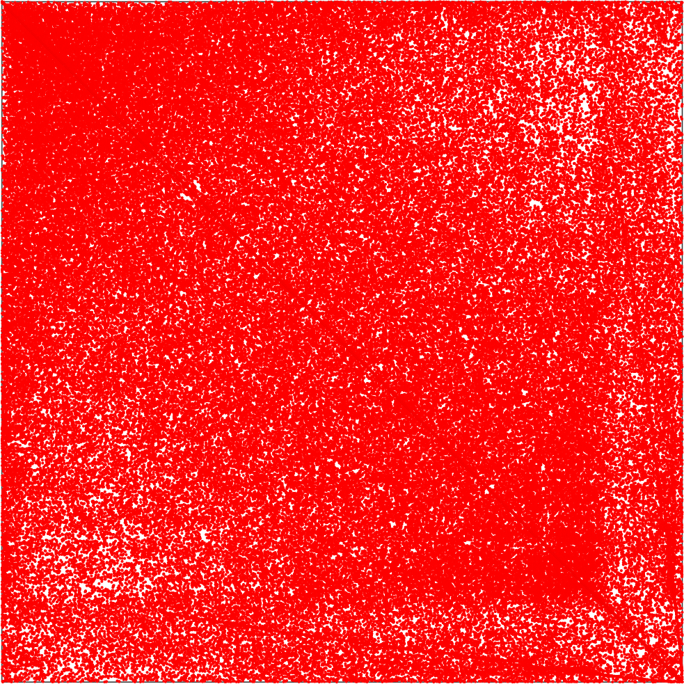
sparse FEM-matrix

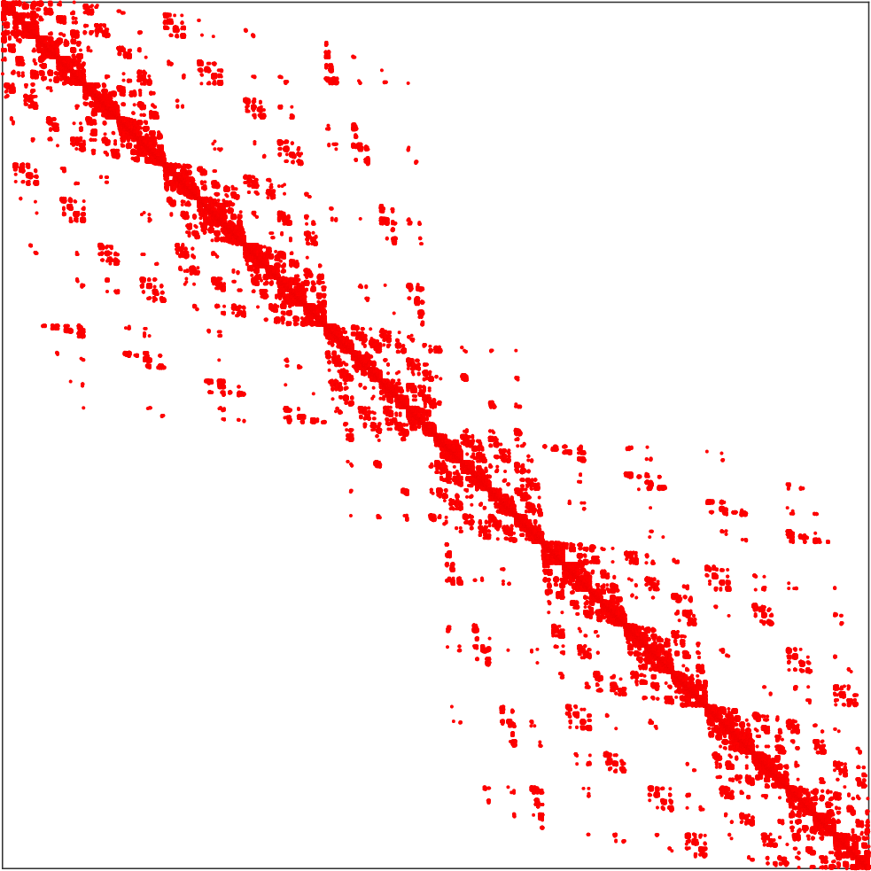
reordered FEM-matrix

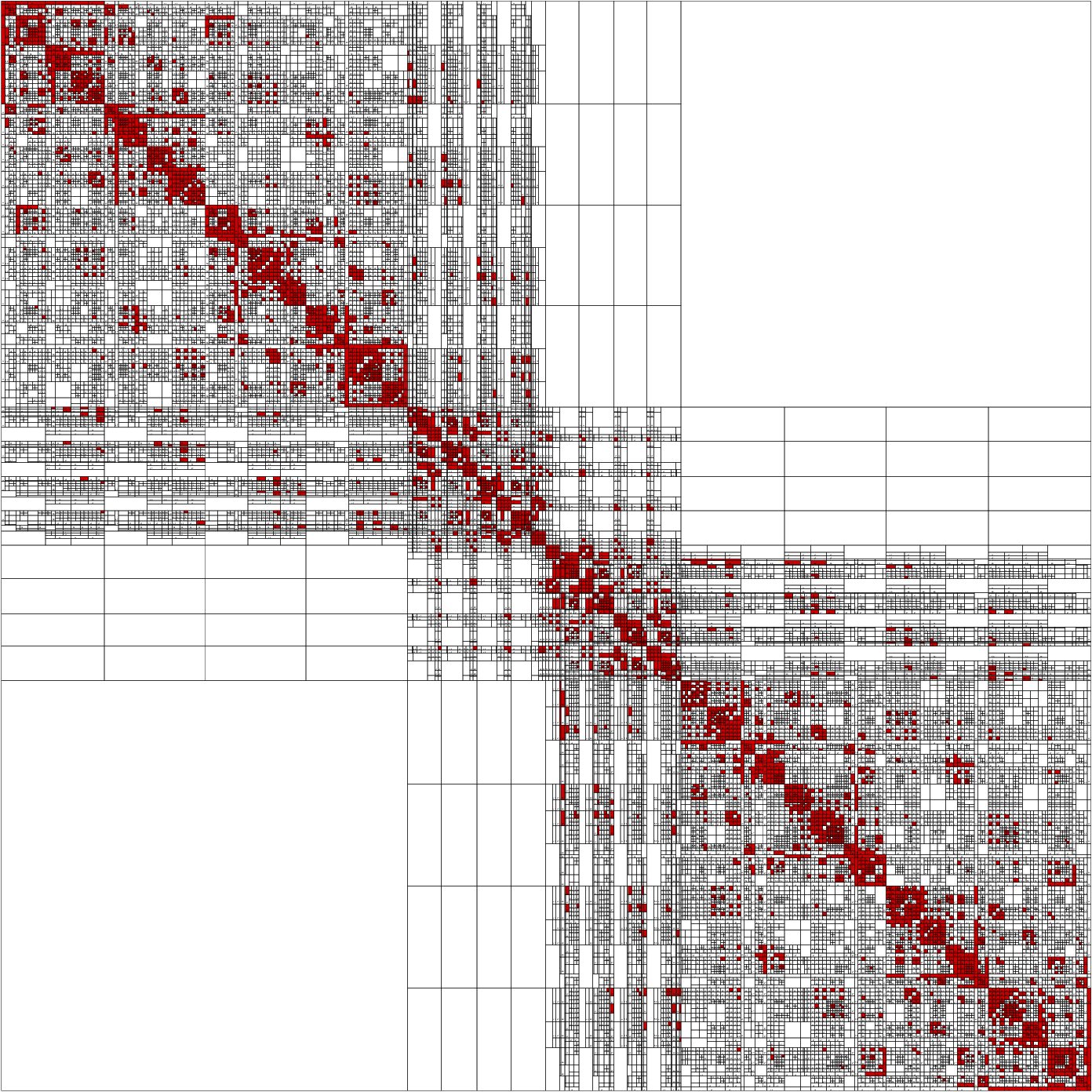
$\mathcal{H}$-matrix representation

Figure 1. Sparsity pattern of a 3D finite element matrix, its reordered finite element matrix, and the corresponding $\mathcal{H}$-matrix. Red blocks in the $\mathcal{H}$-matrix correspond to the nearfield, white blocks correspond to the empty farfield.

Having the finite element matrix represented by an $\mathcal{H}$-matrix, the approximate inverse and the LU-decomposition can be computed by using the block algorithms of the $\mathcal{H}$-matrix arithmetic in $\mathcal{O}(k^{2}N\log^{2}N)$ operations, cf. [6, 8, 28]. We note especially that the computation of the LU-decomposition together with its forward and backward substitution algorithms still have an overall complexity of $\mathcal{O}(k^{2}N\log^{2}N)$, but with smaller constants than the computation and the application of an approximate inverse.

4.2. Weak admissibility

Approximate $\mathcal{H}$-matrix representations for the inverse or LU-factorizations of finite element matrices have been used to construct preconditioners for iterative solvers, see, e.g., [6] and the references therein. In [30], it was observed for the one-dimensional case that the computation of an approximate inverse can be considerably sped up by replacing the $\eta$-admissibility condition (11) by the following weak admissibility condition.

Definition 4.1.

Two clusters $\sigma$ and $\sigma^{\prime}$ are called weakly admissible if $\sigma\neq\sigma^{\prime}$.

We observe immediately that an $\eta$-admissible block cluster is also weakly admissible. Thus, by replacing the $\eta$-admissibility condition by the weak admissibility, we obtain a much coarser partition of the $\mathcal{H}$-matrix. This leads to smaller constants in the storage and computational complexity, cf. [30]. Each row and each column of the finite element matrix has only $\mathcal{O}(1)$ entries. Thus, inserting the finite element matrix into a weakly admissible $\mathcal{H}$-matrix structure, the off-diagonal blocks of the $\mathcal{H}$-matrix have low-rank.

By partitioning the matrix according to the weak admissibility condition, we cannot ensure the exponential convergence of fast black box low-rank approximation techniques as used for boundary element matrices. For example, the adaptive cross approximation (ACA) relies on an admissibility condition similar to (11) to ensure exponential convergence, cf. [3]. Instead, the authors of [30] suggest to assemble a weakly admissible matrix block according to the $\eta$-admissibility condition and transform it on-the-fly to a low-rank matrix to obtain a good approximation.

The behavior of the ranks of the low-rank matrices in weakly admissible partitions compared to $\eta$-admissible partitions is not fully understood yet. Suppose that $k_{\eta}$ is an upper bound for the ranks corresponding to an $\eta$-admissible partition and suppose that $k_{w}$ shall be an upper bound for the ranks to a weakly admissible partition. In [30], it is proven for one-dimensional finite element discretizations that one should generally choose

$$k_{w}=Lk_{\eta},$$

in order to obtain the same approximation accuracy in the weakly admissible case as in the $\eta$-admissible case. Here, $L$ is a constant which depends on the depth of the block cluster tree and thus logarithmically on $N$. Already in the same article, the authors remark in the numerical examples that this bound on $k_{w}$ seems to be too pessimistic and one could possibly choose

(14) $$k_{w}=c_{\eta\rightarrow w}k_{\eta},$$

where $c_{\eta\rightarrow w}\in[2,3.5]$.

Unfortunately, the weak admissibility is not suitable for dimensions greater than one due to the fact that clusters can possibly intersect each other in $\mathcal{O}(N^{\alpha})$ points, where $\alpha\geq 0$ depends on the spatial dimension. However, one can try to reduce this negative influence of the weak admissibility condition by mixing it with the $\eta$-admissibility. In the software package HLib, cf. [9], the authors use the $\eta$-admissibility for all block clusters with a block size larger than a given threshold and apply the weak admissibility condition for block clusters $\sigma\times\sigma^{\prime}$ which are below that threshold provided that the condition

$$a_{i}^{\sigma}<\frac{a_{i}^{\sigma^{\prime}}+b_{i}^{\sigma^{\prime}}}{2}<b_{i}^{\sigma}\quad\text{or}\quad a_{i}^{\sigma^{\prime}}<\frac{a_{i}^{\sigma}+b_{i}^{\sigma}}{2}<b_{i}^{\sigma^{\prime}}$$

is satisfied for the corresponding bounding boxes $\prod_{i=1}^{3}[a_{i}^{\mu},b_{i}^{\mu}]$, $\mu=\sigma,{\sigma^{\prime}}$, in at most one coordinate direction. This condition restricts the application of the weak admissibility to essentially one-dimensional cluster intersections with length below a certain threshold. The impact of this specific admissibility condition is illustrated in Figure 2.

$\eta$-admissible FEM-matrix

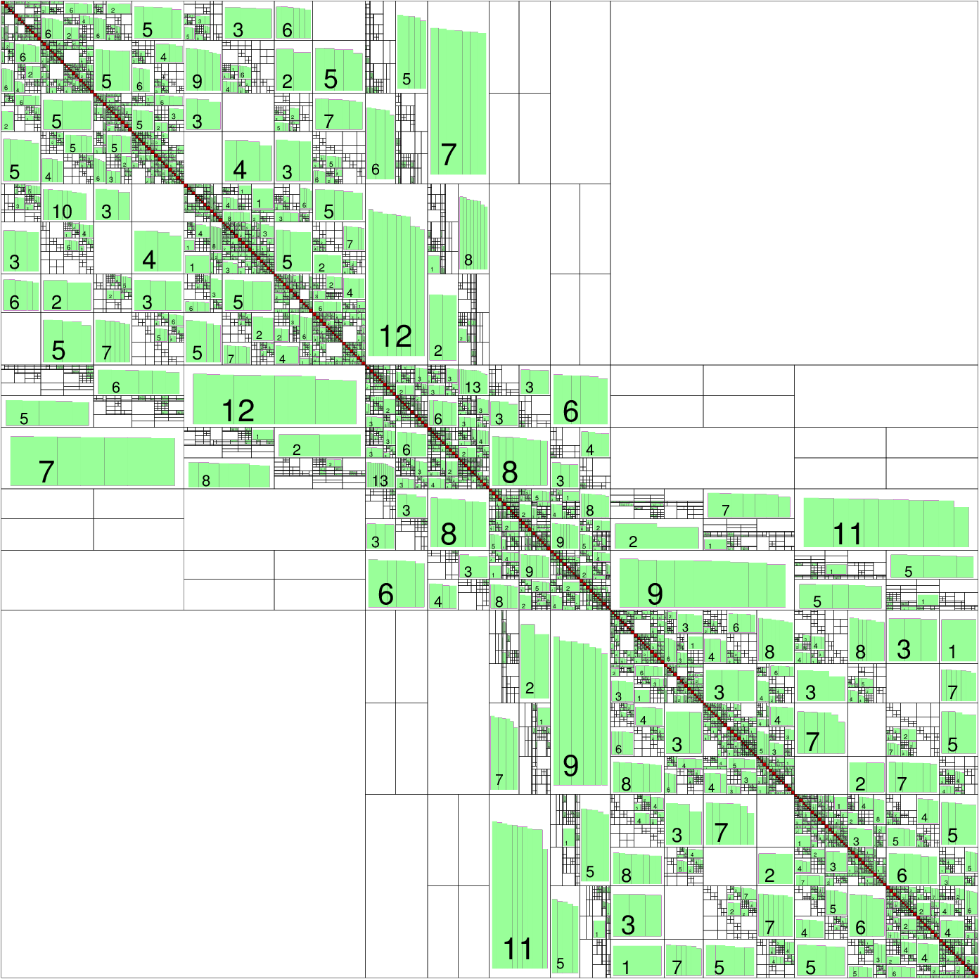
weakly admissible FEM-matrix

Figure 2. Comparison of the partition for $\eta$-admissibility and for weak admissibility. Red blocks correspond to full matrices, green blocks correspond to low-rank matrices with inscribed rank, and white blocks are zero.

4.3. Nested dissection

While the weak admissibility takes the sparsity of the finite element matrix into account only during the construction of the $\mathcal{H}$-matrix, it is also possible to incorporate the sparsity already during the construction of the cluster tree. One possibility to do so was introduced in [24] and is based on nested dissection, cf. [11, 19, 37, 45] and the references therein. We briefly review the idea of nested dissection in the context of $\mathcal{H}$-matrices as discussed in [24] and refer to [24] for more details.

The idea is to employ a recursive algorithm as follows.

1. Split degrees of freedom into three disjoint subsets $\mathcal{I}_{1}$, $\mathcal{I}_{2}$, $\mathcal{I}_{3}$ according to the following conditions.

   • $\mathcal{I}_{1}$ and $\mathcal{I}_{2}$ should have comparable sizes.

   • $\mathcal{I}_{1}$ and $\mathcal{I}_{2}$ should not interact with each other, i.e., all entries $\mathbf{A}_{i,j}$, $i\in\mathcal{I}_{1}$, $j\in\mathcal{I}_{2}$ of the finite element matrix are zero.

   • $\mathcal{I}_{3}$ is the boundary layer between $\mathcal{I}_{1}$ and $\mathcal{I}_{2}$.

2. Relabel indices in subsequent order: first $\mathcal{I}_{1}$, then $\mathcal{I}_{2}$, and then $\mathcal{I}_{3}$.

3. Proceed recursively with $\mathcal{I}_{1}$ and $\mathcal{I}_{2}$ (in the $\mathcal{H}$-matrix framework, $\mathcal{I}_{3}$ will also receive a recursive treatment).

Reordering the index sets of the finite element matrix in accordance with this procedure yields a sparsity pattern as illustrated in Figure 3. Due to the special construction, large parts of the matrix are zero and will remain zero in a subsequent LU-decomposition.

In the following, we take the approach of [24] to construct an $\mathcal{H}$-matrix which reorders the index set such that the pattern of the finite element matrix exposes a nested dissection ordering. We therefore recapitulate the construction of a cluster tree based on domain decomposition as proposed in [24]. For that purpose, the cluster algorithm distinguishes between domain clusters and interface clusters. The following algorithm is employed for the root $\{1,\ldots,N\}$ and all domain clusters.

1. Given a cluster $\sigma$ and its corresponding set of points $\{\mathbf{x}_{1},\ldots,\mathbf{x}_{\#\sigma}\}$, construct an axis-parallel bounding box $Q_{\sigma}$.

2. Cut $Q_{\sigma}$ into two pieces $Q_{1}$ and $Q_{2}$ by halving the longest edge.

3. Define three disjoint sons of $\sigma$ as follows.

   • $\sigma_{1}=\{i\colon\mathbf{x}_{i}\in Q_{1}\}$,

   • $\sigma_{2}=\{i\colon\Upsilon_{i}\cap\Upsilon_{\sigma_{1}}=\emptyset\}$,

   • $\sigma_{3}=\sigma\setminus\{\sigma_{1}\cup\sigma_{2}\}$.

4. Relabel indices of clusters in subsequent order: first $\sigma_{1}$, then $\sigma_{2}$, and then $\sigma_{3}$.

5. Treat $\sigma_{1}$ and $\sigma_{2}$ as domain clusters and $\sigma_{3}$ as interface cluster as indicated below.

Due to their special construction, the bounding boxes of interface clusters are “flat” in one coordinate direction. The cluster algorithm has therefore to be adapted to fit the asymptotic requirements of Section 3.1. Therefore, we define $\operatorname{level}_{\text{int}}(\sigma)$ as the distance of $\sigma$ to the nearest domain cluster in the cluster tree. We then employ the following cluster algorithm for the interface clusters and refer to [24] for a detailed discussion.

1. Distinguish two cases:

   • If $\operatorname{level}_{\text{int}}(\sigma)=0\mod d$: do not subdivide $\sigma$ and set $\sigma^{\prime}=\sigma$ as its only son.

   • If $\operatorname{level}_{\text{int}}(\sigma)\neq 0\mod d$: split the bounding box $Q_{\sigma}$ axis parallel in two boxes $Q_{1}$ and $Q_{2}$ such that the “flat” direction is not modified. Then define the two son clusters $\sigma_{1}=\{i\colon\mathbf{x}_{i}\in Q_{1}\}$ and $\sigma_{2}=\{i\colon\mathbf{x}_{i}\in Q_{2}\}$.

2. Apply the cluster algorithm for interface clusters to all sons.

In order to translate the sparsity of the finite element matrix into the block structure of an $\mathcal{H}$-matrix, we can combine the $\eta$-admissibility condition from (11) and the weak admissibility condition from Definition 4.1 to a nested dissection admissibility condition.

Definition 4.2.

Two clusters $\sigma$ and $\sigma^{\prime}$ are called nd-admissible if either

• $\sigma\neq\sigma^{\prime}$ are both domain clusters or

• $\sigma$ and $\sigma^{\prime}$ are $\eta$-admissible.

In fact, if $\sigma\neq\sigma^{\prime}$ are both domain clusters, we can directly say that the corresponding $\mathcal{H}$-matrix block has rank zero. Figure 3 illustrates the sparsity pattern of the finite element matrix after the permutations determined by the cluster algorithms and how large parts of the corresponding $\mathcal{H}$-matrix have rank zero.

sparse FEM-matrix

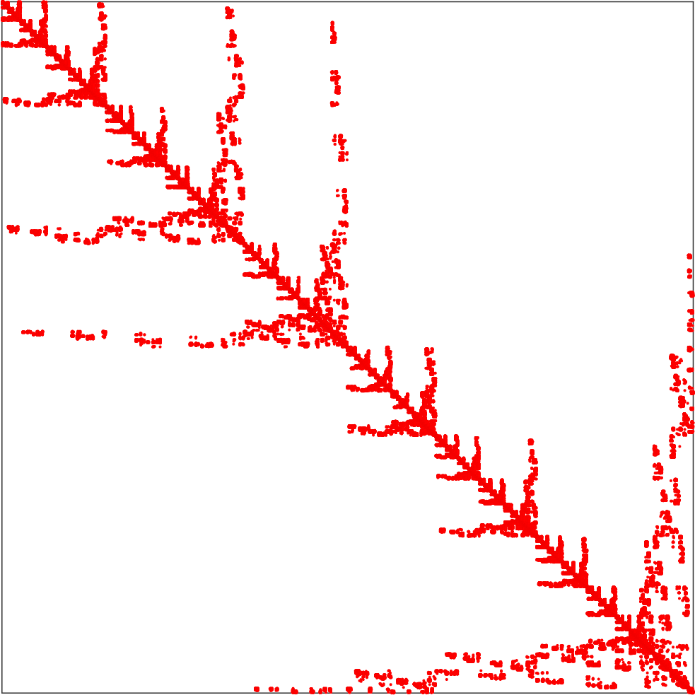
nested dissection

reordered FEM-matrix

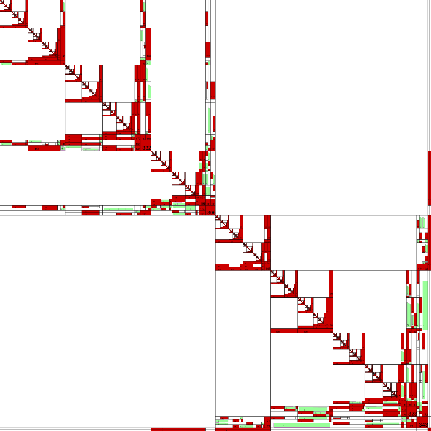
nested dissection

$\mathcal{H}$-matrix representation

Figure 3. Sparsity pattern of a 3D finite element matrix, its reordered finite element matrix according to nested dissection and its corresponding $\mathcal{H}$-matrix.

The low-rank blocks in the representation are due to some internal checks of HLib, which aim at replacing inadmissible blocks by low-rank matrices only if very few entries in the corresponding matrix block are non-zero.

The numerical experiments in the next section show that the sparse structure constructed here leads to smaller constants in the complexity of the solution algorithm.

5. Numerical results

Before we summarize the settings of the numerical experiments, we briefly recall that the algorithm of the presented method consists of the following three steps.

1. Compute the sparse finite element matrix $\mathbf{A}$ in linear and the correlation $\mathcal{H}$-matrix $\mathbf{C}_{f}$ in almost linear time.

2. Compute the approximate LU-decomposition of $\mathbf{A}$ in $\mathcal{H}$-matrix format in almost linear time.

3. Solve the matrix equation (9) with iterative refinement (13) in almost linear time for each iteration.

The numerical experiments in this article shall mainly focus on the third step and the overall behaviour of the method. We will see that only one iteration is required in the third step, which yields an almost linear overall complexity of the algorithm. To improve the computation time, we store and compute only the lower part of $\mathbf{C}_{f}$ and $\mathbf{C}_{u}$.

All the computations in the following experiments have been carried out on a single core of a computing server with two Intel(R) Xeon(R) E5-2670 CPUs with a clock rate of 2.60GHz and a main memory of 256GB. For the $\mathcal{H}$-matrix computations, we use the software package HLib, cf. [9], and for the finite element discretization the Partial Differential Equation Toolbox of Matlab which employs piecewise linear finite elements. The two libraries are coupled together in a single C-program, cf. [41], using the Matlab Engine interface. The meshes are generated by Tetgen, cf. [54], and then imported into Matlab.

5.1. Experimental setup

To obtain computational efficiency and to keep the ranks of the low-rank matrices under control, HLib imposes an upper threshold $k_{\eta}$ for the ranks in the case of an $\eta$-admissible $\mathcal{H}$-matrix and a lower threshold $n_{\min}$ for the minimal block size. For the application of the weak admissibility condition, we rely on the criterion of HLib, which considers the weak admissibility condition only if one of the index sets of the block cluster $\sigma\times\sigma^{\prime}$ has a cardinality below 1,024 and the condition

$$a_{i}^{\sigma}<\frac{a_{i}^{\sigma^{\prime}}+b_{i}^{\sigma^{\prime}}}{2}<b_{i}^{\sigma}\quad\text{or}\quad a_{i}^{\sigma^{\prime}}<\frac{a_{i}^{\sigma}+b_{i}^{\sigma}}{2}<b_{i}^{\sigma^{\prime}}$$

is satisfied for the corresponding bounding boxes $\prod_{i=1}^{3}[a_{i}^{\mu},b_{i}^{\mu}]$, $\mu=\sigma,{\sigma^{\prime}}$, in at most one coordinate direction. Otherwise, the $\eta$-admissibility is used instead. In the case of a weakly admissible matrix block, HLib imposes an upper threshold of $k_{w}=3k_{\eta}$, setting $c_{\eta\rightarrow w}=3$ in (14). For our experiments, we choose $\eta=2$, $k_{\eta}=20$, $n_{\min}=50$ and employ either a geometric cluster strategy, i.e., the binary cluster strategy from the end of Section 3.1 or the nested dissection cluster strategy as discussed in Section 4.3. The iterative refinement is stopped if the absolute error of the residual in the Frobenius norm is smaller than $10^{-6}$.

In the following examples, we want, besides other aspects, to study the influence of the weak admissibility condition and the nested dissection clustering for the partitioning of the different $\mathcal{H}$-matrices. Namely, we successively want to replace the $\eta$-admissibility by the weak admissibility for a binary and a nested dissection cluster tree as described in Table 1 in order to lower the constants hidden in the complexity of the $\mathcal{H}$-matrix arithmetic and thus to improve the computation time. For the discretization of the correlation kernel $\operatorname{Cor}_{f}$, we will always use ACA.

Case	Operator and admissibility		Cluster tree
	$\mathcal{L}$ and $\mathcal{L}^{-1}$	$\operatorname{Cor}_{f}$ and $\operatorname{Cor}_{u}$
all-$\eta$	$\eta$-admissibility	$\eta$-admissibility	binary
weak-FEM	weak admissibility	$\eta$-admissibility	binary
all-weak	weak admissibility	weak admissibility	binary
nd-$\eta$	nd-admissibility	$\eta$-admissibility	nested dissection
nd-weak	nd-admissibility	weak-admissibility	nested dissection

Table 1. The five combinations of the admissibility conditions used for the partition of the $\mathcal{H}$-matrices.

The all-$\eta$ case is the canonical case and has also been investigated in case of the boundary element method in [14]. The weak-FEM case is a first relaxation to apply the weak admissibility condition. This is justified, since the stiffness matrix $\mathbf{A}$ can exactly be represented as a weakly admissible $\mathcal{H}$-matrix and the iterative refinement only involves an approximate LU-decomposition. Hence, we expect at most an influence on the quality of the approximate LU-decomposition and thus on the number of iterations in the iterative refinement. We have therefore to investigate if possible additional iterations are compensated by the faster $\mathcal{H}$-matrix arithmetic.

The aforementioned cases have in common that they rely on the asymptotic smoothness of $\operatorname{Cor}_{f}$ and $\operatorname{Cor}_{u}$ and the $\eta$-admissibility which leads to exponential convergence of the $\mathcal{H}$-matrix approximation. In the case all-weak, we want to examine if there is some indication that the weak admissibility could possibly also be considered for the partition of the $\mathcal{H}$-matrices for $\operatorname{Cor}_{f}$ and $\operatorname{Cor}_{u}$. To that end, we approximate $\operatorname{Cor}_{f}$ with ACA relative to the $\eta$-admissibility partition and convert it on-the-fly to the partition of the weak admissibility, as proposed in [30].

While the three aforementioned cases all rely on a binary cluster tree, the cases nd-$\eta$ and nd-weak rely on a cluster tree which is constructed by nested dissection. In both cases, the finite element matrix $\mathbf{A}$ is partitioned by the nd-admissibility. For $\operatorname{Cor}_{f}$ and $\operatorname{Cor}_{u}$, we use the $\eta$-admissibility in the nd-$\eta$-case and the weak admissibility in the nd-weak-case, where we assemble the matrix for $\operatorname{Cor}_{f}$ in the same way as in the all-weak-case.

The following numerical examples are divided in two parts. In the first part, we demonstrate the convergence of the presented method by comparing it to a low-rank reference solution computed with the pivoted Cholesky decomposition, cf. [33]. In the second part, we will demonstrate that the presented method works also well in the case of correlation kernels with low Sobolev smoothness or small correlation length, where no low-rank approximations exist and sparse tensor product approximations fail to resolve the correlation length. Note that in both examples, due to the non-locality of the correlation kernels and the Green’s function, the computed system matrices are smaller than usual for the finite element method. In particular, the unknown in the system of equations (9) is a matrix with $N^{2}$ entries, whereas the corresponding mesh has only $N$ degrees of freedom. The $\mathcal{H}$-matrix compression reduces the computational complexity for the assembly and the amount of required storage from $N^{2}$ to $\mathcal{O}(kN\log N)$, whereas the complexity of the solution algorithm decreases from $\mathcal{O}(N^{3})$ to $\mathcal{O}(k^{2}N\log^{2}N)$.

5.2. Tests for the iterative solver

Due to the recompression schemes in the block matrix algorithms of the $\mathcal{H}$-matrix arithmetic, it is not directly clear if the presented solver converges. Still, it can be shown that some iterative $\mathcal{H}$-matrix schemes converge up to a certain accuracy, cf. [31]. In the following, we want to demonstrate for a specific example that our iterative scheme provides indeed convergence.

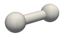
Figure 4. The dumbbell geometry and its meshed cross section with the trace of the solution correlation kernel $\operatorname{Cor}_{u}|_{\mathbf{x}=\mathbf{y}}$ for load data prescribed by the Matérn-5/2 kernel.

On the dumbbell geometry pictured in Figure 4, we consider $\mathcal{L}=-\Delta$ in (3) and the Matérn-5/2 kernel as input correlation $\operatorname{Cor}_{f}$, i.e., for $r=\|\mathbf{x}-\mathbf{y}\|_{2}$, we set

$$\operatorname{Cor}_{f}(\mathbf{x},\mathbf{y})=\bigg{(}1+\sqrt{5}\frac{r}{\ell}+\frac{5}{3}\frac{r^{2}}{\ell^{2}}\bigg{)}\exp\Big{(}-\sqrt{5}\frac{r}{\ell}\Big{)},$$

where $\ell\approx\operatorname{diam}(D)$ denotes the correlation length. The conversion of the finite element matrix to an $\mathcal{H}$-matrix for the dumbbell geometry has already been illustrated in Figure 1. Whereas, the difference between the $\eta$-admissibility and the weak admissibility is illustrated in Figure 2 and the effect of the nested dissection ordering is illustrated in Figure 3.

Level	1	2	3	4	5	Reference mesh
Mesh points	238	1,498	6,958	34,112	175,562	1,033,382
$N$	4	201	1,742	13,341	98,177	756,626
$N^{2}$	$16$	40,401	3,034,564	$1.78\cdot 10^{8}$	$9.64\cdot 10^{9}$	$5.72\cdot 10^{11}$

Table 2. Mesh points and degrees of freedom of the finite element mesh $N$ and number of entries $N^{2}$ in the solution matrix for different levels of the dumbbell geometry.

For determining a reference solution, we compute a low-rank approximation $\mathbf{C}_{f}\approx\mathbf{L}_{f}\mathbf{L}_{f}^{\intercal}$ with the pivoted Cholesky decomposition as proposed in [33]. The numerical solution $\mathbf{C}_{u}$ of (9) is then given by

$$\mathbf{C}_{u}\approx\mathbf{L}_{u}\mathbf{L}_{u}^{\intercal},$$

where $\mathbf{L}_{u}$ solves $\mathbf{A}\mathbf{L}_{u}=\mathbf{L}_{f}$. To compute the error of the $\mathcal{H}$-matrix solution, we compare the correlation and the correlation’s trace $\operatorname{Cor}_{u,N}|_{\mathbf{x}=\mathbf{y}}$ of the $\mathcal{H}$-matrix approximation with the correlation and the correlation’s trace $\operatorname{Cor}_{u,N}|_{\mathbf{x}=\mathbf{y}}$ derived from the pivoted Cholesky decomposition on a finer reference mesh. We refer to Table 2 for more details on the meshes under consideration.

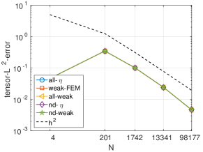
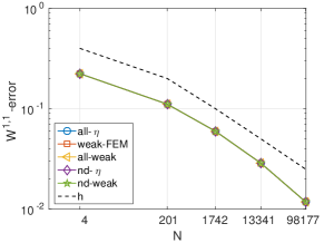
Figure 5. $L^{2}$-error of $\operatorname{Cor}_{u,N}$ (left) and $W^{1,1}$-error of $\operatorname{Cor}_{u,N}|_{\mathbf{x}=\mathbf{y}}$ (right).

While the error of the correlation itself can be measured in the $L^{2}$-norm on the tensor product domain, the appropriate norm for error measurements of it’s trace is the $W^{1,1}$-norm. Due to the Poincaré-Friedrich and the Cauchy-Schwartz inequality and

$$\big{\|}u^{2}-u_{h}^{2}\big{\|}_{W^{1,1}(D)}\lesssim\big{\|}\nabla\big{(}u^{2}-u_{h}^{2}\big{)}\big{\|}_{L^{1}(D)}\lesssim|u-u_{h}|_{H^{1}(D)}+\|u-u_{h}\|_{L^{2}(D)}\lesssim h,$$

we can expect a convergence rate in the $W^{1,1}$-norm which is proportional to the mesh size $h$. A standard tensor product argument yields a convergence rate of order $h^{2}$ in the tensor product $L^{2}$-norm. Figure 5 shows that we indeed reach these rate for all five cases of admissibility which are considered in Table 1. In fact, the observed errors coincide in the first few digits.

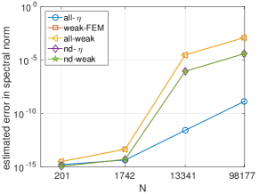
Figure 6. The deviation $\hat{\mathbf{L}}\hat{\mathbf{U}}-\mathbf{A}$ in the estimated spectral norm for fixed rank.

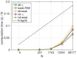
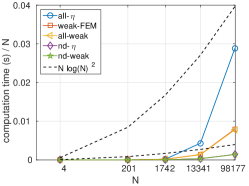
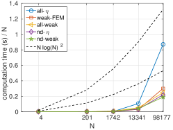
Figure 7. Computation times in seconds for the computation of the data correlation $\mathcal{H}$-matrix $\mathbf{C}_{f}$ (left), the approximate LU-decomposition of the system matrix $\mathbf{A}$ (center) and for the iterative refinement (right) on the dumbbell geometry.

We are also interested in the quality of the approximate LU-decomposition $\mathbf{A}\approx\hat{\mathbf{L}}\hat{\mathbf{U}}$. We use a built-in function of the HLib to estimate the deviation $\hat{\mathbf{L}}\hat{\mathbf{U}}-\mathbf{A}$ in the spectral norm by ten power iterations, which is a good indicator for the approximation quality of the LU-decomposition of the finite element matrix. The estimated errors are plotted in Figure 6. Note that the observed behavior is in contrast to the behavior typically observed for preconditioning, cf., e.g., [6], since we do not increase the rank with the number of unknowns. We can see that the LU-decomposition is most accurate in the all-$\eta$ case. Still, only one iteration is needed in the iterative refinement in all cases. When it comes to computation times, Figure 7 and Tables 3, 4 and 5 indicate that all cases of admissibility under consideration might yield essentially linear complexity, although the asymptotic regime seems not to be reached in the considered levels of refinement. Both, the weak admissibility condition and the nested dissection approach lead to considerable speed-ups, where the combination of these approaches, the nd-weak-case, seems to be the fastest approach. Figure 8 illustrates the required average and maximal ranks needed for the computations, whereas Figure 9 illustrates the amount of storage needed per mesh degree of freedom. For reasons of performance, the HLib allocates the worst case scenario for the ranks. Thus, in the latter case, only the different admissibilities for a single $\mathcal{H}$-matrix build from a binary and a nested dissection cluster tree have to be considered. In conclusion, the nested dissection clustering consumes less computation time and less storage for the LU-decomposition.

Level	1	2	3	4	5
all-$\eta$	0.000954	0.123520	8.07820	367.071	8,158.12
weak-FEM	0.001476	0.109641	8.12224	380.533	8,370.79
all-weak	0.001113	0.113122	8.86575	434.289	9,464.19
nd-$\eta$	0.001569	0.151018	7.54221	319.773	6,276.75
nd-weak	0.000885	0.123694	8.07407	349.585	6,711.85

Table 3. Computation times in seconds to compute the data correlation $\mathcal{H}$-matrix $\mathbf{C}_{f}$ on the dumbbell geometry.

Level	1	2	3	4	5
all-$\eta$	$2.2\cdot 10^{-5}$	0.001274	0.339432	56.2521	2,806.5
weak-FEM	$2.9\cdot 10^{-5}$	0.00143	0.315344	17.7348	743.624
all-weak	$2.2\cdot 10^{-5}$	0.001831	0.316497	18.3358	746.364
nd-$\eta$	$2.5\cdot 10^{-5}$	0.000513	0.048170	4.17870	135.778
nd-weak	$3.6\cdot 10^{-5}$	0.000588	0.050896	4.05899	132.319

Table 4. Computation times in seconds to compute the approximate LU-decomposition of the finite element matrix on the dumbbell geometry.

Level	1	2	3	4	5
all-$\eta$	$5.2\cdot 10^{-5}$	0.011115	4.68355	1,419.19	85,477.9
weak-FEM	0.000104	0.010592	2.64065	420.153	29,492.1
all-weak	$5.4\cdot 10^{-5}$	0.042098	14.5121	691.129	24,225.6
nd-$\eta$	0.000102	0.039209	5.60769	443.310	21,390.0
nd-weak	$4.4\cdot 10^{-5}$	0.061530	7.67542	544.080	18,570.5

Table 5. Computation times in seconds for the iterative refinement on the dumbbell geometry.

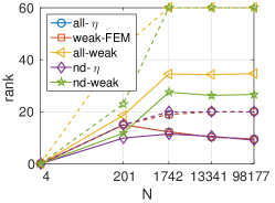
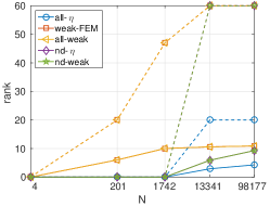
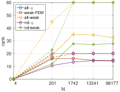
Figure 8. Required ranks for the prescribed correlation $\mathbf{C}_{f}$ (left), the LU-decomposition of $\mathbf{A}$ (middle) and the solution correlation $\mathbf{C}_{u}$ (right). The straight lines indicate the average ranks, whereas the dashed lines illustrate the maximal rank attained.

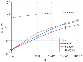
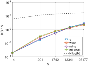
Figure 9. Allocated storage per mesh degree of freedom for different admissibility conditions. Storage for nonsymmetric (left) and symmetric matrices (right). The allocated storage is independent of the content of the matrix.

Having verified the convergence of our solver, we now want to consider different correlation lengths and different classes of smoothness.

5.3. Small correlation lengths

In the second part of the numerical experiments, we employ correlation kernels with smaller correlation lengths and lower regularity such that low-rank approximations would become prohibitively expensive and sparse tensor product approaches would fail to resolve the concentrated measure.

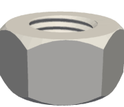
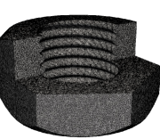
Figure 10. The screw-nut geometry (left) and its meshed cross section (right).

We consider the screw-nut geometry pictured in Figure 10 which is discretized by a mesh with 269,950 vertices, 197,480 mesh degrees of freedom, and a maximal element diameter of $h/\operatorname{diam}(D)\approx 0.0225$, yielding a matrix equation with $3.90\cdot 10^{10}$ unknowns. We choose $\mathcal{L}=-\Delta$ in (3) and either the Gaussian kernel as input correlation $\operatorname{Cor}_{f}$, i.e.,

$$\operatorname{Cor}_{f}(\mathbf{x},\mathbf{y})=\frac{1}{\ell}\exp\bigg{(}-\frac{\|\mathbf{x}-\mathbf{y}\|^{2}}{2\ell^{2}}\bigg{)},$$

or the exponential kernel, i.e.,

$$\operatorname{Cor}_{f}(\mathbf{x},\mathbf{y})=\frac{1}{\ell}\exp\bigg{(}-\frac{\|\mathbf{x}-\mathbf{y}\|}{\ell}\bigg{)}.$$

Herein, $\ell>0$ denotes the correlation length.

In the following, we want to demonstrate that the presented method is well suited for small correlation lengths $\ell$. We therefore choose the correlation lengths

$$\ell\in\bigg{\{}\frac{\operatorname{diam}(D)}{1},\frac{\operatorname{diam}(D)}{2},\frac{\operatorname{diam}(D)}{4},\frac{\operatorname{diam}(D)}{8},\frac{\operatorname{diam}(D)}{16},\frac{\operatorname{diam}(D)}{32}\bigg{\}}$$

for both, the Gaussian kernel and the exponential kernel, and compute the corresponding correlation of the solution $\operatorname{Cor}_{u}$ of (3).

In our first experiment, we use the nd-weak case, as the previous section has shown that it is more memory efficient and has superior computation times. The computation time for the assembly of the prescribed correlation is around 20,000 seconds and the computation time of the approximate LU-decomposition is around 400 seconds, whereas the computation times for the iterative refinement are contained in Table 6.

	$\ell/\operatorname{diam}(D)$	1	1/2	1/4	1/8	1/16	1/32
Exponential	nd-weak	51,656.7	53,011.0	52,876.5	51,459.2	49,838.2	51,524.6
	all-weak	77,784.5	79,101.8	79,155.3	79,155.3	76,952.6	72,256.9
Gaussian	nd-weak	47,921.8	50,644.0	50,819.5	51,753.7	—	—
	all-weak	73,405.4	74,877.0	75,165.7	68,222.8	72,259.4	75,070.4

Table 6. Computation times in seconds for the nd-weak case and for the all-weak case for the iterative refinement on the screw-nut geometry for the exponential kernel and the Gaussian kernel with different correlation lengths.

We do not tabulate the computation times for the Gaussian kernel for the correlation lengths $\ell/\operatorname{diam}(D)=1/16$ and $\ell/\operatorname{diam}(D)=1/32$ since the iterative refinement does not converge to the prescribed tolerance. In all other cases, the iterative refinement needs only one iteration.

Repeating the computations in the two problematic cases with increased $k_{\eta}$ or in the nd-$\eta$ instead of the nd-weak case does also not lead to convergence. However, repeating all computations in the all-weak case resolves the issue, as the computation times in Table 6 show. In the all-weak case, the computation time for the prescribed correlation is again around 20,000 seconds and the computation time for the approximate LU-decomposition is around 1,700 seconds. The iterative refinement needs again one iteration in all tabulated cases.

$\ell=\frac{\operatorname{diam}(D)}{1}$

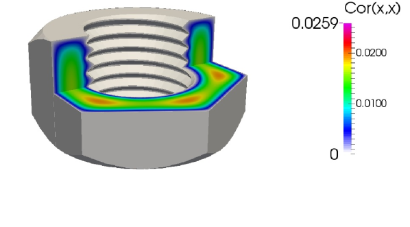
$\ell=\frac{\operatorname{diam}(D)}{2}$

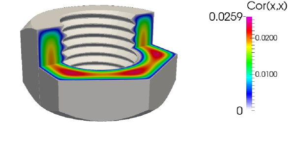
$\ell=\frac{\operatorname{diam}(D)}{4}$

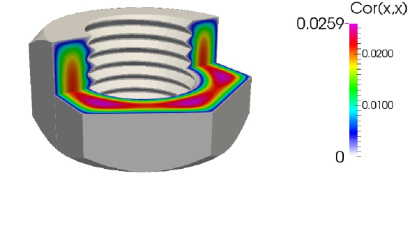
$\ell=\frac{\operatorname{diam}(D)}{8}$

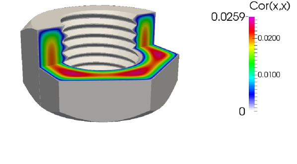
$\ell=\frac{\operatorname{diam}(D)}{16}$

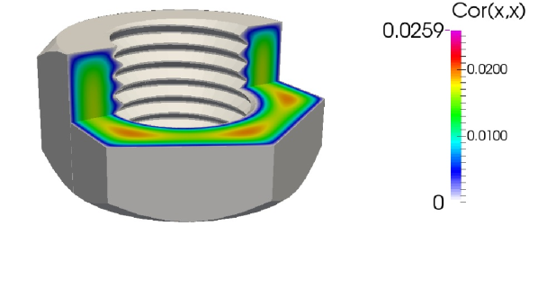
$\ell=\frac{\operatorname{diam}(D)}{32}$

Figure 11. Cross sections of the correlation of the solution through the screw-nut geometry for the exponential kernel with different correlation lengths $\ell$.

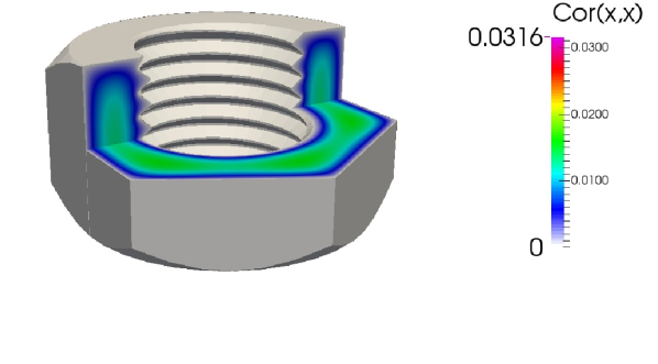
$\ell=\frac{\operatorname{diam}(D)}{1}$

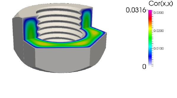
$\ell=\frac{\operatorname{diam}(D)}{2}$

$\ell=\frac{\operatorname{diam}(D)}{4}$

$\ell=\frac{\operatorname{diam}(D)}{8}$

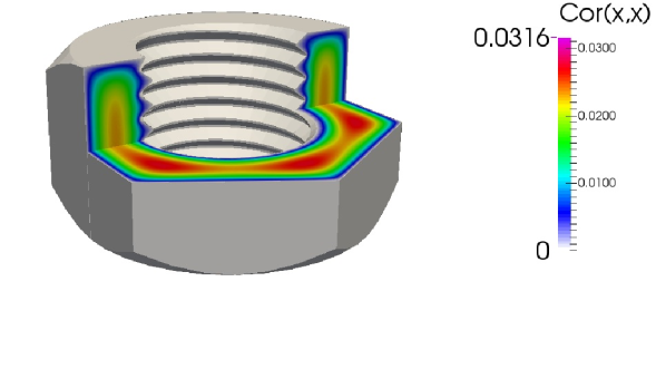
$\ell=\frac{\operatorname{diam}(D)}{16}$

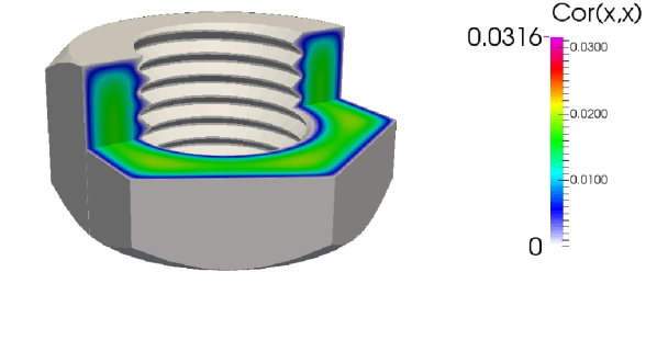
$\ell=\frac{\operatorname{diam}(D)}{32}$

Figure 12. Cross sections of the correlation of the solution through the screw-nut geometry for the Gaussian kernel with different correlation lengths $\ell$.

The cross sections found in Figure 11 illustrate the different behaviour of the correlation’s trace $\operatorname{Cor}_{u}|_{\mathbf{x}=\mathbf{y}}$ for the different correlation lengths in case of the exponential kernel. The related results for the Gaussian kernel are presented in Figure 12. It seems that there occours a mass defect in the correlation lengths $\ell/\operatorname{diam}(D)=1/16$ and $\ell/\operatorname{diam}(D)=1/32$. This could be due to the fact that the mesh size of the finite element method is not able to resolve the correlation length properly. Nevertheless, the computation times are independent of $\ell$, even if the underlying finite element method cannot resolve the correlation length. Moreover, the nested dissection clustering technique can lead to a speed-up, while the binary clustering technique seems to be more robust.

6. Conclusion

We considered the solution of strongly elliptic partial differential equations with random load by means of the finite element method. Approximating the full tensor approach by means of $\mathcal{H}$-matrices, we employed the $\mathcal{H}$-matrix technique to efficiently discretize the non-local correlation kernel of the data and approximate the LU-decomposition of the finite element stiffness matrix. The corresponding $\mathcal{H}$-matrix equation has then been efficiently solved in essentially linear complexity by the $\mathcal{H}$-matrix arithmetic.

Compared to sparse tensor product or low-rank approximations, the proposed method does not suffer in case of shortly correlated data from large constants in the complexity estimates or the lack of resolution of the roughness. This has been shown by numerical experiments on a non-trivial three-dimensional geometry. Indeed, neither the computation times nor the storage requirements do increase for correlation kernels with short correlation length. It was moreover demonstrated that the use of the weak admissibility condition for the partition of the $\mathcal{H}$-matrix improves the constants in the computational complexity without having a significant impact to the solution accuracy. The use of a nested dissection clustering strategy can additionally lead to a speed-up of the computations and save storage, whereas the binary clustering strategy seems to be the more robust approach.

References

- [1] I. Babuška, F. Nobile, and R. Tempone, A stochastic collocation method for elliptic partial differential equations with random input data, SIAM Journal on Numerical Analysis 45 (2007), no. 3, 1005–1034.
- [2] I. Babuška, R. Tempone, and G. Zouraris, Galerkin finite element approximations of stochastic elliptic partial differential equations, SIAM Journal on Numerical Analysis 42 (2004), no. 2, 800–825.
- [3] M. Bebendorf, Approximation of boundary element matrices, Numerische Mathematik 86 (2000), no. 4, 565–589.
- [4] by same author, Efficient inversion of the Galerkin matrix of general second-order elliptic operators with nonsmooth coefficients, Mathematics of Computation 74 (2005), no. 251, 1179–1199.
- [5] by same author, Why finite element discretizations can be factored by triangular hierarchical matrices, SIAM Journal on Numerical Analysis 45 (2007), no. 4, 1472–1494.
- [6] by same author, Hierarchical matrices, Lecture Notes in Computational Science and Engineering, vol. 63, Springer Berlin Heidelberg, 2008.
- [7] M. Bebendorf and W. Hackbusch, Existence of -matrix approximants to the inverse FE-matrix of elliptic operators with -coefficients, Numerische Mathematik 95 (2003), no. 1, 1–28.
- [8] S. Börm, Efficient Numerical Methods for Non-local Operators, EMS Tracts in Mathematics, vol. 14, European Mathematical Society (EMS), Zürich, 2010. MR 2767920 (2012i:65001)
- [9] S. Börm, L. Grasedyck, and W. Hackbusch, Hierarchical matrices, Tech. Report 21, Max Planck Institute for Mathematics in the Sciences, 2003.
- [10] L. Boutet de Monvel and P. Krée, Pseudo-differential operators and Gevrey classes, Annales de l’Institut Fourier (Grenoble) 17 (1967), no. fasc. 1, 295–323. MR 0226170 (37 #1760)
- [11] I. Brainman and S. Toledo, Nested-dissection orderings for sparse LU with partial pivoting, SIAM Journal on Matrix Analysis and Applications 23 (2002), no. 4, 998–1012.
- [12] R. Caflisch, Monte Carlo and quasi-Monte Carlo methods, Acta Numerica 7 (1998), 1–49.
- [13] M. Deb, I. Babuška, and J. Oden, Solution of stochastic partial differential equations using Galerkin finite element techniques, Computer Methods in Applied Mechanics and Engineering 190 (2001), no. 48, 6359–6372. MR 1870425 (2003g:65009)
- [14] J. Dölz, H. Harbrecht, and M. Peters, -matrix accelerated second moment analysis for potentials with rough correlation, Journal of Scientific Computing 65 (2015), no. 1, 387–410.
- [15] J. Dölz, H. Harbrecht, and Ch. Schwab, Covariance regularity and -matrix approximation for rough random fields, Numerische Mathematik 135 (2017), no. 4, 1045–1071.
- [16] M. Faustmann, Approximation inverser Finite Elemente- und Randelementematrizen mittels hierarchischer matrizen, PHD Thesis, Technische Universität Wien, 2015.
- [17] M. Faustmann, J. M. Melenk, and D. Praetorius, -matrix approximability of the inverses of FEM matrices, Numerische Mathematik 131 (2015), no. 4, 615–642.
- [18] P. Frauenfelder, C. Schwab, and R.A. Todor, Finite elements for elliptic problems with stochastic coefficients, Computer Methods in Applied Mechanics and Engineering 194 (2005), no. 2-5, 205–228.
- [19] Alan George, Nested dissection of a regular finite element mesh, SIAM Journal on Numerical Analysis 10 (1973), no. 2, 345–363.
- [20] R. Ghanem and P. Spanos, Stochastic Finite Elements: A Spectral Approach, Springer, New York, 1991.
- [21] D. Gilbarg and N.S. Trudinger, Elliptic partial differential equations of second order, Springer, Berlin-Heidelberg, 1977.
- [22] G.H. Golub and C.F. Van Loan, Matrix Computations, 4th ed., Johns Hopkins University Press, Baltimore, 2012.
- [23] L. Grasedyck and W. Hackbusch, Construction and arithmetics of -matrices, Computing 70 (2003), no. 4, 295–334.
- [24] L. Grasedyck, R. Kriemann, and S. Le Borne, Domain decomposition based -LU preconditioning, Numerische Mathematik 112 (2009), no. 4, 565–600.
- [25] L. Greengard and V. Rokhlin, A fast algorithm for particle simulations, Journal of Computational Physics 73 (1987), no. 2, 325–348.
- [26] M. Griebel and H. Harbrecht, Approximation of bi-variate functions: singular value decomposition versus sparse grids, IMA Journal of Numerical Analysis 34 (2014), no. 1, 28–54.
- [27] W. Hackbusch, A sparse matrix arithmetic based on -matrices part I: Introduction to -matrices, Computing 62 (1999), no. 2, 89–108.
- [28] by same author, Hierarchical Matrices: Algorithms and Analysis, Springer, Heidelberg, 2015.
- [29] W. Hackbusch and B.N. Khoromskij, A sparse -matrix arithmetic. General complexity estimates, Journal of Computational and Applied Mathematics 125 (2000), no. 1–2, 479–501.
- [30] W. Hackbusch, B.N. Khoromskij, and R. Kriemann, Hierarchical matrices based on a weak admissibility criterion, Computing 73 (2004), no. 3, 207–243.
- [31] W. Hackbusch, B.N. Khoromskij, and E.E. Tyrtyshnikov, Approximate iterations for structured matrices, Numerische Mathematik 109 (2008), no. 3, 365–383.
- [32] H. Harbrecht, A finite element method for elliptic problems with stochastic input data, Applied Numerical Mathematics 60 (2010), no. 3, 227–244.
- [33] H. Harbrecht, M. Peters, and R. Schneider, On the low-rank approximation by the pivoted Cholesky decomposition, Applied Numerical Mathematics 62 (2012), 28–440.
- [34] H. Harbrecht, M. Peters, and M. Siebenmorgen, Combination technique based -th moment analysis of elliptic problems with random diffusion, Journal of Computational Physics 252 (2013), 128–141.
- [35] H. Harbrecht, R. Schneider, and C. Schwab, Multilevel frames for sparse tensor product spaces, Numerische Mathematik 110 (2008), no. 2, 199–220.
- [36] by same author, Sparse second moment analysis for elliptic problems in stochastic domains, Numerische Mathematik 109 (2008), no. 3, 385–414.
- [37] B. Hendrickson and E. Rothberg, Improving the run time and quality of nested dissection ordering, SIAM Journal on Scientific Computing 20 (1998), no. 2, 468–489.
- [38] L. Hörmander, The Analysis of Linear Partial Differential Operators. I, Classics in Mathematics, Springer, Berlin, 2003, Distribution theory and Fourier analysis, Reprint of the second (1990) edition. MR 1996773
- [39] by same author, The Analysis of Linear Partial Differential Operators. III, Classics in Mathematics, Springer, Berlin, 2007, Pseudo-differential operators, Reprint of the 1994 edition.
- [40] G.C. Hsiao and W.L. Wendland, Boundary Integral Equations, Applied Mathematical Sciences, vol. 164, Springer, Berlin, 2008. MR 2441884 (2009i:45001)
- [41] B.W. Kernighan and D.M. Ritchie, The C Programming Language, Prentice-Hall, Upper Saddle River, NJ, 1988.
- [42] B.N. Khoromskij and C. Schwab, Tensor-structured Galerkin approximation of parametric and stochastic elliptic PDEs, SIAM Journal on Scientific Computing 33 (2011), no. 1, 364–385.
- [43] R. Kriemann, Parallel-matrix arithmetics on shared memory systems, Computing 74 (2005), no. 3, 273–297.
- [44] by same author, -LU factorization on many-core systems, Computing and Visualization in Science 16 (2013), no. 3, 105–117.
- [45] R. J. Lipton, D. J. Rose, and R. E. Tarjan, Generalized nested dissection, SIAM Journal on Numerical Analysis 16 (1979), no. 2, 346–358.
- [46] B. Matérn, Spatial variation, Springer Lecture Notes in Statistics, Springer, New York, 1986.
- [47] H. Matthies and A. Keese, Galerkin methods for linear and nonlinear elliptic stochastic partial differential equations, Computer Methods in Applied Mechanics and Engineering 194 (2005), no. 12-16, 1295–1331.
- [48] C.B. Moler, Iterative refinement in floating point, Journal of the ACM 14 (1967), no. 2, 316–321.
- [49] F. Nobile, R. Tempone, and C.G. Webster, An anisotropic sparse grid stochastic collocation method for partial differential equations with random input data, SIAM Journal on Numerical Analysis 46 (2008), no. 5, 2411–2442. MR 2421041 (2009c:65331)
- [50] C.E. Rasmussen and C.K.I. Williams, Gaussian processes for machine learning (adaptive computation and machine learning), The MIT Press, Cambridge, 2005.
- [51] Y. Saad, Iterative methods for sparse linear systems, second ed., Society for Industrial and Applied Mathematics, 2003.
- [52] C. Schwab and R.A. Todor, Sparse finite elements for elliptic problems with stochastic loading, Numerische Mathematik 95 (2003), no. 4, 707–734.
- [53] by same author, Karhunen-Loève approximation of random fields by generalized fast multipole methods, Journal of Computational Physics 217 (2006), 100–122.
- [54] H. Si, Tetgen, a delaunay-based quality tetrahedral mesh generator, ACM Trans. Math. Softw. 41 (2015), no. 2, 11:1–11:36.
- [55] M.E. Taylor, Pseudodifferential Operators, Princeton Mathematical Series, vol. 34, Princeton University Press, Princeton, NJ, 1981. MR 618463 (82i:35172)
- [56] E. Tyrtyshnikov, Mosaic sceleton approximation, Calcolo 33 (1996), 47–57.
- [57] T. von Petersdorff and C. Schwab, Sparse finite element methods for operator equations with stochastic data, Applications of Mathematics 51 (2006), no. 2, 145–180.
- [58] J.H. Wilkinson, Rounding errors in algebraic processes, Prentice Hall, Englewood Cliffs, NJ, 1963.
- [59] D. Xiu and D.M. Tartakovsky, Numerical methods for differential equations in random domains, SIAM Journal on Scientific Computing 28 (2006), no. 3, 1167–1185.