1 Abstract

To account for the ability of living organisms to reason with uncertain and incomplete information, it has been recently proposed that the brain is a probabilistic inference machine, evaluating subjective probabilistic models over cognitively relevant variables. A number of such Bayesian models have been shown to account efficiently for perceptive and behavioral tasks. However, little is known about the way these subjective probabilities are represented and processed in the brain. Several theoretical proposals have been made, from large populations of neurons to specialized cortical microcircuits or individual neurons as potential substrates for such subjective probabilistic inferences. In contrast, we propose in this paper that at a subcellular level, biochemical cascades of cell signaling can perform the necessary probabilistic computations. Specifically, we propose that macromolecular assemblies (receptors, ionic channels, and allosteric enzymes) coupled through several diffusible messengers (G-proteins, cytoplasmic calcium, cyclic nucleotides and other second messengers, membrane potentials, and neurotransmitters) are the biochemical substrates for subjective probability evaluation and updating. On one hand, the messengers’ concentrations play the role of parameters encoding probability distributions; on the other hand, allosteric conformational changes compute the probabilistic inferences. The method used to support this thesis is to prove that both subjective cognitive probabilistic models and the descriptive coupled Markov chains used to model these biochemical cascades are performing equivalent computations. On one hand, we demonstrate that Bayesian inference on subjective models is equivalent to the computation of some rational function with nonnegative coefficient (RFNC), and, on the other hand, that biochemical cascades may also be seen as computing RFNCs. This suggests that the ability to perform probabilistic reasoning is a very fundamental characteristic of biological systems, from unicellular organisms to the most complex brains.

2 Author Summary

Living organisms survive and multiply even though they have uncertain and incomplete information about their environment and imperfect models to predict the consequences of their actions. Bayesian models have been proposed to face this challenge. Indeed, Bayesian inference is a way to do optimal reasoning when only uncertain and incomplete information is available. Various perceptive, sensory-motor, and cognitive functions have been successfully modeled this way. However, the biological mechanisms allowing animals and humans to represent and to compute probability distributions are not known. It has been proposed that neurons and assemblies of neurons could be the appropriate scale to search for clues to probabilistic reasoning. In contrast, in this paper, we propose that interacting populations of macromolecules and diffusible messengers can perform probabilistic computation. This suggests that probabilistic reasoning, based on cellular signaling pathways, is a fundamental skill of living organisms available to the simplest unicellular organisms as well as the most complex brains.

3 Introduction

The information available to living organisms about their environment is uncertain, not only because biological sensors are imperfect, but more importantly because sensors inevitably provide an incomplete, partial description of the environment. Moreover, timing is a crucial constraint for biological systems. During a fight-or-flight dilemma, animals must quickly decide to fight or flee, and they can never be sure of the good or bad consequences of their decision. Incompleteness is therefore a key notion for an autonomous agent facing the complexity of the world. There is now growing evidence that probabilistic reasoning is a rigorous and efficient way to represent partial or incomplete knowledge and to answer questions optimally that have no uniquely defined solution [1].

Perception is a well-known example of ill-posed problems, because an indefinite number of object characteristics can theoretically give rise to the same set of sensory data. For instance, an indefinite number of objects with various shapes, sizes and movements can induce exactly the same retinal projection. A number of studies have shown that Bayesian models can accurately account for various aspects of perception [2, 3, 4, 5, 6, 7] and sensory-motor integration [8, 9, 10, 11].

Nonprobabilistic models assume that the brain computes internal estimates of relevant state variables such as motion, object distance, and color. Each variable is supposed to have a unique estimate, on which no evaluation of uncertainty is performed. In contrast, Bayesian models assume that the brain evaluates the probability corresponding to each possible value of the relevant variables. Probability computation results from straightforward application of the Bayes (i.e., multiplicative) and marginalization (i.e., additive) rules, which can been seen as a generalization of logical inference to probability distributions [12, 13]. Following Pearl [14] and Jaynes [1], we define probabilistic reasoning as the ability to perform inference within a probabilistic knowledge base. In the following, we will call a subjective Bayesian model the specification of the variables of interest, their conditional dependencies, the parametric forms, and the way probability distributions can be inferred.

Acknowledging the efficiency of probabilistic reasoning in accounting for a large variety of perceptive reports or motor behaviors, one of the main scientific challenges is to explicitly demonstrate that the brain, and more generally biological systems, can effectively perform probabilistic computation. The problem is to show possible correspondences between subjective Bayesian models and descriptive models of biological systems and signal processing.

Most existing studies proposed assemblies of neuronal cells or single neurons as the appropriate level of analysis to explain how a brain could perform probabilistic inference. Several authors have proposed that the firing rate of a group of cells within a given temporal window [15, 16, 17] could represent probability distributions over state variables. The mean firing rate might be well approximated by a graded value, to which a subjective probabilistic meaning can be attributed: for instance, the probability that a given proposal over a state variable is true, or its log-likelihood ratio. Other approaches are based on the Poisson-like variability of spike trains [18] or kernel convolution for encoding/decoding spike trains [19].

In contrast, we consider the molecular scale as an adequate framework to solve this matching problem between subjective Bayesian models and descriptive biological ones.

Populations of macromolecules in their various conformational states and diffusible messenger concentrations are assumed to be the substates used at subcellular level to represent and to compute probability distributions. Our proposal is that the biochemical processes involved in cell signaling can perform the elementary computations needed for subjective probabilistic reasoning, and that this biochemical computation is used extensively by the brain as an elementary component: a Bayesian “nanogate.” Specifically, we propose that macromolecular assemblies (receptors, ionic channels, and allosteric enzymes) coupled through several diffusible messengers (G-proteins, cytoplasmic calcium, cyclic nucleotides and other second messengers, membrane potentials, and neurotransmitters) are the biochemical substrates for subjective probability evaluation and updating. On the one hand, messenger concentrations play the role of parameters encoding probability distributions, on the other hand, allosteric conformational changes compute the probabilistic inferences. Diffusible messenger concentrations, including electric charge density, control the probability of conformational changes, which are in turn responsible for inflow and outflow rates of messengers and are then controlling their kinetics.

We started exploring these ideas in [20], where the kinetics of a rhodopsin channel were shown to converge to a posterior distribution of states in a hidden Markov model, the hidden state representing the presence or absence of light. A similar kinetic scheme derived from Bayesian formulation of receptor activations was compared with other common signaling schemes in [21] to emphasize its optimality. Rather than considering a binary (ON or OFF) hidden state, multiple activated states were considered in [22] (like self and nonself in the immune system) and they discussed how Koshland–Goldbeter could solve this decision problem. Napp and Adams proposed in a recent paper [23] a procedure to compile a probabilistic graphical model into a chemical reaction network.

4 Results

Subjective probabilistic models (often called Bayesian models) include variables describing states of the world highly relevant for the organism, such as the presence of food or predators. The values taken by these variables cannot be known with certainty by the organism. However, according to the Bayesian approach, the organism can evaluate the probability distribution over these variables on the basis of specific observations, such as the detection of light or the detection of an odorant molecule.

Subjective probabilistic reasoning is the process by which the probabilities of relevant variables are computed from a set of observations and a set of priors and conditional dependencies between variables [13].

Descriptive biochemical models, reduce biochemical signaling mechanisms to two sets of interacting substrates: (i) macromolecular assemblies (such as receptors, ionic channels, or activatable enzymes), which have a nearly fixed spatial distribution (in the time scale we considered here), but a variable conformational state distribution; and (ii) diffusible messengers (such as G-protein $\alpha$-subunits, cyclic nucleotides, cytoplasmic calcium, and membrane potentials) that have a fixed conformational state, but a variable spatial distribution.

The messengers, when they bind to their specific receptor sites on macromolecules, induce conformational changes. The macromolecules, when they are in active states, release or remove messengers, thus changing the messengers’ spatial distribution. Continuous thermal agitation induces random events such as macromolecule allosteric transitions, messenger diffusion, and molecular collisions. Therefore, biochemical interactions can be described as a set of strongly coupled causal Markov chains, with random variables specifying internal states such as conformational states and concentrations.

The main result of this paper is a formal demonstration that concentrations of messengers in biochemical systems can represent subjective probability distributions and that conformational changes of macromolecules can perform the fundamental operations required by Bayesian inference.

To reach this goal we demonstrate, on one hand, that Bayesian inference on subjective models is equivalent to the computation of some rational function with nonnegative coefficient (RFNC) of inputs related to sensory data, and, on the other hand, that biochemical cascades may also be seen as computing RFNCs of inputs related to the concentration of primary messengers.

4.1 A basic example

The simplest subjective model has only one binary variable $S\in\{0,\,1\}$ and a single observation $K\in\mathbb{K}$. The structure of the model consists of a prior on $S$, $P(S)$, and a likelihood of the observation $K$ knowing $S$, $P(K|S)$:

$$P(S,K)=P(S)P(K|S)$$ (1)

The prior on $S$ is completely specified by the odds:

$$\frac{P([S=1])}{P([S=0])}=a$$ (2)

It is straightforward to see that $P([S=0])=1/(1+a)$ and $P([S=1])=a/(1+a)$.

The likelihood function $P(K\,|\,S)$ allows us to define a mapping $g$ from $\mathbb{K}$ to $\mathbb{R}^{+}$such that:

$$g(k)=\frac{P([K=k]\,|\,[S=1])}{P([K=k]\,|\,[S=0])}$$ (3)

For a given observation $k$, we apply this function to find the input number $x=g(k)$, from which we can compute the corresponding posterior odds:

$$y=\frac{P([S=1]\,|\,k)}{P([S=0]\,|\,k)}=ax$$ (4)

Obviously, this single nonnegative number $y$ completely specifies the posterior distribution with $P([S=0]\,|\,k)=1/(1+y)$ and $P([S=1]\,|\,k)=y/(1+y)$.

This extremely basic subjective model illustrates the two main operations required by probabilistic inference: once an observation $k$ is known, it is first transformed into a nonnegative number $x$ that we call the input (we will later show that in the general case the input is a multidimensional vector of nonnegative numbers). The input is then processed by an RFNC, reduced in this basic model to a multiplication by a constant. The output is again a nonnegative number (in the general case, a multidimensional vector of nonnegative numbers), which specifies the posterior distribution.

We will now show how these two successive operations can be implemented by a biochemical system (see Figure 1). We first consider a population of macromolecular receptors sensitive to some external stimulus. Depending on the type of receptor, the stimulus could be, for instance, a flow of photons, a mechanical strength, or the presence of nutrient in the environment. This stimulus is what the cell observes from its current environment, and its actual particular value can be denoted as $k$. This stimulus induces a conformational change, and thus the proportion of active receptors. The activity of these receptors results in the release of a primary messenger $X$ within the cell. We call $x=[X]$ the concentration of the primary messenger resulting from the stimulus $k$. The population of receptors plays exactly the role of the mapping $g$ in the subjective model. Although $k$ is not represented per se in the biochemical system, the output of the population of receptors, i.e., the primary messenger concentration $x$, represents what really matters for the inference, the likelihood ratio $g(k)$.

We next consider a second population of macromolecules $M$, each with a single receptor site, specific for the primary messenger $X$. These macromolecules could be in one of two conformations: in the first, the receptor site is free ($M=0$) and in the other the receptor binds a messenger ($M=1$). Within a small time interval $\Delta t$, the transition probability from $M=1$ to $M=0$ is a constant $\alpha$. The transition from $M=0$ to $M=1$ requires the presence of one messenger molecule in the vicinity of the receptor site; its probability is therefore proportional to the current messenger concentration $x$:

$$\begin{cases}\,\,P_{1\rightarrow 0}=P(M^{t+\Delta t}=0\,|\,M^{t}=1,\,x)=\alpha\\ \,\,P_{0\rightarrow 1}=P(M^{t+\Delta t}=1\,|\,M^{t}=0,\,x)=\beta x\end{cases}$$ (5)

Each macromolecule in the $M$ population switches randomly between state 0 and state 1 according to the transition probabilities defined above. After a while, the probability of finding the macromolecule in a given state converges to the equilibrium, or steady-state, distribution. In this case, the equilibrium distribution ($P^{*}$) follows the detailed balance equation:

$$P^{*}_{1}.P_{1\rightarrow 0}=P^{*}_{0}.P_{0\rightarrow 1}$$ (6)

and the resulting equilibrium distribution is:

$$\begin{cases}\,\,P^{*}_{0}=\alpha/(\alpha+\beta x)\\ \,\,P^{*}_{1}=\beta x/(\alpha+\beta x)\end{cases}$$ (7)

When in state 1, that is, when the primary messenger is fixed, the macromolecules release a second messenger $Y$ (concentration $y=[Y]$) at a constant rate $a_{P}$. When in state 0, that is, when the receptor site is free, the macromolecules remove the second messenger at a rate proportional to its concentration $a_{R}\times y$, so that at equilibrium we have:

$$a_{P}\times\frac{\beta x}{\alpha+\beta x}=a_{R}\times\frac{\alpha}{\alpha+\beta x}\times y$$ (8)

Finally, the resulting second messenger concentration is simply proportional to the primary messenger concentration:

$$y=\frac{a_{P}}{a_{R}}\times\frac{\beta x}{\alpha}$$ (9)

This basic example illustrates the kind of equivalence scheme that can be drawn between the subjective and descriptive models. The macromolecular receptors transform a stimulus $k$ into a likelihood ratio represented by the concentration of primary messengers, while the remainder of the biochemical chain computes a posterior ratio represented by the concentration of second messengers. Obviously, this basic model is quite elementary (see a simulation with realistic values in Figure 1). In the next two sections, we will show that the equivalence scheme is much more general.

4.2 Bayesian models and RFNCs

In this paper, we consider only subjective models where unknown variables are discrete, i.e., they have a finite, though eventually huge, number of possible values. The unknown variables can be divided into a set of relevant, or searched variables, denoted $S$ (of size $n_{S}$) and a set, eventually empty, of intermediate, or free variables, denoted $F$ (of size $n_{F}$). We do not make any restriction on the nature, discrete or not, of the set of observations $K$. Based on these assumptions, the structure of the general subjective model we consider is:

$$P(S,\,F,\,K)=P(S,\,F)\times P(K\,|\,S,\,F)$$ (10)

The right side of this equation is the product of a prior distribution $P(S,\,F)$ and a likelihood $P(K\,|\,S,\,F)$. For the organism, the problem is to compute the posterior distribution over the relevant variable $S$ knowing a given set of observations $k$ (by convention, we will use small caps for variables with known values):

$$P(S\,|\,k)=\frac{\sum_{F}\,P(S,\,F)\times P(k\,|\,S,\,F)}{\sum_{S}\sum_{F}\,P(S,\,F)\times P(k\,|\,S,\,F)}$$ (11)

The denominator on the right side of the equation is a normalization constant, which could be hard to compute if the state spaces ($S$ and $F)$ are very large. Instead, the posterior distribution is completely determined by a finite set of probability ratios:

$$\frac{P([S=s]\,|\,k)}{P([S=0]\,|\,k)}=\frac{\sum_{F}\,P([S=s],\,F)\times P(k\,|\,[S=s],\,F)}{\sum_{F}\,P([S=0],\,F)\times P(k\,|\,[S=0],\,F)}$$ (12)

where the particular state $[S=0]$ is used as a reference, or default state. One can also choose a reference value for the free variables. Providing that the prior $P([S=0],\,[F=0])$ and the likelihood $P(k\,|\,[S=0],\,[F=0])$ for the chosen reference values are not null, the posterior ratios reduce to:

$$\frac{P([S=s]\,|\,k)}{P([S=0]\,|\,k)}=\frac{\sum_{f}\,\frac{P([S=s],\,[F=f])}{P([S=0]\,[F=0])}.\frac{P(k\,|\,[S=s],\,[F=f])}{P(k\,|\,[S=0]\,[F=0])}}{\sum_{f}\,\frac{P([S=0],\,[F=f])}{P([S=0],\,[F=0])}.\frac{P(k\,|\,[S=0],\,[F=f])}{P(k\,|\,[S=0],\,[F=0])}}$$ (13)

4.2.1 From Bayesian models to RFNCs

Once a given observation $k$ is available, it can be first transformed into an input vector $x=g(k)$ of dimension $n_{SF}=n_{S}n_{F}$ with the following mapping:

$$\forall s\in\{0,...,\,n_{S}-1),\,\forall f\in\{0,...,\,n_{F}-1):\,x_{s,f}=\frac{P(k\,|\,[S=s]\,[F=f])}{P(k\,|\,[S=0]\,[F=0])}$$ (14)

Obviously, we have $x_{0,0}=1$ and all other components are nonnegative numbers.

Similarly, the prior $P(S,\,F)$ is completely specified by a vector of nonnegative constants $a$ such that:

$$\forall s\in\{0,...,\,n_{S}-1),\,\forall f\in\{0,...,\,n_{F}-1):\,a_{s,f}=\frac{P([S=s]\,[F=f])}{P([S=0]\,[F=0])}$$ (15)

Finally, the posterior $P(S\,|\,k)$ is completely specified by a vector of dimension $n_{S}$:

$$\forall s\in\{0,...,\,n_{S}-1):\,y_{s}=\frac{P([S=s]\,|\,k)}{P([S=0]\,|\,k)}$$ (16)

Equation (13) can be restated as:

$$\forall s:\,y_{s}=\frac{\sum_{f}\,a_{s,f}\times x_{s,f}}{\sum_{f}\,a_{0,f}\times x_{0,f}}$$ (17)

Obviously, we have $y_{0}=1$ and all other components are rational functions with nonnegative coefficients of the components of the input vector.

This demonstrates that the exact inference in the Bayesian model is equivalent to the application of a finite set of RFNCs to an observation-dependent vector of nonnegative numbers.

4.2.2 From RFNC to Bayesian models

Reciprocally, we will now show that from any finite set of RFNCs, one can build at least one subjective probabilistic model such that the posterior probability ratios can be computed with these RFNCs.

Let us first prove this result for a single RFNC $h$. Clearly, in this case, the search variable $S$ is a binary random variable, and the problem is to specify the subjective model such that the posterior odds is equal to $h(x)$ where $x$ is an input vector depending on the set of observations or known variables $k$.

We define the complexity of an RFNC as the number of operations (addition, multiplication, and division) required to compute the image $h(x)$ from the components of the input vector.

If $complexity(h)=0$, $h(x)$ is either a constant or one component of the input vector. There are obvious Bayesian models associated with both cases, as shown in the basic model section.

If $complexity(h)\geq 1$, then it is possible to decompose $h$ into a combination of two simpler, (i.e., lower-complexity) RFNCs $h_{1}$ and $h_{2}$ with either $h(x)=h_{1}(x)+h_{2}(x)$, $h(x)=h_{1}(x).h_{2}(x)$, or $h(x)=h_{1}(x)/h_{2}(x)$.

Suppose that we can associate $h_{1}$ with a probabilistic model $P(S_{1},\,F_{1},\,K)$, where the searched variable $S_{1}$ is binary, such that:

$$\frac{P([S_{1}=1]\,|\,k)}{P([S_{1}=0]\,|\,k)}=h_{1}(x)$$ (18)

Similarly, we suppose that we can associate $h_{2}$ with another probabilistic model $P(S_{2},\,F_{2},\,K)$ where $S_{2}$ is binary such that the posterior ratio is equal to $h_{2}(x)$.

We may assemble these two models using a generative metamodel defined by:

$$\begin{array}[]{ll}&P(S,\,S_{1},\,S_{2},\,F_{1},\,F_{2},\,K,\,K_{1},\,K_{2},\,\Lambda,\,\Gamma)\\ =&P(S)P(S_{1},\,F_{1},\,K_{1})P(S_{2},\,F_{2},\,K_{2})P(\Lambda\,|\,S,\,S_{1},\,S_{2})P(\Gamma\,|\,K,\,K_{1},\,K_{2})\end{array}$$ (19)

This metamodel uses two binary variables $\Lambda$ and $\Gamma$, which are called coherence variables (see Chapter 8 in [13]) and define how the two submodels are combined.

The distribution $P(\Gamma\,|\,K,\,K_{1},\,K_{2})$ is defined as a Dirac distribution, which means that the same set of observations $K$ is shared by both submodels:

$$P([\Gamma=1]\,|\,K,\,K_{1},\,K_{2})=1_{K=K_{1}=K_{2}}$$ (20)

The distribution $P(\Lambda\,|\,S,\,S_{1},\,S_{2})$ is defined as follows:

$$P([\Lambda=1]\,|\,[S=i],\,[S_{1}=j],\,[S_{2}=k])=q_{i,j,k}$$ (21)

where the coefficients $q_{i,j,k}$ define how $S$ is related to $S_{1}$ and $S_{2}$.

We may now consider the model specified by:

$$P(S,\,S_{1},\,S_{2},\,F_{1},\,F_{2},\,K,\,K_{1},\,K_{2}|\left[\Lambda=1\right],\left[\Gamma=1\right])$$ (22)

The posterior ratio on $S$ knowing $k$ for this model is equal to:

$$\frac{P([S=1]\,|\,k,\,[\Lambda=1],\,[\Gamma=1])}{P([S=0]\,|\,k,\,[\Lambda=1],\,[\Gamma=1])}=\frac{q_{1,0,0}+q_{1,1,0}h_{1}(x)+q_{1,0,1}h_{2}(x)+q_{1,1,1}h_{1}(x)h_{2}(x)}{q_{0,0,0}+q_{0,1,0}h_{1}(x)+q_{0,0,1}h_{2}(x)+q_{0,1,1}h_{1}(x)h_{2}(x)}$$ (23)

and we can choose the coefficients $q_{i,j,k}$ such that the posterior ratio on $S$ is equal to:

1. either the sum $h_{1}(x)+h_{2}(x)$ with all coefficients null except $q_{1,1,0}=q_{1,0,1}=q_{0,0,0}=1$;

2. or the product $h_{1}(x).h_{2}(x)$ with all coefficients null except $q_{1,1,1}=q_{0,0,0}=1$;

3. or the quotient $h_{1}(x)/h_{2}(x)$ with all coefficients null except $q_{1,1,0}=q_{0,0,1}=1$.

Finally, using this generative procedure recursively to derive submodels of null complexity, we can construct for any $h$ a Bayesian model such that:

$$\frac{P\left(\left[S=1\right]|k\right)}{P\left(\left[S=0\right]|k\right)}=h\left(x\right)$$ (24)

Consider now a set of $n$ RFNCs. For each RFNC $h_{i}(x)$, we have shown that there exists at least one (generally several) probabilistic model based on a single searched binary variable $S_{i}$ such that the posterior ratio is equal to $h_{i}(x)$. We now include a global discrete variable $S$ that can take $n_{s}=n$ values, which is related to the binary variables $S_{i}$ by: $S=i\Leftrightarrow S_{i}=1\,and\,S_{j\neq i}=0$. Again, among other possible encoding schemes (possibly more compact), this could be specified by a coherence binary variable $\Psi$ such that $P([\Psi=1]\,|\,S,\,S_{1},...,S_{n})=1$ if and only if when $S=i$, $S_{j\neq i}=0$ and $S_{i}=1$.

4.3 Biochemical cascades and RFNCs

According to the Monod–Wyman–Changeux (MWC) model [24, 25], the activity of a macromolecule depends on its tridimensional tertiary or quaternary structure, which can be in a discrete number of states, typically two, named “tensed” and “relaxed” in the original formulation of the model. The transition probability between these allosteric conformations depends on the status (free or not) of the receptor sites, and the affinity for specific messengers depends on the allosteric conformation.

Therefore the state of a macromolecule is defined by the couple $\left(Q,\,R\right)$ where $Q=(Q_{1},...,Q_{n_{Q}})$ is a set of $n_{Q}$ binary variables specifying the allosteric conformation ($n_{Q}=1$ in the example of Figure 2), and $R=(R_{1},...,R_{n_{R}})$ is a set of $n_{R}$ binary variables specifying the state of the receptor sites ($n_{R}=2$ in the example of Figure 2). Each receptor site can bind a specific messenger, so there are also $n_{R}$ potentially different messenger concentrations represented by the vector $x=(x_{1},...,x_{n_{R}})$. The macromolecule can take $2^{n_{M}}$ different states ($n_{M}=n_{Q}+n_{R}$) and for each of these states, at equilibrium, the probability of leaving the state is equal to the probability of reaching it:

$$\forall i:1\leq i\leq 2^{n_{M}},P^{*}_{i}\times\sum_{j\neq i}\left[P_{i\rightarrow j}\right]=\sum_{j\neq i}\left[P^{*}_{j}\times P_{j\rightarrow i}\right]$$ (25)

where $P_{i}$ is the probability of being in state $i$ at equilibrium and $P_{i\rightarrow j}$ is the probability of switching from state $i$ to state $j$. Some of the $P_{i\rightarrow j}$ are constants, while some others assume the presence of a messenger and are consequently proportional to the concentration $x_{i}$ of this messenger.

Alternatively, we can specify the descriptive model as a Markov chain with a transition matrix $T$:

$$P^{t}=T\times P^{t-1}=\left(\begin{array}[]{ccccc}P_{1\rightarrow 1}&&&&P_{2^{n_{M}}\rightarrow 1}\\ &&&P_{i\rightarrow j}\\ \\ P_{1\rightarrow 2^{n_{M}}}&&&&P_{2^{n_{M}}\rightarrow 2^{n_{M}}}\end{array}\right)P^{t-1}$$ (26)

where equilibrium is defined by the eventually existing fixed points:

$$P^{*}=T\times P^{*}$$ (27)

It should be noted that (i) the coefficient of $T$ are positive or null and (ii) the coefficients in a column sum to one because they represent the transition probabilities from one state to any other state.

4.3.1 From biochemical cascades to RFNC

The goal of this section is to demonstrate that biochemical cascades without feedback may be seen as computing RFNCs. Specifically, we will prove that, when at equilibrium, the concentrations of second messengers are RFNCs of the concentration of primary messengers.

To reach that goal we will first show that the probability that a macromolecule in its active state is an RFNC of the concentrations ($x$) of its primary messengers, and we will then demonstrate that when a second messenger is both produced and removed by two populations of macromolecules (see Figure 3), its concentration ($y$) is an RFNC of the concentrations of the primary messengers.

Probability for a macromolecule to be in its active state as an RFNC of $x$:

In Section 6.1 we presented a general demonstration that the stationary distributions of a Markov model are RFNCs of the transition matrix coefficients. As this demonstration is quite technical, the details have been postponed to the Materials and Methods section. In fact, the coefficients of transition matrix $T$ of the descriptive model are either constants or proportional to the primary messenger concentrations. Therefore, the stationary distribution as well as the probability of being in the active states are RFNCs of these concentrations.

Here, we only present the demonstration for the special case of Figure 2 to give a taste of the complete proof.

The system is made of (i) two primary messengers $X_{1}$ and $X_{2}$ with concentrations $x_{1}$ and $x_{2}$, and (ii) a population of macromolecules with two receptor sites $R_{1}$ and $R_{2}$ and one active state $Q$. The allosteric conformation of the macromolecule is defined by the triplet of three binary values $(R_{1},R_{2},Q)$.

For simplicity, we suppose that transitions in the conformation space are restrained to switches of a single binary variable at a time, so that the transition matrix $T$ contains $3\times 8=24$ nonnull elements (this hypothesis is not necessary for the general demonstration of Section 6.1). Each nonnull element of the transition matrix specifies the probability of changing one particular binary variable from any given initial conformational state. For the receptor state variables, the transition from 0 to 1 involves the presence of one specific messenger in the vicinity of the receptor site. For the eight transitions of concern here, we have transition probabilities proportional to the corresponding messenger concentration $x_{i}$; for instance, $T_{000\rightarrow 100}=\alpha_{000\rightarrow 100}\times x_{1}$. The remaining 16 nonnull transition probabilities are constants.

As a second simplifying hypothesis, we suppose that the net chemical and energetic balance of any complete cycle is null (this hypothesis is not necessary for the general demonstration of Section 6.1). Consequently, the Markov chain is reversible and the conformational state distribution converges towards an equilibrium distribution $P^{*}(R_{1},R_{2},Q)$, which satisfies the 24 detailed balance equations of which only eight are independent:

$$\forall\left(R_{1},R_{2},Q\right)\in\left(0,1\right)^{3}\begin{cases}P^{*}(R_{1},R_{2},Q)T_{R_{1}R_{2}Q\rightarrow\bar{R_{1}}R_{2}Q}=&P^{*}(\bar{R_{1},}R_{2},Q)T_{\bar{R_{1}}R_{2}Q\rightarrow R_{1}R_{2}Q}\\ P^{*}(R_{1},R_{2},Q)T_{R_{1}R_{2}Q\rightarrow R_{1}\bar{R_{2}}Q}=&P^{*}(R_{1},\bar{R_{2}},Q)T_{R_{1}\bar{R_{2}}Q\rightarrow R_{1}R_{2}Q}\\ P^{*}(R_{1},R_{2},Q)T_{R_{1}R_{2}Q\rightarrow R_{1}R_{2}\bar{Q}}=&P^{*}(R_{1},R_{2},\bar{Q})T_{R_{1}R_{2}\bar{Q}\rightarrow R_{1}R_{2}Q}\end{cases}$$ (28)

To compute the probability of a given state at equilibrium we can follow any path starting from the reference state $(0,0,0)$. For instance, following the path in Figure 2: $(0,0,0)$ (no messenger bound), $(1,0,0)$ (green triangle bound), $(1,1,0)$ (both messengers bound), and $(1,1,1)$ (both messengers bound and macromolecule active), we find:

$$P^{*}(1,1,1|x_{1},x_{2})=\frac{T_{110\rightarrow 111}}{T_{111\rightarrow 110}}\frac{T_{100\rightarrow 110}}{T_{110\rightarrow 100}}\frac{T_{000\rightarrow 100}}{T_{100\rightarrow 000}}P^{*}(0,0,0|x_{1},x_{2})$$ (29)

As each transition coefficient is either a constant or a constant multiplied by one of the two concentrations $x_{1}$ or $x_{2}$, the probability of each state at equilibrium is an RFNC of the two concentrations.

By marginalizing over $R_{1}$ and $R_{2}$, we obtain the probability distribution at equilibrium over the activity states:

$$P^{*}([Q=1]|x_{1},x_{2})=\sum_{R_{1}R_{2}}\left[P^{*}(R_{1},R_{2},[Q=1]|x_{1},x_{2})\right]$$ (30)

which is also an RFNC.

In real biochemical systems, the proportion of active sites fluctuates around the mean theoretical value because the population size is finite. An example simulation is shown in Figure 2.

Concentration $y$ of a second messenger as an RFNC of $x$:

The second messenger production is the net result of a reaction (or a chain of reactions) catalyzed by the first population of macromolecules having $m_{P}$ catalytic sites, with a chemical equation of the form:

$$A\rightarrow Y+B$$ (31)

The precursor $A$ is a substrate (or set of substrates) present in high concentrations either in the environment or produced in large amount by the basic cellular activity. Generally, $A$ is not involved in cell signaling per se. The concentration of the optional metabolite $B$ is supposed to have no incidence on the catalysis kinetics. The production rate $\Phi_{P}$ is the product of the number $m_{P}\times P(Q|x)$ of active macromolecules by the messenger production rate per active catalytic site $a_{P}$:

$$\Phi_{P}(x)=a_{P}\times m_{P}\times P^{*}(Q|x)$$ (32)

which is an RFNC of $x$.

For $y$, the concentration of the second messenger $Y$, to reach an equilibrium, the cascade must include a removal reaction (see Figure 3). The messenger removal is the net result of a reaction (or a chain of reactions), catalyzed by a second population of macromolecules, with a chemical equation of the form:

$$C+Y\rightarrow D$$ (33)

For $C$ and $D$, the same assumptions can be made as for $A$ and $B$. However, the fixation of the messenger on the catalytic site of the removal population requires the presence of messenger in the compartment, so that the removal rate $\Phi_{R}$ is proportional to the second messenger concentration:

$$\Phi_{R}(x)=a_{R}\times m_{R}\times P^{*}(Q^{\prime}|x)\times y$$ (34)

where $m_{R}$ is the number of catalytic sites of the second population, $a_{R}$ is the removal rate, $Q^{\prime}$ is the active state of the second population and $x$ is the concentration vector of the primary messengers. $P(Q^{\prime}|x)$ is an RFNC of $x$.

At equilibrium, the production and removal rate are equal and we have:

$$y=\frac{a_{P}\times m_{P}\times P^{*}(Q|x)}{a_{R}\times m_{R}\times P^{*}(Q^{\prime}|x)}$$ (35)

$y$ is an RFNC of the concentrations appearing in $x$.

4.3.2 From RFNC to biochemical cascades

Reciprocally, in this section we will finally demonstrate that any RFNC can be computed by a theoretical biochemical cascade. By “theoretical” we mean that the kinetic parameters and overall organization of the cascade necessary to perform the computation of a given RFNC have absolutely no warranty of biological existence or even plausibility.

As we already saw in Section 4.2.2, any RFNC $h(x)$ can be decomposed into either the sum, product or quotient of two simpler RFNCs $h_{1}(x)$ and $h_{2}(x)$. Suppose that for each function, there exists a (theoretical) biochemical cascade resulting in the release of two second messengers $Y_{1}$ and $Y_{2}$, and their concentrations at equilibrium are $y_{1}=h_{1}(x)$ and $y_{2}=h_{2}(x)$. Then, we can define two new macromolecules, both with two receptor sites specific to $Y_{1}$ and $Y_{2}$; the first macromolecule releasing and the second removing a new messenger $Z$. The mean catalytic activity of the first macromolecule is a rational function of $y_{1}$ and $y_{2}$ with the following general parametric form:

$$\Phi_{P}(y_{1},y_{2})=a_{P}\times n\times\frac{a_{0}+a_{1}y_{1}+a_{2}y_{2}+a_{3}y_{1}y_{2}}{(a_{0}+b_{0})+(a_{1}+b_{1})y_{1}+(a_{2}+b_{2})y_{2}+(a_{3}+b_{3})y_{1}y_{2}}$$ (36)

Similarly, the mean catalytic activity of the removing macromolecule is a rational function of $y_{1}$ and $y_{2}$ with the following general parametric form:

$$\Phi_{R}(y_{1},y_{2})=a_{R}\times m\times\frac{a^{\prime}_{0}+a^{\prime}_{1}y_{1}+a^{\prime}_{2}y_{2}+a^{\prime}_{3}y_{1}y_{2}}{(a^{\prime}_{0}+b^{\prime}_{0})+(a^{\prime}_{1}+b^{\prime}_{1})y_{1}+(a^{\prime}_{2}+b^{\prime}_{2})y_{2}+(a^{\prime}_{3}+b^{\prime}_{3})y_{1}y_{2}}$$ (37)

As we saw above, at equilibrium the concentration of the new messenger $Z$ is given by:

$$z=\Phi_{P}(y_{1},y_{2})/\Phi_{R}(y_{1},y_{2})$$ (38)

We will now show that it is possible to find a set of parameters such that either $z=y_{1}+y_{2}$, $z=y_{1}.y_{2}$, or $z=y_{1}/y_{2}$. Some, but not all, parameters can be set to zero. These parameters determine the probability of the macromolecules being in one of the eight possible states:

1. the resting (default) state with no bound messenger and no catalytic activity is determined by parameters $b_{0}$ and $b^{\prime}_{0}$;

2. the inactive state with messenger $Y_{1}$ bound to the receptor site is determined by parameters $b_{1}$ and $b^{\prime}_{1}$;

3. the inactive state with messenger $Y_{2}$ bound to the receptor site is determined by parameters $b_{2}$ and $b^{\prime}_{2}$;

4. the inactive state with both messengers ($Y_{1}$ and $Y_{2}$) bound to their receptor sites is determined by parameters $b_{3}$ and $b^{\prime}_{3}$;

5. the active state with no bound messenger is determined by parameters $a_{0}$ and $a^{\prime}_{0}$;

6. the active state with messenger $Y_{1}$ bound to the receptor site is determined by parameters $a_{1}$ and $a^{\prime}_{1}$;

7. the active state with messenger $Y_{2}$ bound to the receptor site is determined by parameters $a_{2}$ and $a^{\prime}_{2}$;

8. the active state with messengers ($Y_{1}$ and $Y_{2}$) bound to their receptor sites is determined by parameters $a_{3}$ and $a^{\prime}_{3}$.

We assume that the resting state has a nonnull probability for both macromolecules. Without loss of generality, we can choose $b_{0}=b^{\prime}_{0}=1$. Obviously, if a parameter is nonnull, meaning that the macromolecule can effectively be in the corresponding state, this implies that there exists a path joining this state to the default state along with all intermediary states that have nonnull parameters. For instance, if $a_{3}>0$, we must have either ($b_{3}>0$ and $b_{1}>0$) or ($b_{3}>0$ and $b_{2}>0$) or ($a_{1}>0$ and $b_{1}>0$) or ($a_{2}>0$ and $b_{2}>0$). Fortunately, there are various sets of parameters that fulfill these requirements and that allow us to compute the sum, the product or the quotient. Here is a possible solution:

• for the sum, we can choose $b_{1}=b_{2}=a_{1}=a_{2}=a^{\prime}_{0}=1$, $b_{3}=a_{0}=a_{3}=b^{\prime}_{3}=a^{\prime}_{1}=a^{\prime}_{2}=a^{\prime}_{3}=0$, $b^{\prime}_{1}=b^{\prime}_{2}=4$ and $a_{P}n/a_{R}m=1/2$, so that $z=\Phi_{P}(y_{1},y_{2})/\Phi_{R}(y_{1},y_{2})=y_{1}+y_{2}$;

• For the product (see Figure 3), we can choose $b_{1}=b_{3}=a_{3}=a^{\prime}_{0}=1$, $b_{2}=a_{0}=a_{1}=a_{2}=a^{\prime}_{1}=a^{\prime}_{2}=a^{\prime}_{3}=b^{\prime}_{2}=0$, $b^{\prime}_{1}=2,b^{\prime}_{3}=4$ and $a_{P}n/a_{R}m=1/2$, so that $z=y_{1}.y_{2}$;

• For the quotient, we can choose $b_{1}=b_{2}=a_{1}=1$, $b_{3}=a_{0}=a_{2}=a_{3}=b^{\prime}_{3}=a^{\prime}_{0}=a^{\prime}_{1}=a^{\prime}_{3}=0$, $b^{\prime}_{1}=2,b^{\prime}_{2}=a^{\prime}_{2}=a_{P}n/a_{R}m=1/2$, so that $z=y_{1}/y_{2}$.

Hence, by recursion, any RFNC (and any set of RFNCs) can be implemented by a cascade of theoretical biochemical processes receiving as inputs a set of primary messengers having concentrations equal (or proportional) to the coefficients of the input vector $x$.

5 Discussion

We proposed to look at an aspect of cell signaling and biochemistry from a new viewpoint, assuming that these processes may be seen as performing probabilistic inference.

This proposition is founded on mathematical equivalences between descriptive probabilistic models of the interactions of populations of macromolecules and messengers on the one hand, and subjective probabilistic models of the interaction with the environment on the other hand.

The main necessary hypotheses may be summarized as follows.

1. We consider a small volume (order of magnitude: $1\mu m^{3}$) of cell cytoplasm in which thermal diffusion ensures homogeneous concentrations of messengers at the considered time scale (in the range 1 ms to 1 s).

2. We consider one or several populations of allosteric macromolecules with a fixed concentration but variable conformations.

3. We consider one or several messengers with a single conformation but varying concentrations.

4. We consider the conformational changes of the macromolecules, which control the concentrations of the messengers and reciprocally, the concentrations of the messengers, which control the conformational changes of the macromolecules.

Assuming these four hypotheses, we have demonstrated that descriptive models of biochemical systems might be seen as performing probabilistic inference of some well-known and interesting subjective models. Although the validity of these four hypotheses remains to be discussed, the propositions made in this paper open new perspectives for future directions of study, for instance: can we propose subjective interpretations of descriptive models of other types of biochemical interactions? At the same time and space scale? At different time and space scales?

5.1 Validity of the hypotheses?

A critical issue for designing descriptive model is to specify the space and time range in which processes are analyzed.

In the spatial domain, molecular assemblies of nanometer size govern the behavior of organisms that are several meters long. In this paper, we have restrained our analysis to small compartments of a single cell, typically a portion of a dendrite or axon. The order of magnitude of the size of such a compartment is $1\mu m^{3}=10^{-18}m^{3}$.

Biological events range from about $10^{-12}s$ [26, 27] for the fastest observed conformational changes to millions of years for gene evolution. We have restrained our analysis to time windows of 1 ms to 1 s, which is long enough to insure homogeneous concentrations of messengers in the considered compartments.

Our description of biochemical system is still too schematic for several reasons.

• The distinction between macromolecules and diffusible messengers is not sharp. Macromolecules also diffuse within membranes [28] and their spatial distribution, for instance, between cytoplasmic and nuclear compartments, is also controlled by specific biochemical mechanisms [29]. However, at the space and time scale we are considering, this mobility of macromolecules may be neglected as a first approximation.

• A number of macromolecules directly act on other macromolecules without intermediate messengers. A clear example in cell signaling is given by the interplay of kinases and phosphatases. This was also discarded from our study for the moment.

• Detailed models of biochemical processes should also take into account the particular geometry of the cell. This includes (3D) phenomena arising in homogeneous volumes (such as the concentration of diffusible messengers), (2D) phenomena arising on a membrane area (such as the distribution of channels), and (1D) phenomena arising mainly along a symmetry axis (such as the propagation of potential along dendrite or axon branches). At present, we have only considered homogeneous concentrations of messengers and fixed distributions of channels, and we have neglected the effect of membrane potentials.

• We have only considered biochemical systems at equilibrium. Clearly, the temporal evolution of concentrations and macromolecular configurations must be further developed, in particular to account for slow reaction and diffusion processes, and for the various roles of biochemical feedback pathways. These dynamic processes could be related to time-evolving probabilistic reasoning, for instance hidden Markov models and Bayesian filters. However, the wide diversity of time scales encountered in biological systems contrasts with the somewhat schematic and oversimplified view of time representation in the usual subjective models. In future work, promising ideas could be the development of a more complex temporal hierarchy, and a more subtle view of the respective roles of memory and temporal reasoning in subjective models.

5.2 Subjective interpretation of other biochemical interactions?

Obviously, the above detailed hypotheses are too restrictive. Furthermore, in this work, we have only considered a few possible biochemical interactions among the huge variety of possible interactions. An important task in the near future will be to relax these hypotheses and look for subjective models that could be associated with other kinds of biochemical interactions. Some instances of such perspectives are discussed in the sequel to this section.

5.2.1 At the same time and space scale

Macromolecules with more allosteric states:

The allosteric theory [24], initially developed to account for regulatory enzyme kinetics, postulated that proteins undergo fast, reversible transitions between a discrete number of conformational states. Transitions occur spontaneously, but some are favored by fixation of ligand to specific receptor sites. This model has been successfully applied to a large number of fundamental macromolecular assemblies, such as hemoglobin, ionic channels, and nuclear or membrane receptors (see [25] for a review).

The number of conformational states and the variety of controlled mechanisms for conformational changes can be relatively high. As an example, DARPP-32, a key macromolecule in the integration of dopamine and glutamate inputs to the striatal GABAergic neurons, exhibits four phosphorylation sites, thus 16 conformational states, and each phosphorylation is controlled by a different chemical messenger pathway [30]. Inactivation of rhodopsin in vertebrate photoreceptors involves up to 12 phosphorylation sites, which are all controlled by the intracellular calcium concentration. In [20] we described a first application of our approach to the vertebrate phototransduction biochemical cascade. Augmenting the number of conformational states opens very exciting perspectives on the complexity of the computation that a single population of macromolecules could perform, but the corresponding subjective models are still to be proposed.

Macromolecules with several receptor sites for the same messenger:

Macromolecules with several receptor sites for the same messenger are very frequent in biochemistry. A number of allosteric macromolecules, including ionic channels, are composed of several subunits, and some of them are identical. The presence of a receptor site for a specific messenger on each subunit makes the whole macromolecule controlled by the second, third, or fourth power of the concentration. As a consequence, the catalytic activity is a highly nonlinear function of the messenger concentration, and may exhibit very sharp sensitivity.

In terms of subjective models, this means that similar observations, converted into likelihood ratios, are performed several times to infer the posterior distribution. This might be a simple and elegant way to enrich the computational complexity performed by macromolecules without requiring high dynamic ranges of messenger concentration. In the present work, we have assumed a simple proportional relationship between likelihood ratios and messenger concentrations. The presence of multiple receptor sites for the same messenger, and more generally the multimeric structure of some macromolecules can be interpreted as a nonlinear coding of the likelihood ratio, which could be better adapted to the biological constraints. For instance, a tenfold increase in messenger concentration could correspond to a likelihood ratio multiplied by $10^{4}$ for a tetrameric receptor.

Allosteric changes governed by other events instead of chemical messengers:

Allosteric changes may be caused by other types of events besides chemical messengers such as electrical or mechanical ones. These events are not considered in the present model and should be studied in future.

Single-channel voltage clamp recordings [31, 32] have revealed several important characteristics of channels: (i) currents through isolated channels, and thus channel conductance, alternate between discrete values; (ii) transitions between current/conductance values are random brisk events; (iii) the transition probabilities can be modulated by pharmacological and biological agents (neurotransmitters, second messengers), ions (calcium), or membrane potentials. In agreement with the allosteric theory, the current descriptive model of ion channels [33, 34, 35] is that of a finite state Markov model, similar to the one we used in this paper. Some transitions depend on the presence of a specific messenger in the vicinity of receptor sites, either in the extracellular domain (ionotropic receptor-channels) or in the intracellular domain, where receptor sites are specific to second messengers or calcium transporters. In voltage-dependent channels, transition probabilities are controlled by the membrane potential.

Local cascades and feedbacks:

Metabotropic receptors are transmembrane macromolecular assemblies with a receptor site in the extracellular domain and an activatable site in the intracellular domain. Chemical binding of the neurotransmitter with the extracellular receptor site induces allosteric conformational change of the macromolecule, which activates the intracellular site (an activatable enzyme site such as protein kinase, protein phosphatase, or G-protein release). More generally, macromolecules can be activated by various events like mechanical strength, photoisomerization, pheromones, or odor detection. The intracellular activity results in the release of a primary messenger (e.g., the $G_{\alpha}$ subunit in the G-protein- dependent signaling), which triggers the production or elimination of a diffusible second messenger (cyclic nucleotides, inositol triphosphate, …), which in turn acts on ionic channels.

In the complex molecular chain from the primary receptor to the set of ionic channels, several allosteric macromolecules intervene. Most of them have receptor sites for calcium, or are calcium transporters like calmodulin, thus allowing feedback regulation. As discussed above, the role of feedback should be understood in terms of the dynamics of the systems, including long-term adaptation.

5.2.2 At different time and space scales

Different dynamics to store information:

In the core of our model, we postulate that the existence of well- separated fast rates ($10^{4}$ to $10^{5}s^{-1}$) and relatively slow rates ($10$ to $10^{3}s^{-1}$) of biochemical reactions is fundamental. It allows the Markov processes of molecular collision and configuration changes generated by thermal agitation to converge to quasistationary states that approximate probabilistic inference of subjective models. We have not yet considered the very slow dynamics of some allosteric changes (like desensitization) or the diffusion of large molecules in membranes, among many other slow biochemical events. These mechanisms can clearly be used for accumulating and storing information over long periods, which is a key computational capacity for adaptation and learning.

The role of membrane potential at cell scale:

The overall effect of all ionic fluxes can be summed up in the membrane potential kinetics. Though it is rather unusual to include membrane potentials in the set of messengers, it seems appropriate because the kinetic equations of membrane potential are similar to those for chemical messenger concentrations. Moreover, the membrane potential controls macromolecule conformational transition in a similar way, although constrained to a particular, but important, class of macromolecules, namely the voltage-gated channels [36]. In turn, ionic channels change the membrane potential similarly to the way that activatable enzymes control chemical messenger concentration. Membrane potentials propagate much faster than messengers diffuse and can transmit the result of a given local computation to the whole cell. Consequently, including membrane potentials into our proposed framework would extend the space scale from a compartment to the whole cell.

Unicellular organisms:

At this molecular description level, our proposal applies not only to brain-controlled complex organisms and not only to small neuron networks, but also to unicellular organisms. Simple organisms like Paramecium or Euglena gracilis have limited numbers of sensors, and a greatly reduced repertoire of actions, but they must nevertheless adapt their behavior to an even more unpredictable environment. The efficiency of probabilistic reasoning with an incomplete model of the world applies equally to these simple organisms. Furthermore, the biochemical mechanisms that we propose for implementing probabilistic computation are already effective in controlling the behavior of eukaryotes. Among many other examples, it has been shown [37] that the photoavoidance behavior of the microalgae (E. gracilis) is mediated by concentration changes of cyclic adenosine monophosphate, a second messenger known to be involved in olfaction and many neuronal signaling pathways of multicellular animals.

Information transmission in multicellular organisms:

Excitable cells, particularly neurons, differentiate from other cells in complex multicellular organisms, from cnidarians to all bilaterians. These excitable cells provide a distant and discrete mode of messenger flux control: both chemical or ionic diffusion and passive electrical propagation become very ineffective at long distances. Note, however, that slow, but distant, signal propagation through active biochemical processes without action potentials has been recently discovered [38]. On the contrary, active regeneration of action potential thanks to voltage-gated channels allows the message to be transmitted unchanged at high speed along axonal branches up to the presynaptic terminals, where it is converted into chemical signals. Distant interactions between macromolecular assemblies by action potential propagation allow multicellular organisms to reach sizes and speeds far greater than the limit imposed by passive diffusion process. This constitutes an obvious gain for long-distance communication. However as opposed to membrane potential and messengers’ concentrations which are graded and local signals, the action potentials are all-or-none signals. Therefore long distance communication is achieved at the cost of signal impoverishment. According to our view, fast-spike propagation must be completed by local and graded signal processing involving complex biochemical interactions that constitute a fundamental mechanism for probability computation.

6 Materials and Methods

6.1 Stationary distributions of Markov models are RFNCs of the transition matrix coefficients: a formal demonstration

6.1.1 Decomposition for the stationary distribution of a Markov model.

We consider a set $\{X_{i}\}_{1\leq i\leq n}$ of states with the transition probabilities among those states $T$. The dynamics for the Markov chain with initial occupancy $P^{0}$ is thus $P^{t}=TP^{t-1}$:

$${P^{t}=\begin{pmatrix}T_{11}&&\cdots&&T_{1n}\\ \\ \vdots&&\ddots&T_{ij}&\vdots\\ \\ T_{n1}&&\cdots&&T_{nn}\end{pmatrix}{P^{t-1}}}$$

where the probability of a transition from $X_{j}$ to $X_{i}$ is $T_{ij}$. If the Markov process is finite and irreducible, then according to the Perron–Frobenius theorem, it has a unique stationary distribution $\pi$ [39]:

$$\pi_{i}=\frac{det((I-T)^{\{i\}})}{\sum\limits_{k=1}^{n}det((I-T)^{\{k\}})},$$ (39)

where $M^{\{k\}}=(I-T)^{\{k\}}$ denotes the matrix obtained after removing the term $m_{ii}$ and its corresponding  column and row. For every $X_{j}$, we have $\sum\limits_{i=1}^{n}T_{ij}=1$. We note that $s_{j}=1-T_{jj}$ is positive as $s_{j}=\sum\limits_{\begin{subarray}{c}i=1\\ i\neq j\end{subarray}}^{n}T_{ij}$.

$$M^{\{k\}}=\begin{pmatrix}s_{i_{1}}&\cdots&-T_{i_{1}j_{n-1}}\\ \vdots&\ddots&\vdots\\ -T_{i_{n-1}j_{1}}&\cdots&s_{i_{n-1}}\end{pmatrix}$$

By the Leibniz formula: $detM^{\{k\}}=\sum\limits_{\sigma\in\mathcal{S}}\epsilon(\sigma)\prod\limits_{\begin{subarray}{c}j=1\\ j\neq k\end{subarray}}^{n}M_{\sigma(j)j}$, where $\mathcal{S}$ are the permutations over indexes $\{1,\cdots,n\}\backslash{k}$. Because of the form of the diagonal coefficients, this can be rewritten as: $detM^{\{k\}}=\sum\limits_{a\in\mathcal{A}^{\{k\}}}\lambda(a)\prod\limits_{\begin{subarray}{c}j=1\\ j\neq k\end{subarray}}^{n}T_{a(j)j},$ where $\mathcal{A}^{k}$ is the set of applications: $\begin{array}[]{ccccc}a&:&\{1,\cdots n\}\backslash k&\to&\{1,\cdots n\}\\ &&j&\mapsto&a(j)\neq j\end{array}$, that is, the set of applications on indexes from $1$ to $n$ except $k$, leaving no indexes invariant and with $k$ as a possible image. We consider elementary matrices ${}^{a}M^{\{k\}}$ with

$\begin{array}[]{ccccc}\forall j\in\{1,\cdots n\}\backslash k\\ \forall i\in\{1,\cdots n\}\backslash k&s.t.&i\neq a(j)&{}^{a}M_{ij}^{\{k\}}=0.\end{array}$

The determinant of such a matrix is reduced to: $det^{a}M^{\{k\}}=\lambda(a)\prod\limits_{\begin{subarray}{c}j=1\\ j\neq k\end{subarray}}^{n}T_{a(j)j}$. Note that the coefficient $\lambda(a)$ is the same for $det^{a}M^{\{k\}}$ and $detM^{\{k\}}$, so that: $detM^{\{k\}}=\sum\limits_{a\in\mathcal{A}^{\{k\}}}det^{a}M^{\{k\}}.$

6.1.2 Almost-diagonal matrices

For a matrix (hereafter referred as an almost-diagonal matrix) having positive coefficients on the diagonal and at most one other single nonzero coefficient in each column, this additional coefficient being opposite to the diagonal term, we denote by $K(M)$ the number of columns having a single nonzero coefficient. The elementary matrices defined above are almost-diagonal with $K(^{a}M^{\{k\}})=\#\{j:a(j)=k\}$ and applications ${}^{a}M^{\{k\}}$ can then be studied based on their $K$ values.

If $K=0$

$s_{j}=T_{a(j)j}$ and the matrix is reduced to:

$${}^{a}M^{\{k\}}=\begin{pmatrix}T_{a(1)1}&\cdots&&\cdots&&0&&\cdots&0\\ 0&&&&&-T_{a(j)j}&&&\vdots\\ \vdots&&\ddots&&&\vdots&&&-T_{a(n)n}\\ -T_{a(1)1}&&&&&\vdots&&&0\\ 0&&&&&T_{a(j)j}&&&\vdots\\ \vdots&&&&&\vdots&&\ddots&0\\ 0&\cdots&&&&0&&\cdots&T_{a(n)n}\end{pmatrix}$$

For such a matrix, the terms in each column sum to zero so that $det^{a}M^{\{k\}}=0$ and then $\lambda(a)=0$.

If $K=n-1$

In this case, the matrix is diagonal and $det^{a}M^{\{k\}}=\prod\limits_{\begin{subarray}{c}j=1\\ j\neq k\end{subarray}}^{n}T_{kj}$ so that $\lambda(a)=1$.

If $K\in\{1,\cdots,n-2\}$

There is at least one column with only its diagonal term nonzero. After Cramer expansion along one such column (for example the smallest $j$ such that $a(j)=k$), $det^{a}M^{\{k\}}=T_{kj}det^{a}M^{\{k\}\{j\}}$. The new matrix ${}^{a}M^{\{k\}\{j\}}$ is of dimension $n-2$ and is almost diagonal. We name $K_{1}(^{a}M^{\{k\}})\in{0,\cdots,n-2}$ the number of columns having a single nonzero coefficient (on the diagonal). If $\exists i|a(i)=j$, $K^{1}(^{a}M^{\{k\}})=K(^{a}M^{\{k\}})$, otherwise $K_{1}(^{a}M^{\{k\}})<K(^{a}M^{\{k\}})$, we then iterate this operation generating the sequence $(K_{s}(^{a}M^{\{k\}}))_{1\leq s\leq n-2}$. As the $K_{s}$ are bounded by the matrix dimension $\forall s\in\{1,\cdots,n-2\},K_{s}(^{a}M^{\{k\}})\leq n-s-1$, there is either an $s=s_{+}$ for which $K_{s^{+}}(a)=n-s-1$ and then $\lambda(a)=1$ (as shown in the case $K=n-1$) or an $s=s^{-}$ for which $K_{s^{-}}(a)=0$ and then $\lambda(a)=0$ (as shown in the case $K=0$).

6.1.3 Stationary distributions of Markov models are RFNCs of the transition matrix coefficients.

We showed that the determinants of $M^{\{k\}}=(I-T)^{\{k\}}$ can be decomposed as $detM^{\{k\}}=\sum\limits_{a\in\mathcal{A}^{\{k\}}}det^{a}M^{\{k\}}$ and $\forall a\in\mathcal{A}^{\{k\}},\lambda(a)=1$ or $\lambda(a)=0$, so these determinants are polynomials in the transition probabilities with nonnegative coefficients. It then follows from (39) that the stationary distributions for a Markov chain are RFNCs of the transition probabilities.

6.2 Simulations

6.2.1 Algorithms

We performed simulations with a software package written in C++. To simulate the descriptive models, we used the direct version of the exact stochastic Gillespie algorithm [40, 41]. The current state of the biochemical system is a vector of natural integers $X^{t}$. Each component $X_{i}^{t}$ corresponds to the current number of molecules in a particular conformation in a particular compartment. The reactions are considered as random events $R^{t}$. Each reaction/event can occur with an instantaneous rate (or propensity) proportional to the number of reactants, e.g., if $i$ and $j$ are the index of the reactants involved in reaction $r$:

$$a(r,t)=c(r)X_{i}^{t}X_{j}^{t}$$ (40)

The next reaction is drawn randomly from the histogram of reaction rates:

$$r^{t}\thicksim P(R^{t}=r)=\frac{a(r,t)}{a_{0}(t)}\,,\,with\,a_{0}(t)=\sum_{r}a(r,t)$$ (41)

The elapsed time at which the next reaction occurs after time $t$ is drawn from the exponential distribution with intensity equal to the sum of reaction rates:

$$\Delta t\sim a_{0}(t)^{-1}e^{-a_{0}(t)\Delta t}$$ (42)

The state vector is then updated by the stoichiometric vector of the reaction:

$$X^{t+\Delta t}=X^{t}+S(r^{t})$$ (43)

The components of the stoichiometric vector are integers defining the change in reactant number resulting from the occurrence of a given reaction. For instance, if the reaction $r$ involves the collision of reactants $i$ and $j$, which results in the formation of a new reactant $k$, then we have $S_{i}(r)=S_{j}(r)=-1$ and $S_{k}(r)=+1$. In addition, some components of the state vector are set to prespecified values. They constitute the inputs to the biochemical process.

Bayesian models including Bayesian filters are simulated by computing the exact inference, i.e., by applying the Bayesian rule and marginalization rules on histogram distributions.

6.2.2 Parameters

Figure 1:

We simulate a population of $N=100$ receptor sites ($R)$ specific for the messenger acetylcholine ($X$) and the following two reactions:

Fixation: $R+X\rightarrow RX$ Rate coefficient: $\beta$

Removal: $RX\rightarrow R+X$ Rate coefficient: $\alpha$

The integer numbers of molecules of each species are computed for a diffusion volume of $1\,\mu m^{3}$. The acetylcholine concentration is fixed to $2\,\mu M$ (i.e., $n\simeq 1200$ molecules) for the first $10\,ms$ then jumps to $20\,\mu M$ for the next $5\,ms$, then drops back to the initial value.

For multiple realizations of the simulation, a differential equation for the mean fraction of activated macromolecules can be derived from the master equation (see [42]):

$$\frac{dq(t)}{dt}=-\alpha q(t)+\beta x(1-q(t)).$$ (44)

Similarly, the dynamics of the variance is:

$$\begin{split}\frac{dv(t)}{dt}=\alpha(q(t)-2v(t))+\beta x(1-q(t)-2v(t))\\ \end{split}$$ (45)

Table 1: Parameter values for Figure 1 (Ligand binding.)

Parameter name	Value
$\beta$: fixation rate	$\beta:150\,\mu M^{-1}s^{-1}$
$\alpha$: release rate	$\alpha:8000s^{-1}$
$x_{down},x_{up}$: ligand concentrations	$x_{down}$: $2\mu M$, $x_{up}$: $20\mu M$
$m$: size of the population	$m:100$
$N$: Number of realizations	$N:500$
$dt$: time step for ODE integration	$dt:0.005ms$

Figure 2:

We simulate a population of $m=100$ NACh channel-receptors with two receptor sites and one catalytic site $Q_{0}$ and $Q_{1}$ ($[Q=0]$ and $[Q=1]$). There are nine molecular species (the ACh messenger plus the eight conformational states of the channel-receptor), and $24$ reactions. Both receptor sites have the same fixation ($\beta$) and removal rates ($\alpha_{0}$ and $\alpha_{1}$). The transition rates between $Q_{0}$ and $Q_{1}$ states depend on the number $i$ (0, 1 or 2) of fixed ligands.

Table 2: Parameter values for Figure 2 (acetylcholine receptor.)

Parameter name	Value
$\beta$: fixation rate	$\beta:150\mu M^{-1}.s^{-1}$
$\alpha_{0},\alpha_{1}$: removal rates	$\alpha_{0}:8000.s^{-1},\alpha_{1}:8.64\,s^{-1}$
$k^{a}_{m}$: activation rate when $m$ ligands are bound	$k^{a}_{0}$: $0.54$, $k^{a}_{1}$: $130$, $k^{a}_{2}$: $30000s^{-1}$
$k^{d}_{m}$: deactivation rate when $m$ ligands are bound	$k^{d}_{0}$: $10800$, $k^{d}_{1}$: $2808$, $k^{d}_{2}$: $700s^{-1}$
$x_{down},x_{up}$: ligand concentrations	$x_{down}:2\mu M$, $x_{up}:20\mu M$
$m$: size of the population	$m:100$
$N$: Number of realizations	$N:500$
$dt$: time step for ODE integration	$dt:0.005ms$

Figure 3:

We simulate the transitions of 200 macromolecules using the Gillespie algorithm. Half of the molecules are involved in the production of $Y$ and may be activated when both receptor sites are occupied and receptor binding is sequential (first $X_{1}$, then $X_{2}$ ). The other half are involved in the degradation of $Y$ and may be activated only when none of the receptor sites is occupied. Messenger fixation also occurs in a sequential manner. Fixation rates are all assumed to have the same value $\beta$ and removal rates have the same value $\alpha_{1,2}^{P,R}$, except for the removal of $X_{2}$ in the producing macromolecule $\alpha_{2}^{R}$. Activation and deactivation rates also have the same values $k_{P,R}^{a}$ and $k_{P,R}^{d}$ except for the deactivation rate of the removing macromolecule $k_{R}^{d}$. The dynamics for the production and removal of $Y$ are simulated through integration of the following differential equation:

$$\tau\frac{dy(t)}{dt}=-\Phi_{R}(x_{1},x_{2})y(t)+\Phi_{P}(x_{1},x_{2}).$$ (46)

Table 3: Parameter values for Figure 3 (Abstract reaction for product computation.)

Parameter name	Value
$\beta$: fixation rate for
ligands	$\beta=1000\mu M^{-1}.s^{-1}$
$\alpha_{i}^{R}$: release rates for
ligand $x_{i}$ ($i\in{1,2}$) on the
macromolecule involved in production of $Y$	$\beta_{1}^{P}:1000\mu s^{-1}$, $\beta_{2}^{P}:2000\mu s^{-1}$
$\alpha^{R}$: removal rate for
ligands	$\alpha^{R}:1000\mu s^{-1}$
$k^{a}_{P}$: activation rate for the
macromolecule involved in production of $Y$	$k^{a}_{P}:2000s^{1}$
$k^{a}_{R}$: activation rate for the
macromolecule involved in degradation of $Y$	$k^{a}_{R}:2000s^{1}$
$k^{d}$: deactivation rate	$k^{d}:1000s^{-1}$
$x_{1},x_{2}$: ligand concentrations	$x_{i}\in[1\mu M,10\mu M]$
$m$: size of the population	$m:100$
$N$: Number of realizations	$N:500$
$dt$: time step for ODE integration	$dt:0.005ms$
$\tau$: time constant for the dynamics of $Y$	10 s

7 Acknowledgments

This work is part of the European FP7 project BAMBI (Bottom-up Approaches to Machines dedicated to Bayesian Inferences). The authors warmly thank Emmanuel Mazer, Julie Grollier, and Damien Qurelioz for their fruitful comments.

8 Figure Legends

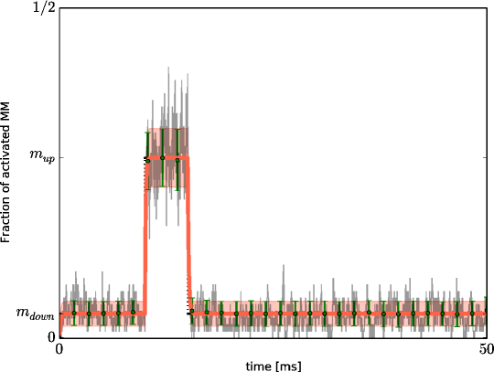
Figure 1: (Left) Schema of the reaction involved in a single receptor site. The two constants $\alpha,\beta$ are the kinetic constants for the release and fixation of the messenger, respectively. (Right) Dynamics of receptor binding when the ligand concentration is increased for 5 ms for a population of 100 receptors. The gray line shows the fraction of bound molecules as simulated with the Gillespie algorithm. The green dots show the ensemble average ($\pm$ one standard deviation) of these trajectories over 500 repetitions. The orange curve shows the same variable as obtained by the continuous time dynamics of the mean and variance (see Section 6.2.2 for the derivation of these equations). Parameters are chosen according to the acetylcholine receptor described in [43] (see Table 1).

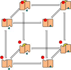
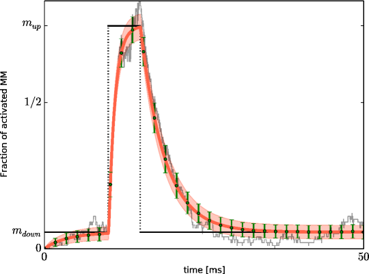
Figure 2: (Left) Schema of a macromolecule with two receptor sites (red circle and green triangle) and one catalytic site (yellow). (Right) Simulation of this macromolecule when the concentrations of both ligands are increased from $2\mu M$ to $20\mu M$ during 5 ms. The vertical axis shows the fraction of activated catalytic sites. The same conventions as in Figure 1 are used for the curves. The black line shows the activated fraction of catalytic sites in the stationary state. See Table 3 for the definition of parameters.

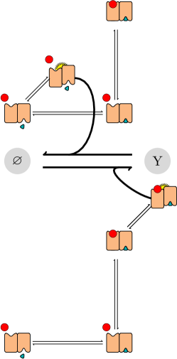
Figure 3: (Left) Reaction schema for the production and removal of $Y$ with both reactions controlled by the catalytic site of a macromolecule. The state diagram for each macromolecule is a restricted version of the cube from Figure 2. Each macromolecule has four allowed states: three inactive states and one active state. For both macromolecules the three inactive states are : no receptor sites bound, green triangle site bound and both bound. The active state of the macromolecule controlling removal of $Y$ (top) has no receptor site bound. The active state of the macromolecule controlling production of $Y$ (bottom) has both receptor sites bound. This cascade implements one of the possible computations listed in Section 4.3.2, the product of the ligands concentrations $y\propto x_{1}.x_{2}$. (Right) Result of the simulations where macromolecule transitions are updated using stochastic simulation and $Y$ production is computed using Euler integration. The surface shows the product of ligand concentrations $x_{1}.x_{2}$ and the wireframe shows the scaled simulated concentration in Y.

References

- 1. Jaynes ET (2003) Probability Theory: the Logic of Science. Cambridge University Press.
- 2. Knill DC, Richards W (1996) Perception as bayesian inference. MIT Press, Cambridge, MA.
- 3. Weiss Y, Simoncelli EP, Adelson EH (2002) Motion illusions as optimal percepts. Nature Neuroscience 5: 598–604.
- 4. Rao R, Olshausen B, Lewicki M (2002) Probabilistic models of the brain: perception and neural function. MIT Press.
- 5. Mamassian P, Landy MS, Maloney LT (2002) Bayesian modelling of visual perception, Rao, R. P. N. and Olshausen, B. A. and Lewicki, M. S. pp. 13–36.
- 6. Ernst MO, Banks MS (2002) Humans integrate visual and haptic information in a statistically optimal fashion. Nature 415: 429-33.
- 7. Laurens J, Droulez J (2007) Bayesian processing of vestibular information. Biological Cybernetics 96: 389–404.
- 8. Körding KP, Wolpert DM (2004) Bayesian integration in sensorimotor learning. Nature 427: 244–7.
- 9. Körding K, Wolpert D (2006) Bayesian decision theory in sensorimotor control. Trends in Cognitive Sciences 10: 320-326.
- 10. Colas F, Droulez J, Wexler M, Bessière P (2008) A unified probabilistic model of the perception of three-dimensional structure from optic flow. Biological Cybernetics : 132–154.
- 11. Todorov E (2008) General duality between optimal control and estimation. In: Proceedings of the 47th IEEE Conference on Proceedings of the 47th IEEE Conference on Decision and Control. pp. 4286-4292.
- 12. Bessière P, Laugier C, Siegwart R (2008) Probabilistic Reasoning and Decision Making in Sensory-Motor Systems. Springer.
- 13. Bessière P, Mazer E, Ahuactzin JM, Mekhnacha K (2013) Bayesian Programming. Chapman and Hall/CRC.
- 14. Pearl J (1988) Probabilistic reasoning in Intelligent Systems: Networks of Plausible Inference. Morgan Kaufmann.
- 15. Zemel R, Dayan P, Pouget A (1998) Probabilistic interpolation of population code. Neural Computation 10: 403-430.
- 16. Deneve S, Latham PE, Pouget A (1999) Reading population codes: a neural implementation of ideal observers. Nat Neurosci 2: 740–745.
- 17. Gold J, Shadlen M (2002) Banburismus and the brain: decoding the relationship between sensory stimuli, decisions, and reward. Neuron 36: 299-308.
- 18. Ma WJ, Beck JM, Pouget A (2008) Spiking networks for bayesian inference and choice. Current Opinion in Neurobiology 18: 217-222.
- 19. Deneve S (2008) Bayesian spiking neurons i: Inference. Neural Computation 20: 91-117.
- 20. Houillon A, Bessière P, Droulez J (2010) The probabilistic cell: Implementation of a probabilistic inference by the biochemical mechanisms of phototransduction. Acta Biotheoretica 58: 103-120.
- 21. Kobayashi TJ (2010) Implementation of dynamic bayesian decision making by intracellular kinetics. Phys Rev Lett 104: 228104.
- 22. Siggia ED, Vergassola M (2013) Decisions on the fly in cellular sensory systems. Proceedings of the National Academy of Sciences 110: E3704-E3712.
- 23. Napp NE, Adams RP (2013) Message passing inference with chemical reaction networks. In: Burges C, Bottou L, Welling M, Ghahramani Z, Weinberger K, editors, Advances in Neural Information Processing Systems 26, Curran Associates, Inc. pp. 2247–2255.
- 24. Monod J, Wyman J, Changeux JP (1965) On the nature of allosteric transitions: A plausible model. Journal of Molecular Biology 12: 88 - 118.
- 25. Changeux JP, Edelstein SJ (2005) Allosteric mechanisms of signal transduction. Science 308: 1424-1428.
- 26. Knapp JE, Pahl R, Šrajer V, Royer WE (2006) Allosteric action in real time: Time-resolved crystallographic studies of a cooperative dimeric hemoglobin. Proceedings of the National Academy of Sciences 103: 7649-7654.
- 27. Elbert R (2007) A milestoning study of the kinetics of an allosteric transition: Atomically detailed simulations of deoxy scapharca hemoglobin. Biophys J 92.
- 28. Triller A, Choquet D (2005) Surface tracking of receptors between synaptic and extrasynaptic membranes: and yet they surface tracking of receptors between synaptic and extrasynaptic membranes: and yet they do move. Trends Neuroscience 28: 133-139.
- 29. Stipanovich A, Valjent E, Matamales M, Nishi A, Ahn JH, et al. (2008) A phosphatase cascade by which rewarding stimuli control nucleosomal response. Nature 453: 879.
- 30. Fernandez E, Schiappa R, Girault JA, Le Novère N (2006) DARPP-32 is a robust integrator of dopamine and glutamate signals. PLoS Computational Biology 2: e176.
- 31. Neher E, Sakmann B (1976) Single-channel currents recorded from membrane of denervated frog muscle fibres. Nature 260.
- 32. Sakmann B, Neher E (1995) Single-Channel Recording. Plenum Press.
- 33. Colquhoun D, Hawkes AG (1981) On the stochastic properties of single ion channels. Proceedings of the Royal Society of London Series B Biological Sciences 211: 205-235.
- 34. Laüger P (1995) Conformational transitions of ionic channels. In: Sakmann B, Neher E, editors, Single-Channel Recording, Plenum Press. pp. 651-662.
- 35. Chung SH, Kennedy RA (1996) Coupled markov chain model: characterization of membrane channel currents with multiple conductance sublevels as partially coupled elementary pores. Math Biosci 133: 111–137.
- 36. Bezanilla F (2000) The voltage sensor in voltage-dependent ion channels. Pysiol Rev 80: 555-592.
- 37. Iseki M, Matsunaga S, Murakami A, Ohno K, Shiga K, et al. (2002) A blue-light-activated adenylyl cyclase mediates photoavoidance in euglena gracilis. Nature 415: 1047–1051.
- 38. Fasano C, Tercé F, Niel JP, Nguyen TTH, Hiol A, et al. (2007) Neuronal conduction of excitation without action potentials based on ceramide production. PLoS ONE 2: e612.
- 39. Stroock DW (2014) An Introduction to Markov Processes. Springer.
- 40. Gillespie DT (1977) Exact stochastic simulation of coupled chemical reactions. The Journal of Physical Chemestry 81: 2340-2361.
- 41. Gillespie DT (2007) Stochastic simulation of chemical kinetics. Annual Review of Physical Chemistry 58: 35-55.
- 42. Gardner CW (2004) Handbook of stochastic methods. Springer, 3rd edition.
- 43. Edelstein SJ, Schaad O, Henry E, Bertrand D, Changeux JP (1996) A kinetic mechanism for nicotinic acetylcholine receptors based on multiple allosteric transitions. Biol Cybern 75: 361–379.