A $L^{\infty}$ bound for the Cahnā€“Hilliard equation with relaxed non-smooth free energy

Christian Kahle
Abstract

Phase field models are widely used to describe multiphase systems. Here a smooth indicator function, called phase field, is used to describe the spatial distribution of the phases under investigation. Material properties like density or viscosity are introduced as given functions of the phase field. These parameters typically have physical bounds to fulfil, e.g. positivity of the density. To guarantee these properties, uniform bounds on the phase field are of interest.

In this work we derive a uniform bound on the solution of the Cahnā€“Hilliard system, where we use the double-obstacle free energy, that is relaxed by Moreauā€“Yosida relaxation.

1 Introduction

Phase field models are a common approach to describe fluid systems of two or more components and to deal with the complex topology changes that might appear in such systems. One of the basic models is the Cahnā€“Hilliard system [CH58] that models spinodal decomposition of a binary metal alloy with components having essentially the same density. Particles are only transported by diffusion. Based on this model several extensions to transport by convection (model ā€™Hā€™ [HH77]) and additionally to fluids with different densities are proposed throughout the literature, see [LT98, Boy02, DSS07, AGG12]. In those models typically the density and viscosity of the two fluid components are introduced as given functions of a phase field that is introduced to describe their spatial distribution and that is the solution of a Cahnā€“Hilliard type equation. In general for the Cahnā€“Hilliard equation with free energies, which allow non-physical values of the phase field, no $L^{\infty}(\Omega)$ bounds are available. As a consequence, in general situations one can not guarantee that the density and the viscosity of the fluids stay positive, i.e. one might run into non-physical data.

In this work we summarize, combine and extend results on the analytical treatment of the Cahnā€“Hilliard equation with double-obstacle free energy, which is relaxed using Moreauā€“Yosida relaxation. The aim of this work is, to help later work on Cahnā€“Hilliard type models by providing $L^{\infty}(\Omega)$ bounds on the violation of the physical meaningful values of the phase field.

Using Moreauā€“Yosida relaxation for the treatment of the Cahnā€“Hilliard equation with double-obstacle free energy is first analytically investigated in [HHT11]. Therein especially the convergence of the solutions of the relaxed system to the solution of the double-obstacle system is shown. One main ingredient is the interpretation of the Cahnā€“Hilliard equation as the first order optimality conditions of a suitable optimal control problem with box constraints in $H^{1}(\Omega)$ on the control.

On the other hand, in [HSW14], a typical optimal control problem with box constraints in $C(\bar{\Omega})$ on the state is investigated. Here the constraints are treated using Moreauā€“Yosida relaxation. The authors provide decay rates for the $L^{\infty}(\Omega)$ norm of the violation of the box constraints in terms of the relaxation parameter. The proof relies on higher regularity of the state, i.e. Hƶlder regularity is used.

The results in [HSW14] apply for the case of Dirichlet boundary data on the state, while in [HKW15] these results are used for the Cahnā€“Hilliard equation with Neumann boundary data, to prove convergence of solutions for a relaxed equation to the solutions of a Cahnā€“Hilliard system with double-obstacle free energy. However, in [HKW15] no convergence rate is provided.

Here we combine the aforementioned results to obtain a $L^{\infty}(\Omega)$ bound on the violation of the physically meaningful values of the solution of the Cahnā€“Hilliard equation that can later be used in more sophisticated models where bounds on parameters, like the density, that depend on the solution of the Cahnā€“Hilliard equation, are required.

The paper is organized as follows. In Section 2 we introduce the time discrete Cahnā€“Hilliard system with double-obstacle free energy and its relaxation using Moreauā€“Yosida relaxation. We further summarize results from [HHT11]. In Section 3 we apply proofs from [HSW14] to obtain a $L^{1}(\Omega)$ bound and based on this a first $L^{\infty}(\Omega)$ bound on the constraint violation. Using a structural assumption, in Section 4 we improve this bound. Finally a numerical validation is carried out in Section 5.

2 The Cahnā€“Hilliard system with double-obstacle free energy

In the following, let $\Omega\subset\mathbb{R}^{n}$, $n\in\{2,3\}$ denote an open bounded domain, that fulfils the cone condition, see [AF03]. Its outer normal we denote by $\nu_{\Omega}$.

We further use usual notation for Sobolev spaces defined on $\Omega$, see [AF03], i.e. $W^{k,p}(\Omega)$ denotes the space of functions that admit weak derivatives up to order $k$ that are Lebesgue-integrable to the power $p$. For $p=2$ we write $H^{k}(\Omega):=W^{k,2}(\Omega)$ and for $k=0$ we write $L^{p}(\Omega):=W^{0,p}(\Omega)$. For $v\in W^{k,p}(\Omega)$ its norm is denoted by $\|v\|_{W^{k,p}(\Omega)}$.

Moreover we introduce

$\displaystyle\mathcal{K}=\{v\in H^{1}(\Omega)\,|\,|v|\leq 1a.e.\},$
$\displaystyle V_{0}=\{v\in H^{1}(\Omega)\,|\,(v,1)=0\}.$

For a fixed time $t$ we consider an alloy consisting of two components $A$ and $B$ and we are interested in the evolution of this alloy over time. For the description of the distribution of the two components we introduce a phase field $\varphi$ that serves as a binary indicator function in the sense, that $\varphi(x)=1$ indicates pure fluid of component $A$ at point $x\in\Omega$, while $\varphi(x)=-1$ indicates pure fluid of component $B$. We further assume, that the transition zone $\Gamma_{\epsilon}$ between $A$ and $B$ is of positive thickness, proportional to $\epsilon$, and that both components are mixed therein. The phase field admits values from the interval $(-1,1)$ in this region.

We introduce the Ginzburgā€“Landau energy of the system by

$\displaystyle GL(\varphi)=\int_{\Omega}\frac{\epsilon}{2}|\nabla\varphi|^{2}+\frac{1}{\epsilon}W(\varphi)\,dx.$

Here $W(\varphi)$ is the so called free energy density and is of double well type, i.e. it admits exactly two minima at $\pm 1$ and is positive everywhere else. We denote the first variation of $GL$ by

$\displaystyle\mu:=-\epsilon\Delta\varphi+\epsilon^{-1}W^{\prime}(\varphi)$

and introduce a mass conserving gradient flow with a mobility or diffusivity $b(\varphi)$ depending of the fluid component as

$\displaystyle\partial_{t}\varphi$ $\displaystyle=\mbox{div}(b(\varphi)\nabla\mu),$ (1)
$\displaystyle-\epsilon\Delta\varphi+\epsilon^{-1}W^{\prime}(\varphi)$ $\displaystyle=\mu.$ (2)

We supplement (1)ā€“(2) with appropriate initial data $\varphi_{0}\in\mathcal{K}$ and boundary data $\nu_{\Omega}\cdot\nabla\varphi=\nu_{\Omega}\cdot\nabla\mu=0$ on $\partial\Omega$. This system is introduced in [CH58] and is called Cahnā€“Hilliard system.

Specific choices of $b(\varphi)$ and $W(\varphi)$ give different analytical difficulties. Here we restrict to the case of non degenerate mobility $b(\varphi)\geq\theta$, for some $\theta>0$, and for simplicity to constant mobility $b(\varphi)\equiv 1$.

For the free energy we choose the double-obstacle free energy introduced in [OP88] and analytically investigated in [BE91]. It has the form

$\displaystyle W(\varphi):=\begin{cases}\frac{1}{2}(1-\varphi^{2})&\mbox{if }|\varphi|\leq 1,\\ +\infty&\mbox{else}.\end{cases}$

Since this $W$ is not smooth, (2) here has the form of a variational inequality, see Definition 1, where we state the precise formulation of the Cahnā€“Hilliard system with constant mobility and double-obstacle free energy.

Definition 1.

Let $\Omega\subset\mathbb{R}^{n}$, $n\in\{2,3\}$, denote a given bounded domain $I=(0,T]$, $T>0$ denote a given time interval. $\varphi_{0}\in\mathcal{K}$ is a given initial phase field.

Then the Cahnā€“Hilliard system with constant mobility and double-obstacle free energy consists in finding a phase field $\varphi$ and a chemical potential $\mu$ such that

$\displaystyle\varphi\in H^{1}(0,T,(H^{1}(\Omega))^{\star})\cap L^{\infty}(0,T,H^{1}(\Omega)),$ (3)
$\displaystyle\mu\in L^{2}(0,T,H^{1}(\Omega)),$
$\displaystyle\varphi(t)\in\mathcal{K}\quad\forall t\in(0,T),$
$\displaystyle(\varphi_{t},v)+(\nabla\mu,\nabla v)=0\quad\forall v\in H^{1}(\Omega),$
$\displaystyle\epsilon(\nabla\varphi,\nabla v-\nabla\varphi)-\epsilon^{-1}(\varphi,v-\varphi)\geq(\mu,v-\varphi)\quad\forall v\in\mathcal{K},$
$\displaystyle\nu_{\Omega}\cdot\nabla\varphi=0\quad\mbox{ on }\partial\Omega,$
$\displaystyle\nu_{\Omega}\cdot\nabla\mu=0\quad\mbox{ on }\partial\Omega,$
$\displaystyle\varphi(0)=\varphi_{0}.$

This system is first investigated in [BE91]. We state the existence and regularity results here.

Theorem 2 ([BE91]).

There exists a unique solution $\varphi,\mu$ to (3) fulfilling $\varphi\in L^{2}(0,T;H^{2}(\Omega))$, $\partial_{\nu_{\Omega}}\varphi=0$ on $\partial\Omega$ for a.e. $t$. It further holds $\forall t>0$ $\min(\sqrt{t},1)\|\varphi(t)\|_{H^{2}(\Omega)}\leq C(\varphi_{0})$, and $\min(\sqrt{t},1)\|\mu(t)\|_{H^{1}(\Omega)}\leq C(\varphi_{0})$.

In this work we deal with the time discrete variant of (3). For this let $0=t_{0}<t_{1}<\ldots<t_{k-1}<t_{k}<\ldots<t_{M}=T$ denote a decomposition of $I=(0,T]$ with time step size $\tau^{k}=t_{k}-t_{k-1}$.

Then the time discrete variant of (3) in weak form consist of finding $(\varphi^{\star},\mu^{\star})\in H^{1}(\Omega)\times H^{1}(\Omega)$ fulfilling

$\displaystyle(\varphi^{\star},v)+\tau^{k}(\nabla\mu^{\star},\nabla v)$ $\displaystyle=(\varphi^{k-1},v)$ $\displaystyle\forall v\in H^{1}(\Omega),$ (4)
$\displaystyle\epsilon(\nabla\varphi^{\star},\nabla v-\nabla\varphi^{\star})-\epsilon^{-1}(\varphi^{k-1},v-\varphi^{\star})$ $\displaystyle\geq(\mu^{\star},v-\varphi^{\star})$ $\displaystyle\forall v\in\mathcal{K}.$ (5)

We further introduce a parameter sā‰«0much-greater-thanš‘ 0s\gg 0 and the penalising function

$\displaystyle\lambda(\varphi)=\lambda_{+}(\varphi)+\lambda_{-}(\varphi):=\max(0,\varphi-1)+\min(0,\varphi+1),$

and define the outer approximation, [GLT81], of (4)ā€“(5) as follows:
Find (Ļ†s,Ī¼s)āˆˆH1ā€‹(Ī©)ƗH1ā€‹(Ī©)superscriptšœ‘š‘ superscriptšœ‡š‘ superscriptš»1Ī©superscriptš»1Ī©(\varphi^{s},\mu^{s})\in H^{1}(\Omega)\times H^{1}(\Omega) fulfilling

(Ļ†s,v)+Ļ„kā€‹(āˆ‡Ī¼s,āˆ‡v)superscriptšœ‘š‘ š‘£superscriptšœš‘˜āˆ‡superscriptšœ‡š‘ āˆ‡š‘£\displaystyle(\varphi^{s},v)+\tau^{k}(\nabla\mu^{s},\nabla v) $\displaystyle=(\varphi^{k-1},v)$ $\displaystyle\forall v\in H^{1}(\Omega),$ (6)
Ļµā€‹(āˆ‡Ļ†s,āˆ‡v)+Ļµāˆ’1ā€‹(sā€‹Ī»ā€‹(Ļ†s),v)āˆ’Ļµāˆ’1ā€‹(Ļ†kāˆ’1,v)italic-Ļµāˆ‡superscriptšœ‘š‘ āˆ‡š‘£superscriptitalic-Ļµ1š‘ šœ†superscriptšœ‘š‘ š‘£superscriptitalic-Ļµ1superscriptšœ‘š‘˜1š‘£\displaystyle\epsilon(\nabla\varphi^{s},\nabla v)+\epsilon^{-1}(s\lambda(\varphi^{s}),v)-\epsilon^{-1}(\varphi^{k-1},v) =(Ī¼s,v)absentsuperscriptšœ‡š‘ š‘£\displaystyle=(\mu^{s},v) $\displaystyle\forall v\in H^{1}(\Omega).$ (7)

Then the following result holds.

Theorem 3 ([HHT11, Thm. 3.2, Thm. 4.1,Thm. 4.2, Lem. 4.3, Thm. 4.4]).

There exist unique solutions $\varphi^{\star},\mu^{\star}$ to (4)ā€“(5) and Ļ†s,Ī¼ssuperscriptšœ‘š‘ superscriptšœ‡š‘ \varphi^{s},\mu^{s} to (6)ā€“(7). Moreover

(Ļ†s,Ī¼s)ā†’(Ļ†ā‹†,Ī¼ā‹†)ā€‹Ā inĀ ā€‹H1ā€‹(Ī©),ā†’superscriptšœ‘š‘ superscriptšœ‡š‘ superscriptšœ‘ā‹†superscriptšœ‡ā‹†Ā inĀ superscriptš»1Ī©\displaystyle(\varphi^{s},\mu^{s})\to(\varphi^{\star},\mu^{\star})\mbox{ in }H^{1}(\Omega),

and there exists a constant $C>0$ independent of sš‘ s such that

ā€–Ļ†sā€–H1ā€‹(Ī©)+sā€‹ā€–Ī»ā€‹(Ļ†s)ā€–L2ā€‹(Ī©)+ā€–Ī¼sā€–H1ā€‹(Ī©)ā‰¤C.subscriptnormsubscriptšœ‘š‘ superscriptš»1Ī©š‘ subscriptnormšœ†subscriptšœ‘š‘ superscriptšæ2Ī©subscriptnormsubscriptšœ‡š‘ superscriptš»1Ī©š¶\displaystyle\|\varphi_{s}\|_{H^{1}(\Omega)}+s\|\lambda(\varphi_{s})\|_{L^{2}(\Omega)}+\|\mu_{s}\|_{H^{1}(\Omega)}\leq C.
Remark 4.

We introduce a free energy density Wsā€‹(Ļ†)=12ā€‹(1āˆ’Ļ†2)+s2ā€‹Ī»ā€‹(Ļ†)2superscriptš‘Šš‘ šœ‘121superscriptšœ‘2š‘ 2šœ†superscriptšœ‘2W^{s}(\varphi)=\frac{1}{2}(1-\varphi^{2})+\frac{s}{2}\lambda(\varphi)^{2}. Then (7) can also be obtained as time discretization of (1)ā€“(2) with this free energy. However, we note that Wssuperscriptš‘Šš‘ W^{s} is not a valid free energy in the sense that its minima are located at Īø=Ā±(1+ssāˆ’1)šœƒplus-or-minus1š‘ š‘ 1\theta=\pm\left(1+\frac{s}{s-1}\right) and attain negative values. After shifting Wssuperscriptš‘Šš‘ W^{s} to have non negative values and scaling its argument by $\theta$, this Wssuperscriptš‘Šš‘ W^{s} might be regarded as a new type of free energy.

From the point of treating variational inequalities, (7) is an outer approximation [GLT81] of (5), while the logarithmic free energy proposed in [CH58] can be regarded as an inner approximation.

3 A first $L^{\infty}$ bound on the constraint violation

In this section we follow the approach in [HSW14, Sec. 2]. Using the uniform boundedness of Ļ†ssuperscriptšœ‘š‘ \varphi^{s} and Ī¼ssuperscriptšœ‡š‘ \mu^{s} from Theorem 3 we first derive $L^{1}(\Omega)$ bounds for the constraints violation Ī»ā€‹(Ļ†s)šœ†superscriptšœ‘š‘ \lambda(\varphi^{s}) that we later use to derive a first bound on ā€–Ī»ā€‹(Ļ†s)ā€–Lāˆžā€‹(Ī©)subscriptnormšœ†superscriptšœ‘š‘ superscriptšæĪ©\|\lambda(\varphi^{s})\|_{L^{\infty}(\Omega)}.

Note that from regularity theory for the Laplace operator with Neumann boundary data, see e.g. [Tay96], we have Ļ†sāˆˆH2ā€‹(Ī©)superscriptšœ‘š‘ superscriptš»2Ī©\varphi^{s}\in H^{2}(\Omega) and from (7) and Theorem 3 it follows that ā€–Ļ†sā€–H2ā€‹(Ī©)subscriptnormsuperscriptšœ‘š‘ superscriptš»2Ī©\|\varphi^{s}\|_{H^{2}(\Omega)} is uniformly bounded in sš‘ s. From Sobolev embedding theory we further have $H^{2}(\Omega)\hookrightarrow C^{0,\beta}(\overline{\Omega})$ for $\beta<2-\frac{n}{2}$, and thus indeed Ī»ā€‹(Ļ†s)āˆˆLāˆžā€‹(Ī©)šœ†superscriptšœ‘š‘ superscriptšæĪ©\lambda(\varphi^{s})\in L^{\infty}(\Omega). From Theorem 3 we further have Ī»ā€‹(Ļ†s)ā†’0ā†’šœ†superscriptšœ‘š‘ 0\lambda(\varphi^{s})\to 0 for sā†’āˆžā†’š‘ s\to\infty, compare also the discussion in [GHK16, Rem. 6].

Theorem 5.

There exists $C>0$ independent of sš‘ s, such that for sā†’āˆžā†’š‘ s\to\infty it holds

ā€–Ī»ā€‹(Ļ†s)ā€–L1ā€‹(Ī©)ā‰¤Cā€‹sāˆ’1.subscriptnormšœ†superscriptšœ‘š‘ superscriptšæ1Ī©š¶superscriptš‘ 1\displaystyle\|\lambda(\varphi^{s})\|_{L^{1}(\Omega)}\leq Cs^{-1}.
Proof.

We test (6) with vā‰”Ī¼sš‘£superscriptšœ‡š‘ v\equiv\mu^{s}, (7) with vā‰”Ļ†sš‘£superscriptšœ‘š‘ v\equiv\varphi^{s} and add the two equations yielding

Ļµāˆ’1ā€‹sā€‹(Ī»ā€‹(Ļ†s),Ļ†s)superscriptitalic-Ļµ1š‘ šœ†superscriptšœ‘š‘ superscriptšœ‘š‘ \displaystyle\epsilon^{-1}s(\lambda(\varphi^{s}),\varphi^{s}) =āˆ’Ļ„kā€‹ā€–āˆ‡Ī¼sā€–2+(Ļ†kāˆ’1,Ī¼s)āˆ’Ļµā€‹ā€–āˆ‡Ļ†sā€–2+Ļµāˆ’1ā€‹(Ļ†kāˆ’1,Ļ†s)absentsuperscriptšœš‘˜superscriptnormāˆ‡superscriptšœ‡š‘ 2superscriptšœ‘š‘˜1superscriptšœ‡š‘ italic-Ļµsuperscriptnormāˆ‡superscriptšœ‘š‘ 2superscriptitalic-Ļµ1superscriptšœ‘š‘˜1superscriptšœ‘š‘ \displaystyle=-\tau^{k}\|\nabla\mu^{s}\|^{2}+(\varphi^{k-1},\mu^{s})-\epsilon\|\nabla\varphi^{s}\|^{2}+\epsilon^{-1}(\varphi^{k-1},\varphi^{s})
$\displaystyle\leq C$

with a $C>0$ independent of sš‘ s by the uniform boundedness of Ļ†ssuperscriptšœ‘š‘ \varphi^{s} and Ī¼ssuperscriptšœ‡š‘ \mu^{s} in $H^{1}(\Omega)$.

By noting Ļ†s>1ā‡”Ī»+ā€‹(Ļ†s)>0ā‡”superscriptšœ‘š‘ 1subscriptšœ†superscriptšœ‘š‘ 0\varphi^{s}>1\Leftrightarrow\lambda_{+}(\varphi^{s})>0 and Ļ†s<āˆ’1ā‡”Ī»āˆ’ā€‹(Ļ†s)<0ā‡”superscriptšœ‘š‘ 1subscriptšœ†superscriptšœ‘š‘ 0\varphi^{s}<-1\Leftrightarrow\lambda_{-}(\varphi^{s})<0, we further have

āˆ«Ī©Ī»+ā€‹(Ļ†s)ā€‹Ļ†sā€‹š‘‘xā‰„āˆ«Ī©|Ī»+ā€‹(Ļ†s)|ā€‹š‘‘x,āˆ«Ī©Ī»āˆ’ā€‹(Ļ†s)ā€‹Ļ†sā€‹š‘‘xā‰„āˆ«Ī©|Ī»āˆ’ā€‹(Ļ†s)|ā€‹š‘‘x,formulae-sequencesubscriptĪ©subscriptšœ†superscriptšœ‘š‘ superscriptšœ‘š‘ differential-dš‘„subscriptĪ©subscriptšœ†superscriptšœ‘š‘ differential-dš‘„subscriptĪ©subscriptšœ†superscriptšœ‘š‘ superscriptšœ‘š‘ differential-dš‘„subscriptĪ©subscriptšœ†superscriptšœ‘š‘ differential-dš‘„\displaystyle\int_{\Omega}\lambda_{+}(\varphi^{s})\varphi^{s}\,dx\geq\int_{\Omega}|\lambda_{+}(\varphi^{s})|\,dx,\quad\int_{\Omega}\lambda_{-}(\varphi^{s})\varphi^{s}\,dx\geq\int_{\Omega}|\lambda_{-}(\varphi^{s})|\,dx,

and thus

Ļµāˆ’1ā€‹sā€‹ā€–Ī»ā€‹(Ļ†s)ā€–L1ā€‹(Ī©)ā‰¤Ļµāˆ’1ā€‹sā€‹(Ī»ā€‹(Ļ†s),Ļ†s)ā‰¤Csuperscriptitalic-Ļµ1š‘ subscriptnormšœ†superscriptšœ‘š‘ superscriptšæ1Ī©superscriptitalic-Ļµ1š‘ šœ†superscriptšœ‘š‘ superscriptšœ‘š‘ š¶\displaystyle\epsilon^{-1}s\|\lambda(\varphi^{s})\|_{L^{1}(\Omega)}\leq\epsilon^{-1}s(\lambda(\varphi^{s}),\varphi^{s})\leq C

which completes the proof. āˆŽ

We next derive a bound on ā€–Ī»ā€‹(Ļ†s)ā€–Lāˆžsubscriptnormšœ†superscriptšœ‘š‘ superscriptšæ\|\lambda(\varphi^{s})\|_{L^{\infty}} in terms of ā€–Ī»ā€‹(Ļ†s)ā€–L1ā€‹(Ī©)subscriptnormšœ†superscriptšœ‘š‘ superscriptšæ1Ī©\|\lambda(\varphi^{s})\|_{L^{1}(\Omega)}. Here we follow [HKW15, Thm. 3.7], where [HSW14, Thm. 2.4] is adapted.

Theorem 6.

It holds

ā€–Ī»ā€‹(Ļ†s)ā€–Lāˆžā€‹(Ī©)ā‰¤Cā€‹(Ī©,n,Ī²)ā€‹ā€–Ī»ā€‹(Ļ†s)ā€–L1ā€‹(Ī©)Ī²Ī²+nsubscriptnormšœ†superscriptšœ‘š‘ superscriptšæĪ©š¶Ī©š‘›š›½superscriptsubscriptnormšœ†superscriptšœ‘š‘ superscriptšæ1Ī©š›½š›½š‘›\displaystyle\|\lambda(\varphi^{s})\|_{L^{\infty}(\Omega)}\leq C(\Omega,n,\beta)\|\lambda(\varphi^{s})\|_{L^{1}(\Omega)}^{\frac{\beta}{\beta+n}}
Proof.

From Ļ†sāˆˆH2ā€‹(Ī©)superscriptšœ‘š‘ superscriptš»2Ī©\varphi^{s}\in H^{2}(\Omega) we have the Hƶlder continuity of Ļ†sāˆˆC0,Ī²ā€‹(Ī©ĀÆ)superscriptšœ‘š‘ superscriptš¶0š›½ĀÆĪ©\varphi^{s}\in C^{0,\beta}(\bar{\Omega}) for $\beta<2-\frac{n}{2}$, and thus there exists $C_{\beta}>0$ independent of sš‘ s with ā€–Ļ†sā€–C0,Ī²ā€‹(Ī©)ā‰¤CĪ²subscriptnormsuperscriptšœ‘š‘ superscriptš¶0š›½Ī©subscriptš¶š›½\|\varphi^{s}\|_{C^{0,\beta}(\Omega)}\leq C_{\beta}.

For fixed sš‘ s we set G+={xāˆˆĪ©|Ļ†sā€‹(x)ā‰„1}superscriptšŗconditional-setš‘„Ī©superscriptšœ‘š‘ š‘„1G^{+}=\{x\in\Omega\,|\,\varphi^{s}(x)\geq 1\} and define $x_{\max}\in G^{+}$ to satisfy

Ļ†sā€‹(xmax)āˆ’1=ā€–Ļ†sāˆ’1ā€–Lāˆžā€‹(G+).superscriptšœ‘š‘ subscriptš‘„1subscriptnormsuperscriptšœ‘š‘ 1superscriptšæsuperscriptšŗ\displaystyle\varphi^{s}(x_{\max})-1=\|\varphi^{s}-1\|_{L^{\infty}(G^{+})}.

We set Gāˆ’={xāˆˆĪ©|Ļ†sā€‹(x)ā‰¤āˆ’1}superscriptšŗconditional-setš‘„Ī©superscriptšœ‘š‘ š‘„1G^{-}=\{x\in\Omega\,|\,\varphi^{s}(x)\leq-1\} and define $x_{\min}\in G^{-}$ to satisfy

āˆ’(Ļ†sā€‹(xmin)+1)=ā€–Ļ†s+1ā€–Lāˆžā€‹(Gāˆ’).superscriptšœ‘š‘ subscriptš‘„1subscriptnormsuperscriptšœ‘š‘ 1superscriptšæsuperscriptšŗ\displaystyle-(\varphi^{s}(x_{\min})+1)=\|\varphi^{s}+1\|_{L^{\infty}(G^{-})}.

Now either Ļ†sā€‹(xmax)āˆ’1ā‰”ā€–Ī»ā€‹(Ļ†s)ā€–Lāˆžā€‹(Ī©)superscriptšœ‘š‘ subscriptš‘„1subscriptnormšœ†superscriptšœ‘š‘ superscriptšæĪ©\varphi^{s}(x_{\max})-1\equiv\|\lambda(\varphi^{s})\|_{L^{\infty}(\Omega)} or āˆ’(Ļ†sā€‹(xmin)+1)ā‰”ā€–Ī»ā€‹(Ļ†s)ā€–Lāˆžā€‹(Ī©)superscriptšœ‘š‘ subscriptš‘„1subscriptnormšœ†superscriptšœ‘š‘ superscriptšæĪ©-(\varphi^{s}(x_{\min})+1)\equiv\|\lambda(\varphi^{s})\|_{L^{\infty}(\Omega)} holds. W.l.o.g. we assume Ļ†sā€‹(xmax)āˆ’1ā‰”ā€–Ī»ā€‹(Ļ†s)ā€–Lāˆžā€‹(Ī©)superscriptšœ‘š‘ subscriptš‘„1subscriptnormšœ†superscriptšœ‘š‘ superscriptšæĪ©\varphi^{s}(x_{\max})-1\equiv\|\lambda(\varphi^{s})\|_{L^{\infty}(\Omega)}.

From the definition of Hƶlder continuity we have

Ļ†sā€‹(x)āˆ’1ā‰„Ļ†sā€‹(xmax)āˆ’1āˆ’ā€–Ļ†sā€–C0,Ī²ā€‹(Ī©)ā€‹|xmaxāˆ’x|Ī².superscriptšœ‘š‘ š‘„1superscriptšœ‘š‘ subscriptš‘„1subscriptnormsuperscriptšœ‘š‘ superscriptš¶0š›½Ī©superscriptsubscriptš‘„š‘„š›½\displaystyle\varphi^{s}(x)-1\geq\varphi^{s}(x_{\max})-1-\|\varphi^{s}\|_{C^{0,\beta}(\Omega)}|x_{\max}-x|^{\beta}.

Thus, for |xmaxāˆ’x|ā‰¤(Ļ†sā€‹(xmax)āˆ’12ā€‹CĪ²)1/Ī²subscriptš‘„š‘„superscriptsuperscriptšœ‘š‘ subscriptš‘„12subscriptš¶š›½1š›½|x_{\max}-x|\leq\left(\frac{\varphi^{s}(x_{\max})-1}{2C_{\beta}}\right)^{1/\beta}

Ļ†sā€‹(x)āˆ’1ā‰„12ā€‹(Ļ†sā€‹(xmax)āˆ’1)>0superscriptšœ‘š‘ š‘„112superscriptšœ‘š‘ subscriptš‘„10\displaystyle\varphi^{s}(x)-1\geq\frac{1}{2}(\varphi^{s}(x_{\max})-1)>0

holds.

The domain $\Omega$ satisfies the cone condition. Thus there exists a cone $K_{r}(x_{\max}):=K(x_{\max})\cap B(x_{\max},r)$ of radius $r$ and with vertex $x_{\max}$ such that $K_{r}(x_{\max})\subset\Omega$. Hence the cone $K_{R}(x_{\max})$ with R:=minā”(r,(ā€–Ī»ā€‹(Ļ†s)ā€–Lāˆžā€‹(Ī©)2ā€‹CĪ²)1/Ī²)assignš‘…š‘Ÿsuperscriptsubscriptnormšœ†superscriptšœ‘š‘ superscriptšæĪ©2subscriptš¶š›½1š›½R:=\min\left(r,\left(\frac{\|\lambda(\varphi^{s})\|_{L^{\infty}(\Omega)}}{2C_{\beta}}\right)^{1/\beta}\right) is contained in $G$.

From this we conclude

ā€–Ī»ā€‹(Ļ†s)ā€–L1ā€‹(Ī©)subscriptnormšœ†superscriptšœ‘š‘ superscriptšæ1Ī©\displaystyle\|\lambda(\varphi^{s})\|_{L^{1}(\Omega)} ā‰„āˆ«KRā€‹(xmax)Ļ†sāˆ’1ā€‹dā€‹xabsentsubscriptsubscriptš¾š‘…subscriptš‘„superscriptšœ‘š‘ 1š‘‘š‘„\displaystyle\geq\int_{K_{R}(x_{\max})}\varphi^{s}-1\,dx
ā‰„āˆ«KRā€‹(xmax)12ā€‹(Ļ†sā€‹(xmax)āˆ’1)ā€‹š‘‘xabsentsubscriptsubscriptš¾š‘…subscriptš‘„12superscriptšœ‘š‘ subscriptš‘„1differential-dš‘„\displaystyle\geq\int_{K_{R}(x_{\max})}\frac{1}{2}(\varphi^{s}(x_{\max})-1)\,dx
=|KRā€‹(xmax)|2ā€‹ā€–Ī»ā€‹(Ļ†s)ā€–Lāˆžā€‹(Ī©)absentsubscriptš¾š‘…subscriptš‘„2subscriptnormšœ†superscriptšœ‘š‘ superscriptšæĪ©\displaystyle=\frac{|K_{R}(x_{\max})|}{2}\|\lambda(\varphi^{s})\|_{L^{\infty}(\Omega)}
ā‰„Cā€‹(Ī©,n)ā€‹(ā€–Ī»ā€‹(Ļ†s)ā€–Lāˆžā€‹(Ī©)2ā€‹CĪ²)n/Ī²ā€‹ā€–Ī»ā€‹(Ļ†s)ā€–Lāˆžā€‹(Ī©)absentš¶Ī©š‘›superscriptsubscriptnormšœ†superscriptšœ‘š‘ superscriptšæĪ©2subscriptš¶š›½š‘›š›½subscriptnormšœ†superscriptšœ‘š‘ superscriptšæĪ©\displaystyle\geq C(\Omega,n)\left(\frac{\|\lambda(\varphi^{s})\|_{L^{\infty}(\Omega)}}{2C_{\beta}}\right)^{n/\beta}\|\lambda(\varphi^{s})\|_{L^{\infty}(\Omega)}
=Cā€‹(Ī©,n,Ī²)ā€‹ā€–Ī»ā€‹(Ļ†s)ā€–Lāˆžā€‹(Ī©)n+Ī²Ī²absentš¶Ī©š‘›š›½subscriptsuperscriptnormšœ†superscriptšœ‘š‘ š‘›š›½š›½superscriptšæĪ©\displaystyle=C(\Omega,n,\beta)\|\lambda(\varphi^{s})\|^{\frac{n+\beta}{\beta}}_{L^{\infty}(\Omega)}

āˆŽ

Corollary 7.

From Theorem 6 we have the following $L^{\infty}$ bounds for the violation of the constraint $|\varphi|\leq 1$.

ā€–Ī»ā€‹(Ļ†s)ā€–Lāˆžā€‹(Ī©)ā‰¤{Cā€‹sāˆ’1/3+Ī³Ā ifĀ ā€‹n=2,Cā€‹sāˆ’1/7+Ī³Ā ifĀ ā€‹n=3,subscriptnormšœ†superscriptšœ‘š‘ superscriptšæĪ©casesš¶superscriptš‘ 13š›¾Ā ifĀ š‘›2š¶superscriptš‘ 17š›¾Ā ifĀ š‘›3\displaystyle\|\lambda(\varphi^{s})\|_{L^{\infty}(\Omega)}\leq\begin{cases}Cs^{-1/3+\gamma}&\mbox{ if }n=2,\\ Cs^{-1/7+\gamma}&\mbox{ if }n=3,\end{cases}

where $0<\gamma\ll 1$.

Proof.

It holds

ā€–Ī»ā€‹(Ļ†s)ā€–Lāˆžā€‹(Ī©)ā‰¤Cā€‹ā€–Ī»ā€‹(Ļ†s)ā€–L1ā€‹(Ī©)Ī²n+Ī²ā‰¤Cā€‹sāˆ’Ī²n+Ī².subscriptnormšœ†superscriptšœ‘š‘ superscriptšæĪ©š¶superscriptsubscriptnormšœ†superscriptšœ‘š‘ superscriptšæ1Ī©š›½š‘›š›½š¶superscriptš‘ š›½š‘›š›½\displaystyle\|\lambda(\varphi^{s})\|_{L^{\infty}(\Omega)}\leq C\|\lambda(\varphi^{s})\|_{L^{1}(\Omega)}^{\frac{\beta}{n+\beta}}\leq Cs^{-\frac{\beta}{n+\beta}}.

For $n=2$ we have $\beta<1$ and thus the first claim.
For $n=3$ we have $\beta<\frac{1}{2}$ and thus the second claim. āˆŽ

4 A structural assumption to improve the $L^{\infty}$ bound

In the previous section we derived a bound of the violation ā€–Ī»ā€‹(Ļ†s)ā€–Lāˆžā€‹(Ī©)subscriptnormšœ†superscriptšœ‘š‘ superscriptšæĪ©\|\lambda(\varphi^{s})\|_{L^{\infty}(\Omega)} based on its ā€–Ī»ā€‹(Ļ†s)ā€–L1ā€‹(Ī©)subscriptnormšœ†superscriptšœ‘š‘ superscriptšæ1Ī©\|\lambda(\varphi^{s})\|_{L^{1}(\Omega)} norm. We now state an assumption on the order of ā€–Ī»ā€‹(Ļ†s)ā€–L1ā€‹(Ī©)subscriptnormšœ†superscriptšœ‘š‘ superscriptšæ1Ī©\|\lambda(\varphi^{s})\|_{L^{1}(\Omega)} to obtain an improved $L^{\infty}(\Omega)$ bound.

Assumption 1 ([HSW14, Ass. 2.13]).

For $x\in\Omega$ we assume that there exists $0<K<\infty$, independent of $x,R$, and sš‘ s such that

āˆ«BRā€‹(x)sā€‹|Ī»ā€‹(Ļ†s)|ā€‹š‘‘xā‰¤Kā€‹Rnsubscriptsubscriptšµš‘…š‘„š‘ šœ†superscriptšœ‘š‘ differential-dš‘„š¾superscriptš‘…š‘›\displaystyle\int_{B_{R}(x)}s|\lambda(\varphi^{s})|\,dx\leq KR^{n}

holds.

This assumption states, that G={xāˆˆĪ©|Ī»ā€‹(Ļ†sā€‹(x))ā‰ 0}šŗconditional-setš‘„Ī©šœ†superscriptšœ‘š‘ š‘„0G=\{x\in\Omega\,|\,\lambda(\varphi^{s}(x))\neq 0\} is a subset of $\Omega$ that has a measure comparable to the measure of $\Omega$ and is not a lower dimensional manifold. This is a reasonable assumption since in our application $G$ describes the bulk phases which fill most parts of the domain.

Theorem 8.

Let Assumption 1 hold. Then it holds

ā€–Ī»ā€‹(Ļ†s)ā€–Lāˆžā€‹(Ī©)ā‰¤Cā€‹(Ī©,n,Ī²,K)ā€‹sāˆ’1.subscriptnormšœ†superscriptšœ‘š‘ superscriptšæĪ©š¶Ī©š‘›š›½š¾superscriptš‘ 1\displaystyle\|\lambda(\varphi^{s})\|_{L^{\infty}(\Omega)}\leq C(\Omega,n,\beta,K)s^{-1}.
Proof.

Using Assumption 1 in the proof of Theorem 6 we obtain

Kā€‹sāˆ’1ā€‹Rnš¾superscriptš‘ 1superscriptš‘…š‘›\displaystyle Ks^{-1}R^{n} ā‰„ā€–Ī»ā€‹(Ļ†s)ā€–L1ā€‹(Ī©)absentsubscriptnormšœ†superscriptšœ‘š‘ superscriptšæ1Ī©\displaystyle\geq\|\lambda(\varphi^{s})\|_{L^{1}(\Omega)}
ā‰„Cā€‹(Ī©,n,Ī²)ā€‹ā€–Ī»ā€‹(Ļ†s)ā€–Lāˆžā€‹(Ī©)Ī²+nĪ²absentš¶Ī©š‘›š›½superscriptsubscriptnormšœ†superscriptšœ‘š‘ superscriptšæĪ©š›½š‘›š›½\displaystyle\geq C(\Omega,n,\beta)\|\lambda(\varphi^{s})\|_{L^{\infty}(\Omega)}^{\frac{\beta+n}{\beta}}

Restating the definition of R:=minā”(r,(ā€–Ī»ā€‹(Ļ†s)ā€–Lāˆžā€‹(Ī©)2ā€‹CĪ²)1/Ī²)assignš‘…š‘Ÿsuperscriptsubscriptnormšœ†superscriptšœ‘š‘ superscriptšæĪ©2subscriptš¶š›½1š›½R:=\min\left(r,\left(\frac{\|\lambda(\varphi^{s})\|_{L^{\infty}(\Omega)}}{2C_{\beta}}\right)^{1/\beta}\right) and solving for ā€–Ī»ā€‹(Ļ†s)ā€–Lāˆžā€‹(Ī©)subscriptnormšœ†superscriptšœ‘š‘ superscriptšæĪ©\|\lambda(\varphi^{s})\|_{L^{\infty}(\Omega)} we obtain

ā€–Ī»ā€‹(Ļ†s)ā€–Lāˆžā€‹(Ī©)ā‰¤Cā€‹(Ī©,n,Ī²,K)ā€‹sāˆ’1.subscriptnormšœ†superscriptšœ‘š‘ superscriptšæĪ©š¶Ī©š‘›š›½š¾superscriptš‘ 1\displaystyle\|\lambda(\varphi^{s})\|_{L^{\infty}(\Omega)}\leq C(\Omega,n,\beta,K)s^{-1}. (8)

āˆŽ

Note that this bound is significantly better than the one shown in Theorem 6 and especially is independent of the dimension $n$ of the domain $\Omega$ and of the Hƶlder exponent $\beta$ of Ļ†ssuperscriptšœ‘š‘ \varphi^{s}.

Remark 9.

In (7) we use the violation Ī»ā€‹(Ļ†s)šœ†superscriptšœ‘š‘ \lambda(\varphi^{s}) as penalisation for the outer approximation of the variational inequality (5). The function $\lambda$ is Lipschitz continuous, i.e. $\lambda\in C^{0,1}(\mathbb{R})$. We introduce smoother penalisations by using higher powers of $\lambda$, i.e. for $k\geq 2$ we define

Ī»kā€‹(Ļ†s):=Ī»ā€‹(Ļ†s)ā€‹|Ī»ā€‹(Ļ†s)|kāˆ’2.assignsubscriptšœ†š‘˜superscriptšœ‘š‘ šœ†superscriptšœ‘š‘ superscriptšœ†superscriptšœ‘š‘ š‘˜2\displaystyle\lambda_{k}(\varphi^{s}):=\lambda(\varphi^{s})|\lambda(\varphi^{s})|^{k-2}.

Note that Ī»2ā€‹(Ļ†s)ā‰”Ī»ā€‹(Ļ†s)subscriptšœ†2superscriptšœ‘š‘ šœ†superscriptšœ‘š‘ \lambda_{2}(\varphi^{s})\equiv\lambda(\varphi^{s}) and that it holds $\lambda_{k}\in C^{k-2,1}(B)$ for each bounded interval $B\subset\mathbb{R}$. Further we have at least Ļ†sāˆˆH1ā€‹(Ī©)ā†ŖLqā€‹(Ī©)superscriptšœ‘š‘ superscriptš»1Ī©ā†Ŗsuperscriptšæš‘žĪ©\varphi^{s}\in H^{1}(\Omega)\hookrightarrow L^{q}(\Omega) for $q<6$ if $n\equiv 3$ and $q<\infty$ for $n\equiv 2$. Thus these higher powers of $\lambda$ are still integrable.

Using $\lambda_{k}$ instead of $\lambda$ in (7) leads to the same results, but with $\lambda$ substituted by $\lambda_{k}$. Especially we obtain

ā€–Ī»kā€‹(Ļ†s)ā€–Lāˆžā€‹(Ī©)=ā€–Ī»ā€‹(Ļ†s)kāˆ’1ā€–Lāˆžā€‹(Ī©)ā‰¤Cā€‹sāˆ’1subscriptnormsubscriptšœ†š‘˜superscriptšœ‘š‘ superscriptšæĪ©subscriptnormšœ†superscriptsuperscriptšœ‘š‘ š‘˜1superscriptšæĪ©š¶superscriptš‘ 1\displaystyle\|\lambda_{k}(\varphi^{s})\|_{L^{\infty}(\Omega)}=\|\lambda(\varphi^{s})^{k-1}\|_{L^{\infty}(\Omega)}\leq Cs^{-1} (9)

and thus

ā€–Ī»ā€‹(Ļ†s)ā€–Lāˆžā€‹(Ī©)ā‰¤Cā€‹sāˆ’1kāˆ’1subscriptnormšœ†superscriptšœ‘š‘ superscriptšæĪ©š¶superscriptš‘ 1š‘˜1\displaystyle\|\lambda(\varphi^{s})\|_{L^{\infty}(\Omega)}\leq Cs^{-\frac{1}{k-1}}

Such penalisations with smoother functions might be of interest for optimal control problems, [HK11, HKW15], where sufficient differentiability properties are required, or in the context of model order reduction using proper orthogonal decomposition, [Vol11].

4.1 The fully discrete case

We assume, that $\Omega$ is polygonally bounded and thus can be represented exactly by a finite number of triangles if $n=2$, resp. tetrahedrons if $n=3$. We introduce a subdivision $\mathcal{T}$ of $\Omega$ using triangles, resp. tetrahedrons, and define the space of piecewise linear and globally continuous finite elements as

$\displaystyle V_{h}=\{v\in C(\bar{\Omega})\,|\,v|_{T}\in P^{1}(T)\,\forall T\in\mathcal{T}\}=\mbox{span}\{\phi_{i}\,|\,i=1,\ldots,N\},$

where $P^{1}(T)$ denotes the space of all polynomials defined on $T$ up to order 1. Note that functions from $V_{h}$ are Hƶlder continuous with exponent $\beta<1$.

The discrete counterparts Ļ†hs,Ī¼hssubscriptsuperscriptšœ‘š‘ ā„Žsubscriptsuperscriptšœ‡š‘ ā„Ž\varphi^{s}_{h},\mu^{s}_{h} of Ļ†s,Ī¼ssuperscriptšœ‘š‘ superscriptšœ‡š‘ \varphi^{s},\mu^{s} then fulfil the equations

(Ļ†hs,v)+Ļ„kā€‹(āˆ‡Ī¼hs,āˆ‡v)subscriptsuperscriptšœ‘š‘ ā„Žš‘£superscriptšœš‘˜āˆ‡subscriptsuperscriptšœ‡š‘ ā„Žāˆ‡š‘£\displaystyle(\varphi^{s}_{h},v)+\tau^{k}(\nabla\mu^{s}_{h},\nabla v) $\displaystyle=(\varphi^{k-1},v)$ $\displaystyle\forall v\in V_{h},$
$\displaystyle\epsilon(\nabla(\varphi^{s}_{h},\nabla v)+\epsilon^{-1}\Lambda(\varphi^{s}_{h},v)-\epsilon^{-1}(\varphi^{k-1},v)$ =(Ī¼hs,v)absentsubscriptsuperscriptšœ‡š‘ ā„Žš‘£\displaystyle=(\mu^{s}_{h},v) $\displaystyle\forall v\in V_{h},$

where we investigate three choices for the numerical treatment of the penalisation term Ī›kā€‹(Ļ†hs,v)subscriptĪ›š‘˜subscriptsuperscriptšœ‘š‘ ā„Žš‘£\Lambda_{k}(\varphi^{s}_{h},v). Using linear elements the term Ī›ā€‹(Ļ†hs,v)=Ī›Eā€‹(Ļ†hs,v):=(sā€‹Ī»ā€‹(Ļ†hs),v)Ī›subscriptsuperscriptšœ‘š‘ ā„Žš‘£subscriptĪ›šøsubscriptsuperscriptšœ‘š‘ ā„Žš‘£assignš‘ šœ†subscriptsuperscriptšœ‘š‘ ā„Žš‘£\Lambda(\varphi^{s}_{h},v)=\Lambda_{E}(\varphi^{s}_{h},v):=(s\lambda(\varphi^{s}_{h}),v) can be evaluated exactly. Another possibility is to use the Lagrangian interpolation $I$ for Ī»ā€‹(Ļ†hs)šœ†subscriptsuperscriptšœ‘š‘ ā„Ž\lambda(\varphi^{s}_{h}), i.e. Ī›ā€‹(Ļ†hs,v)=Ī›Iā€‹(Ļ†hs,v):=(sā€‹Iā€‹(Ī»ā€‹(Ļ†hs)),v)Ī›subscriptsuperscriptšœ‘š‘ ā„Žš‘£subscriptĪ›š¼subscriptsuperscriptšœ‘š‘ ā„Žš‘£assignš‘ š¼šœ†subscriptsuperscriptšœ‘š‘ ā„Žš‘£\Lambda(\varphi^{s}_{h},v)=\Lambda_{I}(\varphi^{s}_{h},v):=(sI(\lambda(\varphi^{s}_{h})),v). As last variant we investigate an evaluation using lumping, i.e. Ī›ā€‹(Ļ†hs,v)=Ī›Lā€‹(Ļ†hs,v):=(sā€‹Ī»ā€‹(Ļ†hs),v)hĪ›subscriptsuperscriptšœ‘š‘ ā„Žš‘£subscriptĪ›šæsubscriptsuperscriptšœ‘š‘ ā„Žš‘£assignsuperscriptš‘ šœ†subscriptsuperscriptšœ‘š‘ ā„Žš‘£ā„Ž\Lambda(\varphi^{s}_{h},v)=\Lambda_{L}(\varphi^{s}_{h},v):=(s\lambda(\varphi^{s}_{h}),v)^{h}, where $(v,w)^{h}$ is defined as

$\displaystyle(v,w)^{h}:=\sum_{i=1}^{N}(1,\phi_{i})v(x_{i})w(x_{i}),$

and $x_{i}$ stands for the vertices of $\mathcal{T}$.

Note that |Iā€‹(Ī»ā€‹(Ļ†hs))|ā‰„|Ī»ā€‹(Ļ†hs)|š¼šœ†subscriptsuperscriptšœ‘š‘ ā„Žšœ†subscriptsuperscriptšœ‘š‘ ā„Ž|I(\lambda(\varphi^{s}_{h}))|\geq|\lambda(\varphi^{s}_{h})| and ā€–Iā€‹(Ī»ā€‹(Ļ†hs))ā€–Lāˆžā€‹(Ī©)ā‰”ā€–Ī»ā€‹(Ļ†hs)ā€–Lāˆžā€‹(Ī©)subscriptnormš¼šœ†subscriptsuperscriptšœ‘š‘ ā„ŽsuperscriptšæĪ©subscriptnormšœ†subscriptsuperscriptšœ‘š‘ ā„ŽsuperscriptšæĪ©\|I(\lambda(\varphi^{s}_{h}))\|_{L^{\infty}(\Omega)}\equiv\|\lambda(\varphi^{s}_{h})\|_{L^{\infty}(\Omega)} due to the linear finite elements that we use.

Using the different variants of $\Lambda$ the results from Section 3 and Section 4 stay valid for the fully discrete case, with small changes that we comment on next.

For $\Lambda_{E}$ no changes are required. For $\Lambda_{I}$ and $\Lambda_{L}$ we obtain from Theorem 5

Ļµāˆ’1ā€‹sā€‹ā€–Ī»ā€‹(Ļ†hs)ā€–L1ā€‹(Ī©)ā‰¤Ļµāˆ’1ā€‹sā€‹ā€–Iā€‹(Ī»ā€‹(Ļ†hs))ā€–L1ā€‹(Ī©)ā‰¤C.superscriptitalic-Ļµ1š‘ subscriptnormšœ†subscriptsuperscriptšœ‘š‘ ā„Žsuperscriptšæ1Ī©superscriptitalic-Ļµ1š‘ subscriptnormš¼šœ†subscriptsuperscriptšœ‘š‘ ā„Žsuperscriptšæ1Ī©š¶\displaystyle\epsilon^{-1}s\|\lambda(\varphi^{s}_{h})\|_{L^{1}(\Omega)}\leq\epsilon^{-1}s\|I(\lambda(\varphi^{s}_{h}))\|_{L^{1}(\Omega)}\leq C.

The according $L^{\infty}(\Omega)$ bounds for Ī»ā€‹(Ļ†hs)šœ†subscriptsuperscriptšœ‘š‘ ā„Ž\lambda(\varphi^{s}_{h}) in (8) then follow immediately.

5 Numerical validation

In this section we perform numerical tests to validate the bounds that we found in Theorem 8.

We perform simulations in two and three space dimensions, using $\Omega=(0,1)^{n}$, i.e. the unit square for $n=2$, and the unit cube for $n=3$.

We perform one time step of (6)ā€“(7) and measure the violation ā€–Ī»ā€‹(Ļ†s)ā€–Lāˆžā€‹(Ī©)subscriptnormšœ†superscriptšœ‘š‘ superscriptšæĪ©\|\lambda(\varphi^{s})\|_{L^{\infty}(\Omega)}. The parameter are given as $\epsilon=0.01$ and $\tau=0.01$ if $n=2$ and $\epsilon=0.04$ and $\tau=0.01$ if $n=3$. The initial phase field $\varphi_{0}$ is defined as

$\displaystyle\varphi_{0}(x)$ $\displaystyle=\begin{cases}1&\mbox{ if }z\geq\frac{\pi}{2},\\ -1&\mbox{ if }z\leq-\frac{\pi}{2},\\ \sin(z)&\mbox{ else, }\end{cases}$

where $z=\epsilon^{-1}(\|x-m\|-r)$, and $m=(0.5,0.5)$ for $n=2$ and $m=(0.5,0.5,0.5)$ if $n=3$. This defines a sphere with radius $r=0.25$. Note that the sinus is the principle shape of the phase field across the interface for the double-obstacle free energy [ESSW11].

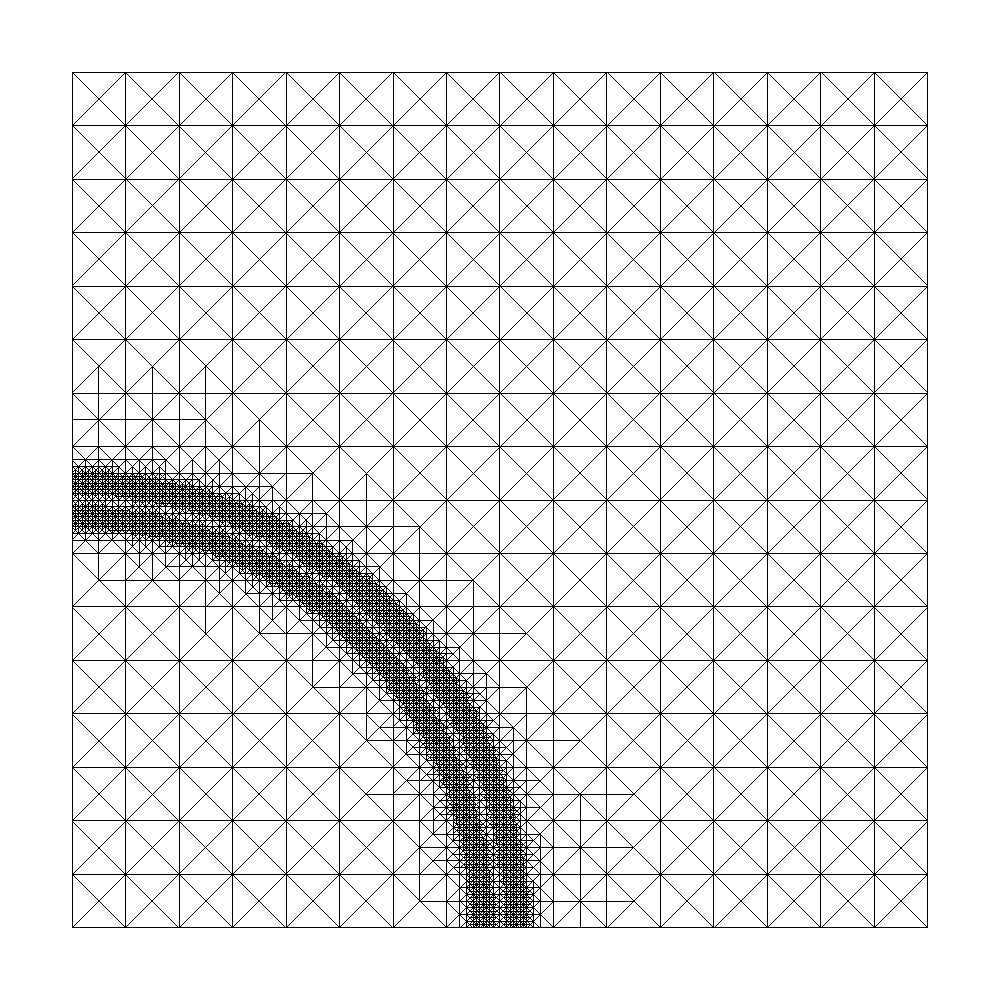
We adapt the mesh for the phase field and the chemical potential by using the reliable and efficient residual based error estimator proposed in [HHT11]. Here we only use the norm of the jumps of the normal derivatives of Ļ†hssuperscriptsubscriptšœ‘ā„Žš‘ \varphi_{h}^{s} and Ī¼hssubscriptsuperscriptšœ‡š‘ ā„Ž\mu^{s}_{h} across edges for $n=2$, resp. faces for $n=3$, which contains the main part of the indicator [CV99]. For the marking of cells we follow [HHT11], i.e. we the procedure proposed by Dƶrfer [Dƶr96].

We perform the usual ā€œsolve$\to$estimate$\to$mark$\to$refineā€ cycle three times for each value of sš‘ s and reuse the final mesh as initial mesh for the next larger value of sš‘ s. In Figure 1 we show a typically mesh obtained by this adaptive solving procedure.

Refer to caption
Figure 1: One quarter of the computational domain for the 2d simulation.

The non linear system (6)ā€“(7) is solved using Newtonā€™s method and the linear systems are solved directly. The implementation is done in C++ using the finite element toolbox FEniCS [LMW12] with the PETSc [BAA+14] linear algebra back end and the MUMPS [ADKL01] direct solver.

Experiments in two space dimensions

In two space dimensions we investigate the three cases of numerical treatment of the penalisation Ī»ā€‹(Ļ†s)šœ†superscriptšœ‘š‘ \lambda(\varphi^{s}) as proposed in Section 4.1, namely the exact integration, the interpolation case and the lumping case.

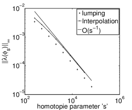
In Figure 2 we present numerical results. We show the violation ā€–Ī»ā€‹(Ļ†s)ā€–Lāˆžā€‹(Ī©)subscriptnormšœ†superscriptšœ‘š‘ superscriptšæĪ©\|\lambda(\varphi^{s})\|_{L^{\infty}(\Omega)} for the different numerical treatments of terms involving $\lambda$.

Refer to caption
Figure 2: The violation of the bound $|\varphi|\leq 1$ for penalisation with $\lambda_{2}$, and the different numerical treatments, i.e. exact evaluation, lumping and interpolation. Note that Newtonā€™s method failed in calculating the solution for larger values of sš‘ s if interpolation is used.

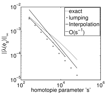
In the case of interpolation we see that Newtonā€™s method is not successful in finding the solution to (6)ā€“(7) for large values of sš‘ s, while the exact evaluation and also the lumping evaluation converge equally well. In the case of exact integration we have a slightly higher violation of the constraints. However in all three cases the theoretical bound from Theorem 8 holds.
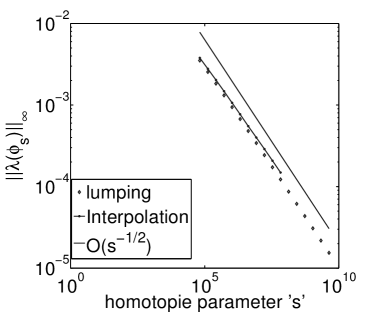
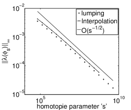
Refer to caption
Refer to caption
Figure 3: The violation of the bound $|\varphi|\leq 1$ for penalisation with $\lambda_{k}$, $k=3,4$ (left to right) and the different numerical treatments, i.e. lumping and interpolation. Note that in both cases, Newtonā€™s method fails in calculating the solution for larger values of sš‘ s if interpolation is used.

As next test we investigate ā€–Ī»ā€‹(Ļ†s)ā€–Lāˆžā€‹(Ī©)subscriptnormšœ†superscriptšœ‘š‘ superscriptšæĪ©\|\lambda(\varphi^{s})\|_{L^{\infty}(\Omega)} when $\lambda_{k}$ for $k>2$ is used for penalisation as proposed in Remark 9. Here we do not perform exact integration.

Also in the case of higher powers of $\lambda$ the theoretical bounds are attained. Again we observe that Newtonā€™s method fails in finding the solution for large values of sš‘ s if interpolation is used, while with lumped evaluation the solution is always found. Note that to obtain comparable violations for $\lambda_{k}$ we need larger values of sš‘ s.

Experiments in three space dimensions

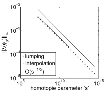
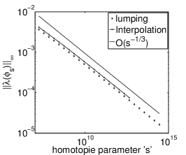
In three dimensions we only investigate lumping and interpolation as treatment of the term with $\lambda$ and again we use $\lambda_{k}$ for $k=2,3,4$.

In Figure 4 we show the numerical results. Again we obtain the expected bounds. Also using interpolation Newtonā€™s method fails in finding the unique solution for larger values of sš‘ s.

Refer to caption
Refer to caption
Refer to caption
Figure 4: Numerical results for three space dimensions and with $\lambda_{k}$, $k=2,3,4$ (left to right). The proposed convergence rate is obtained and again in the case of interpolation of $\lambda$ Newtonā€™s method fails in finding the solution for large values of sš‘ s.

References

  • [ADKL01] P.R. Amestoy, I.S. Duff, J.Ā Koster, and J.-Y. Lā€™Excellent. A fully asynchronous multifrontal solver using distributed dynamic scheduling. SIAM Journal of Matrix Analysis and Applications, 23(1):15ā€“41, 2001.
  • [AF03] R.Ā A. Adams and J.Ā H.Ā F. Fournier. Sobolev Spaces, second edition, volume 140 of Pure and Applied Mathematics. Elsevier, 2003.
  • [AGG12] H.Ā Abels, H.Ā Garcke, and G.Ā GrĆ¼n. Thermodynamically consistent, frame indifferent diffuse interface models for incompressible two-phase flows with different densities. Mathematical Models and Methods in Applied Sciences, 22(3):40, March 2012.
  • [BAA+14] S.Ā Balay, S.Ā Abhyankar, M.F. Adams, J.Ā Brown, P.Ā Brune, K.Ā Buschelman, L.Ā Dalcin, V.Ā Eijkhout, W.D. Gropp, D.Ā Kaushik, M.G. Knepley, L.C. McInnes, K.Ā Rupp, B.F. Smith, S.Ā Zampini, and H.Ā Zhang. PETSc Web page. \urlhttp://www.mcs.anl.gov/petsc, 2014.
  • [BE91] J.Ā F. Blowey and C.Ā M. Elliott. The Cahnā€“Hilliard gradient theory for phase separation with non-smooth free energy. Part I: Mathematical analysis. European Journal of Applied Mathematics, 2:233ā€“280, 1991.
  • [Boy02] F.Ā Boyer. A theoretical and numerical model for the study of incompressible mixture flows. Computers & Fluids, 31(1):41ā€“68, January 2002.
  • [CH58] J.Ā W. Cahn and J.Ā E. Hilliard. Free Energy of a Nonuniform System. I. Interfacial Free Energy. The Journal of Chemical Physics, 28(2):258ā€“267, 1958.
  • [CV99] C.Ā Carstensen and R.Ā VerfĆ¼rth. Edge Residuals Dominate A Posteriori Error Estimates for Low Order Finite Element Methods. SIAM Journal on Numerical Analysis, 36(5):1571ā€“1587, 1999.
  • [Dƶr96] W.Ā Dƶrfler. A convergent adaptive algorithm for Poissonā€™s equation. SIAM Journal on Numerical Analysis, 33(3):1106ā€“1124, 1996.
  • [DSS07] H.Ā Ding, P.Ā D.Ā M. Spelt, and C.Ā Shu. Diffuse interface model for incompressible two-phase flows with large density ratios. Journal of Computational Physics, 226(2):2078ā€“2095, October 2007.
  • [ESSW11] C.M. Elliott, B.Ā Stinner, V.Ā Styles, and R.Ā Welford. Numerical computation of advection and diffusion on evolving diffuse interfaces. IMA Journal of Numerical Analysis, 31(3):786ā€“812, July 2011.
  • [GHK16] H.Ā Garcke, M.Ā Hinze, and C.Ā Kahle. A stable and linear time discretization for a thermodynamically consistent model for two-phase incompressible flow. Applied Numerical Mathematics, 99:151ā€“171, January 2016.
  • [GLT81] R.Ā Glowinski, J.-L. Lions, and R.Ā TrĆ©moliĆ©res. Numerical Analysis of Variational Inequalities, volumeĀ 8 of Studies in Mathematics and its Applications. North-Holland Publishing Company, 1981.
  • [HH77] P.Ā C. Hohenberg and B.Ā I. Halperin. Theory of dynamic critical phenomena. Reviews of Modern Physics, 49(3):435ā€“479, 1977.
  • [HHT11] M.Ā HintermĆ¼ller, M.Ā Hinze, and M.Ā H. Tber. An adaptive finite element Moreauā€“Yosida-based solver for a non-smooth Cahnā€“Hilliard problem. Optimization Methods and Software, 25(4-5):777ā€“811, 2011.
  • [HK11] M.Ā HintermĆ¼ller and I.Ā Kopacka. A smooth penalty approach and a nonlinear multigrid algorithm for elliptic MPECS . Comput. Optim. Appl., 50(1):111ā€“145, 2011.
  • [HKW15] M.Ā HintermĆ¼ller, T.Ā Keil, and D.Ā Wegner. Optimal Control of a Semidiscrete Cahn-Hilliard-Navier-Stokes System with Non-Matched Fluid Densities. arXiv: 1506.03591, 2015.
  • [HSW14] M.Ā HintermĆ¼ller, A.Ā Schiela, and W.Ā Wollner. The Length of the Primal-Dual Path in Moreauā€“Yosida-Based Path-Following Methods for State Constrained Optimal Control. SIAM Journal on Optimization, 24(1):108ā€“126, 2014.
  • [LMW12] A.Ā Logg, K.-A. Mardal, and G.Ā Wells, editors. Automated Solution of Differential Equations by the Finite Element Method - The FEniCS Book, volumeĀ 84 of Lecture Notes in Computational Science and Engineering. Springer, 2012.
  • [LT98] J.Ā Lowengrub and L.Ā Truskinovsky. Quasi-incompressible Cahnā€“Hilliard fluids and topological transitions. Proceedings of the royal society A, 454(1978):2617ā€“2654, 1998.
  • [OP88] Y.Ā Oono and S.Ā Puri. Study of phase-separation dynamics by use of cell dynamical systems. I. Modeling. Physical Review A, 38(1):434ā€“463, 1988.
  • [Tay96] M.Ā E. Taylor. Partial Differential Equations I: Basic Theory, volume 115 of Applied Mathematical Sciences. Springer, 1996.
  • [Vol11] S.Ā Volkwein. Model reduction using proper orthogonal decomposition. lecture script, UniversitƤt Konstanz, 2011.