Observables and initial conditions for rotating and expanding fireballs with spheroidal symmetry

Abstract

Utilizing a recently found class of exact, analytic rotating solutions of non-relativistic fireball hydrodynamics, we calculate analytically the single-particle spectra, the elliptic flows and two-particle Bose-Einstein correlation functions for rotating and expanding fireballs with spheroidal symmetry. We demonstrate, that rotation generates final state momentum anisotropies even for a spatially symmetric, spherical initial geometry of the fireball. The mass dependence of the effective temperatures, as well as the HBT radius parameters and the elliptic flow are shown to be sensitive not only to radial flow effects but also to the magnitude of the initial angular momentum.

I Introduction

In non-central heavy ion collisions, the impact parameter is non-vanishing, and the initial conditions include a non-vanishing, but frequently neglected initial angular momentum of the nucleons that participate in the inelastic collisions. This non-zero initial angular momentum of the participant zone is a conserved quantity that survives the initial, non-equilibrium stage of the heavy ion collision, that results in thermalization. The fireballs created in non-central high energy heavy ion collisions will thus not only expand but rotate as well. The vast majority of numerical and analytic hydrodynamical calculations performed so far completely neglected the effect of the initial angular momentum on the final state observables. The effects of rotation, however, may be rather significant and, rather recently, the imprints of rotation on the observables started to draw significant theoretical attention.

As far as we know, the initial angular momentum of non-central heavy ion collisions was first taken into account in ref. Csernai:2011gg , where a sign change of the directed flow $v_{1}$ was predicted and related to the change of the relative importances of the angular momentum driven expansion to the pressure driven radial expansion. The rotation effect was also related to a rapidity dependent oscillating pattern of the elliptic flows when the fluctuations of the initial center-of-mass rapidity are corrected for. These results were highlighted as an important feature of the description of the nearly perfect fluids formed in high energy heavy ion reactions at RHIC and LHC energies using a numerical hydrodynamical model, that is based on the particle in cell method Cifarelli:2012zz . This hydrodynamical model is a three-dimensional, finite calculation, and it was tested against numerical viscosity and entropy production artefacts  Csernai:2011gg . The finiteness of the fireball is an important requirement, when rotation effects are considered, given that models that assume longitudinal boost invariance and flat rapidity dependence have infinite moment of interia in the beam direction, hence they cannot, by definition, take into account the explosion and simultaneous rotation of the fireball in the impact parameter plane. Such a rotation, by definition, would require a time dependent and finite moment of inertia.

The differential two-particle Bose-Einstein or Hanbury Brown – Twiss correlation function (DHBT) was proposed as an effective tool to measure the angular momentum of non-central heavy ion collisions  Csernai:2013vda . The results detailed in ref. Csernai:2013uda indicated that the DHBT method can indeed be used to detect the angular momentum and the rotation of the fireball, but the effects of irregular initial shapes, density fluctuations, irregular radial flows require extended analysis to disentangle these effects from one another. The differential correlation function was numerically found to dependent on the shape, the temperature, the radial velocity and the angular velocity as well as on the detector position, as it was demonstrated in refs. Velle:2015xha , and the numerical value of the DHBT correlation function for realistic angular velocities and radial flows was found to be rather small, of the order of 2-3 % . Increased initial angular momentum of the rotating and expanding fireball was shown to result in an effective decrease of the observable correlation radii in ref. Velle:2015dpa .

These numerical evaluations of observable signals of a non-vanishing initial angular momentum were partially based on a recently discovered family of exact solutions of rotating and expanding, non-relativistic fireball hydrodynamics, detailed in ref. Csorgo:2013ksa . This solution with non-vanishing initial angular momentum can be considered as the rotating and spheroidally symmetric generalizations of the radially expanding, finite, Gaussian exact solution of fireball hydrodynamics found already in 1998 Csizmadia:1998ef . That solution was shown to be a simultaneous solution of the equations of non-relativistic fireball hydrodynamics with spheroidal symmetry, and at the same time, also a solution of the non-relativistic form of the collisionless Boltzmann equation. The first relativistic solution of fireball hydrodynamics for rotating fluids was found by generalizing this method of ref. Csizmadia:1998ef to relativistic kinematics, i.e. looking for those families of solutions of relativistic fireball hydrodynamics that also simultaneously solve the collisionless relativistic Boltzmann equation Nagy:2009eq . It is interesting to note that several families of exact, rotating hydrodynamical solutions were found in this class, for example rotating Hubble flows and rotating but asymptotically non-Hubble flows as well. Hatta, Noronha and Xie rediscovered these solutions independently and generalized them also for axially symmetric, expanding fireballs with non-vanishing viscosity  Hatta:2014gqa , carrying out a systematic search using AdS/CFT correspondence techniques for similar solutions as well Hatta:2014gga . The influence of a non-vanishing initial angular momentum was also investigated in the holographic picture of Quark Gluon Plasma McInnes:2014haa , pointing out that the estimates of quark chemical potential can be considerably improved by taking the angular momentum conservation into account. The quickly developing field of exact and analytic solutions of rotating fireball hydrodynamics was briefly reviewed in ref.  deSouza:2015ena , that also discussed recent efforts to consistently derive and formulate the theory of viscous relativistic hydrodynamics, as well as emphasized the conceptual difficulties that relate to the application of the hydrodynamical method to high energy heavy ion collisions, summarizing at the same time the enormous successes of the hydrodynamical models at RHIC and LHC energies.

Due to the conservation of angular momentum, and assuming the validity of certain kind of equipartition theorem, ref.  Becattini:2013vja predicted that the $\Lambda$ and $\overline{\Lambda}$ baryons emerge from the non-central heavy ion collisions in a polarized manner. Using numerical hydrodynamical calculations as well as the analytic approach of ref. Csizmadia:1998ef , the $\Lambda$ polarization was evaluated by taking into account both the radial expansion and the rotation effect simultaneously  Xie:2015xpa and an observable amount of $\Lambda$ polarization was predicted. In addition, ref.  Csernai:2015jsa evaluated the vorticity from the exact rotating solutions and pointed out, together with ref.  Csernai:2014hva the importance of the Kevin-Helmholz instability in the initial stages of the fireball evolution.

Despite these theoretical efforts, as far as we know, the ongoing experimental studies could not yet separate the angular momentum effects from radial flow effects on spectra, elliptic flow and Bose-Einstein correlations, partly because there was a lack of clear theoretical understanding how the non-vanishing value of the initial angular momentum influences the final state observables, that are typically measured and interpreted as variables sensitive to radial flows. Elliptic flows are particularly fashionable observables, that are deeply connected to the fluid nature of the quark matter created in heavy ion collisions. They are frequently interpreted in terms of pressure gradients and radial flows, that convert the initial spatial anisotropy to final state momentum space anisotropy.

In this manuscript, we consider the case of the recently found analytic, exact solutions of non-relativistic fireball hydrodynamics Csorgo:2013ksa , that describe rotating expansions with spheroidal symmetry. In particular we consider rotating expansions of a spheroid, where the spheroid under investigation is such an ellipsoid, whose principal axes perpendicular to the angular momentum are equal. Our main goal is to clearly demonstrate the influence of the initial conditions, in particular the non-vanishing value of the initial angular momentum of the fireball, on the final state observables. Utilizing this solution, we derive simple and straight-forward analytic formulae that provide a possibility to experimentally test the effects of rotation on fireball hydrodynamics. We also investigate the dependence of the observables on the freeze-out temperature. Although our treatment of the rotation of the expanding fireball in heavy-ion collisions definitely over-simplifies the physical situation of non-central heavy ion collisions, to our knowledge, this is the first successful attempt to analytically determine the effect of the rotation on the single particle spectra, elliptic flow and HBT radii for finite, expanding fireballs.

The structure of this manuscript is as follows. In section II we recapitulate the rotating and expanding solution of fireball hydrodynamics that we use for the evaluation of the observables and present a generalization of its first integrals of motion. In section III we derive the analytic formulae that describe the single particle spectra, elliptic and higher order flows as well as the various azimuthally sensitive HBT radii for this family of rotating and expanding exact solutions of fireball hydrodynamics. We illustrate the analytic results also by numerical calculations of an exploding and rotating, initially spherical fireball, and demonstrate how larger and larger initial angular momentum may influence more and more the slope of the single particle spectra, the particle mass and transverse momentum dependence of the elliptic flow and the azimuthally sensitive HBT radii. Finally, we summarize and conclude.

For the sake of completeness, the manuscript is closed by two Appendices. Appendix A details how we reduce the evaluation of the observables from these rotating solutions of fireball hydrodynamics to integration by quadratures, and gives the conditions of validity for these derivations. To advance the knowledge of possible hydrodynamical solutions that might be useful for future applications in high-energy physics, we close the presentation with a survey of some recent developments in analytic solutions of hydrodynamics in Appendix B.

II A rotating hydrodynamical solution

Following Ref. Csorgo:2013ksa , we outline the hydrodynamical solution valid for rotating expanding spheroids, which allows us to analytically evaluate the observables. The hydrodynamical problem is specified by the continuity, Euler and energy equations:

$$\partial_{t}n+\nabla\left({n\mathbf{v}}\right) = 0,$$ (1)

$$\partial_{t}\mathbf{v}+\left({\mathbf{v}\nabla}\right)\mathbf{v} = -\nabla p/\left({m_{0}n}\right),$$ (2)

$$\partial_{t}\varepsilon+\nabla\left({\varepsilon\mathbf{v}}\right) = -p\left({\nabla\mathbf{v}}\right),$$ (3)

where $n$ denotes the particle number density, $m_{0}$ is a the mass of an individual particle (dominating the equation of state), $\mathbf{v}$ stands for the non-relativistic (NR) flow velocity field, $\varepsilon$ for the NR energy density and $p$ for the pressure. This set of equations (1-3) expresses five equations for six unknowns, and are closed by some equation of state (EoS) that provides a relation among pressure, energy and number density which relation can be naturally expressed through their dependences on the temperature $T$. Just as in Refs. Csorgo:2001xm ; Csorgo:2013ksa , we choose a family of generalized equations of state as:

$$p= nT\,,\qquad\varepsilon= \kappa(T)nT.$$ (4)

This EoS allows us to study the solutions of NR hydrodynamical equations for any temperature dependent ratio of pressure to energy density, $p/\varepsilon=1/\kappa(T)$, if the fireball evolution is also characterized by a conserved particle number $n$. This approximation may be realistic, if in the final stages of the hydrodynamical evolution, the hadrochemical reactions that may change the particle types, are closed at temperatures above the kinetic freeze-out temperature. Such an assumption is favoured by data Adcox:2004mh ; Adams:2005dq and is frequently used in the phenomenology of high energy heavy ion collisions. For a recent overview of the application of the concept of chemical freeze-out at or near to the quark-hadron phase boundary, see e.g. ref. Becattini:2012xb .

The above EoS is thermodynamically consistent for any function $\kappa(T)$, as was shown in Ref. Csorgo:2001xm . The introduction of the function $\kappa(T)$ as above contains several well-known special cases: a non-relativistic ideal gas has $\kappa(T)=3/2$, while for a gas of relativistic massless particles one has $\kappa=3$. Also, one can incorporate a parametrization of the low temperature limit (after the hadrochemical freeze-out) of lattice QCD equation of state into a suitable $\kappa(T)$ function. One also can model the change of the $p/\varepsilon$ ratio at a phase transition from deconfined quark matter to hadronic matter, if one wants to follow the time evolution from very high initial temperatures that corresponds to deconfined quark matter, following the lines of ref. Csorgo:2013ksa , in which case the conserved charge density has to be replaced by the entropy density $\sigma$ and the entalphy density $\varepsilon+p=\mu n+T\sigma$ will be dominated by the second term, $\varepsilon+p\approx m_{0}n$. However, the hadronic observables evaluated in the subsequent parts of this manuscript are formed in the final stages of the hydrodynamical evolution, so we assume that the particle identity changing hadrochemical reactions can be neglected close to the kinetic freeze-out temperature and we proceed with the evaluation of the observables in this approximation. Note also, that one usually introduces the speed of sound as $c_{s}^{2}=dp/d\epsilon=1/\kappa(T)$. Thus the above EoS allows for any temperature dependent speed of sound, which can be taken either from measurements or from fundamental calculations. Note also that the dynamics of rotating and expanding fireballs was also considered for even more general equations of state, where only the local conservation of entropy density can be assumed but the chemical potential is vanishing, so the entalphy density is dominated by the $T\sigma\gg\mu n$ term. This approximation, $\varepsilon+p\approx T\sigma$ is relevant e.g. in case of lattice QCD calculations for the equations of state and the effect on the dynamics of fireball explosiveness has been evaluated and discussed already in ref.  Csorgo:2013ksa . Here we consider massive particles driving the expansion as we focus on the dynamics around the freeze-out time, that are relevant for the evaluation of the hadronic observables.

From now on, let us consider $n$, $\mathbf{v}$ and $T$ as the independent unknown functions, keeping in mind the caveats mentioned above and discussed also in ref. Csorgo:2013ksa . The hydrodynamical equations are solved, similarly as it was done for the case of a non-rotating, NR ideal gas in Ref. Csorgo:2001xm , by the following self-similar, ellipsoidally symmetric density profile, and the corresponding velocity profile, that describe the dynamics of a rotating and expanding fireball Csorgo:2013ksa :

$$T\left({\mathbf{r},t}\right) = T(t),$$ (5)

$$n\left({\mathbf{r},t}\right) = n_{0}\frac{V_{0}}{V}\exp\left\{{-{\frac{r_{x}^{2}}{2X^{2}}}-{\frac{r_{y}^{2}}{2Y^{2}}}-{\frac{r_{z}^{2}}{2Z^{2}}}}\right\},$$ (6)

$$\mathbf{v}\left({\mathbf{r},t}\right) = \left({\frac{\dot{X}}{X}r_{x}+\omega r_{z}\,,\,\frac{\dot{Y}}{Y}r_{y}\,,\,\frac{\dot{Z}}{Z}r_{z}-\omega r_{x}}\right).$$ (7)

Here $\omega=\omega(t)$ is the (time dependent) magnitude of the angular velocity, and the scale parameters (the magnitudes of the ellipsoid axes) are denoted by $(X,Y,Z)=(X(t),Y(t),Z(t))$, and the time dependence of the variables is suppressed. In addition, $\dot{A}$ stands for the time derivative of a time dependent $A$ function: $\dot{A}=\frac{\mathrm{d}}{\mathrm{dt}}A(t)$ and $\ddot{A}$ stands for the time derivative of $\dot{A}$. The quantity $V$ is a measure of the volume of the expanding system: $V=XYZ$. The initial values of the temperature and this volume are then denoted by $T_{0}=T(t_{0})$, $V_{0}=V(t_{0})$; while the $n_{0}$ quantity is a constant, corresponding to the initial value of the density in the center.

Note that compared to Ref. Csorgo:2013ksa , we changed the labeling of the axes: to correspond to the usual notation in heavy-ion physics, in this paper we take the $r_{z}$ axis to be parallel with the beam axis, and the event plane (the plane spanned by the impact parameter vector and the beam axis) is assumed to be the $(r_{x},r_{z})$ plane. The rotation of the expanding fireball is then assumed to be around the $r_{y}$ axis, because the initial angular momentum points in this direction, while in ref. Csorgo:2013ksa , the axis of rotation was denoted by $r_{z}$.

In Ref. Csorgo:2013ksa it is shown that the above ansatz for the temperature, velocity, and density fields indeed yields a solution to the hydrodynamical equations if the following conditions are met. It turns out that only ,,spheroidally symmetric” solutions, ie. solutions with $X(t)=Z(t)\equiv R(t)$ have been described so far in this way. The time evolution of the radius parameters $X=Z=R$, the vertical scale parameter $Y$, the temperature $T$ and the angular velocity $\omega$ are governed by the following ordinary differential equations:

$$X = Z\,\equiv\,R,$$ (8)

$$\dot{X} = \dot{Z}\,\equiv\,\dot{R},$$ (9)

$$R\ddot{R}-R^{2}\omega^{2} = \ddot{Y}Y\,=\,\frac{T}{m_{0}},\,$$ (10)

$$\dot{T}\frac{d}{dT}\left({T\kappa(T)}\right) = -T\frac{\dot{V}}{V},\,$$ (11)

$$\omega = \omega_{0}\frac{R_{0}^{2}}{R^{2}}.$$ (12)

The above formulae generalize the dynamical equations of ref. Csorgo:2001xm for the case of non-vanishing initial angular momentum, characterized here by the initial value of the angular velocity $\omega_{0}$, and for spheroidal (X = Z = R) expansions. For a vanishing value of the initial angular momentum, $\omega_{0}=0$, the results of ref. Csorgo:2001xm are reproduced on the level of the dynamical equations, that characterize the expansion of the scale parameters $(X,Y,Z)$, except the tilt angle, that was introduced in ref. Csorgo:2001xm to characterize phenomenologically, with a time independent constant angle, the effect of the rotation of the principal axis of the expanding ellipsoid in the impact parameter plane with respect to the direction of the beam. In ref.  Csorgo:2001xm it was argued that due to the expanding nature of the fireball, the moment of inertia increases for late stages of the expansion, so the angular velocity slows down due to the conservation of angular momentum, hence in the final stages of the expansion approximately a constant value of the tilt angle can be used to evaluate the observables.

By now, we are able to solve the dynamical equations that describe the rotation of the fireball in the impact parameter plane, and so the tilt angle $\vartheta=\vartheta(t)$ and the angular velocity $\omega=\dot{\theta}$ in this manuscript are both time dependent functions, that can be evaluated for the expanding and rotating ellipsoid by integrating the time dependent angular velocity as follows:

$$\vartheta=\theta_{0}+\int_{t_{0}}^{t}\mathrm{d}t^{\prime}\,\omega(t^{\prime}).\\$$ (13)

Following Ref. Csorgo:2001xm , the temperature equation Eq. (12) can also be integrated as

$$\frac{V_{0}}{V}=\exp\left[\kappa(T)-\kappa(T_{0})\right]\exp\int_{T_{0}}^{T}\frac{dT^{\prime}}{T^{\prime}}\kappa(T^{\prime})\,,$$ (14)

and in the case of temperature independent $\kappa$, ie. $\kappa(T)=\kappa=const$, this relation can be expressed in the simple and instructive way as

$$T=T_{0}\left(\frac{V_{0}}{V}\right)^{1/\kappa}.$$ (15)

This equation is formally the same as the temperature law for adiabatic expansions of homogeneous gases of volume V, where $TV^{\gamma-1}=const$, and the adiabatic index is introduced as $\gamma=(f+2)/f$, where $f$ stands for the elementary degrees of freedom. Identifying the adiabatic index $\gamma$ with $1+1/\kappa$ one obtains the relation $f=2\kappa$, so one can relate the coefficent between the energy density and the pressure to the number of degrees of freedom in the manner usual in thermodynamics of ideal gases. In our particular case, $\kappa\equiv\kappa(T)$ is a temperature dependent function, and so are the effective number of degrees of freedom, $f\equiv 2\kappa(T)$. Let us also emphasize, that we discuss an exact solution of a rotating and expanding hydrodynamical system, where the density, the velocity and the pressure fields are all functions of space and time, so the emergence of the law of adiabatic expansions of thermodynamics is a beautiful by-product of the fact that we were able to reduce the complicated system of partial differential equations of hydrodynamics to a system of coupled, nonlinear but ordinary differential equations. In this particular case, the occurrence of the law of adiabatic expansions of thermodynamics corresponds precisely to the adiabatic or perfect fluid nature of the exploding and rotating Gaussian fireball under investigation.

The time evolution of the principal axes $R$ and $Y$ are given by Eq. (11), which can be understood as a classical motion of a point particle with mass $m$ in a non-central potential. The corresponding Hamiltonian $H\left({P_{R},P_{Y},R,Y}\right)$ takes a simple form in the $\kappa=const$ case:

$$H=\frac{P_{R}^{2}+2P_{Y}^{2}}{4m_{0}}+\frac{m_{0}\omega_{0}^{2}R_{0}^{4}}{R^{2}}+T_{0}\kappa\left({\frac{R_{0}^{2}Y_{0}}{R^{2}Y}}\right)^{1/\kappa},$$ (16)

from which $P_{R}=2m_{0}\dot{R}$, $P_{Y}=m_{0}\dot{Y}$ follows. One can verify that the Hamiltonian equations of motion are indeed the ones in Eq. (11). A first integral of the motion is simply the conservation of the energy $E$:

$$\frac{E}{m_{0}}=\dot{R}^{2}+\frac{\dot{Y}^{2}}{2}+\frac{\omega_{0}^{2}R_{0}^{4}}{R^{2}}+\frac{T_{0}\kappa}{m}\left({\frac{R_{0}^{2}Y_{0}}{R^{2}Y}}\right)^{1/\kappa}=\mathrm{const}.$$

This equation, with the help of the form of the solutions for the temperature $T$ and the angular momentum $\omega$ can also be rewritten to the following, rather intuitive form:

$$E=m_{0}\left(\dot{R}^{2}+\frac{\dot{Y}^{2}}{2}+\omega^{2}R^{2}\right)+\kappa T,$$ (17)

which indicates that the dependence of the temperature on the volume $V=R^{2}Z$ plays a role of an effective, non-central potential in the corresponding Hamiltonian problem. If the special case $\kappa=3/2$ is considered (this is the case of a classical ideal gas), the Hamiltonian problem can be solved using quadratures, see Appendix A for the details. An interesting result is that in this case the time dependence of the $2R^{2}+Y^{2}$ quantity can be expressed explicitely for arbitrary initial conditions:

$$2R^{2}+Y^{2}=2\left({\dot{R}_{0}t+R_{0}}\right)^{2}+\left({\dot{Y}_{0}t+Y_{0}}\right)^{2}+\left({\frac{3T_{0}}{m_{0}}+2\omega_{0}^{2}R_{0}^{2}}\right)t^{2}.$$ (18)

This formula generalizes the earlier result of ref. Csorgo:2001xm for the case of non-vanishing initial angular momentum, characterized here by the initial value of the angular velocity $\omega_{0}$. For a vanishing value of $\omega_{0}$, and for the spheroidal expansions of $X=Z=R$, the earlier results of ref. Csorgo:2001xm are reproduced.

For other choices of $\kappa$, one has to resort to numerical solutions of Eq. 11, the equation of motion. Such solution can be easily found numerically for any initial conditions $R_{0}$, $Y_{0}$, $\dot{R}_{0}$, $\dot{Y}_{0}$, $\omega_{0}$ with the presently available tools of desktop mathematics (e.g. Mapple, MathLab or Mathematica).

III Observables from the new solution

In the previous section we have seen how the hydrodynamical equations of a rotating and spheroidally symmetric, expanding fireball can be reduced to an easily solvable system of ordinary differential equations and we have also derived some new first integrals of the motion. To obtain some physically interesting particular solutions, one needs to specify the equations of state, the initial conditions and the freeze-out conditions. In this manner, one can can easily investigate the effect of rotation on the time evolution of the system. In this section we illustrate this dynamics with some examples and proceed also with the analytic evaluation of the observables from the dynamical solutions, then we also illustrate these analytic results with some numerical examples.

For the sake of illustration, we take the initial conditions to be that of a sphere, with $X_{0}=Z_{0}\equiv R_{0}=5$ fm, $Y_{0}=5$ fm, and $T_{0}=350$ MeV. For the sake of simplicity, we switch off the effects of initial radial flows, $\dot{X}_{0}=\dot{Z}_{0}=\dot{R}_{0}=0$, as in these numerical examples we focus on the effects of initial angular momentum that can be demonstrated more clearly if the interference with radial flow effects (inherent in the formulas) are switched off for the purpose of these numerical examples. We compare three cases, each of different initial angular momentum, corresponding to $\omega_{0}$ values increasing gradually from nearly zero to a more realistic value of 0.1 fm/c. For the sake of these illustrations, we take the simple $\kappa=3/2$ value for the EoS and expect qualitatively similar results for other choices of the $\kappa(T)$ function and we set the $m_{0}$ parameter of the dynamical equations of motion to be the proton mass, $m_{0}=938$ MeV, as in Ref Csernai:2014hva the dynamics of the numerical solution of a 1+3d fireball hydrodynamical problem with lattice QCD equation of state was well approximated with our simple analytic fireball hydrodynamic solution of  Csorgo:2013ksa , used to model the dynamics also in our present manuscript.

Figs. 1, 2, and 3 show the time evolution of the $X(t)=Z(t)\equiv R(t)$ and the $Y(t)$ axes, the temperature and the angular velocity, respectively. One indeed sees, what one expects based on the analytic structure of the dynamical equations of eqs. (9-12), namely that increased initial angular momentum leads to an accelerated expansion in the $R$ direction, and faster cooling, and this leads to a slightly decreased expansion in the $Y$ direction.

In order to evaluate the measurable quantities from the hydrodynamical solution, a further specification needs to be made, namely, the condition of the freeze-out (that sets the end of the hydrodynamical evolution) has to be stated. Let us introduce the $f$ subscript to indicate that the quantity is to be taken at the freeze-out time, $t_{f}$. Here we assume that when the temperature reaches a given $T_{f}$ value, a sudden freeze-out happens, and identical particles with mass $m$ are produced. We evaluate some of the observables for pions, kaons and protons or anti-protons, where for the observed particles we use $m=140,494$ and $938$ MeV, respectively.

The $T_{f}\equiv T(t_{f})$ temperature is reached everywhere at the same time $t_{f}$ in the considered class of solutions, as seen from Eq. (5). The emission function can be written as

$$S\left({t,\mathbf{r},\mathbf{p}}\right)=\frac{n}{\left({2\pi mT}\right)^{3/2}}\exp\left\{-\frac{\left({\mathbf{p}-m\mathbf{v}}\right)^{2}}{2mT}\right\}\delta\left({t-t_{f}}\right),$$ (19)

where the space and time dependence of the $\mathbf{v}$, $T$, $n$ fields was suppressed in the notation. This emission function is normalized so that its integral over $\mathbf{p}$ at a given point $\mathbf{r}$ indeed yields the number density, $n$ at that point. We also assume that at freeze-out, the equation of state tends to that of an ideal gas: $\lim_{T\rightarrow T_{f}}\kappa(T)=3/2$. Using our forms for the $\mathbf{v}$, $T$, $n$ fields specified above in Eqs. (7), (6), and (5), one finds that the emission function has a multi-variate Gaussian form, and the integrals can performed analytically.

The effect of the rotation on the expansion dynamics is illustrated on Figures  1, 2, 3, that indicate the time evolution of an initially spherical, rotating volume with the same initial geometry $X_{0}=Y_{0}=Z_{0}$, without initial radial flows, $\dot{X}_{0}=\dot{Y}_{0}=\dot{Z}_{0}=0$ and the same initial temperature $T_{0}$ but with various initial angular momentum $\omega_{0}$ increasing from 0 to 0.1 . On Figure  1 one sees that the expansion becomes yields more radial flow with increasing initial angular momentum. Figure 2 indicates that the more violent radial expansion in the cases with bigger angular momentum causes slower expansion in the $Y$ direction. Figure 3 indicates, that the temperature of the fireball cools faster with more rotation, which is a direct consequence of the faster increase of the volume of the fireball with increasing initial angular momentum. In our calculations of the observables, we took $T_{f}=140$ MeV freeze-out temperature (see Section III), which is reached after approx. 8-10 fm$/c$ time, depending weakly on the initial angular momentum, as illustrated on Fig. 3.

Let us introduce the following notation:

$$T_{x} = T_{f}+m\left({\dot{X}_{f}^{2}+{\omega_{f}^{2}Z_{f}^{2}}}\right)\,=\,T_{f}+m\left({\dot{R}_{f}^{2}+{\omega_{f}^{2}R_{f}^{2}}}\right),\,$$ (20)

$$T_{y} = T_{f}+m\,\dot{Y}_{f}^{2},\,$$ (21)

$$T_{z} = T_{f}+m\left({\dot{Z}_{f}^{2}+{\omega_{f}^{2}X_{f}^{2}}}\right)=\,T_{f}+m\left({\dot{R}_{f}^{2}+{\omega_{f}^{2}R_{f}^{2}}}\right).$$ (22)

We chose the $x$, $y$, $z$ subscripts to denote the principal directions and also the $X$, $Y$, $Z$ notation to denote the size of the axis of the expanding spheroid in the corresponding principal directions for the sake of clarity and reminiscence to earlier results, but remember that in the present solution $X=Z$, so $\dot{X}=\dot{Z}$, and $T_{x}=T_{z}$. Based on the effect of the rotation on the expansion dynamics as illustrated on Figures 1,2,3 it is plausible to assume that the initial conditions imply $T_{x}=T_{z}>T_{y}$ in practical cases, when the initial radial flows are expected to be small, $\dot{X}\approx\dot{Z}\approx 0$.

Rotational fluids are frequently characterized in terms of their vorticity vector, defined as $\mathbf{\omega}(\mathbf{r},t)=\nabla\times\mathbf{v}(\mathbf{r},t)$. For this class of rotating and expanding, spheroidal fireball solutions, the vorticity vector has been found Csorgo:2013ksa to be spatially homogeneous, pointing to the axis of rotation, and directly proportional to the value of the angular velocity of the fluid, the scalar function $\omega(t)$, that we recapitulate here for the sake of completeness. In the present manuscript the principal axis of the rotation corresponds to the $r_{y}$ direction, while in ref. Csorgo:2013ksa the axis of rotation was pointing to the $r_{z}$ direction, hence in the notation of the current manuscript the vorticity for this family of rotating and expanding exact solutions of fireball hydrodynamics reads as

$$\mathbf{\omega}(\mathbf{r},t)=\nabla\times\mathbf{v}(\mathbf{r},t)=(0,2\omega(t),0).$$ (23)

Due to this reason, the time evolution of the angular velocity $\omega\equiv\omega(t)$, indicated on Fig. 3 equals to the time evolution of half of the $r_{y}$ component of the spatially homogeneous vorticity vector, $\mathbf{\omega}_{y}\equiv\mathbf{\omega}_{y}(t)$:

$$\omega=\frac{1}{2}\mathbf{\omega}_{y}.$$ (24)

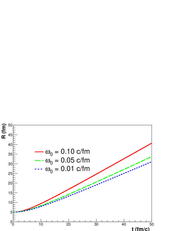
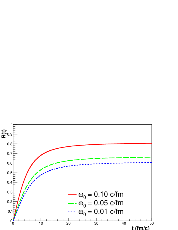
Figure 1: Time evolution of the axes $X(t)=Z(t)\equiv R(t)$ (upper panel) and the corresponding velocity, $\dot{R}(t)$ (lower panel) for our hydrodynamical model in three cases of $\omega_{0}$. Initial conditions are: $R_{0}=5$ fm, $Y_{0}=5$ fm, $\dot{R}=\dot{Y}=0$, $T_{0}=350$ MeV. One sees that increased initial angular momentum leads to increased, more violent explosion in the radial direction.

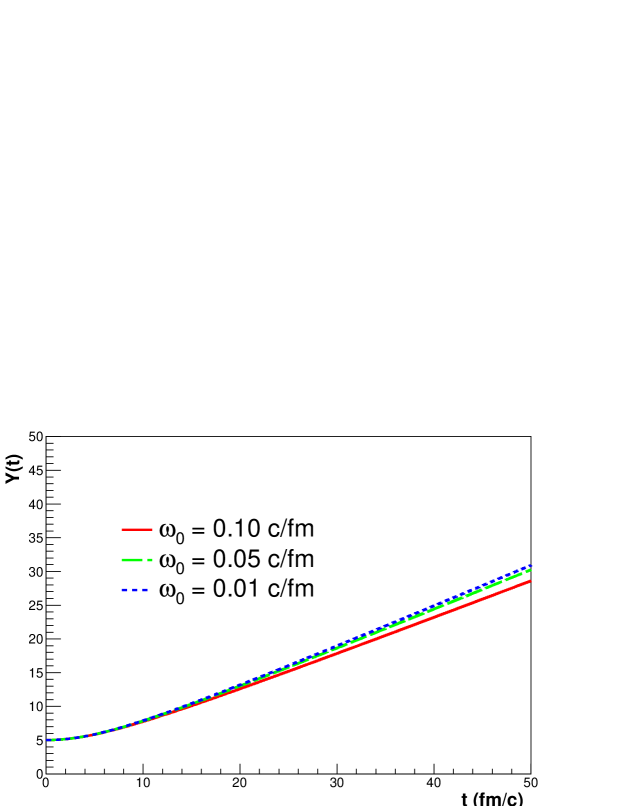
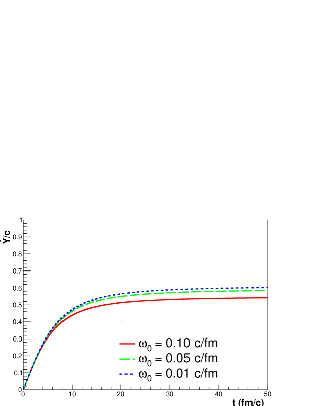
Figure 2: Time evolution of the $Y(t)$ axis (upper panel) and $\dot{Y}(t)$ (lower panel) for our hydrodynamical model in three cases of $\omega_{0}$. Initial conditions are the same as in Fig. 1. The more violent radial expansion related to increased values of initial angular momentum results in decreased expansion in the $Y$ direction, due to the faster cooling and the correspondingly faster decrease of the pressure of the fireball.

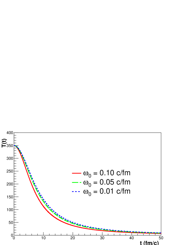
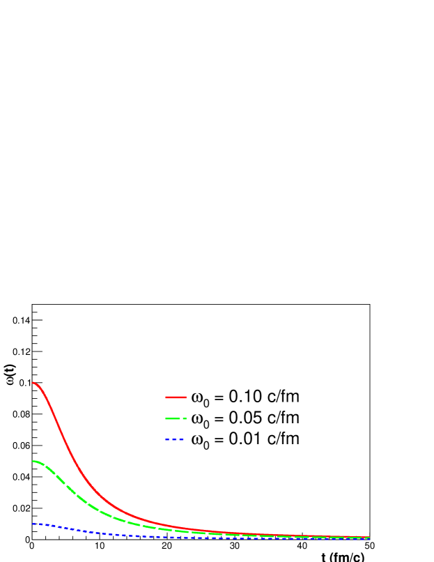
Figure 3: Time evolution of the temperature (upper panel) and the angular velocity (lower panel) for our hydrodynamical model in three cases of $\omega_{0}$. In this demonstrational case, $\kappa=3/2$, so the temperature is directly related to the geometrical size of the fireball through Eq. (15). Initial conditions are the same as in Fig. 1. Larger initial angular momentum leads to faster radial expansion, that causes faster cooling. In this class of rotating and expanding, spheroidal fireball solutons, the time evolution of the $r_{y}$ component of the vorticity vector, $\mathbf{\omega}_{y}(t)$ equals with twice the angular velocity $\omega(t)$ indicated on the lower panel, due to eq. (23).

In what follows, we demonstrate that the parameters $T_{x}$ and $T_{y}$ introduced in eqs. (20-22) in this manuscript play a very similar role to that of the analogous variables introduced in Ref. Csorgo:2001xm . There, the dynamics of the rotation was not taken into account, consequently the expressions of $T_{x}$ and $T_{y}$ lacked the term corresponding to the rotational energy, $R^{2}\omega^{2}$ (with $X=Z=R$), but these terms are clearly identified in the present manuscript. This way we prove, that in this class of rotating solutions of fireball hydrodynamics the effect of rotation enters the final state in a rather straightforward way: the effects that were usually associated with that of radial flows need to be re-considered to take the rotation effects also into account.

The presence of rotation changes the time evolution of the system and thus for a given initial condition, it influences the final state in an involved way. It is thus rather reassuring to find the simple forms of the rotational terms in the expression of the effective temperatures $T_{x}=T_{z}$ and $T_{y}$, as a manifestation of rotation.

III.1 Single particle spectrum

The single-particle spectrum is basically the integral of $S(\mathbf{r},\mathbf{p})$ over the spatial coordinates. The result is

$$E\frac{dn}{d^{3}\mathbf{p}} \propto E\exp\left\{{-\frac{p_{x}^{2}}{2mT_{x}}-\frac{p_{y}^{2}}{2mT_{y}}-\frac{p_{z}^{2}}{2mT_{z}}}\right\}.$$ (25)

Here $E$ is the energy of the particle. In our case, $T_{x}=T_{z}$, since $X_{f}=Z_{f}$. In this case the spectrum is rotationally invariant in the $x$–$z$ plane, so the observables calculated in this way are automatically valid in the laboratory frame as well as the rotated frame of the fluid. However, in the more general, yet to be explored case of a rotating and expanding ellipsoid with three different axes, this statement is generally not true: in that case, the observables calculated in the rest frame of the collision will differ from those measured in the proper frame of the ellipsoid at freeze-out.

The spectrum seen in Eq. (25) generates the following azimuthally averaged single-particle spectrum ($p_{t}$ stands for transverse momentum):

$$\frac{dn}{2\pi p_{t}dp_{t}dp_{z}} \propto \exp\left(-\frac{p_{t}^{2}}{2mT_{\rm eff}}-\frac{p_{z}^{2}}{2mT_{z}}\right)I_{0}(w),$$ (26)

$$\frac{1}{T_{\rm eff}} = \frac{1}{2}\left({\frac{1}{T_{x}}+\frac{1}{T_{y}}}\right),$$ (27)

$$w = \frac{p_{t}^{2}}{4m}\left({\frac{1}{T_{y}}-\frac{1}{T_{x}}}\right).$$ (28)

Here and in what follows, the modified Bessel function of order $n$ is denoted by $I_{n}\left({w}\right)$, which is defined as $I_{n}(w)=\frac{1}{\pi}\int_{0}^{\pi}\mathrm{d}z\cos(nz)\exp\left[{w\cos(z)}\right]$.

Just as we did for the time evolution of the system itself (see Figs. 1–3), we demonstrate the observables in the illustrative $X_{0}=Y_{0}=Z_{0}=5$ fm, $\dot{X}_{0}=\dot{Y}_{0}=\dot{Z}_{0}=0$, and $T_{0}=350$ MeV case, taken with three different values of initial angular velocity $\omega_{0}$, to display the effect of rotation on them.

In a relativistic generalization or extension, the mass dependence of the slope parameters transforms into the $m_{T}$ (transverse mass) dependence, see e.g. Refs. Csanad:2003qa ,Csorgo:1995bi , so our result on the $m$ dependence can be taken as a preliminary suggestion on the $m_{T}$ dependence what one might get in a more realistic relativistic approach. In our calculations, from now on we take the freeze-out temperature $T_{f}$ to be the pion mass, 140 MeV.

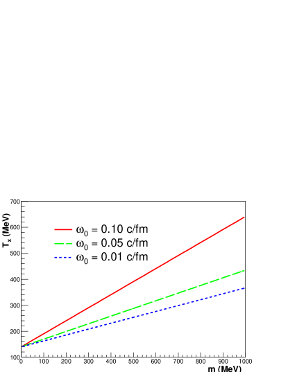
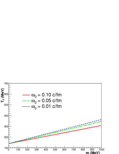
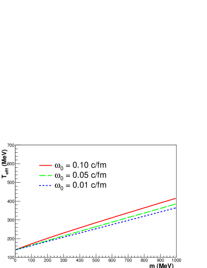
Figure 4: The slope parameters $T_{x}=T_{z}$ (upper panel), $T_{y}$ (middle panel) and the effective temperature introduced in Eq. (27), $T_{\rm eff}$ (lower panel), taken at freeze-out (when $T$ reaches $T_{f}=140$ MeV), as a function of particle mass $m$. As before, three cases of $\omega_{0}$ are selected for the purpose of demonstration of the analytically obtained formulas. Initial conditions are the same as in Fig. 1. Larger initial angular momentum creates additional terms that add to the radial flow effects, thus larger initial angular momentum leads to higher slope parameters or effective temperatures in the single particle spectrum..

The azimuthal dependence of the single-particle spectrum can be encoded in the Fourier components of it, these are called the flow coefficients, and denoted by $v_{n}$. They are defined as

$$\frac{dn}{dp_{z}p_{t}dp_{t}d\phi}=\frac{dn}{2\pi dp_{z}p_{t}dp_{t}}\left[1+2\sum_{n=1}^{\infty}v_{n}\cos(n\phi)\right].$$ (29)

Here $v_{1}$ is called the directed flow, $v_{2}$ the elliptic flow and $v_{3}$ the third flow. It is important to note that in our simple model all the event planes coincide and that is where we set the zero of the azimuthal angle, that’s why the sinusoidal terms do not appear in Eq. (29).

It turns out that in our model the transverse- and longitudinal momentum dependence of the $v_{n}$ flow components can be written in terms of the $w$ scaling variable introduced earlier in Eq. (27). Simple calculation leads now to

$$v_{2n+1}=0,\quad v_{2n}=\frac{I_{n}(w)}{I_{0}(w)}.$$ (30)

The odd components of the Fourier decomposition vanish. This is an artefact due to the spheroidal symmetry of the flow profile. In a more general case of non-spheroidal rotating expansion of an ellipsoid mentioned earlier, after Eq. (25), but not detailed in this manuscript, the observable angular tilt of the fireball would imply non-vanishing odd azimuthal moments. However, the even components mirror the effect of rotation as well: the $w$ variable, which governs the dependence of the flow components on the kinematic variables, and it increases compared to the non-rotating case of Ref. Csorgo:2001xm , corresponding to the increase of the elliptic flow due to the effect of rotation.

Figs. 5 and 6 illustrate again the case of the $X_{0}=Y_{0}=Z_{0}=5$ fm, $\dot{X}_{0}=\dot{Y}_{0}=\dot{Z}_{0}=0$, $T_{0}=350$ MeV initial conditions, with three different values of initial angular velocity $\omega_{0}$, to see how rotation influenced the evolution of the elliptic flow. In this particular case, we emphasize that the initial geometry is spherical, so elliptic flow develops as a dynamical effect entirely due to the angular momentum of an intially spherical volume. In a more realistic situation, where also initial geometrical asymmetries may be present, one thus expects that the elliptic flow also will be quite significantly influenced by the initial angular momentum of the participant zone.

Fig. 5 shows the values of $v_{2}$ for pions and protons (to display the effect of particle mass) taken at the freeze-out time, as a function of $p_{T}$, while Fig. 6 shows the $v_{2}$ of pions and protons for a representative $p_{T}$ value (300 MeV/c for pions, 1000 MeV/c for protons), as a function of freeze-out time. It is clear that in this demonstrative case of spherically symmetric initial conditions, rotation is what gives $v_{2}$ its magnitude. It is also straightforward then to conclude that the non-vanishing initial angular momentum of the participant zone may be an important contributor to the experimentally found and rather significant elliptic flow $v_{2}$ of observed particles.

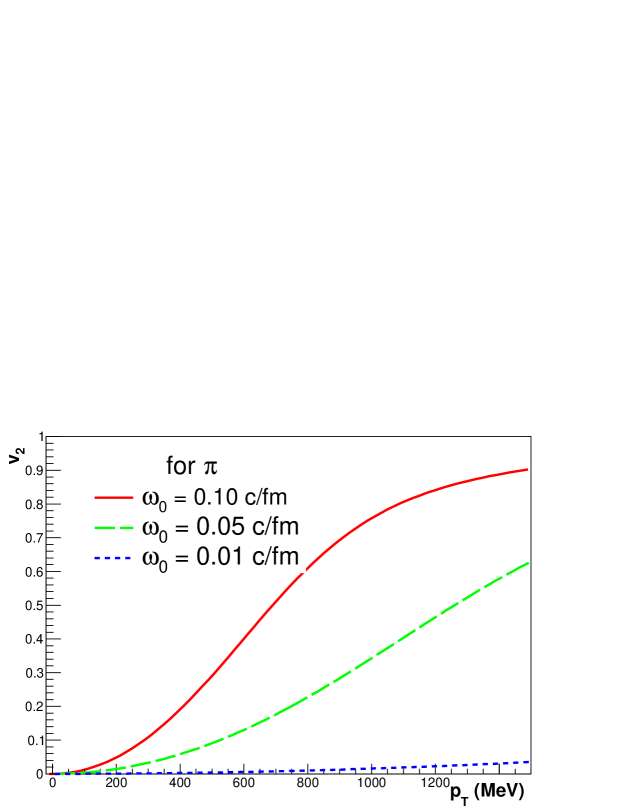
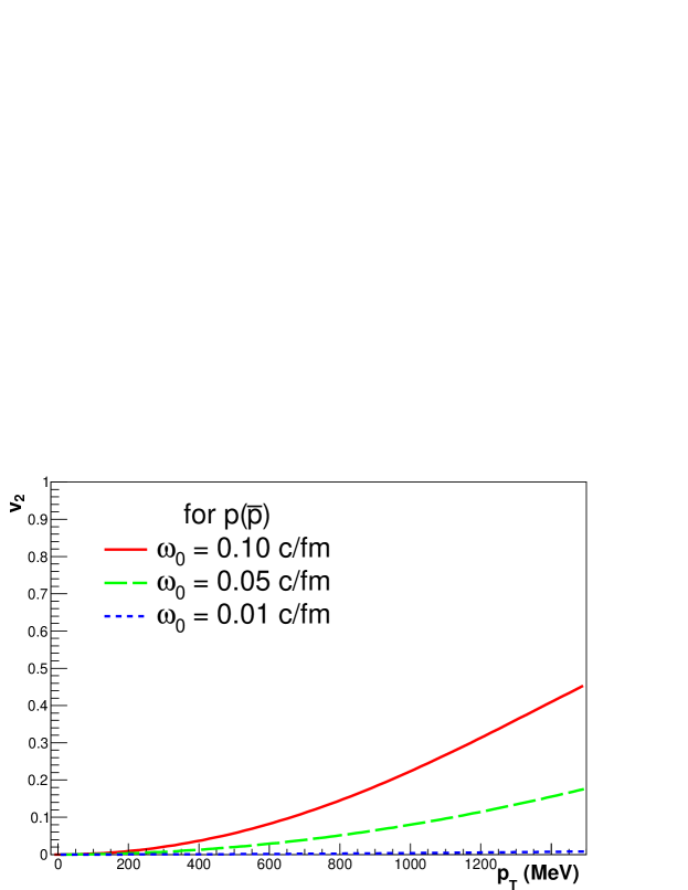
Figure 5: $v_{2}$ for pions (upper panel) and protons (lower panel) as a function of $p_{T}$ taken at the freeze-out time (when $T$ reaches $T_{f}=140$ MeV), for three different $\omega_{0}$ values. Initial conditions are the same as in Fig. 1. The effect of rotation is clearly the increase of the elliptic flow.

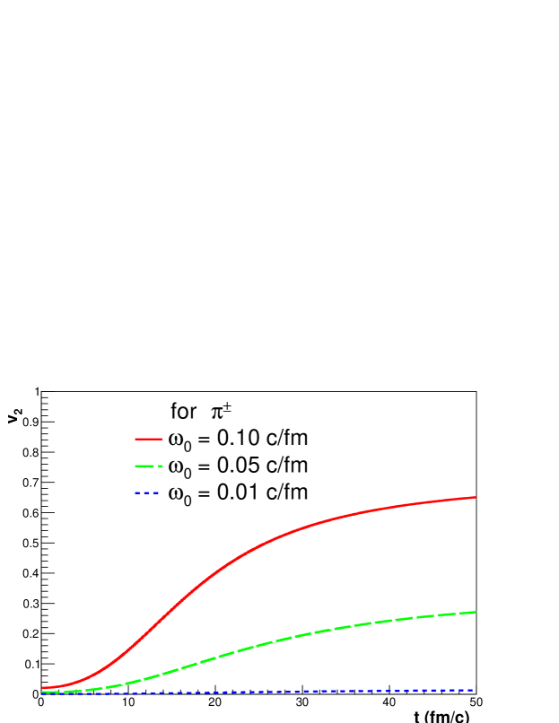
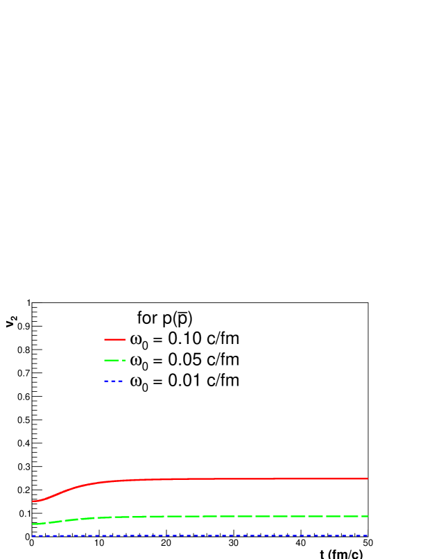
Figure 6: Freeze-out time dependence of $v_{2}$ for pions (upper panel) and protons (lower panel), at a fixed $p_{T}$ (300 MeV/c for pions and 1000 MeV/c for protons), for three different $\omega_{0}$ values. Initial conditions are the same as in Fig. 1. The effect of rotation is again seen to increase the elliptic flow.

III.2 Two-particle correlations

The two-particle Bose-Einstein correlation function (BECF) can be calculated from the Fourier-transform of the source function $S\left({t,\mathbf{r},\mathbf{p}}\right)$ of Eq. (19). For an introduction and review on this topic and the evaluation of Bose-Einstein correlation functions from analytic and realistic hydrodynamical models, we recommend Csorgo:1999sj . The simplest (spherically symmetric, nonrelativistic, non-rotational) examples for this kind of calculations are given in Refs. Csorgo:1994fg ; Csizmadia:1998ef , that we reproduce here in the special limit of zero initial angular momentum and spherical symmetry. Furthermore, utilizing the core-halo picture Csorgo:1994in one introduces the $\lambda$ parameter, the effective intercept of the correlation function: $\lambda\equiv\lambda\left({\mathbf{p}}\right)=\left[{N_{c}\left({\mathbf{p}}\right)/N\left({\mathbf{p}}\right)}\right]^{2}$. The $\lambda$ parameter measures the fraction of particles originating directly from the core, in contrast to those stemming from decay of longer lived resonances. The two-particle correlation function turns out to take the form

$$C\left({\mathbf{K},\mathbf{q}}\right) = 1+\lambda\exp\left\{{-q_{x}^{2}R_{x}^{2}-q_{y}^{2}R_{y}^{2}-q_{z}^{2}R_{z}^{2}}\right\},$$ (31)

$$\mathbf{K} = \mathbf{K}_{12}\,=\,\frac{1}{2}\left({\mathbf{p}_{1}+\mathbf{p}_{2}}\right),$$ (32)

$$\mathbf{q} = \mathbf{q}_{12}\,=\,\left({\mathbf{k}_{1}-\mathbf{k}_{2}}\right),$$ (33)

$$R_{x}^{2} = X_{f}^{2}\left({1+\frac{m}{T_{f}}\left({\dot{X}_{f}^{2}{+Z_{f}^{2}\omega_{f}^{2}}}\right)}\right)^{-1}\,=\,R_{f}^{2}\left({1+\frac{m}{T_{f}}\left({\dot{R}_{f}^{2}{+R_{f}^{2}\omega_{f}^{2}}}\right)}\right)^{-1},$$ (34)

$$R_{y}^{2} = Y_{f}^{2}\left({1+\frac{m}{T_{f}}\dot{Y}_{f}^{2}}\right)^{-1},$$ (35)

$$R_{z}^{2} = Z_{f}^{2}\left({1+\frac{m}{T_{f}}\left({\dot{Z}_{f}^{2}{+X_{f}^{2}\omega_{f}^{2}}}\right)}\right)^{-1}\,=\,R_{f}^{2}\left({1+\frac{m}{T_{f}}\left({\dot{R}_{f}^{2}{+R_{f}^{2}\omega_{f}^{2}}}\right)}\right)^{-1}.$$ (36)

Remember again, that although we have written these radius parameters in a symmetric way, the spheroidal symmetry of the applied solution, $X=Z$, $\dot{X}=\dot{Z}$, actually impies $R_{x}=R_{z}$. These radius parameters can also be called the lengths of homogeneity Sinyukov:1994vg . Again, note the very simple occurrence of rotational terms in the expression of the radius parameters, just as it was for the slope parameters $T_{x}=T_{z}$ and $T_{y}$ in Eqs. (20) and (22). These terms imply that increased initial angular momentum leads to an enhanced mass dependence and a decrease in the HBT radius parameters. This analytic result yields a deep insight into the earlier, numerically obtained indication that an increased rotation leads to a decreased HBT radius parameter, Ref. Velle:2015dpa .

Up to now we have dealt only with the case when the particle emission happens instantaneously (the delta function in Eq. (19) assures this). For Bose-Einstein correlations, it is instructive to see what happens when the freeze-out has a small but finite duration time. Let this duration be denoted by $\Delta t$. We evaluate the correlation functions by setting the time dependence of the source function equal to $(2\pi\Delta t^{2})^{-1/2}\exp[-(t-t_{f})^{2}/2\Delta t^{2}]$, instead of $\delta(t-t_{f})$. Performing the calculation again, one arrives at the conclusion that all the previous radius components, including the cross-terms, are supplemented with an additional term $\delta R^{2}_{ij}=\beta_{i}\beta_{j}\Delta t^{2}$, where $\mbox{\boldmath$\beta$}=({{\bf p}_{1}+{\bf p}_{2}})/({E_{1}+E_{2}})$ is the velocity of the pair.

We write up the Bose-Einstein correlation functions in a more usual parametrization, the so-called side-out-longitudinal or Bertsch-Pratt (BP) parameterization. In this parametrization, the longitudinal direction, $r_{\rm long}\equiv r_{\rm l}$ coincides with the beam direction, the . The ,,out” direction, $r_{{\rm out}}\equiv r_{\rm o}\,$ is parallel to the mean transverse momentum of the pair in the longitudinal co-moving frame (LCMS), and the side direction, $r_{\rm side}=r_{\rm s}\,$ is orthogonal to both of these. The mean velocity of the particle pair can be written in the Bertsch-Pratt system as $\mbox{\boldmath$\beta$}=(\beta_{\rm o},0,\beta_{\rm l})$, where $\beta_{\rm o}=\beta_{t}\,$. We denote by $\phi$ the angle of the event plane and the mean transverse momentum of the measured pair. Performing the coordinate transformation we obtain the following result:

$$C_{2}\left({\mathbf{K},\mathbf{q}}\right) = 1+\lambda\exp\left({-\sum_{i,j={\rm s,o,l}}q_{i}q_{j}R_{ij}^{2}}\right),$$ (37)

$$R^{2}_{\rm s} = R_{y}^{2}\cos^{2}\phi+R_{x}^{2}\sin^{2}\phi\,,$$ (38)

$$R^{2}_{\rm o} = R_{x}^{2}\cos^{2}\phi+R_{y}^{2}\sin^{2}\phi+\beta_{t}^{2}\Delta t^{2},$$ (39)

$$R^{2}_{\rm l} = R_{x}^{2}+\beta_{\rm l}^{2}\Delta t^{2},$$ (40)

$$R^{2}_{\rm ol} = \beta_{t}\beta_{\rm l}\Delta t^{2},$$ (41)

$$R^{2}_{\rm os} = \left({R_{x}^{2}-R_{y}^{2}}\right)\cos\phi\sin\phi\,,$$ (42)

$$R^{2}_{\rm sl} = {0}.$$ (43)

These results are simple and straightforward generalizations of the spheroidally symmetric special case of Ref. Csorgo:2001xm . As a function of $\phi$, many of these radius parameters oscillate. Again, it is important to emphasize that the fact that eg. $R_{\rm sl}=0$, and that $R_{\rm ol}=0$ for $\Delta t=0$, is not some general result, but rather an artefact of our considered class of spheroidal solutions where $X=Z$. In a more general case of $X\neq Z$, these cross-terms would appear (as seen eg. from the results for a non-rotating but tilted ellipsoid in Ref. Csorgo:2001xm .) The effect of rotation, however, enters in a very simple way: it results in the decrease of the radius parameters compared to the non-rotating case, as follows analytically from Eqs.  (34-36) that are related the observable HBT radii through Eqs. (38-43).

It is necessary to note that in the non-relativistic model investigated in this work, we see that the HBT radius parameters do not depend on the transverse momentum of the particle pair at all. To properly account for the observed $m_{T}$ dependence of the radius parameters, one needs to invoke relativistic dynamics; for example, in the Buda-Lund parametrizations of Refs.  Csanad:2003qa ,Csorgo:1995bi it turns out that the functional form of the dependence on particle mass $m$ seen in Eqs. (38)–(43) is approximately conserved, just in the relativistic case, the dependence is on the transverse mass $m_{T}$ of the particle pair. These parameterizations evolved to various hydrodynamical solutions, in particular the present manuscript can be considered as a non-relativistic, rotating and spheroidally symmetric Buda-Lund hydrodynamical solution. So, similarly to the remarks after Eq. (27), we conclude that as long as no relativistic description of the observables in a rotating system is available, our results give a hint at the proper dependence of the radius parameters on the kinematical variables by setting $m\to m_{T}$ in the formulas above.

As before, we illustrate the effects of rotation on the HBT radius parameters by taking a spherically symmetric initial condition with three different values of initial angular velocity. Fig. 7 shows the azimuthal angle dependence of $R^{2}_{\rm o}$, $R^{2}_{\rm s}$, and $R^{2}_{\rm os}$ at the freeze-out time, while Fig. 8 shows the dependence of the azimuthal mean value of $R^{2}_{\rm o}$ and $R^{2}_{\rm l}$ on the freeze-out time. (We plot only these ones, as the others are either not interesting or just very similar to these.) It is clearly seen that the overall magnitude of the azimuthal mean of the radius parameters decrease with rotation, as mentioned above. One also observes that all the oscillations become stronger with more rotation, a straightforward effect of anisotropic geometry stemming from the centrifugal force. This behavior is thus expected to be a general consequence of rotation.

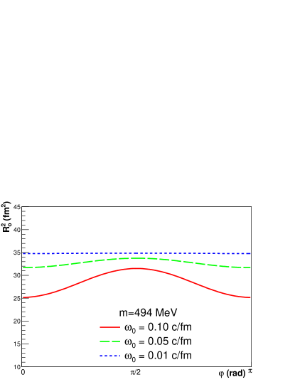
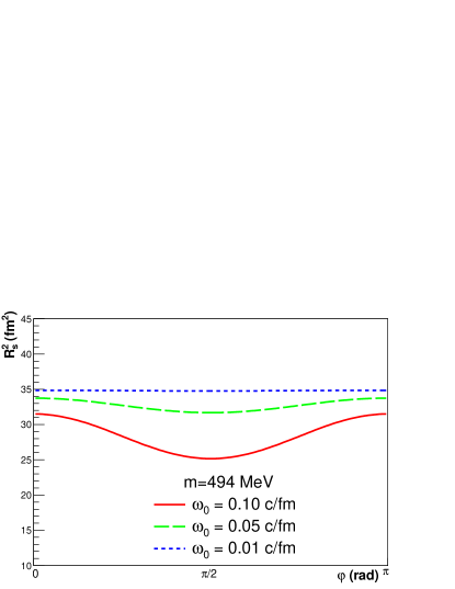
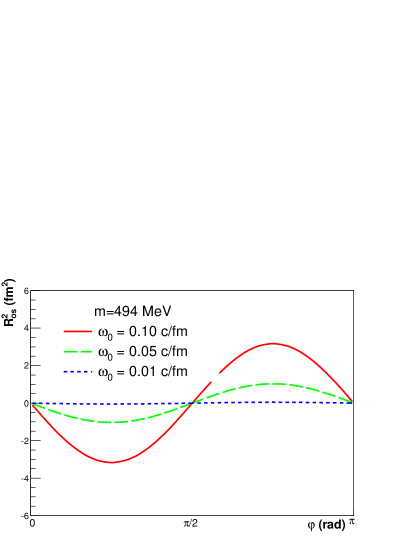
Figure 7: HBT radius parameters $R^{2}_{\rm o}$ (upper panel), $R^{2}_{\rm s}$ (middle panel) and the cross-term $R^{2}_{\rm os}$ (lower panel) as a function of the azimuthal angle of the pair, at freeze-out. Initial conditions are the same as in Fig. 1, but this observable was calculated for charged kaons, with mass $m=494$ MeV. The cases with three different $\omega_{0}$ values illustrate the effect of rotation: it causes more anisotropy as well as an overall decrease of the magnitude of the azimuthally averaged radii.

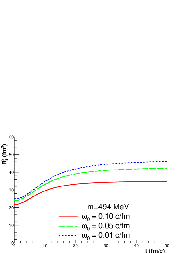
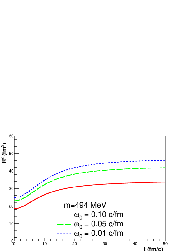
Figure 8: Freeze-out time dependence of the azimuthal average of $R^{2}_{\rm s}$ (upper panel) and $R^{2}_{\rm l}$ (lower panel). Initial conditions are the same as in Fig. 1, and three different $\omega_{0}$ values. but this observable was calculated for charged kaons, with mass $m=494$ MeV. Rotation decreases the magnitude of the radii.

IV Summary

We have evaluated the single-particle spectra, the elliptic and higher order flows, and the two-particle Bose-Einstein correlation functions for a rotating and expanding, spheroidally symmetric fireball, a non-relativistic Buda-Lund type hydrodynamical model.

A non-vanishing value of the initial angular momentum, an important conserved quantity that is characteristic to the non-central heavy ion collisions, was taken into account and its effects on the observables have been found using simple and straight-forward analytic formulae.

Although the hydrodynamical solution we used is non-relativistic, the insight it gives the observables in rotating systems is valuable and relevant for analyzing experimental measurements of the treated observables.

We have proven that rotational terms appear in the observables in a way that is rather similar to radial flow effects and lead to the increased mass dependence of the effective temperatures or slope parameters of the single particle spectra, an enhanced elliptic flow and a stronger mass-dependence of the decrease of the Bose-Einstein correlation radii. We have illustrated these analytic results with several plots utilizing an academic, but rather interesting spherical initial condition and initial angular velocities gradually increasing from a nearly vanishing value to a realistic value.

Using this special initial condition of a rotating and initially spherical fireball, have demonstrated that initial angular momentum leads to a significant elliptic flow even for the case when there are no initial spatial asymmetries present. This implies that future experimental data analysis has to take possible rotational effects into account as they may mix in a subtle and difficult to identify manner with other, more generally considered radial flow effects.

We also emphasize that to consider these important angular momentum and rotational effects, finite 3d hydrodynamical solutions have to be utilized for the data analysis, as infinite systems have infinite moments of intertia so they cannot realistically model rotating hydrodynamical solutions.

Appendix A Equations of motion for $\kappa=3/2$

For $\kappa=3/2$, the solution of the equations of motion, Eq. (11) can be given using the Hamilton-Jacobi formalism, applied to the (16) Hamiltonian. This formalism can be applied for a classical Hamiltonian $H\left({P_{i},Q_{i},t}\right)$ as follows. (Here $P_{i}$ and $Q_{i}$ denote the $N$ canonical momenta and coordinates.) One must find the classical Hamilton function, or action $S\left({Q_{i},t}\right)$ that is a solution of the Hamilton-Jacobi equation:

$$\frac{\partial S}{\partial t}+H\left({\frac{\partial S}{\partial Q_{i}},Q_{i},t}\right)=0.$$

If a suitable solution $S\left({Q_{i},t,K_{i}}\right)$ is found, which has $N$ different arbitary parameters $K_{i}$, then the equations $\frac{\partial}{\partial K_{i}}S\left({Q_{i},t,K_{i}}\right)=L_{i}$, again with arbitary constants $L_{i}$, give the solution of the equation of motion.

In cases where $H$ is time-dependent, the conserved energy $E$ enters as a free parameter:

$$S\left({Q_{i},t}\right)=-Et+S\left({Q_{i}}\right),\quad H\left({\frac{\partial S(Q_{i})}{\partial Q_{i}},Q_{i}}\right)=E.$$

In our case, for $\kappa=3/2$, we have

$$\frac{\left({\frac{\partial S}{\partial R}}\right)^{2}+2\left({\frac{\partial S}{\partial Y}}\right)^{2}}{4m}+\frac{m\omega_{0}^{2}R_{0}^{4}}{R^{2}}+\frac{3T_{0}}{2}\left({\frac{R_{0}^{2}Y_{0}}{R^{2}Y}}\right)^{\frac{2}{3}}=E.$$

This can be solved by introducing the $\rho$, $\chi$ variables (like planar cylindrical coordinates) as

$$R=\frac{\rho}{\sqrt{2}}\cos\chi,\quad Y=\rho\sin\chi,$$

and re-arranging the Hamilton-Jacobi equation to obtain

$$\left({\frac{\partial S}{\partial\rho}}\right)^{2}+\frac{1}{\rho^{2}}\left\{{\left({\frac{\partial S}{\partial\chi}}\right)^{2}+F\left({\chi}\right)}\right\}=2mE,$$

with

$$F\left({\chi}\right)=2m^{2}\omega_{0}^{2}R_{0}^{4}+3mT_{0}\left({\frac{2R_{0}^{2}Y_{0}}{\cos^{2}\chi\sin\chi}}\right)^{2/3}.$$

The desired solution is now obtained straightforwardly, by introducing the $K$ constant so that the equation becomes separable. We thus can assume that $S\left({\rho,\chi}\right)=S_{1}\left({\rho}\right)+S_{2}\left({\chi}\right)$, and get the following solution:

$$\left({\frac{\partial S_{1}}{\partial\rho}}\right)^{2}+\frac{K}{\rho^{2}}=2mE,\quad\left({\frac{\partial S_{2}}{\partial\chi}}\right)^{2}+F\left({\chi}\right)=K\quad\Rightarrow$$

$$S=-Et+\int\mathrm{d}\rho\sqrt{2mE-\frac{K}{\rho^{2}}}+\int\mathrm{d}\chi\sqrt{K-F\left({\chi}\right)}.$$

The equations of motion now can be considered as solved. Taking the $\frac{\partial S}{\partial E}=B_{1}=$const condition, with elementary integration we get the following result:

$$\rho^{2}=\frac{2E}{m}\left({t+B_{1}}\right)^{2}+\frac{K}{2mE}.$$ (44)

If one writes back $R$ and $Y$ in this result, and chooses the $K$ and $B_{1}$ constants to match the initial conditions, one gets the following:

$$2R^{2}+Y^{2}=\frac{2E}{m}t^{2}+\left({4\dot{R}_{0}R_{0}+2\dot{Y}_{0}Y_{0}}\right)t+2R_{0}^{2}+Y_{0}^{2},$$ (45)

where the $E$ energy is in this case

$$\frac{E}{m}=\dot{R}_{0}^{2}+\frac{\dot{Y}_{0}^{2}}{2}+\omega_{0}^{2}R_{0}^{2}+\frac{3T_{0}}{2m}.$$

Substituting $E$ back in Eq. (45), one readily arrives at Eq. (18). This gives the time dependence of $2R^{2}+Y^{2}$. This result could have been inferred by simple inspection of the differential equations, and once this is known, a univariate differential equation also can be given (and numerically solved) for the remaining independent variables. This was known already in Ref Akkelin:2000ex (although not for a rotating system). Our method here gives the solution by quadratures: it is easy to see that the other condition coming from the Hamilton-Jacobi method, $\frac{\partial S}{\partial K}=B_{2}=$const, does not contain the time variable $t$. So this condition fixes the shape of the trajectory in the $R$–$Y$ ,,plane”. However, in general it cannot be evaluated analytically.

Appendix B A survey of analytic solutions

In this Appendix we give a short list of some recent exact analytic solutions of the non-relativistic hydrodynamical equations. We do this in the hope that just as uniting efforts in heavy-ion physics and analytical hydrodynamics has been proven to be of much interest for both research directions, it can and will prove fruitful also in future applications (even though the heavy-ion physical applications of the mentioned solutions is not clear yet).

In spite of the lacking basic mathematical theorems (like existence and uniqueness) there is a fairly great amount of analytic solutions available for various hydrodynamical equations like the Euler or the Navier-Stokes(NS) equations. high-energy physics we give a short overview about the recent developments in analytical hydrodynamics.

There are various examination techniques available with numerous studies in the literature. Most of them are based on the application of the self-similar Ansatz or on Lie algebra methods.

Sedov in his classical work about self-similar solutions sedov presents one of the first analytic solutions for the three dimensional spherical NS equation where all three velocity components and the pressure have polar angle dependence ($\theta$) only. Some similarity reduction solutions of the two dimensional incompressible NS equation was presented by Xia-Yu jiao . Additional solutions are available for the 2+1 dimensional NS also via symmetry reduction techniques by fakhar . Manwai manwai studied the N-dimensional $(N\geq 1)$ radial Navier-Stokes equation with different kind of viscosity and pressure dependences and presented analytical blow up solutions. His works are still 1+1 dimensional (one spatial and one time dimension) investigations.

In our former study we generalized the self-similar Ansatz of Sedov and presented analytic solutions for the most general three dimensional Navier-Stokes equation in Cartesian coordinates imre . The solutions are the Kummer functions with quadratic arguments. Later, we applied our method to the three dimensional compressible NS equation where the politropic equation of state was used imre2 resulting in the Whitakker functions.

Recently, Hu et al. hu presented a study where symmetry reductions and exact solutions of the (2+1)-dimensional NS were presented. Aristov and Polyanin arist use various methods like Crocco transformation, generalized separation of variables or the method of functional separation of variables for the NS and present large number of new classes of exact solutions.

A universal Lie algebra study is available for the most general three dimensional NS lie . Unfortunately, no explicit solutions are shown and analyzed there. Fushchich et al. fus constructed a complete set of ${\tilde{G}}(1,3)$-inequivalent Ansätze of codimension one for the NS system, they present 19 different analytical solutions for one or two space dimensions. Further, two and three dimensional studies based on group theoretical method were presented by Grassi grassi getting Whitakker functions for solutions which are very similar to our results mentioned earlier imre .

References

- (1) L. P. Csernai, V. K. Magas, H. Stocker and D. D. Strottman, Phys. Rev. C 84, 024914 (2011) [arXiv:1101.3451 [nucl-th]].
- (2) L. Cifarelli, L. P. Csernai and H. Stocker, Europhys. News 43, no. 2, 29 (2012).
- (3) L. P. Csernai, S. Velle and D. J. Wang, Phys. Rev. C 89, no. 3, 034916 (2014) [arXiv:1305.0396 [nucl-th]].
- (4) L. P. Csernai and S. Velle, arXiv:1305.0385 [nucl-th].
- (5) S. Velle and L. P. Csernai, Phys. Rev. C 92, no. 2, 024905 (2015) [arXiv:1508.01884 [nucl-th]].
- (6) S. Velle, S. M. Pari and L. P. Csernai, arXiv:1508.04017 [nucl-th].
- (7) T. Csörgő and M. I. Nagy, Phys. Rev. C 89, no. 4, 044901 (2014) [arXiv:1309.4390 [nucl-th]].
- (8) P. Csizmadia, T. Csörgő and B. Lukács, Phys. Lett. B 443, 21 (1998) [nucl-th/9805006].
- (9) M. I. Nagy, Phys. Rev. C 83, 054901 (2011) [arXiv:0909.4285 [nucl-th]].
- (10) Y. Hatta, J. Noronha and B. W. Xiao, Phys. Rev. D 89, no. 5, 051702 (2014) [arXiv:1401.6248 [hep-th]].
- (11) Y. Hatta, J. Noronha and B. W. Xiao, Phys. Rev. D 89, no. 11, 114011 (2014) [arXiv:1403.7693 [hep-th]].
- (12) B. McInnes, Nucl. Phys. B 887, 246 (2014) [arXiv:1403.3258 [hep-th]].
- (13) R. D. de Souza, T. Koide and T. Kodama, arXiv:1506.03863 [nucl-th].
- (14) Y. Xie, R. C. Glastad and L. P. Csernai, arXiv:1505.07221 [nucl-th].
- (15) F. Becattini, L. Csernai and D. J. Wang, Phys. Rev. C 88, no. 3, 034905 (2013) [arXiv:1304.4427 [nucl-th]].
- (16) L. P. Csernai and J. H. Inderhaug, Int. J. Mod. Phys. E 24, no. 02, 1550013 (2015) [arXiv:1503.03247 [nucl-th]].
- (17) L. P. Csernai, D. J. Wang and T. Csörgő, Phys. Rev. C 90, no. 2, 024901 (2014) [arXiv:1406.1017 [hep-ph]].
- (18) T. Csörgő, S. V. Akkelin, Y. Hama, B. Lukács and Y. M. Sinyukov, Phys. Rev. C 67, 034904 (2003) [hep-ph/0108067].
- (19) K. Adcox et al. [PHENIX Collaboration], Nucl. Phys. A 757, 184 (2005) [nucl-ex/0410003].
- (20) J. Adams et al. [STAR Collaboration], Nucl. Phys. A 757, 102 (2005) [nucl-ex/0501009].
- (21) F. Becattini, M. Bleicher, T. Kollegger, T. Schuster, J. Steinheimer and R. Stock, Phys. Rev. Lett. 111, 082302 (2013) [arXiv:1212.2431 [nucl-th]].
- (22) M. Csanád, T. Csörgő and B. Lörstad, Nucl. Phys. A 742, 80 (2004) [nucl-th/0310040].
- (23) T. Csörgő, Acta Phys. Polon. B 37, 483 (2006) [hep-ph/0111139].
- (24) S. V. Akkelin, T. Csörgő, B. Lukács, Y. M. Sinyukov and M. Weiner, Phys. Lett. B 505, 64 (2001) [hep-ph/0012127].
- (25) T. Csörgő, Heavy Ion Phys. 15, 1 (2002) [hep-ph/0001233].
- (26) T. Csörgő, B. Lörstad and J. Zimányi Phys. Lett. B 338, 134 (1994) [nucl-th/9408022].
- (27) T. Csörgő, B. Lörstad and J. Zimányi, Z. Phys. C 71, 491 (1996) [hep-ph/9411307].
- (28) T. Csörgő and B. Lörstad, Phys. Rev. C 54, 1390 (1996) [hep-ph/9509213].
- (29) Y. M. Sinyukov, Nucl. Phys. A 566, 589C (1994).
- (30) L. Sedov, Similarity and Dimensional Methods in Mechanics CRC Press 1993 * (Page 120).
- (31) J. Xia-Yu, Commun. Theor. Phys. 52 (2009) 389.
- (32) K. Fakhar, T. Hayat, C. Yi and N. Amin, Commun. Theor. Phys. 53 (2010) 575.
- (33) Y. Manwai, J. Math. Phys. 49 (2008) 113102.
- (34) I.F. Barna, Commun. Theor. Phys. 56 (2011) 745.
- (35) I.F. Barna and L. Mátyás, Fluid. Dyn. Res. 46 (2014) 055508.
- (36) X.R. Hu, Z.Z. Dong, F. Huang et al., Z. Naturforschung A 65 (2010) 504.
- (37) S. N. Aristov and A. D. Polyanin, Russ. J. Math. Phys. 17 (2010) 1.
- (38) V.N. Grebenev, M. Oberlack and A.N. Grishkov, Journ. of Nonlin. Mathem. Phys 15 (2008) 227.
- (39) W. I. Fushchich, W. M. Shtelen and S. L. Slavutsky J. Phys. A: Math. Gen. 24 (1990) 971.
- (40) V. Grassi, R.A. Leo, G. Soliani and P. Tempesta, Physica 286 (2000) 79 *, ibid 293 (2000) 421.