Simulating the galaxy cluster “El Gordo” and identifying the merger configuration

Abstract

The observational features of the massive galaxy cluster “El Gordo” (ACT-CL J0102–4915), such as the X-ray emission, the Sunyaev-Zel’dovich (SZ) effect, and the surface mass density distribution, indicate that they are caused by an exceptional ongoing high-speed collision of two galaxy clusters, similar to the well-known Bullet Cluster. We perform a series of hydrodynamical simulations to investigate the merging scenario and identify the initial conditions for the collision in ACT-CL J0102–4915. By surveying the parameter space of the various physical quantities that describe the two colliding clusters, including their total mass ($M$), mass ratio ($\xi$), gas fractions ($f_{\rm b}$), initial relative velocity ($V$), and impact parameter ($P$), we find out an off-axis merger with $P\sim 800\,h_{70}^{-1}{\rm\,kpc}$, $V\sim 2500{\rm\,km\,s^{-1}}$, $M\sim 3\times 10^{15}{\,M_{\odot}}$, and $\xi=3.6$ that can lead to most of the main observational features of ACT-CL J0102–4915. Those features include the morphology of the X-ray emission with a remarkable wake-like substructure trailing after the secondary cluster, the X-ray luminosity and the temperature distributions, and also the SZ temperature decrement. The initial relative velocity required for the merger is extremely high and rare compared to that inferred from currently available $\Lambda$ cold dark matter ($\Lambda$CDM) cosmological simulations, which raises a potential challenge to the $\Lambda$CDM model, in addition to the case of the Bullet Cluster.

1 Introduction

Clusters of galaxies are unique laboratories for exploring the nature of dark matter (DM) and the structure formation in the universe (see a recent review by Kravtsov & Borgani, 2012). In the $\Lambda$ cold dark matter ($\Lambda$CDM) cosmology, massive galaxy clusters are assembled via accretion and mergers of galaxy groups or small clusters. Some clusters are undergoing mergers and dynamically unrelaxed systems with distinctive features, which are expected to provide deep insights not only into the merging process but also into the physics of hierarchical structure formation. For example, studies of the Bullet Cluster (1E 0657–56; e.g., Markevitch et al. 2002) have demonstrated almost exclusively the collisionless nature of DM (Clowe et al., 2004; Clowe et al., 2006; Milosavljević et al., 2007; Springel & Farrar, 2007; Mastropietro & Burkert, 2008), and also revealed that the relative velocity ($\sim 2700-4500{\rm\,km\,s^{-1}}$) required for the merger to form the Bullet Cluster may be too high and rare to be compatible with the prediction from the $\Lambda$CDM model and thus put a strong constraint on the model (e.g., Lee & Komatsu, 2010; Thompson & Nagamine, 2012; Bouillot et al., 2014, but see Watson et al. 2014; Thompson et al. 2015; Lage & Farrar 2015; Kraljic & Sarkar 2015).

ACT-CL J0102–4915 (“El Gordo”), a Bullet Cluster-like cluster at a redshift of $z=0.87$, was recently discovered by the Atacama Cosmology Telescope (ACT) through its Sunyaev-Zel’dovich (SZ) effect (Marriage et al., 2011). ACT-CL J0102–4915 was also detected by the South Pole Telescope (SPT) and Planck SZ surveys (Williamson et al., 2011; Planck Collaboration et al., 2014). Multi-frequency observational follow-ups, including those in the optical, X-ray, infrared, and radio bands, have shown that ACT-CL J0102–4915 is a rare and exceptional system (Menanteau et al., 2012; Jee et al., 2014; Lindner et al., 2014) at least in the following points. (1) It is the most massive X-ray and SZ bright cluster ($\sim 2-3\times 10^{15}\,h_{70}^{-1}{\,M_{\odot}}$) at $z\gtrsim 0.6$ discovered so far. (2) The offsets between its SZ and X-ray centroids ($\sim 600\,h_{70}^{-1}{\rm\,kpc}$) and between its SZ centroid and the mass center of its main cluster component ($\sim 150\,h_{70}^{-1}{\rm\,kpc}$) are quite large. (3) The morphology of its X-ray emission is elongated with two extended faint tails, possibly a “wake”-like feature. (4) It is currently the highest-redshift cluster that hosts a radio relic. These observational features suggest that ACT-CL J0102–4915 is probably undergoing a major merger with high relative velocity ($V\sim 1200-2300$, $2600$, or $2250{\rm\,km\,s^{-1}}$ obtained in Menanteau et al. 2012, Donnert 2014, or Molnar & Broadhurst 2015, respectively). However, the probability is extremely low for the existence of a massive major merger with such a high initial relative velocity in the currently available large-volume cosmological simulations (Menanteau et al. 2012; see also Jee et al. 2014), which raises a potential challenge to the $\rm\Lambda CDM$ model, in addition to the case of the Bullet Cluster.

To understand those distinctive observational features of ACT-CL J0102–4915, it is important and necessary to investigate its detailed merging behavior by performing $N$-body/hydro-numerical simulations and reproducing the observations, which may further help to constrain the $\rm\Lambda CDM$ model.

In this work, we perform a series of numerical simulations of mergers of two massive clusters and find out the merger configurations that can lead to a good match to various observations of ACT-CL J0102–4915. Some simulations on collisions between two isolated clusters have been carried out previously to investigate the nature of some particular clusters (e.g., the Bullet Cluster; see Springel & Farrar, 2007; Mastropietro & Burkert, 2008; ZuHone et al., 2009; Machado & Lima Neto, 2013). For example, Molnar & Broadhurst (2015) have simulated cluster mergers by using the FLASH code (Fryxell et al., 2000) to reproduce the observations of ACT-CL J0102–4915 (see also Donnert 2014). They found that the two extended faint X-ray tails of ACT-CL J0102–4915 may be reproduced through a nearly head-on merger of two massive clusters, however, where only nine sets of initial conditions of the merging configurations are explored. Considering both the advantages and the disadvantages in different kinds of hydrodynamical simulations, in this work we first perform a large number of merger simulations ($\sim 120$) by using the efficient GADGET-2 code. We survey the parameter space and find out the configuration of those mergers that can lead to a good match to various observations of ACT-CL J0102–4915. Then we further resimulate those mergers by using the FLASH code, with which some substructures (shocks, eddies, etc.) can be more accurately simulated.

The paper is organized as follows. In Section 2, we describe the method of simulating cluster mergers and generating the mock observational maps. We present our simulation results in Section 3. Two types of the simulated merging systems (i.e., the nearly head-on merger and the highly off-axis merger) are explored. Detailed comparison of the simulation results with the observational ones is also presented in this section. We further discuss the effects of the gas fraction profile of galaxy clusters on simulating the “El Gordo”. Conclusions are summarized in Section 4.

Throughout the paper, we assume a flat $\rm\Lambda CDM$ cosmology model with $\Omega_{\rm m}=0.30$, $\Omega_{\rm\Lambda}=0.70$, and the Hubble constant $H_{0}=70\,h_{70}{\rm\,km\,s^{-1}}{\rm\,Mpc}^{-1}$.

2 Method

We simulate the mergers of galaxy clusters by adopting the two types of publicly available numerical codes: (1) the GADGET-2 code (Springel et al., 2001) and (2) the FLASH code (Fryxell et al., 2000; Ricker, 2008). The GADGET-2 code uses the smoothed particle hydrodynamics (SPH) method to solve the gas hydrodynamics, and it has advantages in computational speed and effective resolution (Springel et al., 2001). However, it may not handle shocks, eddies, and fluid instabilities accurately (Mitchell et al., 2009; Agertz et al., 2007). The FLASH code uses the piecewise-parabolic method (PPM; Colella & Woodward 1984) to solve the gas hydrodynamics and the adaptive mesh refinement (AMR) method to reach high spatial resolution only where it is needed. The FLASH code handles shocks, eddies and fluid instabilities better than the SPH code, but it is time-consuming.

Considering the advantages of the GADGET-2 code in computational speed (generally about one order of magnitude faster than the FLASH code for the mergers with the same initial conditions in our simulations), we first use the GADGET-2 code to survey the parameter space for the initial conditions and configurations of cluster mergers and search for the one that can “best fit” the observations of ACT-CL J0102–4915 (denoted as the fiducial model(s)). The mass resolutions of DM and baryonic gas are set to be $1.65\times 10^{9}\,h_{70}^{-1}{\,M_{\odot}}$ and $1.68\times 10^{8}\,h_{70}^{-1}{\,M_{\odot}}$, respectively. We resimulate the fiducial models (see Sections 3.1 and 3.2) by using the FLASH code, which offers a better treatment to the fine structures of the merging cluster. The box size of our simulations is $15.6\,h_{70}^{-1}{\rm\,Mpc}$ on each side, and the finest resolution achieved is $7.6\,h_{70}^{-1}{\rm\,kpc}$. In our simulations, the two progenitor clusters of ACT-CL J0102–4915 are assumed to be spherical halos, composed of collisionless DM and adiabatic collisional gas; the shock heating is included, while the radiative cooling and additive heating mechanisms (e.g., active galactic nucleus (AGN) feedback) are neglected.

The setup of the initial configuration of the merging cluster and the method to analyze the simulation data are introduced in Sections 2.1 and 2.2 below, respectively.

2.1 Initial Configuration

Considering a merger of two clusters, the masses of the primary and the secondary clusters are denoted as $M_{1}$ and $M_{2}$ ($M_{1}\geq M_{2}$), respectively, and the mass ratio is $\xi\equiv M_{1}/M_{2}$. Within the radius $r_{\rm 200}$, the fractions of the baryon mass to the total mass are denoted as $f_{\rm b1}$ and $f_{\rm b2}$ for the primary and the secondary clusters, respectively. A Cartesian coordinate system $x^{\prime}y^{\prime}z^{\prime}$ is adopted for our simulations. The collision of those two clusters is assumed to occur in the $x^{\prime}-y^{\prime}$ plane. The initial positions of the cluster centers are set to be $(d_{\rm ini}/(1+\xi),\ P/(1+\xi),\ 0)$ and $(-d_{\rm ini}\xi/(1+\xi),\ -P\xi/(1+\xi),\ 0)$, respectively, where $P$ is the impact parameter, and $d_{\rm ini}$ is twice the sum of the radii $r_{200}$ of the two clusters. The initial separation between the two clusters is $\sqrt{d^{2}_{\rm ini}+P^{2}}\sim d_{\rm ini}$ as $d_{\rm ini}\gg P$ for most cases studied in this work. The initial velocities of the primary and the secondary clusters are set to be $(-V/(1+\xi),\ 0,\ 0)$ and $(V\xi/(1+\xi),\ 0,\ 0)$, respectively, with which the mass center of the merging system maintains at rest at the origin, and $V$ is the initial relative velocity.

For each cluster, we assume that the DM density distribution follows the Navarro-Frenk-White (NFW; Navarro et al. 1997) profile within $r_{\rm 200}$, i.e.,

$$\rho_{\rm DM}(r)=\frac{\rho_{\rm s}}{r/r_{\rm s}(1+r/r_{\rm s})^{2}},\quad{\rm for\ }r\leq r_{\rm 200},$$ (1)

where $\rho_{\rm s}$ and $r_{\rm s}\equiv r_{\rm 200}/c_{\rm 200}$ are the scale density and radius, and $c_{\rm 200}$ is the concentration parameter. For a cluster with a given mass, $c_{\rm 200}$ can be obtained by using the mass-concentration relation of Duffy et al. (2008); and in this work we adopt the median of the statistical relationship (see table 1 in Duffy et al. 2008). We assume an exponential truncation of the DM density distribution outside $r_{\rm 200}$ to avoid a divergent total mass. More details can be found in Kazantzidis et al. (2004). The velocities of DM particles are assigned according to the distribution function derived from the Eddington’s formula (eq. 4.46 in Binney & Tremaine 2008).

The gas density distribution is assumed to follow the Burkert profile (Burkert, 1995),

$$\rho_{\rm gas}(r)=\frac{\rho_{\rm c}}{(1+(r/r_{\rm c})^{2})(1+r/r_{\rm c})},\quad{\rm for\ }r\leq r_{\rm 200},$$ (2)

where $r_{\rm c}$ is the core radius, which is typically half of $r_{\rm s}$ (Ricker & Sarazin, 2001). The gas density profile outside of $r_{\rm 200}$ is assumed to trace the density distribution of DM (see eq. 4 in Zhang et al. 2014). We set $r_{\rm c}=r_{\rm s}/2$ for the primary cluster. For the secondary cluster, we find that a smaller $r_{\rm c}$ would provide a better fit to the observational X-ray morphology according to our simulations. Therefore, we choose $r_{\rm c}=r_{\rm s}/3$ for the secondary cluster. The normalization factor $\rho_{\rm c}$ can be obtained by equating the baryon mass fraction within $r_{\rm 200}$ to $f_{\rm b1}$ and $f_{\rm b2}$ for the primary and secondary cluster, respectively. Assuming that the gas is in hydrostatic equilibrium and ideal (with a heat capacity ratio of $\gamma=5/3$), the temperature and the specific internal energy distribution of the gas in each progenitor cluster can all be numerically determined (Ricker & Sarazin, 2001). The effects of different gas density profiles are further discussed in Section 3.4.

We survey the parameter space for the initial configuration of the merger, i.e., ($M_{1}$, $\xi$, $f_{\rm b1}$, $f_{\rm b2}$, $V$, $P$), in order to find the parameter set(s) that can reproduce the observations of ACT-CL J0102–4915. Some constraints and hints on those parameters may be adopted according to other observations. For example, the masses of the northwest (NW) and the southeast (SE) components of ACT-CL J0102–4915 are estimated to be $M_{1}=1.6\times 10^{15}\,h_{70}^{-1}{\,M_{\odot}}$ and $M_{2}=0.8\times 10^{15}\,h_{70}^{-1}{\,M_{\odot}}$, respectively, by the weak-lensing observations, and the mass ratio $\xi=M_{1}/M_{2}=2$ (Menanteau et al., 2012; Jee et al., 2014). The median gas fraction within $r_{\rm 200}$ of galaxy clusters is $\sim 0.13$, with a scatter of $10\%$ to $20\%$ of the median value (Battaglia et al., 2013, see also Mantz et al. 2014). According to Menanteau et al. (2012), the relative velocity of the two progenitor clusters of ACT-CL J0102–4915 should be high ($\gtrsim 1200{\rm\,km\,s^{-1}}$). The visually non-perfect symmetric configuration of ACT-CL J0102–4915 suggests that the collision should not be exactly head-on. According to those constraints and hints, we explore the parameter space of the merging clusters, summarized in Table 1. We run totally about 123 sets of parameters to find the best-fit merging scenarios of ACT-CL J0102–4915.

Table 1: Initial merger parameters

$M_{1}\ (10^{15}{\,M_{\odot}})$	$\xi$	$V\ ({\rm\,km\,s^{-1}})$	$P\ (\,h_{70}^{-1}{\rm\,kpc})$	$(f_{\rm b1},\,f_{\rm b2})$
$1.3,1.6,2.0$	$2$	$1000,2000,3000,4000$	$50,200,400$	(0.10, 0.10)
$1.3,1.4$	$1.5,2$	$2500,3000$	$300$	(0.10, 0.10), (0.13, 0.13)
$1.3$	$2$	$1500$	$300$	(0.10, 0.10)
$1.3$	$4$	$2500$	$300$	(0.10, 0.10)
$2.0,2.5,3.0$	2, 4	$2000,3000,4000$	$600,800,1000$	(0.05, 0.10)
$2.2,2.5$	$3.6,4$	$2500$	$800$	(0.05, 0.10), (0.06, 0.12)
$2.5$	$3.6$	$2500$	$800$	(0.08, 0.10), (0.10, 0.10)
$2.5$	$3.6$	$500,1500,3500$	$800$	(0.05, 0.10)
$2.5$	$5$	$2500$	$800$	(0.05, 0.10)
$1.6$	$3.6$	$2500$	$600$	(0.05, 0.10)

2.2 Mocking Observations of Simulated Merging Systems

For any given snapshot of a simulated merging cluster, we can obtain the projected maps of the mass surface density, the X-ray surface brightness, and the thermal SZ emission in the observer’s sky plane by the following equations.

• The mass surface density at a position is given by

  $$\Sigma=\int_{\rm LOS}(\rho_{\rm DM}+\rho_{\rm gas})d\ell.$$ (3)

• The X-ray surface brightness is given by

  $$S_{\rm X}=\frac{1}{4\pi(1+z)^{4}}\int_{\rm LOS}n_{\rm e}n_{\rm H}\Lambda(T_{\rm gas},\,Z)d\ell,$$ (4)

  where $n_{\rm e}$ and $n_{\rm H}$ are the number densities of electron and hydrogen, respectively; $\Lambda(T_{\rm gas},\,Z)$ is the cooling function depending on gas temperature $T_{\rm gas}$ and metallicity $Z$. We assume that the metal abundance of those simulated clusters is the same as the typical one of clusters, i.e., $Z=0.3Z_{\odot}$, where the solar metal abundance $Z_{\odot}$ is adopted from Anders & Grevesse (1989). Consequently, we have $n_{\rm e}=1.2n_{\rm H}$ and $\rho_{\rm gas}=1.4m_{\rm H}n_{\rm H}$, and $m_{\rm H}$ is the mass of a hydrogen atom. The cooling function $\Lambda(T_{\rm gas},\,Z)$ is obtained by using the MEKAL model in the XSPEC v12.8 package.

• The change in the cosmic microwave background (CMB) temperature at frequency $\nu$ by the thermal SZ effect is determined by

  $$\frac{\Delta T}{T_{\rm CMB}} =\frac{\sigma_{\rm T}k_{\rm B}}{m_{\rm e}c^{2}}\int_{\rm LOS}n_{\rm e}T_{\rm gas}\times$$ (5)

  $$(Y_{0}+Y_{1}\Theta+Y_{2}\Theta^{2}+Y_{3}\Theta^{3}+Y_{4}\Theta^{4})d\ell,$$

  where $T_{\rm CMB},\ \sigma_{\rm T},\ k_{\rm B},\ m_{\rm e}$, and $c$ represent the CMB temperature, the Thomson cross section, the Boltzmann constant, the electron mass, and the speed of light, respectively. In the above equation, $\Theta\equiv k_{\rm B}T_{\rm gas}/m_{\rm e}c^{2}$, $Y_{0}=x_{\nu}\coth(x_{\nu}/2)-4$ is the non-relativistic frequency function, $x_{\nu}=h\nu/k_{\rm B}T_{\rm CMB}$, and $Y_{1}$, $Y_{2}$, $Y_{3}$, and $Y_{4}$ are the coefficients for the polynomial approximation of the relativistic correction (see eqs. 2.26–2.30 in Itoh et al. 1998). We set $\nu=150{\rm\,GHz}$ in this study, and smooth the SZ map by a Gaussian kernel with the width $\sigma_{\rm SZ}=270\,h_{70}^{-1}{\rm\,kpc}$ to simulate the ACT observation (with an FWHM of $\sim 1.4^{\prime}$). Considering the signal to noise ratio (SNR $\sim 9$) of ACT-CL J0102–4915 (Marriage et al., 2011), the position of the SZ centroid may have an error of ${\rm FWHM}/{\rm SNR}\sim 70\,h_{70}^{-1}{\rm\,kpc}$.

The subscript “LOS” in the above equations (3)-(5) indicates that the integrations are over the line of sight (LOS). The LOS vector ($\hat{z}$) can be obtained by rotating the reference vector ($\hat{z}^{\prime}=(0,0,1)$) through $\hat{z}=R_{\rm x^{\prime\prime}}(i)R_{\rm z^{\prime}}(\alpha)\hat{z}^{\prime}$, where $R_{\rm x^{\prime\prime}}(i)$ and $R_{\rm z^{\prime}}(\alpha)$ are the rotation matrices about the $x^{\prime\prime}$-axis and the $z^{\prime}$-axis by an angle of $i$ and $\alpha$, respectively, and $\hat{x}^{\prime\prime}=R_{\rm z^{\prime}}(\alpha)\hat{x}^{\prime}$ ($\hat{x}^{\prime}=(1,0,0)$). In such a transformation, the value of the angle between $\hat{z}$ and $\hat{z^{\prime}}$ is $i$.

In order to make a thorough comparison with the X-ray observation of ACT-CL J0102–4915 (Menanteau et al., 2012), we obtain the mock Chandra X-ray images of those simulated merging systems by using the MARX software package in Section 3.3. The input X-ray surface brightness maps (see Eq. 4) are obtained from those simulations by using the FLASH code (see Sections 3.3). The energy range is from $0.1$ to $12.0{\rm\,keV}$, with a resolution of $0.05{\rm\,keV}$. We adopt the ACIS-I detector and the High Resolution Mirror Assembly (HRMA). The exposure time of each observation is set to 60 ks, the same as the observational one. The diffuse cosmic X-ray background (CXB) is included in producing the mock data (e.g., Hickox & Markevitch, 2006) by assuming a power law of the total intensity of the CXB,

$$I=I_{0}\left(\frac{E}{1{\rm\,keV}}\right)^{-\Gamma},$$ (6)

where $I_{0}=10.9\,{\rm cnt\,cm^{-2}{\rm\,s^{-1}}{\rm\,keV}^{-1}\,sr^{-1}}$ and $\Gamma=1.4$. The photoelectric absorption by our Galaxy along the line of sight is also taken into account. The hydrogen column is assumed to be $0.03$ (in units of $10^{22}\,{\rm atoms\,cm^{-2}}$) in the simulation. The mock data are reduced with CIAO v4.6 tools. We then perform spectral analysis of the mock data by using the absorbed phabs*mekal model in the XSPEC package.

Note here that we do not consider the detailed simulated SZ map in this study. A detailed comparison of a simulated SZ map with the observational one may be important in distinguishing models, if the resolution of future SZ observations of ACT-CL J0102–4915 is sufficiently high.

3 Simulation Results

In this section, we present our simulation results and the constraints obtained on the initial configuration of ACT-CL J0102–4915. We search for the “best-fit model” among more than one hundred possible merging cases by comparing them with observations. The best match is identified based on the following criteria.

1. The projected distance between the mass density centers of the primary and the secondary clusters is $\sim 700\,h_{70}^{-1}{\rm\,kpc}$ (Jee et al., 2014).

2. The positions of the centroids of the X-ray and the SZ emissions and the distance between them ($\sim 600\,h_{70}^{-1}{\rm\,kpc}$) are similar to the observational ones (see Fig. 7 in Jee et al. 2014).

3. The morphology of the X-ray emission is similar to the observational one (see Fig. 1 in Menanteau et al. 2012), and the total X-ray luminosity $L_{\rm X}\simeq(2.19\pm 0.11)\times 10^{45}{\,h_{70}^{-2}}{\rm\,erg}{\rm\,s^{-1}}$ in the 0.5–2.0${\rm\,keV}$ band.

Two types of merger configurations are explored in our simulations performed by using the GADGET-2 code: (1) nearly head-on (or low-$P$) mergers with small impact parameters, i.e., $P\leq 500\,h_{70}^{-1}{\rm\,kpc}$, comparable to the scale radius $r_{\rm s}$; (2) highly off-axis (or high-$P$) mergers with large impact parameters, i.e., $P\geq 500\,h_{70}^{-1}{\rm\,kpc}$. The former and the latter are denoted as case A and B mergers in this study, respectively. The behavior of case A and B mergers is detailed in Sections 3.1 and 3.2, respectively. And the resimulations of the fiducial models by the FLASH code and their comparison with the observations are presented in Section 3.3. Furthermore, we discuss the effects of the gas fraction profile of galaxy clusters on simulating the “El Gordo” in Section 3.4.

3.1 Case A Mergers

Case A mergers are nearly head-on collisions of two massive clusters, which are extremely energetic events. In those merger events, the gas component in the two progenitor clusters is shock-heated and strongly disturbed due to the collision. By exploring the parameter space for case A mergers, we find that a merger with the parameter set $(M_{1},\,\xi,\,f_{\rm b1},\,f_{\rm b2},\,V,\,P)=(1.3\times 10^{15}\,h_{70}^{-1}{\,M_{\odot}},\,2,\,0.10,\,0.10,\,3000{\rm\,km\,s^{-1}},\,300\,h_{70}^{-1}{\rm\,kpc})$ can match most of the observational features of ACT-CL J0102–4915, and the merger model defined by this parameter set is denoted as fiducial model A in the following text.

Figure 1 shows several snapshots of the merger event, resulting from the SPH simulation (GADGET-2) of fiducial model A, viewing at a direction of $(\alpha,\,i)=(-50\arcdeg,\,0\arcdeg)$ (panel a), $(-50\arcdeg,\,75\arcdeg)$ (panel b), and $(0\arcdeg,\,0\arcdeg)$ (panel c), at an evolution time of $t=0.11$, $0.13$, and $0.09{\rm\,Gyr}$, respectively. (For simplicity, we set the evolution time at the first pericentric passage as $t=0{\rm\,Gyr}$.) In each panel, the white, red, and green curves represent the contours of the projected mass surface density, the X-ray surface brightness, and the SZ effect, respectively.

In the first two panels, the viewing directions and the evolution time are chosen so that the projected separation of the two clusters is $\sim 700\,h_{70}^{-1}{\rm\,kpc}$, similar to that of ACT-CL J0102–4915. The two progenitor clusters just passed through and are running away from each other. Besides the projected distance, the morphology of the X-ray surface brightness distribution of the simulated merging cluster also depends on the evolution time and the viewing direction. For example, in Figure 1, the X-ray morphology is strongly asymmetric in panel (a), but not in panel (b). Among the case A mergers that we simulate, fiducial model A can generate an X-ray surface brightness distribution similar to the observational one, and its mass surface density distribution is roughly consistent with that reconstructed by the weak-lensing method (Jee et al., 2014), if the simulated merging cluster is viewed at $t=0.13{\rm\,Gyr}$ and at a direction of $(\alpha,\,i)\simeq(-50\arcdeg,\,75\arcdeg)$ (panel b). In the X-ray morphology, the peak position of the X-ray surface brightness is close to the center of the secondary cluster after the central gas core of the primary cluster is penetrated by the secondary. More discussion on the peak positions of the X-ray and the SZ maps will be presented in Section 3.3.2. (For a general discussion of the positions of the X-ray and SZ peaks and their separation, see Zhang et al. 2014; Molnar et al. 2012.) Note that compared to observations, few substructures are found in the simulated merging cluster, which is probably due to the assumption of a spherical symmetric initial configuration for the progenitor clusters and the ignoring of galaxies in the progenitor clusters.

In panel (c), we can see a “wake”-like X-ray structure in fiducial model A if viewing at the direction of $(\alpha,\,i)=(0\arcdeg,\,0\arcdeg)$ at $t=0.09{\rm\,Gyr}$. However, at a later evolution time, the “wake” becomes more asymmetric (like the case shown in Fig. 1a). After $t=0.15{\rm\,Gyr}$, a second peak emerges in the X-ray morphology, located close to the center of the primary cluster. Usually the merging process generates one tail (i.e., a matter stream connecting the two merging clusters) and two wings (e.g., strong shocks in a wing shape leading the secondary cluster) after the primary pericentric passage. In Figure 1(c), one of the wings is overlapping with the tail because of the non-zero impact parameter, and the X-ray morphology appears to be “twin-tailed”. We find that the “twin-tailed” structure shown in panel (c) is obviously smaller and more asymmetric than the observational one, and the (projected) distance between the two clusters is $\sim 600\,h_{70}^{-1}{\rm\,kpc}$, shorter than the constraint by the weak lensing. Therefore, we conclude that panel (b) matches the observations better than other cases in the case A mergers, although no “twin-tailed” structure is produced in the X-ray morphology.

While the two clusters run away from each other, the wings become weaker and weaker until they disappear. As the merger is off-axis, the lifetimes of the two wings are different, and therefore there is a time period in which only one wing and one tail exist and the X-ray morphology also appears as “twin-tailed”. This is the case for the merging stage of ACT-CL J0102–4915 proposed in Molnar & Broadhurst (2015, hereafter the MB model, i.e., $P=300\,h_{70}^{-1}{\rm\,kpc}$), in which the “twin-tailed” morphology appears at a time $t\sim 480\,{\rm Myr}$ after the first core passage, much later than that shown in Figure 1(c). Compared with the cases discussed in the MB model, the tails found in our simulation are shorter as they emerge at an earlier merging stage. Molnar & Broadhurst (2015) chose a larger concentration parameter compared to the one adopted in our study, and they found significant but narrow “wake”-like structures composed by one tail plus one strong wing. It appears, however, that the weak wing does not completely disappear in their model (see Fig. 2 in Molnar & Broadhurst, 2015). Donnert (2014) also modeled ACT-CL J0102–4915 but found no “wake”-like structure, whose simulations adopted a smaller impact parameter and a smaller gas core for the secondary cluster.

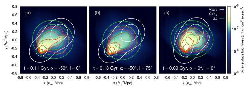
Figure 1: X-ray surface brightness, mass surface density, and SZ effect distributions for a merging cluster with the fiducial model A configuration, simulated by using the SPH code. Panels (a) and (b) show the results at different viewing directions, i.e., $(\alpha,\,i)=(-50\arcdeg,\,0\arcdeg)$ and $(-50\arcdeg,\,75\arcdeg)$, at an evolution time of $t=0.11$ and $0.13{\rm\,Gyr}$ after passing the pericenter, respectively. By these settings, the projected distance between the two progenitor clusters is roughly the same ($\sim 700\,h_{70}^{-1}{\rm\,kpc}$). Panel (c) shows the simulation results obtained from fiducial model A at the viewing direction of $(\alpha,\,i)=(0\arcdeg,\,0\arcdeg)$ at an evolution time of $t=0.09{\rm\,Gyr}$. The overlaid log-spaced contours represent the projected mass surface density (white; the ratio between two successive contour levels is 1.8), the X-ray surface brightness (red, the ratio between two successive contour levels is 1.8) and the SZ effect (green; the ratio between successive contour levels is 1.3). Panel (b) shows the merging configuration in the case A mergers that best matches to the observations (see Section 3.1).

Figure 2 shows the simulation results of several case A mergers, each with only one parameter, such as the initial relative velocity (panel (a)), the impact parameter (panel (b)), the core radius of the secondary cluster (panel (c)), or the mass ratio (panel (d)), different from those of fiducial model A. The snapshot time of each simulation shown in the figure is chosen to keep the projected separation of the two clusters to be consistent with the observation, as done above. This figure shows that the results obtained from those different parameters do not match the observations better than the result from fiducial model A. As seen from Figure 2(a) and Figure 1(b), the lower initial relative velocity results in a longer time required for the interaction of the gas halos of the two progenitor clusters and a longer time for the shocks to propagate farther away. Therefore, the shocks (i.e., wing-like structure) driven by the collision appear more significant in the X-ray map for the case of a merger with a lower initial relative velocity than that with a higher velocity. The shape of the X-ray emission in the central region thus tends to be more like a triangle (or a bullet) in the case with a lower initial relative velocity than that with a higher velocity. By comparing Figure 2(b) with Figure 1(b), we note that more distinct shocks can be formed through the merger with a smaller impact parameter than that with a larger impact parameter, as the collision with a smaller impact parameter is more violent. By comparing Figure 2(c) with Figure 1(b), we find that choosing a smaller core radius for the secondary cluster may lead to an increase of the X-ray emission in the center of the cluster; however, only one tail structure tracing the secondary cluster is formed, which is inconsistent with the observation. As seen from Figure 2(d) and Figure 1(b), the merger with a smaller secondary progenitor cluster (i.e., a large mass ratio $\xi$) is less violent and may not be able to destroy the gas core of the primary cluster; and in this case two peaks in the X-ray map may emerge, which is also in contradiction with the X-ray observation of ACT-CL J0102–4915.

Figure 2: Similar to those in Figure 1, but for the simulated merging clusters with initial configurations slightly different from that of fiducial model A. Panels (a), (b), (c), (d) show the results for the cases with only the relative velocity $V$ ($=1500{\rm\,km\,s^{-1}}$), the impact parameter $P$ ($=50\,h_{70}^{-1}{\rm\,kpc}$), the core radius of the secondary cluster $r_{\rm c}$ ($=r_{\rm s}/6$), or the mass ratio $\xi$ ($=4$) different from that for fiducial model A, respectively. The viewing direction is set to be the same, $(\alpha,\,i)=(-50\arcdeg,\,75\arcdeg)$ for all the four cases shown here. The snapshots shown in panels (a), (b), (c), (d) are at a time $t=0.17$, $0.16$, $0.14$, and $0.14{\rm\,Gyr}$, respectively, in order to keep the projected distance between the two clusters. See Section 3.1.

3.2 Case B Mergers

Case B mergers are offset collisions of two massive clusters with impact parameter $\gtrsim 500\,h_{70}^{-1}{\rm\,kpc}$, their collision strengths are less violent than those of the case A mergers. For case B mergers, the gas cores of the primary clusters are not always destroyed after the first pericentric passages; therefore, the merging systems may have two peaks in their X-ray maps. A single peak in the simulated X-ray map as that for ACT-CL J0102–4915 may be also produced if the gas fraction of the primary cluster is substantially lower than that of the secondary cluster, e.g., $f_{\rm b1}=0.05$, $f_{\rm b2}=0.10$; and the single peak is close to the center of the secondary cluster. By exploring the parameter space, we find that a merger with $(M_{1},\,\xi,\,f_{\rm b1},\,f_{\rm b2},\,V,\,P)=(2.5\times 10^{15}\,h_{70}^{-1}{\,M_{\odot}},\,3.6,\,0.05,\,0.10,\,2500{\rm\,km\,s^{-1}},\,800\,h_{70}^{-1}{\rm\,kpc})$ can match most of the observational features of ACT-CL J0102–4915, and the merger model defined by this parameter set is denoted as fiducial model B in the following text.

Figure 3 shows some snapshots of a merging system resulting from fiducial model B, viewing at $(t,\,\alpha,\,i)=(0.11{\rm\,Gyr},\,-90\arcdeg,\,0\arcdeg)$ (panel a), $(0.14{\rm\,Gyr},\,-90\arcdeg,\,30\arcdeg)$ (panel b), and $(0.19{\rm\,Gyr},\,-90\arcdeg,\,60\arcdeg)$ (panel c), respectively. As seen from Figure 3, a “wake” clearly exists trailing after the secondary cluster in the simulated X-ray image, which is quite similar to the observational one of ACT-CL J0102–4915 (Menanteau et al., 2012). The “wake” structure is more evident if viewing the merging system at the direction with $i\sim 0\arcdeg-30\arcdeg$, which suggests that the merger event of ACT-CL J0102–4915 should take place in a plane close to the sky plane, consistent with the argument presented in Menanteau et al. (2012). The simulation results presented in Figure 3(b) appear to match the observations the best. For example, the projected distance between the centers of the two clusters in this simulation is about $780\,h_{70}^{-1}{\rm\,kpc}$, roughly consistent with the observations; the morphologies of the X-ray emission, the mass surface density, and the SZ effect also match the observations well (see Fig. 1 in Menanteau et al. 2012).

We further investigate the gas distribution in the simulated merging cluster resulting from fiducial model B, in order to understand the origin of the wake shown in Figure 3. Figure 4 shows the projected distribution of gas particles for the snapshot shown in Figure 3(b), where the purple and the blue points represent some gas particles randomly selected from those in the primary and the secondary clusters, respectively. As seen from Figure 4, the gas core of the primary cluster is significantly displaced from the center of its gravitational potential well (mainly determined by the distribution of DM particles) because of the dissipative nature of the gas collision; the distribution of gas particles originally in the secondary cluster becomes elongated due to the compression by the ram pressure from the primary cluster. The gas particles from the primary and the secondary clusters have not effectively mixed yet. Because of the large impact parameter of the case B mergers, the resulting two wings in the X-ray morphology are not as obvious as those resulting from the case A mergers. Gas particles from the secondary and the primary clusters dominate the top and the bottom parts of the wake, respectively, while the gas density is low in the middle part of the wake. In this case, the wake emerges mainly as a result of the specific overlapping positions of the disturbed gas halos, and it is unlikely to be caused by the merger-driven turbulence argued in Menanteau et al. (2012, see section 4.3 therein).

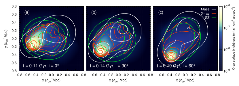
Figure 3: Similar to those in Figure 1, but for a merging cluster with the fiducial model B configuration. The viewing direction is set to $\alpha=-90\arcdeg$ and $i=0\arcdeg$, $30\arcdeg$, and $60\arcdeg$, at the merging time of $t=0.11$ (panel (a)), $0.14$ (panel (b)), and $0.19{\rm\,Gyr}$ (panel (c)), respectively. This figure shows that a wake (with two tails) trailing after the secondary cluster can be produced by a merger with the fiducial model B configuration. Panel (b) shows the merging configuration in the case B mergers that best matches the observations (see Section 3.2).

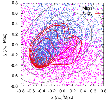
Figure 4: Projected distribution of gas particles of a merging cluster simulated by adopting the fiducial model B configuration and viewing at the merging time $t=0.14{\rm\,Gyr}$ and at a direction of ($\alpha=-90\arcdeg,\,i=30\arcdeg$). The purple and blue points represent the gas particles randomly selected from the primary and the secondary clusters, respectively. Red contours are the levels of the X-ray surface brightness (log-spaced, $5.6\times 10^{-7}$ to $10^{-8}\,{\rm cnt\,s^{-1}\,cm^{-2}\,arcsec^{-2}}$ from the inner ones to the outer ones), and the grey ones are the mass surface density (log-spaced, $0.56$ to $0.10\,{\rm g\,cm^{-2}}$ from the inner ones to the outer ones). This figure shows that the top and the bottom parts of the wake are dominated by the gas particles from the secondary and the primary clusters, respectively. See Section 3.2.

Figure 5 shows the simulation results on the X-ray surface brightness, the mass surface density, and the SZ effect distributions obtained from some of the case B mergers simulated in this study, each with one or two parameters different from those of fiducial model B. The snapshot time of each simulation shown in the figure is chosen to keep the projected separation of the two clusters to be consistent with the observation, as done above. As seen from the figure, the results obtained from those different parameters do not match the observations better than the result from fiducial model B. The detailed effects of those different parameters on the resulting maps are listed as follows.

• Panels (a) and (b) show a merger with only initial $V$ ($=1500{\rm\,km\,s^{-1}}$ and $3500{\rm\,km\,s^{-1}}$, respectively) different from that of fiducial model B. In the low-velocity case, the resulting maps appear to be similar to those of fiducial model B (Fig. 3b). However, in the high-velocity case, the bottom part of the wake becomes much stronger because of the shorter interaction time between the two clusters. If an even lower relative velocity is chosen, e.g., $V=500{\rm\,km\,s^{-1}}$, there is only one tail trailing after the secondary cluster in the resulting X-ray morphology. Therefore, $V\sim 1500-2500{\rm\,km\,s^{-1}}$ is required in order to reproduce ACT-CL J0102–4915 in the case B merger scenario, which is relatively lower compared with that for fiducial model A.

• Panel (c) shows a merger with only $f_{\rm b1}$ ($=0.10$) different from that of fiducial model B. In this case, the gas cores of the two progenitor clusters preserve themselves before the secondary pericentric passage, and thus two peaks emerge in the resulting X-ray map, which is apparently inconsistent with the X-ray observation of ACT-CL J0102–4915. In order to produce a single X-ray peak by the case B merger scenario, the gas fraction of the primary cluster must be lower than that of the secondary, and the gas fraction of the secondary cluster should also not be too large to form an unrealistic bright gas core in the center (e.g., $<0.13$).

• Panel (d) shows a merger with only the mass ratio $\xi$ ($=2$) different from that of fiducial model B. Apparently, the wake generated in this case is more asymmetric compared to that resulting from fiducial model B ($\xi=3.6$). We also find that the merger with a mass ratio of $5$, even smaller than that of fiducial model B, however, results in a more asymmetric X-ray morphology as well. According to those simulations, we conclude that a mass ratio of $\xi\sim 3.6$ is preferred in order to re-produce the wake shown in the X-ray map of ACT-CL J0102–4915.

• Panel (e) shows a merger with only the core radius of the secondary cluster $r_{\rm c}(=r_{\rm s}/6)$ different from that of fiducial model B. In this case, the resulting core of the X-ray emission is brighter and the gradient of the X-ray emission is larger, compared with those resulting from fiducial model B.

• Panel (f) shows a merger with only the primary cluster mass ($M_{1}=1.6\times 10^{15}\,h_{70}^{-1}{\,M_{\odot}}$) and the impact parameter ($P=600\,h_{70}^{-1}{\rm\,kpc}$) different from those of fiducial model B. Compared to fiducial model B, a smaller $P$ is adopted here because of the smaller size of the adopted system. The shapes of the X-ray surface brightness distribution and the SZ effect shown in panel (f) are similar to those in Figure 3(b); however, the total X-ray luminosity resulting from this merging system is substantially smaller than that from fiducial model B. In the case B scenario, a more massive merging system (e.g., $M_{1}=2.5\times 10^{15}\,h_{70}^{-1}{\,M_{\odot}}$) is required in order to generate the total X-ray luminosity of ACT-CL J0102–4915. Further discussion on the X-ray luminosity is detailed in Section 3.3.3.

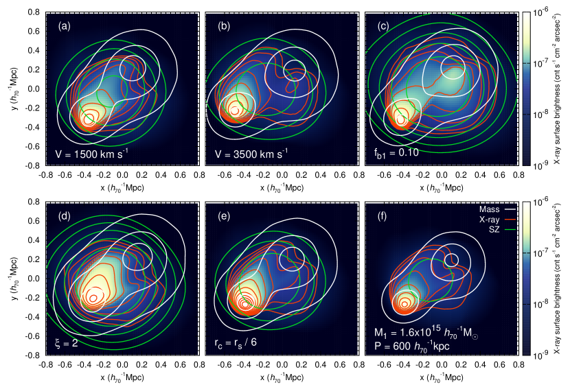
Figure 5: Similar to that for Figure 2, but for simulated merging clusters with initial configurations slightly different from that of fiducial model B. Panels (a)–(f) show the results for the cases with only the following parameters as labeled in each panel different from those of fiducial model B: initial relative velocity $V$ ($=1500{\rm\,km\,s^{-1}}$ and $3500{\rm\,km\,s^{-1}}$), gas fraction of the primary cluster $f_{\rm b1}$ ($=0.10$), mass ratio $\xi$ ($=2$), core radius of the secondary cluster $r_{\rm c}$ ($=r_{\rm s}/6$), and mass $M_{1}$ ($=1.6\times 10^{15}\,h_{70}^{-1}{\,M_{\odot}}$) and impact parameter $P$ ($=600\,h_{70}^{-1}{\rm\,kpc}$). The viewing direction is fixed at $(\alpha,\,i)=(90\arcdeg,\,-30\arcdeg)$. The snapshots shown in panels (a)–(f) are at a time $t=0.15$, $0.11$, $0.14$, $0.11$, $0.12$, and $0.14{\rm\,Gyr}$, respectively, in order to keep the projected distance between the two clusters. Apparently, fiducial model B gives a better match to the observations of ACT-CL J0102–4915, compared with those cases shown in this figure. See Section 3.2.

3.3 FLASH Simulation Results and Comparison to Observations

By surveying the parameter space of mergers of massive clusters, we find that fiducial model B or A may be the solution to the unique observational features of ACT-CL J0102–4915. The initial conditions are summarized in Table 2. For a detailed comparison, we re-run the simulations for fiducial models A and B by using the FLASH code, respectively, because the FLASH code handles shocks better than the GADGET-2 code. Figure 6 shows the results obtained from the FLASH simulations of fiducial models A (left panel) and B (right panel), respectively. We find that the main merging structures obtained from the FLASH simulations are well consistent with those obtained from the GADGET-2 simulations (see Figs. 1b and 3b for comparison; for example, the difference between the amplitudes of the X-ray peaks obtained from the two codes is not more than $5\%$.), except that the shock structures resulting from the FLASH simulations are sharper. This consistence supports the robustness of our method, i.e., first surveying the parameter space of cluster mergers and singling out the parameter set(s) that can lead to a close match to the observations of ACT-CL J0102–4915 through efficient GADGET-2 simulations, and then mining out the details of the singled-out mergers by doing the FLASH simulations. Below we present the comparison between the FLASH simulation results and the observations of ACT-CL J0102–4915 in several different aspects, i.e., the X-ray surface brightness distribution, the positions of the centroids of the X-ray emission and the SZ effect, the total X-ray luminosity and the temperature distributions of electrons in the merging cluster, the Mach number crossing the shock discontinuity, and the relative radial velocity between the NW and the SW components of the cluster, respectively. The main results are summarized in Table 2.

Table 2: Summary of the initial conditions and the cluster properties in the models and observations

Initial conditions
	Model A	Model B	Extended Model B	MB model
$M_{1}\ (10^{15}{\,M_{\odot}})$	$1.3$	$2.5$	$2.5$	$1.4$
$\xi$	$2.0$	$3.6$	$3.6$	$1.9$
$(f_{\rm b1},\,f_{\rm b2})$	($0.10,\,0.10$)	($0.05,\,0.10)$	($0.11,\,0.12)$	$(0.14,\,0.14)$
$V\ ({\rm\,km\,s^{-1}})$	$3000$	$2500$	$2500$	$2250$
$P\ (\,h_{70}^{-1}{\rm\,kpc})$	$300$	$800$	$800$	$300$
Gas density	Burkert	Burkert	Power law	non-isothermal/Burkert
profile
Measurements in the models and observations
	Model A	Model B	Extended model B	MB model	Observation
$t\ ({\rm\,Gyr})$	$0.13$	$0.14$	$0.17$	$0.42$	–
$(\alpha,\,i)$	($-50\arcdeg,\,75\arcdeg$)	($-90\arcdeg,\,30\arcdeg$)	($-90\arcdeg,\,40\arcdeg$)	($-90\arcdeg,\,55\arcdeg$)	–
$d_{\rm m}\ (\,h_{70}^{-1}{\rm\,kpc})$	$740$	$780$	$890$	$930$	$\sim 700$
$d_{\rm SZ-X}\ (\,h_{70}^{-1}{\rm\,kpc})$	$400$	$440$	$570$	$790$	$\sim 600$
Wake-like	No	Yes	Yes	Yes	Yes
structure		(the best match)
$\delta T_{0}\ ({\rm\mu K})$	$-1430$	$-1130$	$-1850$	$-1030$	$-1046\pm 116$
$L_{\rm X}$	$2.48\pm 0.03$	$2.05\pm 0.03$	$2.08\pm 0.03$	$1.77\pm 0.13$	$2.19\pm 0.11$
$(10^{45}{\,h_{70}^{-2}}{\rm\,erg}{\rm\,s^{-1}})$
$T_{\rm X}\ ({\rm\,keV})$	$15.8\pm 1.2$	$15.0\pm 1.3$	$18.0\pm 1.8$	$9.9\pm 0.6$	$14.5\pm 1.0$
$\mathcal{M}$ (SE, NW)	$(2.9,\,2.4)$	$(2.7,\,2.5)$	$(2.4,\,1.5)$	$(4.6,\,-)$	$(-,\,2.5^{+0.7}_{-0.3})$
$V_{\rm r}\ ({\rm\,km\,s^{-1}})$	$960$	$1820$	$2060$	$640$	$-$
	$(560)$	$(910)$	$(1200)$	$(590)$	$(586\pm 96$ / $731\pm 66)$
X-ray extension	No	No	Yes	Yes	Yes

Note. —  Lists of the initial conditions for different models (i.e., fiducial model A, fiducial model B, extended model B, and MB model) and comparison of the measurements between the models and the observations (Menanteau et al., 2012; Jee et al., 2014; Lindner et al., 2014).

3.3.1 Morphology of the X-Ray Surface Brightness and SZ Temperature Decrement

As seen from the left panel of Figure 6, we find the following points for fiducial model A. (1) The simulated morphology of the X-ray emission has a cometary appearance, which is consistent with the Chandra X-ray image of ACT-CL J0102–4915 (Menanteau et al., 2012). However, our simulation cannot produce a wake-like feature trailing after the secondary cluster as seen in ACT-CL J0102–4915. (2) The core of the simulated X-ray emission is not as bright as the observational one, because the gas in the core of the secondary cluster is partly stripped off due to the nearly head-on collision, which leads to a fainter X-ray core. Setting a smaller core radius $r_{\rm c}$ for the secondary cluster (Eq. 2), may reduce this inconsistency but result in some other inconsistency (see Figs. 2c and 5e).

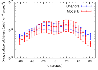
Figure 8: X-ray surface brightness distribution across the wake of ACT-CL J0102–4915 from the red boxes in Figure 7. The twin-tailed structure resulting from fiducial model B (red) can well match that of the Chandra observation (blue). See Section 3.3.1.

As seen from the right panel of Figure 6, we find the following points for fiducial model B. (1) The gas core of the smaller cluster survives after the first pericentric passage. The X-ray emission core is slightly brighter than the observational one. (2) A remarkable wake-like feature, similar to the observation, is reproduced. Figure 8 shows the comparison between the X-ray surface brightness across the wake resulting from fiducial model B and that from the Chandra observation. As seen from this figure, the simulation results can well match the twin-tailed structure found by the Chandra observation. (3) The morphology of the X-ray emission in the inner region (see Fig. 7, the inner regions 1, 2, and 3) of the merging system is roughly the same as the observations.

For both fiducial models A and B, the resulting X-ray surface brightness distribution rapidly decreases to an extremely low level at the outer region (regions 4 and 5 marked in Figs. 7b1 and 7c1) of the merging system. However, the X-ray emission of ACT-CL J0102–4915 extends to a relatively large scale ($\sim 1\,h_{70}^{-1}{\rm\,Mpc}$) and the decrease of the surface brightness is not as steep as the simulation ones at the outer region (see a careful comparison shown in Fig. 7). We note here that (1) considering the contamination from the CXB cannot solve this discrepancy; (2) increasing the total mass of the merging system does not lead to a better match to the X-ray morphology, especially for the extended X-ray emission in the outer region; and (3) choosing a snapshot at a later merging time does not lead to a significant improvement in matching the X-ray morphology (cf. the MB model), either. In our simulations, a given gas fraction normalized at the radius $r_{200}$ is adopted for the gas density distribution, which might not represent the real distribution well (see Fig. 11). We find that setting a cumulative gas fraction as a function of the radius for the primary cluster ($f_{\rm b1}\sim 0.05$ at $0.1r_{\rm 200}$ and $f_{\rm b1}\sim 0.11$ at $r_{\rm 200}$, motivated by the cosmological simulations and the X-ray observations; Battaglia et al. 2013; Mantz et al. 2014) could either solve the above discrepancy or provide a natural explanation to the low gas fraction of the primary cluster required in fiducial model B (denoted as extended model B). More discussions are in Section 3.4.

Because of the limited angular resolution of the SZ observation (i.e., $1.4^{\prime}$ of ACT at 148 GHz), we focus on the central temperature decrement of the SZ effect but not the morphology. The strength of the SZ signal at the center for fiducial models A and B is $-1430$ and $-1130\,{\rm\mu K}$, respectively. The result from model B is in agreement with the measured temperature decrement of ACT-CL J0102–4915, i.e., $-1046\pm 116\,{\rm\mu K}$, in Marriage et al. (2011). However, the result from fiducial model A is about $30\%$ larger. It is worth noting that the non-thermal pressure, which is not considered in this study, may have a non-negligible effect on modeling the SZ emission (Battaglia et al., 2012), and thus the central temperature decrement of the SZ effect obtained in the models may be overestimated by dozens of percent (Trac et al., 2011; Bode et al., 2012).

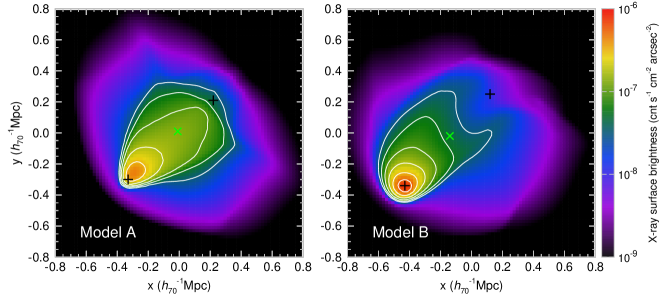
Figure 6: X-ray surface brightness distributions obtained from the FLASH simulations. Left and right panels show the results for fiducial models A and B, respectively. In each panel, the symbols ‘+’ (black) and ‘$\times$’ (green) symbols mark the positions of the mass centers of the two clusters and the centroid of the SZ map, respectively. The white log-spaced contours represent the levels of X-ray brightness of $3.2\times 10^{-8}$, $5.6\times 10^{-8}$, $10^{-7}$, $1.8\times 10^{-7}$, $3.2\times 10^{-7}$, and $5.6\times 10^{-7}$ from outside to inside, respectively. The morphological features of fiducial Model A and B are summarized in Table 2. See also Section 3.3.1.

3.3.2 Peak Positions of the X-Ray and SZ Emissions

Positions of the peaks of the X-ray emission and the SZ effect of merging clusters contain abundant information about the merging process. Different dependences of the X-ray and the SZ signals on the gas density and temperature distributions may induce a significant SZ-X-ray offset in a massive merging system after the first pericentric passage, when the X-ray peak locates near the center of the secondary cluster (i.e., the “jump effect”, see the demonstration in Zhang et al. 2014) and the SZ peak locates close to the center of the primary cluster. ACT-CL J0102–4915 is a typical example, of which the SZ-X-ray offset is about $600\,h_{70}^{-1}{\rm\,kpc}$ (Menanteau et al., 2012).

The SZ-X-ray offsets obtained from fiducial models A and B are both close to $400\,h_{70}^{-1}{\rm\,kpc}$, somewhat smaller than that given by observations (i.e., $600\,h_{70}^{-1}{\rm\,kpc}$). The SZ centroids resulting from the models are separated from the centers of the primary clusters by $280\,h_{70}^{-1}{\rm\,kpc}$, which are somewhat larger than that of ACT-CL J0102–4915 reported in Jee et al. (2014, $\sim 150\,h_{70}^{-1}{\rm\,kpc}$). Considering the low angular resolution of the SZ observation, the uncertainty in the SZ centroid estimate is $\sigma_{\rm peak}\sim 1.4^{\prime}/{\rm SNR}\sim 70\,h_{70}^{-1}{\rm\,kpc}$. The differences between the model results and the observations on the SZ-X-ray offset or the separation between the SZ centroid and the mass center of the primary cluster are about the same as the uncertainty, which suggests that our model results are roughly consistent ($\sim 2\sigma_{\rm peak}$) with the observations on these aspects.

For ACT-CL J0102–4915, Jee et al. (2014) found that the distance between the centroid of the X-ray emission and the center of the secondary cluster is $\sim 60\,h_{70}^{-1}{\rm\,kpc}$; and the X-ray centroid leads the mass surface density peak of ACT-CL J0102–4915 if the merging cluster is viewed soon after the first core passage. The spatial offsets between the X-ray centroid and the secondary cluster center of the simulated merging clusters are $\sim 50\,h_{70}^{-1}{\rm\,kpc}$ in fiducial model A and $\sim 5\,h_{70}^{-1}{\rm\,kpc}$ in the fiducial model B, respectively. However, it appears that the X-ray centroid resulting from model A or model B does not lead the mass surface density peak in the direction as shown in the observation. Furthermore, we do not find any case whose X-ray centroid leads the mass surface density peak by more than $50\,h_{70}^{-1}{\rm\,kpc}$ among the simulated merging clusters. We further examine the two scenarios suggested in Jee et al. (2014), i.e., (1) the merger is viewed before the first apocentric passage, and has a low initial merger speed; (2) the merger is viewed after the first apocentric passage, and has a high initial merger speed; and we find that neither of them can be a good solution because of the mismatch between the simulated X-ray morphology and the observational one.

If viewing SZ emissions with a substantially higher angular resolution (i.e., $\sigma_{\rm SZ}=10\,h_{70}^{-1}{\rm\,kpc}$), we may see two peaks in the SZ map in fiducial model B (also in extended model B; see Section 3.4). The primary one is near the center of the primary cluster, and the secondary one is close to the center of the secondary cluster. However, no secondary SZ peak exists in the high-resolution SZ image of fiducial model A. Therefore, the future SZ observations with the detailed substructures of ACT-CL J0102–4915 may provide more constraints on the merging scenarios.

3.3.3 X-Ray Luminosity and Temperature Distributions

We obtain the mock Chandra X-ray images of merging clusters ($0.5-2.0{\rm\,keV}$) by considering the exposure correction and the adaptive kernel smoothing. The left panels of Figure 7 show the Chandra observation (panel (a1)) and the mock X-ray images obtained from fiducial models A (panel (b1)) and B (panel (c1)) , respectively, for which the original X-ray images are shown in Figure 6. As seen from the figure, the substructures (e.g., shocks, wake) in the mock images appear less sharp than those in the original images (see Fig. 6) because of the adopted smoothing over a large scale to mimic the Chandra observations. Compared to the observations, both models result in a more concentrated X-ray-emitting gas distribution as discussed in Section 3.3.1. Panel (d1) presents the results of extended model B (see Section 3.4).

We extract the mock Chandra spectrum from the MARX simulated images for both models, where the extraction region is set to those areas between the innermost and the outermost contours shown in each of the left panels of Figure 7, similar to the analysis performed for the X-ray observation of ACT-CL J0102–4915 in Menanteau et al. (2012). We fit the spectra by using the phabs*mekal model, and obtain the mean temperature of the merging system resulting from fiducial model A or B as $T_{\rm X}=(15.8\pm 1.2){\rm\,keV}$ or $(15.0\pm 1.3){\rm\,keV}$. Both values are consistent with that estimated for ACT-CL J0102–4915 (i.e., $T_{\rm X}=(14.5\pm 1.0){\rm\,keV}$).

The total X-ray luminosities obtained from the mock images in the $0.5-2.0{\rm\,keV}$ band are $(2.48\pm 0.03)\times 10^{45}$ (panel (b1)) and $(2.05\pm 0.03)\times 10^{45}{\,h_{70}^{-2}}{\rm\,erg}{\rm\,s^{-1}}$ (panel (c1)), respectively, which are similar to the observation of ACT-CL J0102–4915 (i.e., $(2.19\pm 0.11)\times 10^{45}{\,h_{70}^{-2}}{\rm\,erg}{\rm\,s^{-1}}$; see Menanteau et al. 2012).

The total mass of the merging system is $2.0\times 10^{15}\,h_{70}^{-1}{\,M_{\odot}}$ in fiducial model A, consistent with the old estimate ($(2.16\pm 0.32)\times 10^{15}\,h_{70}^{-1}{\,M_{\odot}}$) for ACT-CL J0102–4915 by Menanteau et al. (2012), whereas it is $3.2\times 10^{15}\,h_{70}^{-1}{\,M_{\odot}}$ in fiducial model B, consistent with the new estimate ($(3.13\pm 0.56)\times 10^{15}\,h_{70}^{-1}{\,M_{\odot}}$) obtained by using the weak-lensing technique in Jee et al. (2014). Considering the large uncertainties in those mass estimates and the possible bias due to the adoption of the X-ray mass proxies for unrelaxed clusters (see Nagai et al., 2007; Vikhlinin et al., 2009), both fiducial models A and B can be taken as roughly consistent with the observation in terms of the cluster mass. To further distinguish the two different merging scenarios, an accurate mass estimation is required.

We further investigate the temperature obtained from the mock X-ray emission from each region marked in the left panels of Figure 7 for the two fiducial models. The resulting temperature distributions against the X-ray emitting regions are shown in the right panels of Figure 7 for the Chandra observation (panel (a2)), fiducial model A (panel (b2)), and fiducial model B (panel (c2)), respectively. As seen from the figure, the temperature distributions are roughly consistent with the observational one obtained for ACT-CL J0102–4915, although the temperature uncertainties are larger than the observational ones because of the limited photon numbers in the outer regions resulting from both models.

We also reproduce the MB model (Molnar & Broadhurst, 2015) for ACT-CL J0102–4915 ($V=2250{\rm\,km\,s^{-1}},\,P=300\,h_{70}^{-1}{\rm\,kpc}$) by using the FLASH code, in order to compare our model results with theirs in detail. The main results are summarized in Table 2. We find that the X-ray emission resulting from the MB model extends to larger scales compared with those from fiducial models A and B, mainly due to a later merging stage adopted in the MB model. The SZ decrement at the center resulting from the MB model ($-1030\,{\rm\mu K}$) is also consistent with observations. However, its mean temperature and total X-ray luminosity are $(9.9\pm 0.6){\rm\,keV}$ and $(1.77\pm 0.13)\times 10^{45}{\,h_{70}^{-2}}{\rm\,erg}{\rm\,s^{-1}}$, respectively, substantially lower than those from the observations and our models.

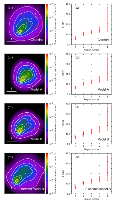
Figure 7: Left panels: image of the Chandra X-ray emission (panel (a1)), mock Chandra X-ray images resulting from fiducial model A (panel (b1)), fiducial model B (panel(c1)) and extended model B (panel (d1)). The contour levels are $0.29\times 10^{-8},\ 0.70\times 10^{-8},\ 1.8\times 10^{-8},\ 4.5\times 10^{-8}$, and $1.1\times 10^{-7}\,{\rm cnt\,s^{-1}\,cm^{-2}\,arcsec^{-2}}$ from outside to inside, respectively. The intersections of the X-ray surface brightness distribution across the wake region in the red boxes are shown in Figure 8 (see Section 3.3.1). Right panels: temperatures estimated from the spectra of X-ray emission from different extraction regions corresponding to the region number marked in the left panels (see Section 3.3.3). The red points are the result for the observation; the black points are those for the models, which are slightly shifted to the left to show a clear comparison with the observation. The maximums of the X-ray surface brightness in panels (b1) and (c1) are lower than those shown in Figure 6, because the exposure time of the mock Chandra X-ray images is limited and a larger smoothing scale is adopted in the images. The mock X-ray image and the temperature distribution of extended model B are similar to those of fiducial model B; but the X-ray emission in the outer region obtained from extended model B is stronger, which is comparable with that of the observation (see Section 3.4).

3.3.4 The Mach Number

Figure 10 shows the hydrodynamical quantities, i.e., the electron number density ($n_{\rm e}$), temperature ($T$), pressure ($P_{\rm g}$), and entropy (defined as $S\equiv k_{\rm B}Tn_{\rm e}^{-2/3}$), across the SE shock discontinuity (leading the secondary cluster) resulting from fiducial models A (left panels) and B (right panels), respectively. All those profiles are measured along the line across the centers of the two clusters (in the $z^{\prime}=0$ plane). The vertical dashed lines indicate the location of the bow shock. The Rankine–Hugoniot conditions are adopted to determine the Mach number $\mathcal{M}$ (see eqs. 89.6–89.8 in Landau & Lifshitz 1959). We estimate $\mathcal{M}$ from the jump in the temperature profile for its well-defined discontinuity, and find $\mathcal{M}=4.3$ and $3.8$ for fiducial models A and B, respectively. The expected jumps of other quantities from the Mach number are also shown as the horizontal dotted lines in Figure 10. The Mach number from the MB model that we reproduce by using the FLASH code is $\sim 6.0$.

In the models the NW and SE shocks (moving outward in front of the primary and secondary clusters, respectively) are coincident in positions with the observed radio relics of ACT-CL J0102–4915 (Lindner et al., 2014). To compare with the observations, we also estimate the Mach numbers of the SE and NW shocks from the spectroscopic-like temperature map (see eq. 6 in Mastropietro & Burkert (2008)). They are in general smaller than the actual values (measured in the $z^{\prime}=0$ plane) due to the projection effect (see Mastropietro & Burkert, 2008; Machado & Lima Neto, 2013). The inferred Mach numbers (SE, NW) for model A, model B, and the MB model are $(2.9,\,2.4)$, $(2.7,\,2.5)$, and $(4.6,\,-)$, respectively (no clear NW shock found in the MB model). The results of our fiducial models are both consistent with that reported in Lindner et al. (2014), where $\mathcal{M}=2.5^{+0.7}_{-0.3}$ is estimated from the spectral index of the NW radio relic of ACT-CL J0102–4915 (see the comparison between the Mach numbers derived from the X-ray and the radio observations in Akamatsu & Kawahara (2013)). A tight constraint on the Mach numbers derived from the temperature profile across the SE and NW shocks in the X-ray observation may provide additional information to distinguish or falsify fiducial models A and B proposed in this study and the models in Molnar & Broadhurst (2015).

3.3.5 The Relative Radial Velocity

Menanteau et al. (2012) estimate the observed relative radial velocity along the LOS ($586\pm 96{\rm\,km\,s^{-1}}$) between the two components (NW and SE) of ACT-CL J0102–4915 based on the galaxy redshift distribution, while the observed relative radial velocity between the NW component and the cluster BCG located in the SE component is $731\pm 66{\rm\,km\,s^{-1}}$. The relative radial velocities resulting from fiducial model A and fiducial model B are $960{\rm\,km\,s^{-1}}$ and $1820{\rm\,km\,s^{-1}}$ respectively, which are directly estimated from the peculiar velocities of the NW and the SE mass centers. However, it appears that our model results may not be in contradiction with the observations, because the values of the relative radial velocities are obtained from different methods and the observationally determined values may not reveal the real relative radial velocities of the mass centers.

The values of relative radial velocities obtained from different methods may differ from each other significantly (e.g., by a factor of 2). To illustrate this point, we model the velocity distributions for the DM particles in the NW and the SE cluster components of fiducial models A and B in Figure 9, where the DM particles separated from the NW or the SE mass centers within a projected distance of $400\,h_{70}^{-1}{\rm\,kpc}$ on the plane of the sky are referred to as the NW or the SE cluster component. The relative radial velocities measured from the best-fit Gaussian distributions for the NW and the SE velocity distributions (see dashed lines in the figure) are $560$ and $910{\rm\,km\,s^{-1}}$ for fiducial models A and B, respectively, which are significantly lower than the real ones, but generally consistent with the observational values. The reason for the low values obtained in Figure 9 is that the DM particles (or the galaxies in the observations) are grouped into two subsets by their projective distances to the NW and the SE mass centers, respectively; and the merging process has destroyed the boundaries of the original clusters, so that the SE (NW) subset contains the particles or galaxies initially belonging to the NW (SE) cluster (whose velocities, however, are still close to their original host). Figure 9 indicates that the measurement used in Menanteau et al. (2012) may underestimate the relative velocity between the two clusters significantly. Note that the degree of the underestimate depends on the overlapping fraction of the two clusters along the LOS. For example, if the two clusters are at a relatively later merging stage after the pericentric passage so that they have a larger separation and less overlapped, the underestimate may be significantly smaller than the factor of 2.

In addition to the above significant factor, the relative radial velocity estimations may be also affected by a few other factors. (a) The velocities inferred from different components (e.g., DM, galaxies) within a cluster are different (Dolag & Sunyaev, 2013). For ACT-CL J0102–4915, the observed relative radial velocity is estimated from the motions of galaxies, while the velocity resulting from the model is based on the motions of DM particles. This difference could introduce an error on the order of $100{\rm\,km\,s^{-1}}$. (b) The relative radial velocity resulting from a model is also sensitive to the choice of the projection angle $\alpha$ and $i$. If choosing $i=15\arcdeg$ rather than $30\arcdeg$ in fiducial model B (the X-ray morphology does not differ significantly), the relative radial velocity decreases by a factor of $\sim$2.

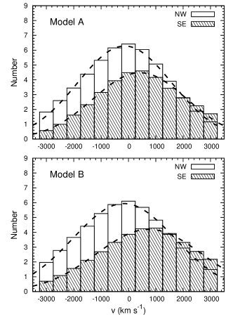
Figure 9: Radial velocity distributions along the LOS of the DM particles in the NW and the SE cluster components for fiducial model A (top panel) and fiducial model B (bottom panel). The distributions for the NW and the SE components are normalized to 51 and 36 in the total number to directly compare with the observations shown in fig. 9 in Menanteau et al. 2012. The dashed lines give the best-fit Gaussian distributions for the velocity distributions. The relative radial velocities measured from the best fits are $560$ and $910{\rm\,km\,s^{-1}}$ for fiducial model A and fiducial model B, respectively. The values are significantly smaller than the real relative velocity of the mass centers ($960$ and $1820{\rm\,km\,s^{-1}}$, respectively) but generally consistent with the observations, which illustrates that the observational estimates may be significantly biased and underestimate the relative radial velocity between the NW and SE cluster components. See Section 3.3.5.

Figure 10: Electron number density, gas temperature, pressure, and entropy profiles across the SE shock discontinuity resulting from fiducial model A (left panels) and fiducial model B (right panels). The vertical dashed lines mark the location of the bow shock. The center of the secondary cluster is at $d=0$. The Mach number ${\mathcal{M}}$ determined from the discontinuity in the temperature profile is $\mathcal{M}=4.3$ and $3.8$ for fiducial models A and B, respectively. The dotted horizontal lines give the expected jump of the quantities from the obtained Mach number. See Section 3.3.4.

3.4 Discussion on the Effects of the Gas Fraction Profile

According to the simulations, fiducial model B could reproduce most of the observational features of ACT-CL J0102–4915, but with two deficiencies: (1) less X-ray emission is produced in the outer region of the merging cluster compared with the observations (see Section 3.3.1); (2) the adopted gas fraction of the primary cluster ($0.05$) is substantially lower than the typical value of massive galaxy clusters ($\sim 0.13$). The simplified gas density distribution for the galaxy clusters in the simulation results in an approximately flat cumulative gas fraction profile while $r>0.2r_{\rm 200}$, which, however, does not well represent the situations in the observations and cosmological simulations (Battaglia et al., 2013; Mantz et al., 2014). We find that setting the cumulative gas fraction as a function of the radius following the constraints from the observations may solve the above discrepancies. We further perform simulations with different gas density profiles described below, denoted as the extended case B mergers, by using the GADGET-2 code. For the primary cluster, we assume that the cumulative gas fraction profile follows a power-law form,

$$f_{\rm b1}(<r)=A\left(\frac{r}{r_{\rm f}}\right)^{\gamma},$$ (7)

where $r_{\rm f}\equiv 0.1r_{\rm 200}$ is the scale radius. The gas density distribution can then be numerically determined from the enclosed DM mass distribution. For the secondary cluster, the gas density distribution still follows the Burkert profile (see Eq. 2) as that in fiducial model B, but with two differences, i.e., $f_{\rm b2}=0.12$ and $r_{\rm c}=r_{\rm s}/2$. We find that the simulation results with the relatively large gas core size of the secondary cluster ($\sim 100\,h_{70}^{-1}{\rm\,kpc}$) give a good match to ACT-CL J0102–4915. As an example, we show the different cumulative gas fraction profiles adopted in the extended case B mergers when $A$ is set to $0.045$ in Figure 11. In the central region ($\sim 0.05-0.3r_{\rm 200}$), the gas fractions in Equation (7) are close to $0.05$, similar to that of fiducial model B; at the radius $r_{200}$, the gas fractions are $0.07,\,0.11,\,0.18$ for those cases with $\gamma=0.2,\,0.4,\,0.6$, respectively, generally consistent with the observational constraints from the observations (Mantz et al., 2014). It is worth noting that the power-law form for the cumulative gas fraction profile is unrealistic for the outer region of the galaxy clusters when the gas fraction is much higher than the cosmological average value (e.g., $r>2r_{\rm 200}$ for the $\gamma=0.4$ case), which, however, has little effect on our results since the DM density distribution drops significantly outside $r_{\rm 200}$ in our models. The merger configuration of the extended case B mergers follows that of fiducial model B with the parameter set $(M_{1},\,\xi,\,V,\,P)=(2.5\times 10^{15}\,h_{70}^{-1}{\,M_{\odot}},\,3.6,\,2500{\rm\,km\,s^{-1}},\,800\,h_{70}^{-1}{\rm\,kpc})$.

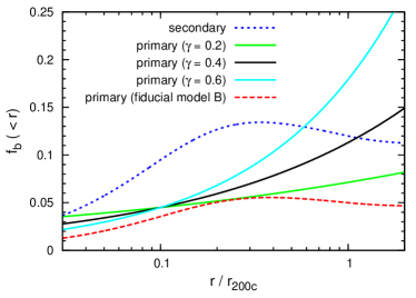
Figure 11: Cumulative gas fraction profiles for the primary and the secondary clusters. The green, black, and cyan solid lines represent the profiles of the primary clusters following Equation (7) with $A=0.045$ and $\gamma=0.2,\,0.4$, and 0.6, respectively. The blue dotted line represents the profile of the secondary cluster in the extended case B mergers. The red dashed line represents the profile of the primary cluster in fiducial model B. In the central region, the profiles shown by the solid lines are close to that of fiducial model B; but at the radius $r_{200}$, the gas fractions shown by the solid lines are all higher than $0.05$. See Section 3.4.

Figure 12 shows the simulation results for the different cumulative gas fraction profiles (i.e., $\gamma=0.2,\,0.4$ and 0.6), which correspond to the solid lines in Figure 11, respectively. As seen from Figure 12, the simulation results presented in panel (b) are quite similar to those of fiducial model B (see Fig. 3b), but the X-ray emission in the outer region of the merging cluster increases as the gas fraction at the virial radius becomes higher. Panel (a) shows a highly asymmetric twin-tailed structure in the X-ray image and a remarkable secondary X-ray peak close to the center of the primary cluster, which do not match the observations well. Unlike that in panel (b), the secondary X-ray peak in panel (a) is still clear in its mock Chandra X-ray image. Panel (c) also fails to reproduce the observations since no clear wake-like structure appears in the X-ray image. Furthermore, the different cumulative gas fraction profiles with $A=0.03$ and $0.06$ are also tested. We find that $A=0.045$ is preferred to match the X-ray luminosity of ACT-CL J0102–4915.

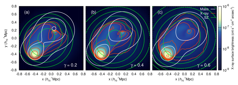
Figure 12: Similar to those in Figure 1, but for the simulated merging clusters in the extended case B mergers (where the cumulative gas fraction profile follows Equation (7)). Panels (a), (b), (c) show the results for the cases with $\gamma=0.2,\,0.4$, and 0.6, respectively, and $A$ is fixed to $0.045$. The viewing direction is set to be the same with $(\alpha,\,i)=(-90\arcdeg,\,40\arcdeg)$ for all the three cases. The merging time for the three snapshots is $t=0.17{\rm\,Gyr}$. The simulation results of panel (b) are similar to those of fiducial model B, but with stronger X-ray emission in the outer region of the merging cluster. See Section 3.4.

We further re-run a FLASH simulation for the extended case B merger with $A=0.045,\,\gamma=0.4$ (denoted as extended model B) and compare the model with the observations as done in Section 3.3. The main results are summarized in Table 2 (see also Figs. 7d1 and 7d2). We find the following points for extended model B. (1) The mock X-ray image and the temperature distribution are similar to that of fiducial model B (see Figs. 7c1 and 7c2). But the X-ray emission in the outer region obtained from extended model B is more significant, which is comparable with the observational one. (2) The total X-ray luminosity in the $0.5-2.0{\rm\,keV}$ band and the best-fitted X-ray temperature are $(2.08\pm 0.03)\times 10^{45}{\,h_{70}^{-2}}{\rm\,erg}{\rm\,s^{-1}}$ and $(18.0\pm 1.8){\rm\,keV}$, respectively. The Mach number across the SE shock (measured in the $z^{\prime}=0$ plane) is $3.1$, and the relative radial velocity between the two clusters is $2060{\rm\,km\,s^{-1}}$. The quantities above are all consistent with those of fiducial model B except that the temperature is about $20\%$ higher. (3) The central temperature decrement of the SZ effect of extended model B is, however, $-1850{\,\mu{\rm K}}$, much lower than the measurement of ACT-CL J0102–4915. The non-thermal pressure may play a non-negligible role in this situation; and ignoring the non-thermal pressure in our models may lead to the overestimation of the central temperature decrement by dozens of percent (see Battaglia et al. 2012; Lau et al. 2009).

4 Conclusion

In this work, we perform a series of simulations of mergers of two galaxy clusters in order to investigate the merging scenario and identify the initial conditions for ACT-CL J0102–4915. By surveying over the space of those parameters that define the merger configuration, including the mass of the primary cluster, mass ratio, gas fraction, initial relative velocity, and impact parameter, we discuss two types of the merger configuration that may be able to reproduce the observations of ACT-CL J0102–4915, respectively. The first type is a nearly head-on merger with impact parameter $\sim 300\,h_{70}^{-1}{\rm\,kpc}$ (fiducial model A) and the second one is a highly off-axis merger with $\sim 800\,h_{70}^{-1}{\rm\,kpc}$ (fiducial model B). The detailed comparison of our simulation result with the observations of ACT-CL J0102–4915 is summarized in Table 2.

Fiducial model A is for an energetic collision of two clusters. In this model, the central gas core of the primary cluster is completely destroyed after the first core-core collision. The morphology of the X-ray surface brightness, the X-ray luminosity, and the temperature distributions of ACT-CL J0102–4915 can be reproduced, but no wake-like substructure trailing the secondary cluster is produced by the model. According to the simulations, fiducial model A is the merging configuration that best matches the observations when the impact parameter is smaller than $500\,h_{70}^{-1}{\rm\,kpc}$.

Fiducial model B is for a less energetic collision, compared with fiducial model A, as its impact parameter is much larger. A remarkable wake-like feature is clearly seen trailing after the secondary cluster, which is similar to that of ACT-CL J0102–4915. The total X-ray luminosity of a merging cluster is positively correlated with the total mass of the system, which may provide a strong constraint to the model. The total mass in fiducial model B is $3.2\times 10^{15}\,h_{70}^{-1}{\,M_{\odot}}$, consistent with the constraint from the weak-lensing technique (Jee et al., 2014). Our simulation results support that the NW subcluster of ACT-CL J0102–4915 is more massive than the SE one, in agreement with the measurement by Jee et al. (2014) but not that by Zitrin et al. (2013). The mass ratio between the NW and SE components of the cluster is $3.6$ for fiducial model B, which is somewhat higher than the estimate in Jee et al. (2014).

Fiducial model B can reproduce most of the basic features of ACT-CL J0102–4915, but it produces less X-ray emission in the outer region of the merging cluster compared to the observations. The reason might be that the adopted gas density profile in the model may not well represent the reality. Adopting the cumulative gas fraction as a function of the radius ($\sim 0.05$ at $0.1r_{\rm 200}$ and $\sim 0.11$ at $r_{\rm 200}$) motivated by observations (Mantz et al., 2014) can solve this discrepancy; and it may also provide a natural explanation to the low gas fraction ($0.05$) of the primary cluster assumed in fiducial model B. Compared with the models proposed in Molnar & Broadhurst (2015), fiducial model B presented in this paper appears to provide a better match to the X-ray morphology and the best-fit X-ray luminosity and temperature.

In this paper, the initial relative velocity of the two progenitor clusters of ACT-CL J0102–4915 is high, as suggested by fiducial model B ($\sim 2500{\rm\,km\,s^{-1}}$). The requirement of a high initial relative velocity for ACT-CL J0102–4915 may enhance the tension between the rarity of the high velocity mergers of clusters in cosmological simulations and the existence of the Bullet Cluster (e.g., Lee & Komatsu, 2010; Thompson & Nagamine, 2012, but Thompson et al. 2015), especially when considering the uncommon high mass (see more discussions in Jee et al. (2014)) and the small mass ratio of ACT-CL J0102–4915. According to fiducial model B, the highly off-axis merger configuration of ACT-CL J0102–4915 is different from that of the Bullet Cluster. Nevertheless, as ACT-CL J0102–4915 is extremely massive and rare at $z\sim 0.87$, the requirement of an extremely high initial relative velocity may present an even more significant challenge to our understanding of the structure formation compared to that by the Bullet cluster.

We thank David Spergel for bringing the galaxy cluster “El Gordo” to our attention. This research was supported in part by the National Natural Science Foundation of China under nos. 11273004, 11373031, and the Strategic Priority Research Program “The Emergence of Cosmological Structures” of the Chinese Academy of Sciences, Grant No. XDB09000000. The software used in this work was developed in part by the DOE NASA ASC- and NSF supported Flash Center for Computational Science at the University of Chicago. This research has made use of data obtained from the Chandra Data Archive and the software provided by the Chandra X-ray Center (CXC) in the application package CIAO.

References

- Agertz et al. (2007) Agertz, O., Moore, B., Stadel, J., et al. 2007, MNRAS, 380, 963
- Akamatsu & Kawahara (2013) Akamatsu, H., & Kawahara, H. 2013, PASJ, 65, 16
- Anders & Grevesse (1989) Anders, E., & Grevesse, N. 1989, Geochim. Cosmochim. Acta, 53, 197
- Battaglia et al. (2012) Battaglia, N., Bond, J. R., Pfrommer, C., & Sievers, J. L. 2012, ApJ, 758, 74
- Battaglia et al. (2013) Battaglia, N., Bond, J. R., Pfrommer, C., & Sievers, J. L. 2013, ApJ, 777, 123
- Binney & Tremaine (2008) Binney, J., & Tremaine, S. 2008, Galactic Dynamics: Second Edition (Princeton University Press)
- Bode et al. (2012) Bode, P., Ostriker, J. P., Cen, R., & Trac, H. 2012, arXiv:1204.1762
- Bouillot et al. (2014) Bouillot, V. R., Alimi, J.-M., Corasaniti, P.-S., & Rasera, Y. 2014, arXiv:1405.6679
- Burkert (1995) Burkert, A. 1995, ApJ, 447, L25
- Clowe et al. (2006) Clowe, D., Bradač, M., Gonzalez, A. H., et al. 2006, ApJ, 648, L109
- Clowe et al. (2004) Clowe, D., Gonzalez, A., & Markevitch, M. 2004, ApJ, 604, 596
- Colella & Woodward (1984) Colella, P., & Woodward, P. R. 1984, Journal of Computational Physics, 54, 174
- Dolag & Sunyaev (2013) Dolag, K., & Sunyaev, R. 2013, MNRAS, 432, 1600
- Donnert (2014) Donnert, J. M. F. 2014, MNRAS, 438, 1971
- Duffy et al. (2008) Duffy, A. R., Schaye, J., Kay, S. T., & Dalla Vecchia, C. 2008, MNRAS, 390, L64
- Fryxell et al. (2000) Fryxell, B., Olson, K., Ricker, P., et al. 2000, ApJS, 131, 273
- Hickox & Markevitch (2006) Hickox, R. C., & Markevitch, M. 2006, ApJ, 645, 95
- Itoh et al. (1998) Itoh, N., Kohyama, Y., & Nozawa, S. 1998, ApJ, 502, 7
- Jee et al. (2014) Jee, M. J., Hughes, J. P., Menanteau, F., et al. 2014, ApJ, 785, 20
- Kazantzidis et al. (2004) Kazantzidis, S., Magorrian, J., & Moore, B. 2004, ApJ, 601, 37
- Kraljic & Sarkar (2015) Kraljic, D., & Sarkar, S. 2015, JCAP, 4, 050
- Kravtsov & Borgani (2012) Kravtsov, A. V., & Borgani, S. 2012, ARA&A, 50, 353
- Lage & Farrar (2015) Lage, C., & Farrar, G. 2015, JCAP, 2, 38
- Landau & Lifshitz (1959) Landau, L. D., & Lifshitz, E. M. 1959, Course of theoretical physics, Oxford: Pergamon Press, 1959,
- Lau et al. (2009) Lau, E. T., Kravtsov, A. V., & Nagai, D. 2009, ApJ, 705, 1129
- Lee & Komatsu (2010) Lee, J., & Komatsu, E. 2010, ApJ, 718, 60
- Lindner et al. (2014) Lindner, R. R., Baker, A. J., Hughes, J. P., et al. 2014, ApJ, 786, 49
- Machado & Lima Neto (2013) Machado, R. E. G., & Lima Neto, G. B. 2013, MNRAS, 430, 3249
- Mantz et al. (2014) Mantz, A. B., Allen, S. W., Morris, R. G., et al. 2014, MNRAS, 440, 2077
- Markevitch et al. (2002) Markevitch, M., Gonzalez, A. H., David, L., et al. 2002, ApJ, 567, L27
- Marriage et al. (2011) Marriage, T. A., Acquaviva, V., Ade, P. A. R., et al. 2011, ApJ, 737, 61
- Mastropietro & Burkert (2008) Mastropietro, C., & Burkert, A. 2008, MNRAS, 389, 967
- Menanteau et al. (2012) Menanteau, F., Hughes, J. P., Sifón, C., et al. 2012, ApJ, 748, 7
- Milosavljević et al. (2007) Milosavljević, M., Koda, J., Nagai, D., Nakar, E., & Shapiro, P. R. 2007, ApJ, 661, L131
- Mitchell et al. (2009) Mitchell, N. L., McCarthy, I. G., Bower, R. G., Theuns, T., & Crain, R. A. 2009, MNRAS, 395, 180
- Molnar et al. (2012) Molnar, S. M., Hearn, N. C., & Stadel, J. G. 2012, ApJ, 748, 45
- Molnar & Broadhurst (2015) Molnar, S. M., & Broadhurst, T. 2015, ApJ, 800, 37
- Nagai et al. (2007) Nagai, D., Vikhlinin, A., & Kravtsov, A. V. 2007, ApJ, 655, 98
- Navarro et al. (1997) Navarro, J. F., Frenk, C. S., & White, S. D. M. 1997, ApJ, 490, 493
- Planck Collaboration et al. (2014) Planck Collaboration, Ade, P. A. R., Aghanim, N., et al. 2014, A&A, 571, AA29
- Ricker & Sarazin (2001) Ricker, P. M., & Sarazin, C. L. 2001, ApJ, 561, 621
- Ricker (2008) Ricker, P. M. 2008, ApJS, 176, 293
- Springel et al. (2001) Springel, V., Yoshida, N., & White, S. D. M. 2001, NewA, 6, 79
- Springel & Farrar (2007) Springel, V., & Farrar, G. R. 2007, MNRAS, 380, 911
- Thompson & Nagamine (2012) Thompson, R., & Nagamine, K. 2012, MNRAS, 419, 3560
- Thompson et al. (2015) Thompson, R., Davé, R., & Nagamine, K. 2015, MNRAS, 452, 3030
- Trac et al. (2011) Trac, H., Bode, P., & Ostriker, J. P. 2011, ApJ, 727, 94
- Vikhlinin et al. (2009) Vikhlinin, A., Burenin, R. A., Ebeling, H., et al. 2009, ApJ, 692, 1033
- Watson et al. (2014) Watson, W. A., Iliev, I. T., Diego, J. M., et al. 2014, MNRAS, 437, 3776
- Williamson et al. (2011) Williamson, R., Benson, B. A., High, F. W., et al. 2011, ApJ, 738, 139
- Zhang et al. (2014) Zhang, C., Yu, Q., & Lu, Y. 2014, ApJ, 796, 138
- Zitrin et al. (2013) Zitrin, A., Menanteau, F., Hughes, J. P., et al. 2013, ApJ, 770, L15
- ZuHone et al. (2009) ZuHone, J. A., Ricker, P. M., Lamb, D. Q., & Karen Yang, H.-Y. 2009, ApJ, 699, 1004