Autotuning OpenCL Workgroup Size for Stencil Patterns

Abstract

Selecting an appropriate workgroup size is critical for the performance of OpenCL kernels, and requires knowledge of the underlying hardware, the data being operated on, and the implementation of the kernel. This makes portable performance of OpenCL programs a challenging goal, since simple heuristics and statically chosen values fail to exploit the available performance. To address this, we propose the use of machine learning-enabled autotuning to automatically predict workgroup sizes for stencil patterns on CPUs and multi-GPUs.

We present three methodologies for predicting workgroup sizes. The first, using classifiers to select the optimal workgroup size. The second and third proposed methodologies employ the novel use of regressors for performing classification by predicting the runtime of kernels and the relative performance of different workgroup sizes, respectively. We evaluate the effectiveness of each technique in an empirical study of 429 combinations of architecture, kernel, and dataset, comparing an average of 629 different workgroup sizes for each. We find that autotuning provides a median $3.79\times$ speedup over the best possible fixed workgroup size, achieving 94% of the maximum performance.

1 Introduction

Stencil codes have a variety of computationally demanding uses from fluid dynamics to quantum mechanics. Efficient, tuned stencil implementations are highly sought after, with early work in 2003 by Bolz et al. demonstrating the capability of GPUs for massively parallel stencil operations [1]. Since then, the introduction of the OpenCL standard has introduced greater programmability of heterogeneous devices by providing a vendor-independent layer of abstraction for data parallel programming of CPUs, GPUs, DSPs, and other devices [2]. However, achieving portable performance of OpenCL programs is a hard task — OpenCL kernels are sensitive to properties of the underlying hardware, to the implementation, and even to the dataset that is operated upon. This forces developers to laboriously hand tune performance on a case-by-case basis, since simple heuristics fail to exploit the available performance.

In this paper, we demonstrate how machine learning-enabled autotuning can address this issue for one such optimisation parameter of OpenCL programs — that of workgroup size. The 2D optimisation space of OpenCL kernel workgroup sizes is complex and non-linear, making it resistant to analytical modelling. Successfully applying machine learning to such a space requires plentiful training data, the careful selection of features, and an appropriate classification approach. The approaches presented in this paper use features extracted from the architecture and kernel, and training data collected from synthetic benchmarks to predict workgroup sizes for unseen programs.

2 The SkelCL Stencil Pattern

Introduced in [3], SkelCL is an Algorithmic Skeleton library which provides OpenCL implementations of data parallel patterns for heterogeneous parallelism using CPUs and multi-GPUs. Figure 1 shows the components of the SkelCL stencil pattern, which applies a user-provided customising function to each element of a 2D matrix. The value of each element is updated based on its current value and the value of one or more neighbouring elements, called the border region. The border region describes a rectangular region about each cell, and is defined in terms of the number of cells in the border region to the north, east, south, and west of each cell. Where elements of a border region fall outside of the matrix bounds, values are substituted from either a predefined padding value, or the value of the nearest cell within the matrix, determined by the user.

When a SkelCL stencil pattern is executed, each of the matrix elements are mapped to OpenCL work-items; and this collection of work-items is divided into workgroups for execution on the target hardware. A work-item reads the value of its corresponding matrix element and the surrounding elements defined by the border region. Since the border regions of neighbouring elements overlap, each element in the matrix is read multiple times. Because of this, a tile of elements of the size of the workgroup and the perimeter border region is allocated as a contiguous block in local memory. This greatly reduces the latency of repeated memory accesses performed by the work-items. As a result, changing the workgroup size affects both the number of workgroups which can be active simultaneously, and the amount of local memory required for each workgroup. While the user defines the size, type, and border region of the matrix being operated upon, it is the responsibility of the SkelCL stencil implementation to select an appropriate workgroup size to use.

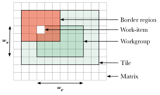
Figure 1: The components of a stencil: an input matrix is decomposed into workgroups, consisting of $w_{r}\times w_{c}$ elements. Each element is mapped to a work-item. Each work-item operates on its corresponding element and a surrounding border region (in this example, 1 element to the south, and 2 elements to the north, east, and west).

3 Autotuning Workgroup Size

Selecting the appropriate workgroup size for an OpenCL kernel depends on the properties of the kernel itself, underlying architecture, and dataset. For a given scenario (that is, a combination of kernel, architecture, and dataset), the goal of this work is to harness machine learning to predict a performant workgroup size to use, based on some prior knowledge of the performance of workgroup sizes for other scenarios. In this section, we describe the optimisation space and the steps required to apply machine learning. The autotuning algorithms are described in Section 4.

3.1 Constraints

The space of possible workgroup sizes $W$ is constrained by properties of both the architecture and kernel. Each OpenCL device imposes a maximum workgroup size which can be statically checked through the OpenCL Device API. This constraint reflects architectural limitations of how code is mapped to the underlying execution hardware. Typical values are powers of two, e.g. 1024, 4096, 8192. Additionally, the OpenCL runtime enforces a maximum workgroup size on a per-kernel basis. This value can be queried at runtime once a program has been compiled for a specific execution device. Factors which affect a kernel’s maximum workgroup size include the number of registers required, and the available number of SIMD execution units for each type of executable instruction.

While in theory, any workgroup size which satisfies the device and kernel workgroup size constraints should provide a valid program, in practice we find that some combinations of scenario and workgroup size cause a CL_OUT_OF_RESOURCES error to be thrown when the kernel is launched. We refer to these workgroup sizes as refused parameters. Note that in many OpenCL implementations, this error type acts as a generic placeholder and may not necessarily indicate that the underlying cause of the error was due to finite resources constraints. We define the space of legal workgroup sizes for a given scenario $s$ as those which satisfy the architectural and kernel constraints, and are not refused:

$$\footnotesize W_{legal}(s)=\left\{w|w\in W,w<W_{\max}(s)\right\}-W_{refused}(s)$$ (1)

Where $W_{\max}(s)$ can be determined at runtime prior to the kernels execution, but the set $W_{refused}(s)$ can only be discovered emergently. The set of safe parameters are those which are legal for all scenarios:

$$W_{safe}=\cap\left\{W_{legal}(s)|s\in S\right\}$$ (2)

3.2 Stencil and Architectural Features

Since properties of the architecture, program, and dataset all contribute to the performance of a workgroup size for a particular scenario, the success of a machine learning system depends on the ability to translate these properties into meaningful explanatory variables — features. For each scenario, 102 features are extracted describing the architecture, kernel, and dataset.

Architecture features are extracted using the OpenCL Device API to query properties such as the size of local memory, maximum work group size, and number of compute units. Kernel features are extracted from the source code stencil kernels by compiling first to LLVM IR bitcode, and using statistics passes to obtain static instruction counts for each type of instruction present in the kernel, as well as the total number of instructions. These instruction counts are divided by the total number of instructions to produce instruction densities. Dataset features include the input and output data types, and the 2D matrix dimensions.

3.3 Training Data

Training data is collected by measuring the runtimes of stencil programs using different workgroup sizes. These stencil programs are generated synthetically using a statistical template substitution engine, which allows a larger exploration of the program space than is possible using solely hand-written benchmarks. A stencil template is parameterised first by stencil shape (one parameter for each of the four directions), input and output data types (either integers, or single or double precision floating points), and complexity — a simple boolean metric for indicating the desired number of memory accesses and instructions per iteration, reflecting the relatively bi-modal nature of stencil codes, either compute intensive (e.g. finite difference time domain and other PDE solvers), or lightweight (e.g. Game of Life and Gaussian blur).

4 Machine Learning Methods

The aim of this work is to design a system which predicts performant workgroup sizes for unseen scenarios, given a set of prior performance observations. This section presents three contrasting methods for achieving this goal.

4.1 Predicting Oracle Workgroup Sizes

1:scenario $s$

2:workgroup size $w$

3:procedure Baseline(s)

4:    $w\leftarrow\text{classify}(f(s))$

5:    if $w\in W_{legal}(s)$ then

6:        return $w$

7:    else

8:        return $\underset{w\in W_{safe}}{\operatorname*{arg\,max}}\left(\prod_{s\in S_{training}}p(s,w)\right)^{1/|S_{training}|}$

9:    end if

10:end procedure

11:

12:procedure Random(s)

13:    $w\leftarrow\text{classify}(f(s))$

14:    while $w\not\in W_{legal}(s)$ do

15:        $W\leftarrow\left\{w|w<W_{max}(s),w\not\in W_{refused}(s)\right\}$

16:        $w\leftarrow$ random selection $w\in W$

17:    end while

18:    return $w$

19:end procedure

20:

21:procedure NearestNeighbour(s)

22:    $w\leftarrow\text{classify}(f(s))$

23:    while $w\not\in W_{legal}(s)$ do

24:        $d_{min}\leftarrow\infty$

25:        $w_{closest}\leftarrow\text{null}$

26:        for $c\in\left\{w|w<W_{\max}(s),w\not\in W_{refused}(s)\right\}$ do

27:           $d\leftarrow\sqrt{\left(c_{r}-w_{r}\right)^{2}+\left(c_{c}-w_{c}\right)^{2}}$

28:           if $d<d_{min}$ then

29:               $d_{min}\leftarrow d$

30:               $w_{closest}\leftarrow c$

31:           end if

32:        end for

33:        $w\leftarrow w_{closest}$

34:    end while

35:    return $w$

36:end procedure

Algorithm 1 Prediction using classifiers

The first approach is detailed in Algorithm 1. By considering the set of possible workgroup sizes as a hypothesis space, we train a classifier to predict, for a given set of features, the oracle workgroup size. The oracle workgroup size $\Omega(s)$ is the workgroup size which provides the lowest mean runtime $t(s,w)$ for a scenario $s$:

$$\Omega(s)=\operatorname*{arg\,min}_{w\in W_{legal}(s)}t(s,w)$$ (3)

Training a classifier for this purpose requires pairs of stencil features $f(s)$ to be labelled with their oracle workgroup size for a set of training scenarios $S_{training}$:

$$D_{training}=\left\{\left(f(s),\Omega(s)\right)|s\in S_{training}\right\}$$ (4)

After training, the classifier predicts workgroup sizes for unseen scenarios from the set of oracle workgroup sizes from the training set. This is a common and intuitive approach to autotuning, in that a classifier predicts the best parameter value based on what worked well for the training data. However, given the constrained space of workgroup sizes, this presents the problem that future scenarios may have different sets of legal workgroup sizes to that of the training data, i.e.:

$$\bigcup_{\forall s\in S_{future}}W_{legal}(s)\nsubseteq\left\{\Omega(s)|s\in S_{training}\right\}$$ (5)

This results in an autotuner which may predict workgroup sizes that are not legal for all scenarios, either because they exceed $W_{\max}(s)$, or because parameters are refused, $w\in W_{refused}(s)$. For these cases, we evaluate the effectiveness of three fallback handlers, which will iteratively select new workgroup sizes until a legal one is found:

1. Baseline — select the workgroup size which provides the highest average case performance from the set of safe workgroup sizes.

2. Random — select a random workgroup size which is expected from prior observations to be legal.

3. Nearest Neighbour — select the workgroup size which from prior observations is expected to be legal, and has the lowest Euclidian distance to the prediction.

4.2 Predicting Kernel Runtimes

1:scenario $s$, regressor $R(x,w)$, fitness function $\Delta(x)$

2:workgroup size $w$

3:$W\leftarrow\left\{w|w<W_{\max}(s)\right\}-W_{refused}(s)$ $\triangleright$ Candidates.

4:$w\leftarrow\underset{w\in W}{\operatorname*{arg\,max}}\Delta(R(f(s),w))$ $\triangleright$ Select best candidate.

5:while $w\not\in W_{legal}(s)$ do

6:    $W_{refused}(s)=W_{refused}(s)+\{w\}$

7:    $W\leftarrow W-\left\{w\right\}$ $\triangleright$ Remove candidate from selection.

8:    $w\leftarrow\underset{w\in W}{\operatorname*{arg\,max}}\Delta(R(f(s),w))$ $\triangleright$ Select best candidate.

9:end while

10:return $w$

Algorithm 2 Prediction using regressors

A problem of predicting oracle workgroup sizes is that, for each training instance, an exhaustive search of the optimisation space must be performed in order to find the oracle workgroup size. An alternative approach is to instead predict the expected runtime of a kernel given a specific workgroup size. Given training data consisting of $(f(s),w,t)$ tuples, where $f(s)$ are scenario features, $w$ is the workgroup size, and $t$ is the observed runtime, we train a regressor $R(f(s),w)$ to predict the runtime of scenario and workgroup size combinations. The selected workgroup size $\bar{\Omega}(s)$ is then the workgroup size from a pool of candidates which minimises the output of the regressor. Algorithm 2 formalises this approach of autotuning with regressors. A fitness function $\Delta(x)$ computes the reciprocal of the predicted runtime so as to favour shorter over longer runtimes. Note that the algorithm is self correcting in the presence of refused parameters — if a workgroup size is refused, it is removed from the candidate pool, and the next best candidate is chosen. This removes the need for fallback handlers. Importantly, this technique allows for training on data for which the oracle workgroup size is unknown, meaning that a full exploration of the space is not required in order to gather a training instance, as is the case with classifiers.

4.3 Predicting Relative Performance

Accurately predicting the runtime of arbitrary code is a difficult problem. It may instead be more effective to predict the relative performance of two different workgroup sizes for the same kernel. To do this, we predict the speedup of a workgroup size over a baseline. This baseline is the workgroup size which provides the best average case performance across all scenarios and is known to be safe. Such a baseline value represents the best possible performance which can be achieved using a single, fixed workgroup size. As when predicting runtimes, this approach performs classification using regressors (Algorithm 2). We train a regressor $R(f(s),w)$ to predict the relative performance of workgroup size $w$ over a baseline parameter for scenario $s$. The fitness function returns the output of the regressor, so the selected workgroup size $\bar{\Omega}(s)$ is the workgroup size from a pool of candidates which is predicted to provide the best relative performance. This has the same advantageous properties as predicting runtimes, but by training using relative performance, we negate the challenges of predicting dynamic code behaviour.

5 Experimental Setup

Host	Host Memory	OpenCL Device	Compute units	Frequency	Local Memory	Global Cache	Global Memory
Intel i5-2430M	8 GB	CPU	4	2400 Hz	32 KB	256 KB	7937 MB
Intel i5-4570	8 GB	CPU	4	3200 Hz	32 KB	256 KB	7901 MB
Intel i7-3820	8 GB	CPU	8	1200 Hz	32 KB	256 KB	7944 MB
Intel i7-3820	8 GB	AMD Tahiti 7970	32	1000 Hz	32 KB	16 KB	2959 MB
Intel i7-3820	8 GB	Nvidia GTX 590	1	1215 Hz	48 KB	256 KB	1536 MB
Intel i7-2600K	16 GB	Nvidia GTX 690	8	1019 Hz	48 KB	128 KB	2048 MB
Intel i7-2600	8 GB	Nvidia GTX TITAN	14	980 Hz	48 KB	224 KB	6144 MB

Table 1: Specification of experimental platforms and OpenCL devices.

To evaluate the performance of the presented autotuning techniques, an exhaustive enumeration of the workgroup size optimisation space for 429 combinations of architecture, program, and dataset was performed.

Table 1 describes the experimental platforms and OpenCL devices used. Each platform was unloaded, frequency governors disabled, and benchmark processes set to the highest priority available to the task scheduler. Datasets and programs were stored in an in-memory file system. All runtimes were recorded with millisecond precision using OpenCL’s Profiling API to record the kernel execution time. The workgroup size space was enumerated for each combination of $w_{r}$ and $w_{c}$ values in multiples of 2, up to the maximum workgroup size. For each combination of scenario and workgroup size, a minimum of 30 runtimes were recorded.

In addition to the synthetic stencil benchmarks described in Section 3.3, six stencil kernels taken from four reference implementations of standard stencil applications from the fields of image processing, cellular automata, and partial differential equation solvers are used: Canny Edge Detection, Conway’s Game of Life, Heat Equation, and Gaussian Blur. Table 2 shows details of the stencil kernels for these reference applications and the synthetic training benchmarks used. Dataset sizes of size $512\times 512$, $1024\times 1024$, $2048\times 2048$, and $4096\times 4096$ were used.

Program behavior is validated by comparing program output against a gold standard output collected by executing each of the real-world benchmarks programs using the baseline workgroup size. The output of real-world benchmarks with other workgroup sizes is compared to this gold standard output to test for correct program execution.

Five different classification algorithms are used to predict oracle workgroup sizes, chosen for their contrasting properties: Naive Bayes, SMO, Logistic Regression, J48 Decision tree, and Random Forest [4]. For regression, a Random Forest with regression trees is used, chosen because of its efficient handling of large feature sets compared to linear models [5]. The autotuning system is implemented in Python as a system daemon. SkelCL stencil programs request workgroup sizes from this daemon, which performs feature extraction and classification.

6 Performance Results

Name	North	South	East	West	Instruction Count
synthetic-a	1–30	1–30	1–30	1–30	67–137
synthetic-b	1–30	1–30	1–30	1–30	592–706
gaussian	1–10	1–10	1–10	1–10	82–83
gol	1	1	1	1	190
he	1	1	1	1	113
nms	1	1	1	1	224
sobel	1	1	1	1	246
threshold	0	0	0	0	46

Table 2: Stencil kernels, border sizes (north, south, east, and west), and static instruction counts.

This section describes the performance results of enumerating the workgroup size optimisation space. The effectiveness of autotuning techniques for exploiting this space are examined in Section 7. The experimental results consist of measured runtimes for a set of test cases, where a test case $\tau_{i}$ consists of a scenario, workgroup size pair $\tau_{i}=(s_{i},w_{i})$, and is associated with a sample of observed runtimes of the program. A total of 269813 test cases were evaluated, which represents an exhaustive enumeration of the workgroup size optimisation space for 429 scenarios. For each scenario, runtimes for an average of 629 (max 7260) unique workgroup sizes were measured. The average sample size for each test case is 83 (min 33, total 16917118).

The workgroup size optimisation space is non-linear and complex, as shown in Figure 2, which plots the distribution of optimal workgroup sizes. Across the 429 scenarios, there are 135 distinct optimal workgroup sizes (31.5%). The average speedup of the oracle workgroup size over the worst workgroup size for each scenario is $15.14\times$ (min $1.03\times$, max $207.72\times$).

Of the 8504 unique workgroup sizes tested, 11.4% were refused in one or more test cases, with an average of 5.5% test cases leading to refused parameters. There are certain patterns to the refused parameters: for example, workgroup sizes which contain $w_{c}$ and $w_{r}$ values which are multiples of eight are less frequently refused, since eight is a common width of SIMD vector operations [6]. However, a refused parameter is an obvious inconvenience to the user, as one would expect that any workgroup size within the specified maximum should generate a working program, if not a performant one.

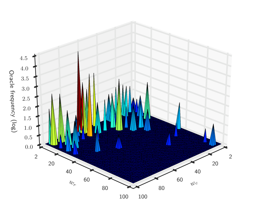
Figure 2: Oracle frequency counts for a subset of the workgroup sizes, $w_{c}\leq 100,w_{r}\leq 100$. There are 135 unique oracle workgroup sizes. The most common oracle workgroup size is $w_{(64\times 4)}$, optimal for 15% of scenarios.

Experimental results suggest that the problem is vendor — or at least device — specific. Figure 3 shows the ratio of refused test cases, grouped by device. We see many more refused parameters for test cases on Intel CPU devices than any other type, while no workgroup sizes were refused by the AMD GPU. The exact underlying cause for these refused parameters is unknown, but can likely by explained by inconsistencies or errors in specific OpenCL driver implementations. Note that the ratio of refused parameters decreases across the three generations of Nvidia GPUs: GTX 590 (2011), GTX 690 (2012), and GTX TITAN (2013). For now, it is imperative that any autotuning system is capable of adapting to these refused parameters by suggesting alternatives when they occur.

The baseline parameter is the workgroup size providing the best overall performance while being legal for all scenarios. Because of refused parameters, only a single workgroup size $w_{(4\times 4)}$ from the set of experimental results is found to have a legality of 100%, suggesting that an adaptive approach to setting workgroup size is necessary not just for the sake of maximising performance, but also for guaranteeing program execution. The utility of the baseline parameter is that it represents the best performance that can be achieved through static tuning of the workgroup size parameter; however, compared to the oracle workgroup size for each scenario, the baseline parameter achieves only 24% of the optimal performance.

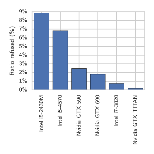
Figure 3: The ratio of test cases with refused workgroup sizes, grouped by OpenCL device ID. No parameters were refused by the AMD device.

7 Evaluation of Autotuning Methods

In this section we evaluate the effectiveness of the three proposed autotuning techniques for predicting performant workgroup sizes. For each autotuning technique, we partition the experimental data into training and testing sets. Three strategies for partitioning the data are used: the first is a 10-fold cross-validation; the second is to divide the data such that only data collected from synthetic benchmarks are used for training and only data collected from the real-world benchmarks are used for testing; the third strategy is to create leave-one-out partitions for each unique device, kernel, and dataset. For each combination of autotuning technique and testing dataset, we evaluate each of the workgroup sizes predicted for the testing data using the following metrics:

• time (real) — the time taken to make the autotuning prediction. This includes classification time and any communication overheads.

• accuracy (binary) — whether the predicted workgroup size is the true oracle, $w=\Omega(s)$.

• validity (binary) — whether the predicted workgroup size satisfies the workgroup size constraints constraints, $w<W_{\max}(s)$.

• refused (binary) — whether the predicted workgroup size is refused, $w\in W_{refused}(s)$.

• performance (real) — the performance of the predicted workgroup size relative to the oracle for that scenario.

• speedup (real) — the relative performance of the predicted workgroup size relative to the baseline workgroup size $w_{(4\times 4)}$.

The validty and refused metrics measure how often fallback strategies are required to select a legal workgroup size $w\in W_{legal}(s)$. This is only required for the classification approach to autotuning, since the process of selecting workgroup sizes using regressors respects workgroup size constraints.

7.1 Predicting Oracle Workgroup Size

Figure 4 shows the results when classifiers are trained using data from synthetic benchmarks and tested using real-world benchmarks. With the exception of the ZeroR, a dummy classifier which “predicts” only the baseline workgroup size $w_{\left(4\times 4\right)}$, the other classifiers achieve good speedups over the baseline, ranging from $4.61\times$ to $5.05\times$ when averaged across all test sets. The differences in speedups between classifiers is not significant, with the exception of SimpleLogistic, which performs poorly when trained with synthetic benchmarks and tested against real-world programs. This suggests the model over-fitting to features of the synthetic benchmarks which are not shared by the real-world tests. Of the three fallback handlers, NearestNeighbour provides the best performance, indicating that it successfully exploits structure in the optimisation space. In our evaluation, the largest number of iterations of a fallback handler required before selecting a legal workgroup size was 2.

7.2 Predicting with Regressors

Figure 5 shows a summary of results for autotuning using regressors to predict kernel runtimes (5(a)) and speedups (5(b)). Of the two regression techniques, predicting the speedup of workgroup sizes is much more successful than predicting the runtime. This is most likely caused by the inherent difficulty in predicting the runtime of arbitrary code, where dynamic factors such as flow control and loop bounds are not captured by the instruction counts which are used as features for the machine learning models. The average speedup achieved by predicting runtimes is $4.14\times$. For predicting speedups, the average is $5.57\times$, the highest of all of the autotuning techniques.

7.3 Autotuning Overheads

Comparing the classification times of Figures 4 and 5 shows that the prediction overhead of regressors is significantly greater than classifiers. This is because, while a classifier makes a single prediction, the number of predictions required of a regressor grows with the size of $W_{\max}(s)$, since classification with regression requires making predictions for all $w\in\left\{w|w<W_{\max}(s)\right\}$. The fastest classifier is J48, due to the it’s simplicity — it can be implemented as a sequence of nested if and else statements.

Figure 4: Autotuning performance using classifiers and synthetic benchmarks. Each classifier is trained on data collected from synthetic stencil applications, and tested for prediction quality using data from 6 real-world benchmarks. 95% confidence intervals are shown where appropriate.

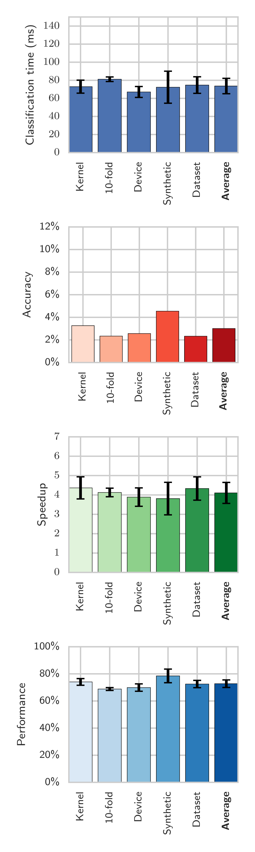
(a)

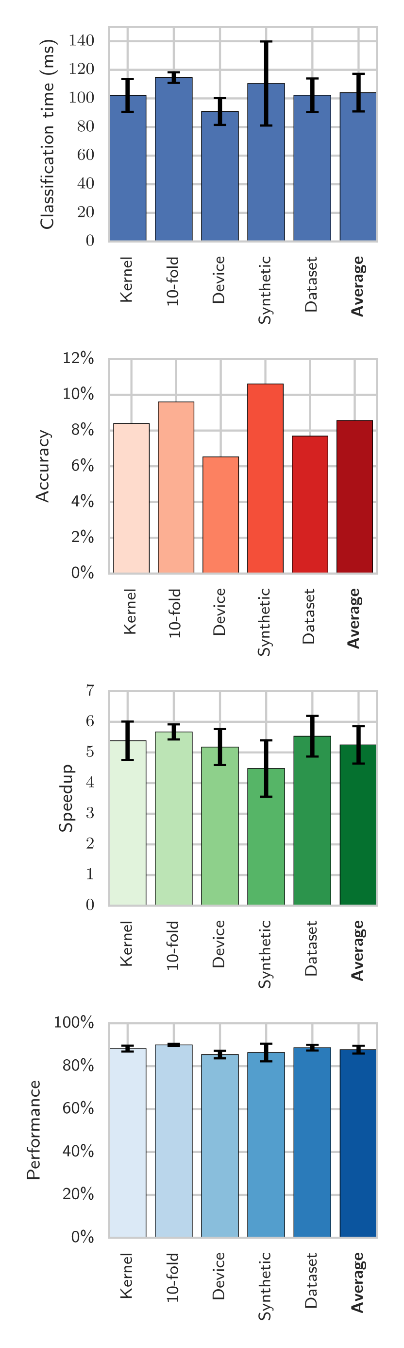
(b)

Figure 5: Autotuning performance for each type of test dataset using regressors to predict: (5(a)) kernel runtimes, and (5(b)) relative performance of workgroup sizes.

7.4 Comparison with Human Expert

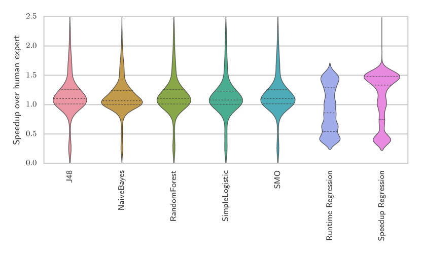
Figure 6: Violin plot of speedups over human expert, ignoring cases where the workgroup size selected by human experts is invalid. Classifiers are using NearestNeighbour fallback handlers. Horizontal dashed lines show the median, Q1, and Q3. Kernel Density Estimates show the distribution of results. The speedup axis is fixed to the range 0–2.5 to highlight the IQRs, which results in some outlier speedups > 2.5 being clipped.

In the original implementation of the SkelCL stencil pattern [7], Steuwer et al. selected a workgroup size of $w_{(32\times 4)}$ in an evaluation of 4 stencil operations on a Tesla S1070 system. In our evaluation of 429 combinations of kernel, architecture, and dataset, we found that this workgroup size is refused by 2.6% of scenarios, making it unsuitable for use as a baseline. However, if we remove the scenarios for which $w_{(32\times 4)}$ is not a legal workgroup size, we can directly compare the performance against the autotuning predictions.

Figure 6 plots the distributions and Interquartile Range (IQR) of all speedups over the human expert parameter for each autotuning technique. The distributions show consistent classification results for the five classification techniques, with the speedup at Q1 for all classifiers being $\geq 1.0\times$. The IQR for all classifiers is $<0.5$, but there are outliers with speedups both well below $1.0\times$ and well above $2.0\times$. In contrast, the speedups achieved using regressors to predict runtimes have a lower range, but also a lower median and a larger IQR. Clearly, this approach is the least effective of the evaluated autotuning techniques. Using regressors to predict relative performance is more successful, achieving the highest median speedup of all the techniques ($1.33\times$).

8 Related Work

Ganapathi et al. demonstrated early attempts at autotuning multicore stencil codes in [8], drawing upon the successes of statistical machine learning techniques in the compiler community. They use Kernel Canonical Correlation Analysis to build correlations between stencil features and optimisation parameters. Their use of KCCA restricts the scalability of their system, as the complexity of model building grows exponentially with the number of features. A code generator and autotuner for 3D Jacobi stencil codes is presented in [9], although their approach requires a full enumeration of the parameter space for each new program, and has no cross-program learning. Similarly, CLTune [10] is an autotuner which applies iterative search techniques to user-specified OpenCL parameters. The number of parallel mappers and reducers for MapReduce workloads is tuned in [11] using surrogate models rather than machine learning, although the optimisation space is not subject to the level of constraints that OpenCL workgroup size is. A generic OpenCL autotuner is presented in [12] which uses neural networks to predict good configurations of user-specified parameters, although the authors present only a preliminary evaluation using three benchmarks. Both systems require the user to specify parameters on a per-program basis. The autotuner presented in this work, embedded at the skeletal level, requires no user effort for new programs and is transparent to the user. A DSL and CUDA code generator for stencils is presented in [13]. Unlike the SkelCL stencil pattern, the generated stencil codes do not exploit fast local device memory. The automatic generation of synthetic benchmarks using parameterised template substitution is presented in [14]. The authors describe an application of their tool for generating OpenCL stencil kernels for machine learning, but do not report any performance results.

9 Conclusions

We present and compare novel methodologies for autotuning the workgroup size of stencil patterns using the established open source library SkelCL. These techniques achieve up to 94% of the maximum performance, while providing robust fallbacks in the presence of unexpected behaviour in OpenCL driver implementations. Of the three techniques proposed, predicting the relative performances of workgroup sizes using regressors provides the highest median speedup, whilst predicting the oracle workgroup size using decision tree classifiers adds the lowest runtime overhead. This presents a trade-off between classification time and training time that could be explored in future work using a hybrid of the classifier and regressor techniques presented in this paper.

In future work, we will extend the autotuner to accommodate additional OpenCL optimisation parameters and skeleton patterns. Feature selection can be evaluated using Principle Component Analysis, as well exploring the relationship between prediction accuracy and the number of synthetic benchmarks used. A promising avenue for further research is in the transition towards online machine learning which is enabled by using regressors to predict kernel runtimes. This could be combined with the use of adaptive sampling plans to minimise the number of observations required to distinguish bad from good parameter values, such as presented in [15]. Dynamic profiling can be used to increase the prediction accuracy of kernel runtimes by capturing the runtime behaviour of stencil kernels.

This work was supported by the UK Engineering and Physical Sciences Research Council under grants EP/L01503X/1 for the University of Edinburgh School of Informatics Centre for Doctoral Training in Pervasive Parallelism (http://pervasiveparallelism.inf.ed.ac.uk/), EP/H044752/1 (ALEA), and EP/M015793/1 (DIVIDEND).

References

- [1] Jeff Bolz, Ian Farmer, Eitan Grinspun and Peter Schroder “Sparse matrix solvers on the GPU: conjugate gradients and multigrid” In ACM TOG 22.3, 2003, pp. 917–924
- [2] John E. Stone, David Gohara and Guochun Shi “OpenCL: A Parallel Programming Standard for Heterogeneous Computing Systems” In Computing in Science & Engineering 12.3, 2010, pp. 66–73
- [3] Michel Steuwer, Philipp Kegel and Sergei Gorlatch “SkelCL - A Portable Skeleton Library for High-Level GPU Programming” In IPDPSW IEEE, 2011, pp. 1176–1182 DOI: 10.1109/IPDPS.2011.269
- [4] Jiawei Han, Micheline Kamber and Jian Pei “Data mining: concepts and techniques” Elsevier, 2011
- [5] Leo Breiman “Random forest” In Machine Learning 45.1, 2001, pp. 5–32 DOI: 10.1023/A:1010933404324
- [6] Intel Corporation “OpenCL* Optimization Guide”, 2012 URL: https://software.intel.com/sites/landingpage/opencl/optimization-guide/index.htm
- [7] Michel Steuwer, Michael Haidl, Stefan Breuer and Sergei Gorlatch “High-level programming of stencil computations on multi-GPU systems using the SkelCL library” In Parallel Processing Letters 24.03, 2014, pp. 1441005
- [8] Archana Ganapathi, Kaushik Datta, Armando Fox and David Patterson “A Case for Machine Learning to Optimize Multicore Performance” In HotPar, 2009
- [9] Yongpeng Zhang and Frank Mueller “Auto-generation and Auto-tuning of 3D Stencil Codes on GPU clusters” In CGO, 2012, pp. 155–164 DOI: 10.1109/TPDS.2012.160
- [10] Cedric Nugteren and Valeriu Codreanu “CLTune: A Generic Auto-Tuner for OpenCL Kernels” In MCSoC IEEE, 2015, pp. 195–202 DOI: 10.1109/MCSoC.2015.10
- [11] Travis Johnston, Mohammad Alsulmi, Pietro Cicotti and Michela Taufer “Performance Tuning of MapReduce Jobs Using Surrogate-Based Modeling” In ICCS, 2015, pp. 49–59
- [12] Thomas L. Falch and Anne C. Elster “Machine Learning Based Auto-tuning for Enhanced OpenCL Performance Portability” In IPDPSW IEEE, 2015, pp. 3–8 DOI: 10.1002/cpe
- [13] Shoaib Kamil, Cy Chan, Leonid Oliker, John Shall and Samuel Williams “An auto-tuning framework for parallel multicore stencil computations” In IPDPS, 2010 DOI: 10.1109/IPDPS.2010.5470421
- [14] Alton Chiu, Joseph Garvey and Tarek S Abdelrahman “Genesis: A Language for Generating Synthetic Training Programs for Machine Learning” In International Conference on Computing Frontiers ACM, 2015, pp. 8
- [15] Hugh Leather, Michael O’Boyle and Bruce Worton “Raced Profiles: Efficient Selection of Competing Compiler Optimizations” In ACM Sigplan Notices 44.7 ACM, 2009, pp. 50–59