Sympathetic cooling in a large ion crystal

Abstract

We analyze the dynamics and steady state of a linear ion array when some of the ions are continuously laser cooled. We calculate the ions’ local temperature measured by its position fluctuation under various trapping and cooling configurations, taking into account background heating due to the noisy environment. For a large system, we demonstrate that by arranging the cooling ions evenly in the array, one can suppress the overall heating considerably. We also investigate the effect of different cooling rates and find that the optimal cooling efficiency is achieved by an intermediate cooling rate. We discuss the relaxation time for the ions to approach the steady state, and show that with periodic arrangement of the cooling ions, the cooling efficiency does not scale down with the system size.

I Introduction

Trapped ions constitute one of the leading systems for implementation of quantum computation. Numerous advances have been achieved in this system, including realization of faithful quantum gates Sørensen and Mølmer (1999); Milburn et al. (2000); Sørensen and Mølmer (2000); Leibfried et al. (2003a); Myerson et al. (2008); Burrell et al. (2010); Harty et al. (2014), preparation of many-body quantum states Sackett et al. (2000); Leibfried et al. (2005); Häffner et al. (2005); Monz et al. (2011); Noguchi et al. (2012); Jurcevic et al. (2014); Lanyon et al. (2014); Northup (2015), and quantum teleportation Riebe et al. (2004); Olmschenk et al. (2009). There are also developments to scale up this system, based on either ion shuttling Kielpinski et al. (2002); Bowler et al. (2012); Walther et al. (2012) or quantum networks Duan et al. (2006); Moehring et al. (2007); Duan and Monroe (2010); Northup and Blatt (2014); Monroe et al. (2014); Hucul et al. (2015)).

In a typical ion trap, the ions are first Doppler cooled and form a crystal. Most of the quantum computation experiments use a one-dimensional ion crystal. The ions may be subjected to further sub-Doppler cooling, such as sideband cooling. However, the difficulty of sideband cooling scales up with the number of phonon modes, which increase with the number of ions Wineland et al. (1998); Leibfried et al. (2003b); Lin et al. (2009). It has been shown that in principle high-fidelity quantum computation can be achieved even at the Doppler temperature by employing the ions’ transverse phonon modes Zhu et al. (2006); Lin et al. (2009). In a real experimental setup, the ions are subject to substantial background heating. For long-time quantum computation, to have the ions constantly remain at a certain temperature, it requires sympathetic cooling Larson et al. (1986); Kielpinski et al. (2000), in which case a subset of ions (cooling ions) are continuously laser cooled, bringing down the temperature of other ions (the computational ions) through the heat propagation enabled by the Coulomb interaction in the ion crystal. Sympathetic cooling has been studied for small systems with a few ions Barrett et al. (2003); Home et al. (2009); Brown et al. (2011).

In this paper, we study the effectiveness of sympathetic cooling in a large one-dimensional ion crystal. Although in general temperature is not well defined for this system as it does not reach a thermal equilibrium state, as a relevant indicator for quantum computation, we measure the local “temperature” of the ions through their average position fluctuation (PF) $\delta x_{i}^{\xi}\equiv\sqrt{\langle x_{i}^{\xi 2}\rangle}$ (for the $i$th ion) with $\xi=x,y$ for the transverse phonon modes and $\xi=z$ for the the axial modes. This position thermal fluctuation is an important indicator for fidelity of quantum gates. We discuss two different arrangements of the cooling ions: edge cooling and periodic-node cooling. In the former case, the ions at the two edges of an ion array are continuously laser cooled. In the latter case, the cooling ions are distributed evenly and periodically in the ion chain. We show that the periodic-node cooling is much more effective than the edge cooling. For a large crystal, the edge cooling becomes very inefficient. We then discuss the nontrivial dependence of the local temperature of the computational ions on the cooling rate of the cooling ions. A large cooling rate does not necessarily lead to more efficient cooling of the computational ions. Instead, there is an intermediate optical cooling rate, in agreement with our previous observation Lin and Duan (2011). We finally investigate the time scale for the system to reach the steady state, which in general differs from the thermal equilibrium state Lin and Duan (2011).

This paper is organized as follows. In Sec. II, we present the Heisenberg-Langevin equations to describe the driven dynamics of a many-ion array and provide their formal exact solutions. In Sec. III, we discuss the motional steady states of the ions under background heating and continuous sympathetic cooling on the cooling ions. In Sec. IV, we study different cooling configurations and discuss the corresponding cooling efficiency. In Sec. V we investigate how the cooling performance of the sympathetic cooling depends on the laser cooling rate. In Sec. VI, we study the relaxation dynamics of the cooling process, and discuss the time scale of relaxation as well as its scaling with the system size. Finally, we summarize the major findings in Sec. VII.

II Formalism

Consider an ion string confined in an RF trap with an effective static potential $\mathcal{V}(\mathbf{r})=\frac{1}{2}m\omega_{x}^{2}(x^{2}+y^{2})+V(z)$. For a small crystal, the axial confinement is usually approximated by $V(z)=\frac{1}{2}m\omega_{z}^{2}z^{2}$ with $\omega_{z}\ll\omega_{x}$ so that the one dimensional alignment is stabilized. For a large crystal, the axial potential might take an anharmonic form Lin et al. (2009). Trapped ions have collective motion around their classical equilibrium positions. Assuming that each ion is coupled to its respective thermal bath (corresponding to either cooling or background heating), we describe the driven ion array by the following Heisenberg-Langevin equations:

$$\left\{\begin{array}[]{ccl}\dot{x}_{i}^{\xi}&=&p_{i}^{\xi}\\ \dot{p}_{i}^{\xi}&=&-\sum_{j}A_{ij}^{\xi}x_{j}^{\xi}-\gamma_{i}^{\xi}p_{i}^{\xi}+\sqrt{2\gamma_{i}^{\xi}}\zeta_{i}^{\xi}(t)\end{array}\right.,$$ (1)

where $i,j=1,...,N$ are ion indices, $\xi=x,y$,$z$ stands for the mode directions, and $A_{ii}^{\xi}=\beta_{i}^{\xi}-\sum_{j(\neq i)}\frac{C_{\xi}}{\left|z_{j}^{0}-z_{i}^{0}\right|^{3}},$ $A_{ij}^{\xi}=\frac{C_{\xi}}{\left|z_{j}^{0}-z_{i}^{0}\right|^{3}}(i\neq j)$ with $\beta_{i}^{x,y}=\omega_{x}^{2}$, $\beta_{i}^{z}=\partial^{2}V/\partial z_{i}^{2}$, $C_{x,y}=1$, $C_{z}=-2$, and $z_{i}^{0}$ denotes the $i$th ion’s axial equilibrium position. We take the ion spacing $d_{0}$ as the length unit, $e^{2}/d_{0}$ as the energy unit, and $\omega_{0}\equiv\sqrt{e^{2}/(md_{0}^{3})}$ as the frequency unit so that the quantities in Eq. (1) is dimensionless. For the convenience of discussion, we drop the superscript $\xi$. Since the transverse and axial modes are decoupled, the derivation simply applies to any direction. A random kick $\zeta_{i}(t)$ associated with the driving rate $\gamma_{i}$ can be expressed as $\zeta_{i}=-i\sum_{k}\sqrt{\frac{\omega_{k}}{2}}G_{ik}(b_{k}-b_{k}^{\dagger})$ (in units of $\sqrt{\hbar m\omega_{0}}$), where $G$ is the canonical transformation matrix which diagonalizes $A$, i.e. $G^{\top}AG=A^{D}$ is diagonalized, and $b_{k}$ is the bosonic field operator of the $k$th motional mode with frequency $\omega_{k}$. For a Markovian bath, $b_{k}(t)$ satisfies $\bigl{\langle}b_{k}^{\dagger}(t_{1})b_{k^{\prime}}(t_{2})\bigr{\rangle}=n_{k}^{B}(T)\delta_{kk^{\prime}}\delta(t_{1}-t_{2})$ with $n_{k}^{B}(T)\equiv\left[\exp(\omega_{k}/T)-1\right]^{-1}$ the phonon number of the $k$th mode for a given temperature $T$ (in units of $\hbar\omega_{0}/k_{B}$). It is then straightforward to show that the correlation of the driving force is given by $\bigl{\langle}\zeta_{i}(t)\zeta_{j}(t^{\prime})\bigr{\rangle}=\delta_{ij}\delta(t-t^{\prime})\sum_{k}\omega_{k}G_{ik}^{2}\bigl{(}n_{k}^{B}(T)+\frac{1}{2}\bigr{)}$. In our current case, where each ion couples to an independent reservoir $T_{i}$, it is reasonable to assume that the ion $i$ feels a local bath with $\bigl{\langle}\zeta_{i}(t)\zeta_{j}(t^{\prime})\bigr{\rangle}=\delta_{ij}\delta(t-t^{\prime})\Theta_{i}(T_{i})$ and $\Theta_{i}(T_{i})\equiv\sum_{k}\omega_{k}G_{ik}^{2}\bigl{(}n_{k}^{B}(T_{i})+\frac{1}{2}\bigr{)}$. The solution to Eq. (1) is given by $\mathbf{q}(t)=e^{-\Omega t}\mathbf{q}(0)+\int_{0}^{t}d\tau e^{\Omega(\tau-t)}\mathbf{\eta}(\tau)$, where $\mathbf{q}\equiv(x_{1},x_{2},...;p_{1},p_{2},...)^{\top}=\left[\begin{array}[]{c}\left\{x_{i}\right\}\\ \left\{p_{i}\right\}\end{array}\right]$, $\eta(t)\equiv\left[\begin{array}[]{c}\left\{0\right\}\\ \left\{\sqrt{2\gamma_{i}}\zeta_{i}\right\}\end{array}\right]$, and $\Omega\equiv\left[{\begin{array}[]{cc}{0}&{-I}\\ {\bigl{[}A_{ij}\bigr{]}}&\bigl{[}\gamma_{i}\delta_{ij}\bigr{]}\end{array}}\right]$ is a $2N\times 2N$ matrix which can be diagonalized as $\bigl{[}U^{-1}\Omega U\bigr{]}_{\alpha\beta}=\lambda_{\alpha}\delta_{\alpha\beta}$. We then obtain the variation of operators $x_{i}$ and $p_{i}$:

$$\bigl{\langle}q_{\mu}^{2}\bigr{\rangle} = \sum_{s=1}^{N}\sum_{\alpha,\beta=1}^{2N}U_{\mu\alpha}U_{\mu\beta}\Biggl{(}e^{-(\lambda_{\alpha}+\lambda_{\beta})t}\biggl{[}\bigl{\langle}x_{s}^{2}(0)\bigr{\rangle}U_{\beta s}^{-1}U_{\alpha s}^{-1}$$

$$+ \bigl{\langle}p_{s}^{2}(0)\bigr{\rangle}U_{\beta,s+N}^{-1}U_{\alpha,s+N}^{-1}\biggr{]}$$

$$+ \Bigl{(}1-e^{-(\lambda_{\alpha}+\lambda_{\beta})t}\Bigr{)}\frac{2\gamma_{s}\Theta_{s}}{\lambda_{\alpha}+\lambda_{\beta}}U_{\beta,s+N}^{-1}U_{\alpha,s+N}^{-1}\Biggr{)},$$

where $\mu=1,2,...,N$ correspond to $x$-operators, $\mu=N+1,N+2,...,2N$ correspond to $p$-operators.

For trapped ion quantum computing, the computational fidelity is determined by the ion PF $\delta x_{i}^{\xi}\equiv\sqrt{\bigl{\langle}x_{i}^{\xi 2}\bigr{\rangle}}$ (denoted by $\delta x_{i}$ and $\delta z_{i}$ for transverse and axial motion, respectively). When the quantum gate is operated by means of the transverse modes, the estimated infidelity is $\delta F_{i}^{x}\sim\pi^{2}\eta_{i}^{4}/4$ Sørensen and Mølmer (2000); Zhu et al. (2006); Lin et al. (2009), where the Lamb-Dicke parameter $\eta_{i}\sim\left|\Delta\mathbf{k}\right|\delta x_{i}$ with $\Delta\mathbf{k}\parallel\hat{x}$ the wavevector difference of the two Raman beams. Another possible source of error comes from the spatial non-uniformity of the laser intensity when a single beam addresses a specific ion; the ion’s axial motion results in variation of the actual Rabi frequency. This error is estimated by $\delta F_{i}^{z}\sim\pi^{2}(\delta z_{i}/w)^{4}/2$ given that the laser beam’s Rabi frequency is approximated by a Gaussian profile $\Omega(z)\propto e^{-((z-z_{i}^{0})/w)^{2}}$ with width $w$ Lin et al. (2009). Both of the gate errors are determined by the position thermal fluctuation $\delta x_{i}$ or $\delta z_{i}$ of the ions. So, in the following discussion we focus on the distribution of the ion position fluctuation $\delta x_{i}$ or $\delta z_{i}$ in the array.

III Steady-state distribution

III.1 Thermal equilibrium

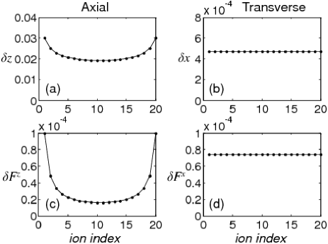
Figure 1: (a)(b) The thermal-equilibrium distributions of the averaged ion PF in units of $d_{0}$ and (c)(d) the associated computational infidelity corresponding to the axial and transverse motion at the Doppler temperature $k_{B}T_{D}/\hbar=2\pi\times 9.9$MHz for 20 ¹⁷¹Yb⁺ ions. Other parameters: $\omega_{x}=2\pi\times 5.1$MHz, $\omega_{z}=2\pi\times 34$kHz, $|\Delta\mathbf{k}|d_{0}=157$ with $d_{0}=10\mu$m, the minimal ion spacing in the middle of the chain.

We first look at the thermal-equilibrium distribution of the ion chain when the whole system is driven by a thermal field with a well-defined temperature. From $x_{i}=\alpha\sum_{k}G_{ik}\sqrt{\frac{1}{2\omega_{k}}}(a_{k}^{\dagger}+a_{k})$ where $\alpha\equiv\sqrt{\hbar/(m\omega_{0})}/d_{0}$ is the length conversion factor and $a_{k}$ ($a_{k}^{\dagger}$) is the annihilation (creation) operator of mode $k$, we obtain $\bigl{\langle}x_{i}^{2}\bigr{\rangle}=\alpha^{2}\sum_{k}\frac{G_{ik}^{2}}{\omega_{k}}\bigl{(}n_{k}^{B}(T)+\frac{1}{2}\bigr{)}=\alpha^{2}\sum_{k}\frac{G_{ik}^{2}}{2\omega_{k}}\coth\Bigl{(}\frac{\omega_{k}}{2T}\Bigr{)}$. In Fig. 1 we show the distribution of $\delta x_{i}$ and $\delta z_{i}$ in a harmonic trap for both the axial and transverse motion at the Doppler temperature $T_{D}$, and their contribution to the corresponding gate infidelities Lin et al. (2009). In this case, the axial fluctuation $\delta z_{i}$ varies in space, suggesting that the longitudinal motion of the whole ion chain is “more collective” and relies on the global geometry. Supposing that a single ion is subjected to a different temperature, its longitudinal movement does not directly reveal information of the temperature associated with the local bath because neighboring ions subjected to their own baths may interfere through collective modes. On the contrary, its transverse movement directly reflects the local temperature. This is because the axial and transverse modes are decoupled, and for each ion the energy scale set by the transverse confinement $\hbar\omega_{x}$ is dominant over other scales. Note that the diagonal terms of $A^{x}$ are more significant than the off-diagonal ones, meaning that the “local modes” defined by $x_{i}$ and $p_{i}^{x}$ can be discussed separately from those at different sites, with only small corrections due to inter-ion coupling. This is where the concept of a “local temperature” for a single ion starts to make sense. Such consideration has also motivated our investigation about the validity of classical thermal transportation for the trapped ion system Lin and Duan (2011). Each ion can then be approximated as an harmonic oscillator weakly coupled to others, whose “local” phonon occupation number is given by $n_{i}=\frac{\alpha^{-2}}{2}(\omega_{x}\langle x_{i}^{2}\rangle+\omega_{x}^{-1}\langle p_{i}^{x2}\rangle-1)\approx\alpha^{-2}\omega_{x}\langle x_{i}^{2}\rangle-\frac{1}{2}$. In the case shown in Fig. 1, PF$=10^{-3}d_{0}$ corresponds to $n_{i}=8.5$ with $\alpha=2.0\times 10^{-3}$.

III.2 Steady-state profile under sympathetic cooling

If different parts of the system make contact with reservoirs at different temperatures, as relevant for sympathetic cooling, the local temperature of the ions in the steady state will in general have a non-uniform spatial profile. In this section, we investigate this steady-state profile.

We first examine an example where the two edge portions of the ion chain are continuously laser cooled (we assume Doppler cooling, although the formalism also applies to other kinds of sympathetic cooling). The rest of the ion chain is driven by a hot bath corresponding to the background heating. According to Eq. (II), in the long-time limit a steady state should be reached, providing a time-invariant profile of the position fluctuation $\delta x_{i}$ or $\delta z_{i}$ over all the ions.

Figure 2: (Color online) The steady-state distributions of the ion PF in a harmonic trap under different background temperature for a given constant heating rate. As a comparison, the ideal (no background heating, $\gamma_{bg}=0$) curves are shown in red dotted lines.

To model the effect of background heating, we assume a small value for the background driving rate $\gamma_{bg}$ with respect to the associated environment temperature $T_{bg}$. The value of $T_{bg}$ is hard to quantify; the actual experimentally accessible parameter is the creation rate of phonons for a given motional mode $k$, that is, $\gamma_{bg}n_{k}^{B}\sim\gamma_{bg}T_{bg}/\omega_{k}$. To simplify our discussion, we treat the generated phonon numbers approximately the same around the range of all transverse (axial) modes. In other words, the background heating is now only characterized by $\kappa\equiv\gamma_{bg}T_{bg}$. Nevertheless, for a given value of $\kappa$ we still have the freedom to vary $T_{bg}$ (and hence $\gamma_{bg}$) while keeping $\kappa$ a constant parameter. As an example, we here consider an $N=20$ chain with $5$ ions on both ends as cooling ancillas. By denoting the set of the cooling ancillary ions by $C$ and rest of the chain by $H$, we take $T_{i}=T_{bg}$, $\gamma_{i}=\kappa/T_{bg}$ for $i\in H$ and $T_{i}=T_{D}$, $\gamma_{i}=0.1$ for $i\in C$. We then compare the resultant steady-state profile of $\delta x_{i}$ and $\delta z_{i}$ under various $T_{bg}$ in Fig. 2 with constant $\kappa=10^{-4}$, which amounts to a heating rate of about $60$ phonons per second per ion for the lowest axial mode of $2\pi\times 34$kHz. Note that in a real ion trap, a typical heating rate is about $100\sim 1000$ photons per second. As expected, the PF of the ancillary ions coincides with their supposed thermal-equilibrium values at the Doppler temperature $T_{D}$ while $\delta x_{i}$ and $\delta z_{i}$ show a hump in the middle part of the distribution due to the background heating. For $T_{bg}$ set to larger values, the hump grows but asymptotically converges to a fixed profile, providing an upper bound of the profile. This corresponds to the “worst” case with the largest contribution to the gate infidelity. In the following, we only show such upper bounds for all the circumstances and investigate the discrepancy between these bounds and the fluctuation profile at the Doppler temperature (corresponding to the perfectly cooled case).

IV Comparison of different cooling configurations

In this section, we compare the efficiency of sympathetic cooling under two cooling configurations: edge cooling and periodic-node cooling. For each case, we show the results under both harmonic and anharmonic axial traps. For a large ion crystal, the inhomogeneous ion spacing under a harmonic trap complicates the gate design and reduces its fidelity for quantum computation. To overcome this problem, as suggested in Lin et al. (2009), it is better to use anharmonic traps which can give equal or almost equal spacing for the ions in the chain. We consider two kinds of anharmonic trap: the one (called the uniform trap for simplicity of terminology) which gives perfect uniform spacing for the ions and the quartic trap with potential $V(z)=\frac{1}{2}\alpha_{2}z^{2}+\frac{1}{4}\alpha_{4}z^{4}$ which gives approximate uniform ion spacings. The parameters $\alpha_{2}$ and $\alpha_{4}$ in $V(z)$ are chosen to minimize the variation of the distribution of the ion spacings in the chain Lin et al. (2009).

IV.1 Edge cooling

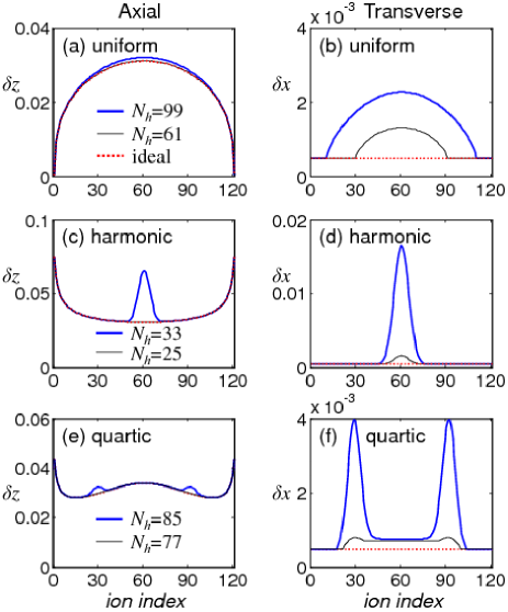
Figure 3: (Color online) The distributions of the axial and transverse PF (in units of $d_{0}$) for various trap geometries under the edge cooling: (a)(b) a uniform array, (c)(d) a harmonic trap, (e)(f) a quartic trap. $(N-N_{h})/2$ ions on each end of the ion chain are Doppler cooled with a driven rate $\gamma=0.1$. For the uniform array, the spacing is $d_{0}=10\mu$m; for the harmonic case, $\omega_{z}=2\pi\times 8.4$kHz and $\omega_{x}=2\pi\times 5.1$MHz, and for the quartic case $\omega_{2}\equiv\sqrt{|\alpha_{2}|/m}=2\pi\times 5$kHz and $|\alpha_{2}/e^{2}|^{2/3}(\alpha_{2}/\alpha_{4})=-6.2$ such that $\sum_{i=11}^{110}(z_{i+1}^{0}-z_{i}^{0})/100=d_{0}$. The background heating rate $\kappa=10^{-4}$ amounts to, for instance, generating $240$ phonons per second for the lowest harmonic mode $\omega_{z}$. Other parameters are the same as used in Fig. 1.

First, we show the result with the edge segments of the ions are Doppler cooled. Fig. 3 shows the final distributions of $\delta x_{i}$ and $\delta z_{i}$ under three different traps. As a comparison, the corresponding thermal-equilibrium profiles at $T=T_{D}$ are shown as red dotted curves. To consider how many ions can be cooled effectively through sympathetic cooling, we show the curves under different number $N_{h}\equiv n(H)$ of the computational ions which are subject to the background heating. The axial distribution is shown in Fig. 3(a), (c) and (e). In the uniform case, the curves almost coincide with the ideal thermal equilibrium one under the Doppler temperature, indicating that the system is almost perfectly cooled by sympathetic cooling. In our example with the system size $N=121$, the edge cooling for a uniform ion chain can afford $N_{h}$ up to $100$ ions, with the maximal $\delta z_{i}$ (occurring at the middle ion with $i=61$) increased by about $4\%$ compared with the ideal case. In the harmonic trap, the affordable $N_{h}$ is significantly reduced; the ion PF $\delta z_{i}$ grows very fast near the chain center as $N_{h}$ exceeds a certain value $(\sim 25)$. A considerable improvement can be found in the quartic case, which supports up to $N_{h}\sim 85$ ions with negligible discrepancy in the distribution. With even larger $N_{h}$, humps start to form on two sides instead of being at the chain center. As for the transverse motion, as shown in Fig. 3(b), (d), and (f), the cooling efficiency is in general more vulnerable than that of the axial motion. Because the transverse motion is typically more localized, the ancillary ions have vanishing influences on the ions of increasing distance. It can be observed that although $\delta x_{i}$ for the edge ions are fixed by the Doppler temperature, the ions away from the laser cooled ions soon get large $\delta x_{i}$. Therefore, we expect that it is inefficient to cool the transverse modes with the edge cooling.

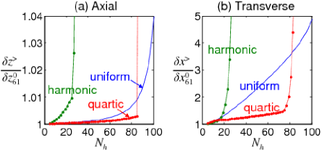
Figure 4: (Color online) The cooling efficiency (in terms of the normalized PF) as a function of the number of heat-driven ions for (a) the axial and (b) the transverse motion.

The dependence of the cooling efficiency on the number of computational ions $N_{h}$ is plotted in Fig. 4. To quantify the cooling efficiency, here we look at the maximal axial (transverse) position fluctuation $\delta z^{>}$ ($\delta x^{>}$) among all the ions belonging to $H$ normalized by the middle one’s fluctuation $\delta z_{m}^{0}$ ($\delta x_{m}^{0}$) at the Doppler temperature $T_{D}$ ($m=61$ for the system size $N=121$). With this definition, the normalized characteristic fluctuation approaches the unity when the system reaches the Doppler temperature. With this setup, the sympathetic cooling works better for the axial modes than the transverse ones in terms of the gate infidelities $\delta F^{z}$ and $\delta F^{x}$, which are proportional to $\bigl{(}\frac{\delta z^{>}}{\delta z_{61}^{0}}\bigr{)}^{4}$ and $\bigl{(}\frac{\delta x^{>}}{\delta x_{61}^{0}}\bigr{)}^{4}$, respectively. For instance, the infidelity $\delta F^{z}$ is roughly increased by $16\%$ for $\frac{\delta z^{>}}{\delta z_{61}^{0}}\sim 1.04$ but $\delta F^{x}$ is increased by $16$ times for $\frac{\delta x^{>}}{\delta x_{61}^{0}}\sim 2$. It is interesting to observe that for both the axial and transverse directions, the curves for the quartic trap rise more slowly than those for the uniform trap before they suddenly jump up around $N_{h}\sim 85$.

IV.2 Periodic-node cooling

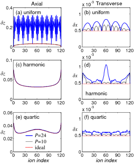
Figure 5: (Color online) The distributions of the axial and transverse PF (in units of $d_{0}$) under the periodic cooling for (a)(b) a uniform array, (c)(d) a harmonic trap, (e)(f) a quartic trap. The total number of ions $N=121$. All parameters are the same as in Fig. 3 except for the ancilla arrangement. The curve legend for all six panels is the same and is given in (e).

As discussed above for the edge cooling, if we impose an efficiency threshold, there must be a limit on $N_{h}$ beyond which the system cannot be effectively cooled. For long ion chains, therefore, a different spatial arrangement of the cooling ions must be considered. Here, we discuss an improved configuration where the ancillary cooling ions are distributed periodically and evenly in the ion chain. We investigate how the period (the number of computational ions between two adjacent cooling ions/nodes) influences the performance of sympathetic cooling. We still take the ion number $N=121$ as an example and only Doppler cool the $1$st, $(1+P)$th, $(1+2P)$th, …, $N$th ions with a period $P$ that factorizes $120$. In Fig. 5 we show the resultant distribution of $\delta x_{i}$ and $\delta z_{i}$ under three different trapping potentials. Unlike the edge cooling case, a uniform chain has no good performance under the periodic-node cooling. As the reason will be revealed later in Sec. V, this is because the cooling rate $\gamma=0.1$ is not an optimal choice. As for the axial motion in the harmonic and quartic cases shown in Fig. 5(c) and (e), the curves are almost identical to the ideal ones even with a large period $P=24$ (about $5\%$ of the ions are used for sympathetic cooling in this case). For the transverse direction shown in Fig. 5(b), (d), and (f), $\delta x_{i}$ is significantly suppressed compared to those under the edge cooling configuration. Although the detailed distribution depends on the trapping potential, the maximum $\delta x_{i}$ is no more than two ($1.25$) times of $\delta x_{i}$ for the ideal case under a large period $P=24$ ($P=10$).

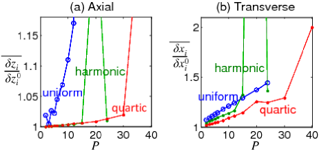
Figure 6: (Color online) The efficiency of the periodic cooling with different periods of ancilla arrangement for (a) the axial and (b) the transverse motion.

We plot the cooling efficiency against the period $P$ in Fig. 6. Here the efficiency is characterized by $\overline{\frac{\delta z_{i}}{\delta z_{i}^{0}}}\equiv\frac{1}{n(H)}\sum_{i\in H}\frac{\delta z_{i}}{\delta z_{i}^{0}}$ (similarly for $\overline{\frac{\delta x_{i}}{\delta x_{i}^{0}}}$). Note that in the uniform case, the efficiency becomes worse due to the improper choice of $\gamma=0.1$. For the axial modes shown in Fig. 6(a), the efficiency in the harmonic case is as good as that in the quartic case except at $P=20$, where the ion PF suddenly jumps out of the good range in the harmonic case. For the transverse modes (Fig. 6(a)), the three trap potentials do not show dramatic differences for $P<15$, but in general the quartic curve still shows the slowest increase in the ion PF as $P$ gets larger. The exception with a sudden jump of the PF at $P=20$ is somewhat related to a particular phonon eigenmode structure for the harmonic trap. Such a eigenmode happens to have a few nodal points coincident with the sites of cooling ions. Therefore this mode cannot be cooled effectively. This can be circumvented by arranging cooling ions asymmetrically with respect to the trap center. On the other hand, if some of the ions happen to be of large PF in one normal mode, cooling these ions effectively cools this mode. So it might be ideal to choose to cool those ions whose amplitudes are large in most of the eigenmodes.

V Influence of cooling rates

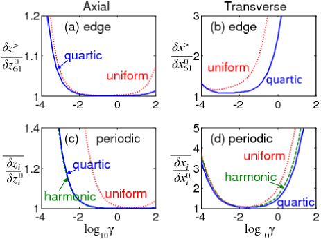
Figure 7: (Color online) The cooling efficiency for (a) the axial modes and (b) the transverse modes under edge cooling; (c) the axial modes and (d) the transverse modes under periodic-node cooling. The system size $N=121$. In (a) and (b), these curves correspond to $N_{h}=41$. In (c) and (d), the curves correspond to $P=10$. Other parameter are the same as previously discussed.

In this section, we discuss the significance of the driving rate $\gamma$ of the Doppler cooled ions. Intuitively, we would expect that the system can be cooled more efficiently when the driving rate $\gamma$ gets larger. Our calculation shows that this is however not the case. We study the efficiency with varied $\gamma$ under the same background heating rate $\kappa$. The efficiency characterized by the corresponding (normalized) position fluctuation is plotted in Fig. 7 as a function of $\gamma$. Surprisingly, for all the circumstances we consider, the ion position fluctuation first decreases as the driving rate rises in the small $\gamma$ regime, approaching to a minimum when $\gamma$ is moderate, and then increases again when $\gamma$ becomes strong. This suggests that the driving rate has an optimal window for cooling. The fact that the efficiency does not go better with strong cooling rates seems counter-intuitive in the first place. But this finding is consistent with our previous work Lin and Duan (2011). The reason is that, when the driving rate is larger than the inverse of the timescale needed for propagation, the ion is kicked from random directions so frequently that the effects of succeeding kicks cancel out before the first kick is about to “transfer” to its neighbors. If the rate matches the propagation timescale in order of magnitude, the cooling efficiency gets optimal.

Furthermore, these curves do not reach the minima at the same $\gamma$; the optimized cooling rate depends on the trapping potentials, cooling configurations, and which direction of the motion is considered. For the edge cooling (Fig. 7(a) and (b)), the most efficient window of $\gamma$ for cooling axial modes lies in the range from $0.1$ to $1$, both for the uniform and the quartic potentials. With the same rate, the (normalized) transverse PF becomes significantly larger than unity for these two geometries. For the periodic-node cooling (Fig. 7(c) and (d)), both the curves for the harmonic and the quartic potentials are nearly identical, with the optimal window lies in the range from $\gamma\sim 0.1$ to $10$ for the axial direction and from $\gamma\sim 0.02$ to $0.05$ for the transverse direction. By compromising the optimal windows for both the directions, $\gamma\simeq 0.1$ sounds a suitable choice.

VI Relaxation dynamics to the steady state

So far we have only discussed the steady-state solution to Eq. (II). In this section we discuss the relaxation time scale towards the steady state, which is also an important factor concerning the feasibility of employing the sympathetic cooling in experiments. To illustrate the general feature, we first calculate the dynamics of an $N=20$ ion chain in a harmonic trap under the edge cooling. We assume Doppler cooling is applied to $5$ ions on each end of the chain and the whole chain is initially in thermal equilibrium with temperature $T=2T_{D}$. We then plot the curves of $\delta x_{i}$ and $\delta z_{i}$ with $i=6$ (right next to the cooling ions) and $i=10$ (the middle ion) as indicators in Fig. 8(a) and (b). Note that for the axial motion the two solid lines have been coarse grained by a small time interval. This is because the actual profiles have very fast oscillations (see the insets of Fig. 8(a)). We also show the upper and lower envelopes of such oscillations by the dotted lines. The coarse-grained curves asymptotically approach constant values as time increases, along with the fast oscillations dying away gradually. We define a relaxation time $\tau_{R}$, beyond which the upper envelope falls within $1\%$ of the coarse-grained value. So we find $\tau_{R}/t_{0}\sim 10^{5}$ for the system to approach the steady state, where $t_{0}\equiv 2\pi/\omega_{0}$ ($\sim 7\mu$s for most of the cases discussed here). For the transverse direction, the amplitude of the fast oscillation is small, but it takes $\tau_{R}/t_{0}\sim 10^{6}$ to reach the steady state.

Now we consider the case with background heating at a rate $\kappa=\gamma_{bg}T_{bg}=10^{-4}$. Different curves corresponding to this case are plotted in dashed lines. Different $\gamma_{bg}$ change the final distribution of $\delta x_{i}$ and $\delta z_{i}$, but do not lead to significant variation of the relaxation time scale. Fig. 8(c) and (d) shows the snapshots of the distribution of $\delta x_{i}$ and $\delta z_{i}$ (coarse graining also applied to the axial mode) at different times. The cooling ions immediately reach their steady states (in a short time scale $\gamma^{-1}$ which is not visible from the curve). The cooling then starts to propagate to the inner part of the ion chain.

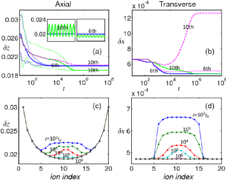
Figure 8: (Color online) (a)(b) The temporal profiles of the ion PF for the $6$th (blue curves) and $10$th (green curves) ions without considering background heating. In (a), two solid lines represent coarse-grained values since the actual profiles contain fast oscillations as seen in the two insets at $t=10^{4}t_{0}$ (left) and $t=10^{5}t_{0}$ (right), respectively. The coarse graining interval is $\Delta t/t_{0}=20$. Note that in both insets the time span is $\Delta t^{\prime}/t_{0}=10$, and the wavy (green) behavior belongs to the $10$th ion while the PF of the $6$th ion stays nearly a constant (blue). To show the effect of background heating, the PF profile of the $10$th ion is also plotted for comparison (with $\kappa=10^{-4}$). That of the $6$th ion is not explicitly shown because it is almost identical to the blue solid (no-heating) curve. In (b), the fast oscillation amplitude is in the order of $10^{-9}d_{0}$ so the dotted curves appear to be on top of the solid ones. A thick and a thin (magenta) dotted lines representing the $10$th and $6$th ions, respectively, with background heating are also shown for comparison. (c)(d) The snapshots of the time-averaged distributions. The relevant parameters are the same as Fig. 2.

Previous discussion has shown that the relaxation time of edge cooling is still quite long (0.1 to 1 second). We then turn to the more efficient periodic-node cooling for a large ion chain. We here consider a quartic trap and examine the relaxation time $\tau_{R}$ as a function of the period $P$. As expected, Fig. 9(a) shows that $\tau_{R}$ is in general an increasing function with $P$. For an $N=121$ chain, we find the time scale can be controlled within $\tau_{R}/t_{0}\sim 10^{4}$ (tens of milliseconds) while the axial relaxation takes roughly $10$ times shorter than the transverse one. These results show a timescale comparable to usual Doppler cooling (of order of a few milliseconds). If the background heating is included, the transverse curve drops slightly but the axial curve is hardly affected. As more ions are added into the system, it is important to make sure that the relaxation time does not scale up too fast with $N$. We show in Fig. 9(b) the scaling curves of $\tau_{R}$ with increasing $N$ by fixing $P=10$. The axial relaxation time tends to decrease as the system size increases and meets a lower bound in the large $N$ limit. On the contrary, the transverse relaxation time appears to be independent of $N$. This is because the transverse motion tends to involve only nearby ions. So a longer chain is nothing but a simple repetition of segments of a size $P$.

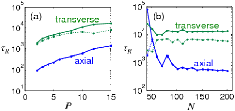
Figure 9: (Color online) The relaxation time $\tau_{R}$ as a function of (a) the period $P$ in the periodic-node cooling for $N=121$, and (b) the total length $N$ of the ion chain for a given $P=10$. The solid curves correspond to no background heating cases and the dotted lines correspond to background heating cases with $\kappa=10^{-4}$. For (a), the relevant parameters are the same as Fig. 5. For chains of different sizes in (b), the quartic trap is determined by minimizing $\sum_{i=16}^{N-16}(z_{i+1}^{0}-z_{i}^{0})^{2}/(N-31)$ and setting $\sum_{i=16}^{N-16}(z_{i+1}^{0}-z_{i}^{0})/(N-31)=d_{0}$.

VII Conclusion

To conclude, we have presented a detailed investigation on the sympathetic cooling in a large ion chain. Many findings discovered in this paper are instructional for experimental implementation. First, a steady state can be reached for a system subject to constant background heating under continuous sympathetic cooling. By arranging cooling ancillary ions in different ways, the cooling performance can be improved and optimized. In our calculation, although the transverse motion is relatively harder to be cooled than the axial one, by inserting ancillary ions evenly over the chain it can be cooled down to a satisfactory level. We have studied the effect of cooling rates and found the optimal window of the cooling rates. We have also discussed the relaxation dynamics and showed that the required time scale is within the reach of experiments.

References

- Sørensen and Mølmer (1999) A. Sørensen and K. Mølmer, Phys. Rev. Lett. 82, 1971 (1999).
- Milburn et al. (2000) G. Milburn, S. Schneider, and D. James, Fortschritte der Physik 48, 801 (2000).
- Sørensen and Mølmer (2000) A. Sørensen and K. Mølmer, Phys. Rev. A 62, 022311 (2000).
- Leibfried et al. (2003a) D. Leibfried, B. DeMarco, V. Meyer, D. Lucas, M. Barrett, J. Britton, W. M. Itano, B. Jelenković, C. Langer, T. Rosenband, et al., Nature 422, 412 (2003a).
- Myerson et al. (2008) A. H. Myerson, D. J. Szwer, S. C. Webster, D. T. C. Allcock, M. J. Curtis, G. Imreh, J. A. Sherman, D. N. Stacey, A. M. Steane, and D. M. Lucas, Phys. Rev. Lett. 100, 200502 (2008).
- Burrell et al. (2010) A. H. Burrell, D. J. Szwer, S. C. Webster, and D. M. Lucas, Phys. Rev. A 81, 040302 (2010).
- Harty et al. (2014) T. P. Harty, D. T. C. Allcock, C. J. Ballance, L. Guidoni, H. A. Janacek, N. M. Linke, D. N. Stacey, and D. M. Lucas, Phys. Rev. Lett. 113, 220501 (2014).
- Sackett et al. (2000) C. A. Sackett, D. Kielpinski, B. E. King, C. Langer, V. Meyer, C. J. Myatt, M. Rowe, Q. A. Turchette, W. M. Itano, D. J. Wineland, et al., Nature 404, 256 (2000), ISSN 0028-0836.
- Leibfried et al. (2005) D. Leibfried, E. Knill, S. Seidelin, J. Britton, R. B. Blakestad, J. Chiaverini, D. B. Hume, W. M. Itano, J. D. Jost, C. Langer, et al., Nature 438, 639 (2005), ISSN 0028-0836.
- Häffner et al. (2005) H. Häffner, W. Hänsel, C. F. Roos, J. Benhelm, D. Chek-al-kar, M. Chwalla, T. Körber, U. D. Rapol, M. Riebe, P. O. Schmidt, et al., Nature 438, 643 (2005), ISSN 0028-0836.
- Monz et al. (2011) T. Monz, P. Schindler, J. T. Barreiro, M. Chwalla, D. Nigg, W. A. Coish, M. Harlander, W. Hänsel, M. Hennrich, and R. Blatt, Phys. Rev. Lett. 106, 130506 (2011).
- Noguchi et al. (2012) A. Noguchi, K. Toyoda, and S. Urabe, Phys. Rev. Lett. 109, 260502 (2012).
- Jurcevic et al. (2014) P. Jurcevic, B. P. Lanyon, P. Hauke, C. Hempel, P. Zoller, R. Blatt, and C. F. Roos, Nature 511, 202 (2014).
- Lanyon et al. (2014) B. P. Lanyon, M. Zwerger, P. Jurcevic, C. Hempel, W. Dür, H. J. Briegel, R. Blatt, and C. F. Roos, Phys. Rev. Lett. 112, 100403 (2014).
- Northup (2015) T. Northup, Nature 521, 295 (2015), ISSN 0028-0836.
- Riebe et al. (2004) M. Riebe, H. Häffner, C. F. Roos, W. Hänsel, J. Benhelm, G. P. T. Lancaster, T. W. Körber, C. Becher, F. Schmidt-Kaler, D. F. V. James, et al., Nature 429, 734 (2004), ISSN 0028-0836.
- Olmschenk et al. (2009) S. Olmschenk, D. N. Matsukevich, P. Maunz, D. Hayes, L.-M. Duan, and C. Monroe, Science 323, 486 (2009).
- Kielpinski et al. (2002) D. Kielpinski, C. Monroe, and D. J. Wineland, Nature 417, 709 (2002).
- Bowler et al. (2012) R. Bowler, J. Gaebler, Y. Lin, T. R. Tan, D. Hanneke, J. D. Jost, J. P. Home, D. Leibfried, and D. J. Wineland, Phys. Rev. Lett. 109, 080502 (2012).
- Walther et al. (2012) A. Walther, F. Ziesel, T. Ruster, S. T. Dawkins, K. Ott, M. Hettrich, K. Singer, F. Schmidt-Kaler, and U. Poschinger, Phys. Rev. Lett. 109, 080501 (2012).
- Duan et al. (2006) L.-M. Duan, M. J. Madsen, D. L. Moehring, P. Maunz, R. N. Kohn, and C. Monroe, Phys. Rev. A 73, 062324 (2006).
- Moehring et al. (2007) D. L. Moehring, P. Maunz, S. Olmschenk, K. C. Younge, D. N. Matsukevich, L.-M. Duan, and C. Monroe, Nature 449, 68 (2007), ISSN 0028-0836.
- Duan and Monroe (2010) L.-M. Duan and C. Monroe, Rev. Mod. Phys. 82, 1209 (2010).
- Northup and Blatt (2014) T. E. Northup and R. Blatt, Nat Photon 8, 356 (2014).
- Monroe et al. (2014) C. Monroe, R. Raussendorf, A. Ruthven, K. R. Brown, P. Maunz, L.-M. Duan, and J. Kim, Phys. Rev. A 89, 022317 (2014).
- Hucul et al. (2015) D. Hucul, I. V. Inlek, G. Vittorini, C. Crocker, S. Debnath, S. M. Clark, and C. Monroe, Nat Phys 11, 37 (2015).
- Wineland et al. (1998) D. Wineland, C. Monroe, W. M. Itano, D. Leibfried, B. E. King, and D. M. Meekhof, J. Res. Natl. Inst. Stand. Tech. 103, 259 (1998).
- Leibfried et al. (2003b) D. Leibfried, R. Blatt, C. Monroe, and D. Wineland, Rev. Mod. Phys. 75, 281 (2003b).
- Lin et al. (2009) G.-D. Lin, S.-L. Zhu, R. Islam, K. Kim, M.-S. Chang, S. Korenblit, C. Monroe, and L.-M. Duan, Europhys. Lett. 86, 60004 (5pp) (2009).
- Zhu et al. (2006) S.-L. Zhu, C. Monroe, and L.-M. Duan, Phys. Rev. Lett. 97, 050505 (2006).
- Larson et al. (1986) D. J. Larson, J. C. Bergquist, J. J. Bollinger, W. M. Itano, and D. J. Wineland, Phys. Rev. Lett. 57, 70 (1986).
- Kielpinski et al. (2000) D. Kielpinski, B. E. King, C. J. Myatt, C. A. Sackett, Q. A. Turchette, W. M. Itano, C. Monroe, D. J. Wineland, and W. H. Zurek, Phys. Rev. A 61, 032310 (2000).
- Barrett et al. (2003) M. D. Barrett, B. DeMarco, T. Schaetz, V. Meyer, D. Leibfried, J. Britton, J. Chiaverini, W. M. Itano, B. Jelenković, J. D. Jost, et al., Phys. Rev. A 68, 042302 (2003).
- Home et al. (2009) J. P. Home, M. J. McDonnell, D. J. Szwer, B. C. Keitch, D. M. Lucas, D. N. Stacey, and A. M. Steane, Phys. Rev. A 79, 050305 (2009).
- Brown et al. (2011) K. R. Brown, C. Ospelkaus, Y. Colombe, A. C. Wilson, D. Leibfried, and D. J. Wineland, Nature 471, 196 (2011).
- Lin and Duan (2011) G.-D. Lin and L.-M. Duan, New Journal of Physics 13, 075015 (2011).