The Coriolis field

Abstract

We present a pedagogical discussion of the Coriolis field, emphasizing its not-so-well-understood aspects. We show that this field satisfies the field equations of the so-called Newton-Cartan theory, a generalization of Newtonian gravity that is covariant under changes of arbitrarily rotating and accelerated frames. Examples of solutions of this theory are given, including the Newtonian analogue of the Gödel universe. We discuss how to detect the Coriolis field by its effect on gyroscopes, of which the gyrocompass is an example. Finally, using a similar framework, we discuss the Coriolis field generated by mass currents in general relativity, and its measurement by the Gravity Probe B and LAGEOS/LARES experiments.

I Red Planet and the principle of equivalence

In the movie Red Planet (2000), a spaceship traveling to Mars simulates gravity by using a spinning wheel.wheel The astronauts living inside the wheel are pushed against the outer wall, which they perceive as the floor, by the centrifugal force. At some point during the movie a power failure causes the wheel to stop spinning, leading to a zero gravity environment. This event provides the necessary dramatic setting for commander Kate Bowman to save the day, including explosively decompressing the wheel to extinguish a zero-$g$ fire. When she gets the main power back online the wheel starts spinning again, and everything—including her—immediately falls to the floor. But as noted on the popular website “Bad Astronomy,”BA this is not what would happen in such a situation. Instead, imagine commander Bowman floating motionless (with respect to some inertial frame, say the rest frame of the distant stars) inside the wheel (see Fig. 1) and assume, for simplicity, that there is no air inside the spaceship. From the point of view of the star fixed inertial frame it is clear that, no matter how fast the wheel spins, she will feel no force and will continue floating motionless inside the wheel.

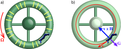
Figure 1: Commander Bowman floating inside the rotating wheel as seen: (a) in an inertial frame; (b) in a frame co-rotating with the wheel. From the point of view of the inertial frame, she is freely falling and remains stationary. From the point of view of the wheel’s frame, she is in a circular orbit under the action of two forces: a centrifugal force $m{\bf G}$ (that pushes her outwards), and a centripetal Coriolis force $m{\bf v}\times{\bf H}=-2m{\bf G}$, with twice the magnitude of the centrifugal force (that pushes her inwards).

If we take the perspective of the wheel’s (rotating) frame and interpret the centrifugal (inertial) force as a gravitational field the situation looks very strange: commander Bowman is subject to a gravitational force and yet she does not fall. After a moment’s thought, one realizes that such a thing happens all the time in “real” gravitational fields: it is called being in orbit. In the wheel’s rotating frame, Commander Bowman is moving along a circle with the right velocity so that she does not fall. However, the gravitational field (centrifugal force) points outward, away from the center of her trajectory. So how can she be in orbit in this gravitational field? Something is surely missing.

II Non-relativistic inertial forces: Newton-Cartan theory

The missing ingredient is, of course, the Coriolis force; it is this velocity-dependent force that pushes commander Bowman towards the center of her orbit. This reminds us that Einstein’s equivalence principle,Einstein when applied to arbitrarily accelerated and rotating frames, requires the introduction of a magnetic-like Coriolis field.

In this section we will revisit the problem of the inertial forces arising in an arbitrarily accelerated and rotating (rigid) frame, and obtain the so-called Newton-Cartan equations, which will be useful in our further study of the Coriolis field in the next sections. Let ${\bf x}(t)$ be the position vector of a particle of mass $m$ in an inertial frame $S$ (say, the rest frame of the distant stars), and let ${\bf r}(t)$ be the position vector of the same particle in an accelerated and rotating frame $S^{\prime}$ (for example, the wheel’s frame). If we denote the position of the origin of $S^{\prime}$ in $S$ by ${\bf x}_{0}(t)$ then

$${\bf x}(t)=R(t){\bf r}(t)+{\bf x}_{0}(t)\ ,$$ (1)

for some time-dependent rotation matrix $R(t)$. In the example above, for instance, ${\bf x}_{0}(t)$ represents the position of the center of the wheel and

$$R(t)=\left(\begin{matrix}\cos(\Omega t)&-\sin(\Omega t)&0\\ \sin(\Omega t)&\cos(\Omega t)&0\\ 0&0&1\end{matrix}\right),$$ (2)

where we have assumed that the wheel is rotating around the $z$-axis with constant angular velocity $\Omega$.

If we assume that the particle is subject to a gravitational field ${\bf g}$ plus a nongravitational force $\mathbf{f}$, then the particle’s equation of motion will be

$$m\ddot{{\bf x}}=m{\bf g}+\mathbf{f}\ ,$$ (3)

where dots represent time derivatives. As usual, we take the gravitational field to satisfy

$$\nabla\times{\bf g}={\bf 0},\qquad\nabla\cdot{\bf g}=-4\pi G\rho\ ,$$ (4)

where $G$ is Newton’s constant and $\rho$ is the mass density of the matter generating the field.

To write the equation of motion in the frame $S^{\prime}$, we note that

$$\dot{{\bf x}}=R\dot{{\bf r}}+\dot{R}{\bf r}+\dot{{\bf x}}_{0}\ .$$ (5)

Since $R$ is a rotation matrix, its inverse coincides with its transpose: $R^{T}=R^{-1}$. Hence

$$R^{T}R=I\Rightarrow\dot{R}^{T}R+R^{T}\dot{R}=0\Leftrightarrow R^{T}\dot{R}=-\left(R^{T}\dot{R}\right)^{T},$$ (6)

that is, the matrix $A=R^{T}\dot{R}$ is antisymmetric (and thus it has only three independent components, say $\Omega^{1}$, $\Omega^{2}$ and $\Omega^{3}$). Consequently, we can write $A_{ij}=\epsilon_{ikj}\Omega^{k}$, where $\epsilon_{ijk}$ is the Levi-Civita alternating symbol, which means $A{\bf r}={\bf\Omega}\times{\bf r}$ and thus

$$\dot{R}{\bf r}=RA{\bf r}=R({\bf\Omega}\times{\bf r})\ .$$ (7)

Note from Eqs. (5) and (7) that the velocity vector of a particle at rest in $S^{\prime}$ is

$$\dot{{\bf x}}=R({\bf\Omega}\times{\bf r})+\dot{{\bf x}}_{0}=(R{\bf\Omega})\times(R{\bf r})+\dot{{\bf x}}_{0}\ ,$$ (8)

where in the last equality we used the fact that rotations preserve cross products, since they preserve lengths, angles, and orientations. This equation tells us that ${\bf\Omega}$ is the angular velocity of $S^{\prime}$ with respect to $S$, expressed in $S^{\prime}$ (that is, the angular velocity in $S$ is $R{\bf\Omega}$). Note that since $R=R(t)$ depends only on time, then so does ${\bf\Omega}={\bf\Omega}(t)$.

For an arbitrarily moving particle we have, from Eqs. (5) and (7),

$$\dot{{\bf x}}=R\dot{{\bf r}}+R({\bf\Omega}\times{\bf r})+\dot{{\bf x}}_{0}$$ (9)

and

$$\ddot{{\bf x}}=R\ddot{{\bf r}}+2R({\bf\Omega}\times\dot{{\bf r}})+R\left[{\bf\Omega}\times({\bf\Omega}\times{\bf r})\right]+R(\dot{{\bf\Omega}}\times{\bf r})+\ddot{{\bf x}}_{0}\ .$$ (10)

The equation of motion in $S^{\prime}$ is then

$$m\ddot{{\bf r}}=m{\bf G}+m\dot{{\bf r}}\times{\bf H}+{\bf F}\ ,$$ (11)

where ${\bf F}=R^{-1}{\bf f}$ is the nongravitational force expressed in $S^{\prime}$, and we have defined the field

$${\bf G}=R^{-1}({\bf g}-\ddot{{\bf x}}_{0})-{\bf\Omega}\times({\bf\Omega}\times{\bf r})-\dot{{\bf\Omega}}\times{\bf r}\ ,$$ (12)

and the Coriolis field

$${\bf H}=2{\bf\Omega}\ .$$ (13)

In other words, to explain the motion of the particle in the frame $S^{\prime}$ we need two fields: a field ${\bf G}$, consisting of the preexisting gravitational field plus inertial terms,inertialterms and a Coriolis field ${\bf H}$, which is twice the angular velocity of $S^{\prime}$ and which gives rise to the magnetic-like velocity-dependent Coriolis force $m\dot{{\bf r}}\times{\bf H}$.

Note from Eq. (11) that ${\bf G}$ is minus the nongravitational force per unit mass acting on observers at rest in $S^{\prime}$; this is exactly what a weighing scale placed in $S^{\prime}$ will measure. Moreover, Eq. (8) implies that observers at rest in $S^{\prime}$ are seen to move in $S$ along the velocity field

$${\bf v}({\bf x},t) =(R{\bf\Omega})\times(R{\bf r})+\dot{{\bf x}}_{0}$$

$$=(R{\bf\Omega})\times({\bf x}-{\bf x}_{0})+\dot{{\bf x}}_{0}\ ,$$ (14)

whose vorticity (in $S$) is

$${\boldsymbol{\omega}}\equiv\frac{1}{2}\nabla\times{\bf v}=\frac{1}{2}\nabla\times\left[(R{\bf\Omega})\times{\bf x}\right]=R{\bf\Omega}\ .$$ (15)

Here we have used the vector identity

$$\nabla\times(\mathbf{a}\times\mathbf{b})=\mathbf{a}(\nabla\cdot\mathbf{b})-(\mathbf{a}\cdot\nabla)\mathbf{b}\ ,$$ (16)

which holds for a spatially constant vector $\mathbf{a}$, together with the identities $\nabla\cdot{\bf x}=3$ and $(\mathbf{a}\cdot\nabla)\mathbf{x}=\mathbf{a}$. Thus, we see that ${\bf H}=2{\bf\Omega}=R^{-1}(2{\boldsymbol{\omega}})$ is twice the vorticity of the observers at rest in $S^{\prime}$ (as seen in $S$ and expressed in $S^{\prime}$). These observations will be important for the comparison with the relativistic inertial forces in Sec. III.

Since the Coriolis field does not depend on the space coordinates, as ${\bf H}=2{\bf\Omega}(t)$, it trivially satisfies

$$\nabla\times{\bf H}={\bf 0}\ ,\qquad\nabla\cdot{\bf H}=0\ .$$ (17)

Conversely, if ${\bf H}$ satisfies these equations and is spatially constant at infinity then it must be spatially constant everywhere. This fact can be seen by noting that $\nabla\times\bf{H}=0$ implies that $\bf{H}=\nabla\psi$, for some scalar function $\psi$; then $\nabla\cdot\bf{H}=0$ implies $\nabla^{2}\psi=0$, i.e, $\bf{H}$ is the gradient of a solution of the Laplace equation. By virtue of the Green theorem (see, e.g., Secs. 1.8-1.9 of Ref. Jackson, ), such a solution is unique (up to a constant) if boundary conditions for its gradient are given at infinity. Therefore it must be the solution whose gradient, that is, ${\bf H}$, is spatially constant.

If we take the curl of Eq. (12) we obtain

$$\nabla\times{\bf G}=-2\dot{{\bf\Omega}}=-\frac{\partial{\bf H}}{\partial t}\,.$$ (18)

To obtain this result, we: (i) used the covariance of this differential operator under rotations,Cox so that $\nabla\times(R^{-1}{\bf g})=R^{-1}(\nabla\times{\bf g})={\bf 0}$; (ii) noted, from elementary vector identities, that ${\bf\Omega}\times({\bf\Omega}\times{\bf r})=({\bf\Omega}\cdot\mathbf{r}){\bf\Omega}-\Omega^{2}\mathbf{r}$ and $\nabla\times\left[({\bf\Omega}\cdot\mathbf{r}){\bf\Omega}\right]=\nabla({\bf\Omega}\cdot\mathbf{r})\times{\bf\Omega}={\bf 0}$; and (iii) used Eq. (16) to obtain $\nabla\times(\dot{{\bf\Omega}}\times{\bf r})=2\dot{{\bf\Omega}}$.

Similarly, taking the divergence of Eq. (12) yields

$$\nabla\cdot{\bf G}=\nabla\cdot{\bf g}+2{\bf\Omega}^{2}=-4\pi G\rho+\frac{1}{2}{\bf H}^{2}\,,$$ (19)

where we again used the invariance of this differential operator under rotations,Cox $\nabla\cdot(R^{-1}{\bf g})=\nabla\cdot{\bf g}$, and noted that $\nabla\cdot(\dot{{\bf\Omega}}\times{\bf r})=0$ from the vector identity $\nabla\cdot(\mathbf{a}\times\mathbf{b})=\mathbf{b}\cdot(\nabla\times\mathbf{a})-\mathbf{a}\cdot(\nabla\times\mathbf{b})$. Note the similarity of Eqs. (17)–(19) with Maxwell’s equations, apart from the absence of source and displacement currents in the equation for $\nabla\times{\bf H}$ and the nonlinear term in the equation for $\nabla\cdot{\bf G}$.

If there are no nongravitational forces acting on the particle, then its mass $m$ drops out of Eq. (11):

$$\ddot{{\bf r}}={\bf G}+\dot{{\bf r}}\times{\bf H}\ .$$ (20)

This equation, together with the field equations

$$\begin{cases}{\displaystyle\nabla\times{\bf G}=-\frac{\partial{\bf H}}{\partial t}}\\ \nabla\times{\bf H}={\bf 0}\\ {\displaystyle\nabla\cdot{\bf G}=-4\pi G\rho+\frac{1}{2}{\bf H}^{2}}\\ \nabla\cdot{\bf H}=0\;,\end{cases}$$ (21)

form the basis of the so-called Newton-Cartan theory of gravity.Newton-Cartan This theory is a generalization of the usual Newtonian gravity theory that is covariant under changes of rigid frame, in the sense that Eqs. (20) and (21) are invariant under such changes (just like the Maxwell equations and the Lorentz force law are invariant under changes of inertial frame). In this theory, inertial frames are thus no longer privileged—all inertial forces are explained as a combination of the fields ${\bf G}$ and ${\bf H}$. Unsurprisingly, it is the (singular) limit of general relativity as the speed of light tends to infinity.R89 ; D90 ; E91 ; E97

The Newton-Cartan theory is, however, more general than the usual Newtonian theory because it admits solutions with spatially varying Coriolis fields, which do not correspond to a Newtonian field as seen in an accelerated and rotating frame. Such non-Newtonian solutions can be excluded by imposing appropriate boundary conditions at infinity, and will not be considered here.

II.1 Uniform rotation

The uniformly rotating frame provides a particular solution of the Newton-Cartan field equations (21) with $\rho=0$, given by

$$\begin{cases}{\bf G}=\Omega^{2}r\,{\bf e}_{r}\\ {\bf H}=2\Omega\,{\bf e}_{z}\,,\end{cases}$$ (22)

where $\Omega$ is the magnitude of the constant angular velocity, $(r,\theta,z)$ are the obvious cylindrical coordinates, and ${\bf e}_{r},{\bf e}_{\theta}$, and ${\bf e}_{z}$ are the corresponding unit vectors. The condition for a particle to be in circular orbit, with tangential velocity $\dot{\mathbf{r}}={\bf v}=v\,{\bf e}_{\theta},$ is that the centripetal acceleration

$$\ddot{\mathbf{r}}=v\,\dot{{\bf e}}_{\theta}=-\frac{v^{2}}{r}{\bf e}_{r}$$ (23)

equals the gravitational acceleration in Eq. (20):

$$-\frac{v^{2}}{r}{\bf e}_{r}={\bf G}+{\bf v}\times{\bf H}=\Omega^{2}r\,{\bf e}_{r}+v\,{\bf e}_{\theta}\times 2\Omega\,{\bf e}_{z}=(\Omega^{2}r+2v\Omega)\,{\bf e}_{r}\ .$$ (24)

This quadratic equation for $v$ as a function of $r$ can be solved to give

$$v=-\Omega r\ ,$$ (25)

which corresponds to the particle being at rest in the non-rotating frame. From Eq. (24) it is clear that it is the Coriolis force that provides commander Bowman’s centripetal acceleration that acts against the centrifugal force, as depicted in Fig. 1(b).

We can now also understand what happens if there is an atmosphere inside the wheel. Initially, the air will also be moving with respect to the wheel, but friction with the walls will ultimately cause it to come to rest. Therefore, commander Bowman will end up moving with respect to the atmosphere, making her speed decrease due to friction. The Coriolis force will therefore decrease and the centrifugal force will dominate, causing her to fall “down.” In other words, her orbit will decay.

II.2 The Gödel universe

The Gödel universe is a solution of the Einstein field equations, describing a homogeneous universe filled with a pressureless fluid of constant vorticity.Godel ; Godel2 ; OszvathSchucking2001 ; GodelTrip It exhibits puzzling features, such as closed timelike curves, and the fact that it rotates rigidly about any of its points. The Newtonian analogue provides an interesting solution of the Newton-Cartan field equations (21), given, in a suitable frame, byE97

$$\begin{cases}{\bf G}={\bf 0}\\ {\bf H}=2\Omega\,{\bf e}_{z}\,,\end{cases}$$ (26)

where

$$\Omega^{2}=2\pi G\rho$$ (27)

is a constant. The matter fluid, of constant density $\rho$, is assumed to be at rest in this frame (which is consistent with ${\bf G}={\bf 0}$). Notice that observers at rest are free-falling, but measure nonzero Coriolis forces, i.e., they will see moving test particles being deflected by a Coriolis force $m\ddot{\mathbf{r}}=m\mathbf{v}\times\mathbf{H}$.

This Newton-Cartan solution can be represented as a purely Newtonian gravitational field by changing to a frame $S$ rotating with constant angular velocity $-\Omega\,{\bf e}_{z}$ relative to the initial frame. In this frame the fields becomechange_of_frame

$$\begin{cases}{\bf G}=-\Omega^{2}r\,{\bf e}_{r}\\ {\bf H}={\bf 0}\;,\end{cases}$$ (28)

and the interpretation of the Gödel universe is simple: the uniform distribution of matter, seen as an infinite cylinder, generates a radial gravitational field ${\bf G}$ with a strength proportional to the distance $r$ from the $z$-axis; the free-falling matter particles (at rest in the initial frame) are moving in circular orbits with the same angular velocity $\Omega$ in the new frame (i.e. with centripetal acceleration $\ddot{\mathbf{r}}=\mathbf{G}$), so that they are rigidly rotating around the $z$-axis. Thus, one can say that the Gödel universe is rotating around the $z$-axis with constant angular velocity $\Omega$. And since the position of the $z$-axis is arbitrary (we were free to choose the origin of the initial frame), Gödel’s universe is actually rotating around any of its points (much like the Newtonian analogue of the Friedmann-Lemaître-Robertson-Walker solutions can be thought to be expanding about any of its points).M34 ; MM34

The rotation around any point (which is a feature of any infinitely wide rigidly rotating cylinder) can also be understood as follows. Let $\mathbf{x}(t)$ be the position vector of an arbitrary fluid particle in $S$. Its equation of motion is

$$\dot{\mathbf{x}}={\bf\Omega}\times\mathbf{x}\ ,$$ (29)

where ${\bf\Omega}=\Omega\,{\bf e}_{z}$. Now take a particular fluid particle at position $\mathbf{x}_{0}(t)$, and consider the reference frame $S^{\prime}$ with origin at $\mathbf{x}_{0}(t)$ that is not rotating with respect to $S$. The position vector of an arbitrary fluid particle in $S^{\prime}$ is, from Eq. (1), $\mathbf{r}=\mathbf{x}-\mathbf{x}_{0}$; hence its equation of motion is

$$\dot{\mathbf{r}}=\dot{\mathbf{x}}-\dot{\mathbf{x}}_{0}={\bf\Omega}\times(\mathbf{x}-\mathbf{x}_{0})={\bf\Omega}\times\mathbf{r}\ ,$$ (30)

which is formally identical to Eq. (29) (with $\mathbf{x}\leftrightarrow\mathbf{r}$). That is, in the frame $S^{\prime}$ the fluid is seen to be rigidly rotating about the new origin $\mathbf{r}=0$ (i.e., $\mathbf{x}=\mathbf{x}_{0}$ in the coordinates of $S$). Since the cylinder is infinite, the picture in frame $S^{\prime}$ is indistinguishable from the picture in frame $S$. Therefore, we see that through any point $\mathbf{x}_{0}(t)$, rotating rigidly (from the point of view of $S$) with an angular velocity $\Omega$ about the $z$-axis, passes an axis of rotation for the fluid indistinguishable from the original one.

Note that this symmetry in the choice of the rotation axis is not apparent in the purely Newtonian form (28) of the fields. In the Newton-Cartan form (26), however, it is clear that the Newtonian analogue of the Gödel universe is spatially homogeneous.

II.3 Torque on a gyroscope

For a rotating frame the Newton-Cartan Coriolis field is twice the angular velocity, and so a fixed direction in an inertial frame (say, the axis of a gyroscope) will precess with angular velocity $-{\bf\Omega}=-{\bf H}/2$. This can also be seen starting with the equation of motion (11) and computing the torque on a gyroscope:

$${\boldsymbol{\tau}}=\int_{\text{gyro}}{\bf r}\times(\rho{\bf G}+{\bf j}\times{\bf H}+\boldsymbol{\mathcal{F}})\,d^{3}r\ ,$$ (31)

where ${\bf r}$ is the position vector with respect to the gyroscope’s center of mass, $\rho$ is the gyroscope’s mass density, ${\bf j}=\rho{\bf v}$ is the mass current density due to the gyroscope’s spinning motion, and $\boldsymbol{\mathcal{F}}$ the force density (arising from the internal stresses that act on the mass elements, binding them together). The contribution of $\boldsymbol{\mathcal{F}}$ to ${\boldsymbol{\tau}}$ is zero since the net torque of internal forces is zero. Thus, assuming that the gyroscope is small enough so that the fields are constant along it, we obtain

$${\boldsymbol{\tau}}=\left(\int_{\text{gyro}}\rho{\bf r}\,d^{3}r\right)\times{\bf G}+\int_{\text{gyro}}{\bf r}\times({\bf j}\times{\bf H})\,d^{3}r\ .$$ (32)

The first integral vanishes by definition of center of mass, and the second can be obtained from the standard computation (see, e.g., Eq. (5.70) in Ref. Jackson, ) of the torque exerted by a magnetic field ${\bf B}$ on a magnetic dipole ${\boldsymbol{\mu}}$ (replace the charge current and ${\bf B}$ with the mass current and ${\bf H}$). The torque is then found to be

$${\boldsymbol{\tau}}=\frac{1}{2}{\bf S}\times{\bf H}\ ,$$ (33)

where ${\bf S}$ is the gyroscope’s angular momentum. Therefore, we see that ${\bf S}$ varies as

$$\frac{d{\bf S}}{dt}=-\frac{1}{2}{\bf H}\times{\bf S}\,;$$ (34)

that is, it precesses with angular velocity $-{\bf H}/2$.

The torque in Eq. (33) can be interpreted as minus the derivative with respect to $\theta$ of the “potential energy” $U=-{\bf S}\cdot{\bf H}/2=-\frac{1}{2}SH\cos\theta$, in analogy with the “potential energy”potential $U=-{\boldsymbol{\mu}}\cdot{\bf B}$ of a magnetic dipole in a magnetic field. This “potential energy” explains why a gyrocompass (which is essentially just a gyroscopeLevi ) tends to align itself with the Earth’s rotation axis: dissipation effects will drive the system towards the minimum at $\theta=0$. Note the similarity with the mechanism that makes a regular compass align itself with the Earth’s magnetic field.

III Inertial forces in General Relativity

The similarity between Eqs. (21) and Maxwell’s equations is suggestive, but there are important differences: the nonlinear term ${\bf H}^{2}/2$ in the third equation, plus the fact that the second equation has no sources. By analogy with electromagnetism, where magnetic effects are typically relativistic effects sourced by charge currents (that is, of order $v/c$, where $v$ is the speed of the charges and $c$ is the speed of light), one might hope to find a source for the Coriolis field in general relativity. This is indeed the case.

For simplicity, we will restrict ourselves to the linearized theory approximationanalogies (e.g., Refs. Harris1991, ; Gravitation and Inertia, ; Carroll, ; Stephani, ), where one considers a metric $g_{\alpha\beta}=\eta_{\alpha\beta}+h_{\alpha\beta}$ that differs from the flat Minkowski metric $\eta_{\alpha\beta}$ (in rectangular coordinates) only by small perturbations, $|h_{\alpha\beta}|\ll 1$. For our purposes it is also sufficient to consider stationary (i.e. time-independent) fields, and a metric of the form

$$ds^{2}=-\left(1+\frac{2\phi}{c^{2}}\right)c^{2}dt^{2}+2A_{i}\,dt\,dx^{i}+\left(1-\frac{2\phi}{c^{2}}\right)\delta_{ij}\,dx^{i}\,dx^{j}$$ (35)

(which assumes $h_{ij}=h_{00}\,\delta_{ij}$). This metric describes any stationary, isolated matter distribution, accurate to linear order.Stephani As usual, we use the coordinate $x^{0}=ct$, and the notation $\partial_{\alpha}\equiv\partial/\partial x^{\alpha}$ for partial derivatives and $\Gamma_{\beta\gamma}^{\alpha}$ for the Christoffel symbols (given in Appendix A.1). Latin indices $i,j,\ldots$ represent spatial coordinate indices, running from 1 to 3, whereas Greek indices $\alpha,\beta,\ldots$ represent spacetime coordinate indices, running from 0 to 3. We denote the covariant derivative by $D_{\alpha}$; for instance, for a 4-vector $X^{\alpha}$,

$$D_{\beta}X^{\alpha}=\partial_{\beta}X^{\alpha}+\Gamma_{\beta\gamma}^{\alpha}X^{\gamma}\ .$$ (36)

The linearized Ricci tensor is $R_{\beta\delta}\equiv R_{\ \beta\alpha\delta}^{\alpha}=\partial_{\alpha}\Gamma_{\beta\delta}^{\alpha}-\partial_{\delta}\Gamma_{\beta\alpha}^{\alpha}$, which, for the metric in Eq. (35), reads (see Appendix A.2 for details)

$$R_{00} =-\frac{1}{c^{2}}\nabla\cdot\mathbf{G}\,;$$ (37)

$$R_{i0} =R_{0i}=\frac{1}{2c}(\nabla\times\mathbf{H})_{i}\,;$$ (38)

$$R_{ij} =-\frac{1}{c^{2}}(\nabla\cdot\mathbf{G})\delta_{ij}\,,$$ (39)

where

$${\bf G}=-\nabla\phi\,;\qquad{\bf H}=\nabla\times{\bf A}\,.$$ (40)

The source is taken to be non-relativistic so that the energy-momentum tensor has the components $T^{00}=\rho c^{2}$, $T^{0i}\equiv cj^{i}=\rho cv_{{\rm matter}}^{i}$, and $T^{ij}=\mathcal{O}(\rho v_{{\rm matter}}^{2})$. Here $\rho$ and $j^{i}$ are, respectively, the mass/energy density and current density. Thus, the linearized Einstein field equations

$$R_{\alpha\beta}=\frac{8\pi G}{c^{4}}\left(T_{\alpha\beta}^{\ }-\frac{1}{2}g_{\alpha\beta}^{\ }T_{\ \gamma}^{\gamma}\right)$$ (41)

reduce to (cf. Appendix A.3)

$$\nabla\cdot\mathbf{G} =-4\pi G\rho\,;$$ (42)

$$\nabla\times\mathbf{H} =-\frac{16\pi G}{c^{2}}\mathbf{j}\,.$$ (43)

More precisely, both the time-time and space-space components of Eq. (41) yield Eq. (42) (in the latter case we noted that $|T^{ij}|\ll|T^{00}|$, cf. Eq. (62), so that the contribution of $T_{ij}$ to Eq. (41) is negligible), and (43) is the space-time (or time-space) components of Eq. (41). From Eq. (40) we also have

$$\nabla\times\mathbf{G} ={\bf 0}\,;$$ (44)

$$\nabla\cdot\mathbf{H} =0\,.$$ (45)

Eqs. (42)–(45) exhibit a striking analogy with the Maxwell equations for electromagnetostatics. From Eq. (42) we see that $\mathbf{G}$ (sometimes called the gravitoelectric field) is the Newtonian field (and $\phi$ the Newtonian potential) sourced by $\rho$. From Eq. (43) we see that $\mathbf{H}$ is sourced by $\mathbf{j}$, in analogy with the Maxwell-Ampère law of electromagnetism, and is usually dubbed, in this context, the gravitomagnetic field (see, e.g., Refs. Harris1991, ; Gravitation and Inertia, ; Carroll, ; paperanalogies, ; GEM User Manual, ).

Consider now a freely falling test particle, and let $U^{\alpha}\equiv dr^{\alpha}/d\tau$ be its 4-velocity, where $\tau$ is the proper time along its geodesic worldline $r^{\alpha}(\tau)=(ct,\mathbf{r})$; $t=r^{0}/c$ is the coordinate time, cf. Eq. (35). The geodesic equation is

$$U^{\beta}D_{\beta}U^{\alpha}=0\ \Leftrightarrow\ \frac{d^{2}r^{\alpha}}{d\tau^{2}}+\Gamma_{\beta\gamma}^{\alpha}\frac{dr^{\beta}}{d\tau}\frac{dr^{\gamma}}{d\tau}=0\ .$$ (46)

This equation can be expressed in terms of the coordinate time $t$. Using $d/d\tau=(dt/d\tau)d/dt$ and $r^{0}=ct$, a straightforward computation (see Appendix A.4 for details) leads to

$$\frac{d^{2}r^{\alpha}}{dt^{2}}+\left(\Gamma_{\beta\gamma}^{\alpha}-\frac{1}{c}\Gamma_{\beta\gamma}^{0}\frac{dr^{\alpha}}{dt}\right)\frac{dr^{\beta}}{dt}\frac{dr^{\gamma}}{dt}=0\ .$$ (47)

The time component vanishes trivially. For particles moving with velocity much smaller than the speed of light, we can keep only terms up to first order in $v/c$, where $\mathbf{v}=d\mathbf{r}/dt\equiv\dot{\mathbf{r}}$. Under these conditions the spatial components of Eq. (47) yield, for the metric (35),

$$\frac{d^{2}r^{i}}{dt^{2}}=-c^{2}\Gamma_{00}^{i}-2c\Gamma_{0j}^{i}v^{j}\ \Leftrightarrow\ \ddot{\mathbf{r}}=\mathbf{G}+\dot{\mathbf{r}}\times\mathbf{H}\ .$$ (48)

This equation is analogous to the Lorentz force of electromagnetism, and it is formally identical to Eq. (20). Moreover, in the limit $c\to\infty$, Eqs. (42)–(45) reduce to the linearized time-independent Newton-Cartan equations (21). The correspondence is actually stronger: it can be shownExactGEM that the exact, non-linear version of Eqs. (42)–(45) (which is outside the scope of this work) reduce exactly to Eq. (21) when $c\to\infty$.

The reason for this correspondence is that $\mathbf{G}$ and $\mathbf{H}$ are precisely the general relativistic versions of the fields studied in Sec. II. In order to see this, let $u^{\alpha}$ denote the 4-velocity of the observers at rest in the coordinate system $S$ of Eq. (35); that is, $u^{\alpha}=(u^{0},0)$ with $u^{0}=c(-g_{00})^{-1/2}\simeq c(1-\phi/c^{2})$, so that $u_{\alpha}=g_{\alpha\beta}u^{\beta}\simeq(-c-\phi/c,\mathbf{A})$. The 4-acceleration and 4-vorticity of these observers are defined as $a^{\alpha}=u^{\beta}D_{\beta}u^{\alpha}$ and $\omega^{\alpha}=(1/2c)\epsilon^{\alpha\gamma\delta\beta}u_{\beta}D_{\gamma}u_{\delta}$, where $\epsilon_{\alpha\beta\gamma\delta}$ is the Levi-Civita alternating tensor (see, e.g., Ref. paperanalogies, , whose sign conventions we follow). The time components of these quantities are zero in $S$ ($a^{0}=\omega^{0}=0$) and their space components read, to linear order,

$$a^{i}=u^{\alpha}D_{\alpha}u^{i}=\Gamma_{00}^{i}u^{0}u^{0}\simeq\Gamma_{00}^{i}c^{2}=-G^{i}$$ (49)

and

$$\omega^{i} =\frac{1}{2c}\epsilon_{\ \ \ \beta}^{i\gamma\delta}u^{\beta}(\partial_{\gamma}u_{\delta}-\Gamma_{\gamma\delta}^{i})=\frac{1}{2c}\epsilon_{\ \ \ 0}^{ijk}u^{0}\partial_{j}u_{k}$$

$$\simeq\frac{1}{2}\epsilon^{ijk}\partial_{j}u_{k}=\frac{1}{2}\epsilon^{ijk}\partial_{j}A_{k}=\frac{1}{2}H^{i}\ .$$ (50)

Thus, $\mathbf{G}$ is minus the acceleration of the rest observers in $S$; this is analogous to the Newtonian field in Eqs. (11) and (12) of Sec. II because this acceleration is precisely the nongravitational force per unit mass that must be exerted so that the observers remain at rest. On the other hand, $\mathbf{H}$ is twice the vorticity of the observers at rest in $S$, just like the field in Eq. (13) is twice the vorticity of the observers at rest in the rotating frame $S^{\prime}$ of Sec. II, cf. Eq. (15) (note moreover that $\epsilon^{\alpha\beta\gamma\delta}u_{\beta}D_{\gamma}/2$ is a $4$-dimensional curl operatorGEM User Manual ). Hence, just like its Newtonian counterpart, the field $\mathbf{H}$ in Eq. (40) indeed is a Coriolis field. However, it is now sourced by mass currents ${\bf j}=\rho{\bf v}$, hence is not uniform in general. Analogously to the magnetic field of electromagnetism, ${\bf H}$ can be non-zero close to mass currents, while vanishing far from them.

Note that $dl^{2}=g_{ij}dx^{i}dx^{j}=(1-2\phi/c^{2})\delta_{ij}dx^{i}dx^{j}$ yields, to linear order (see e.g. Eqs. (4.6)–(4.7) of Ref. LL97, ), the squared distance between observers at rest in $S$ as measured by Einstein’s light signaling procedure (the radar distance; see Sec. 84 of Ref. LL97, for more details). Now $dl^{2}$ is constant in time, which means these observers form a rigid congruence (they may be thought of as fixed to a rigid grid in space, like the one depicted in Fig. 2). Because ${\bf H}$ is twice the vorticity of the observers, and the frames we are considering are rigid, this means that a rigid frame $S$ can be at the same time inertial at infinity, and rotating close to the sources, which is a manifestation of frame-dragging.

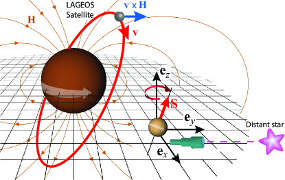
Figure 2: Star-fixed reference frame $S$: observers at rest in this frame form a rigid grid anchored to the asymptotic inertial frame where $g_{\alpha\beta}\to\eta_{\alpha\beta}$ (assumed fixed to the distant stars; experimentally, the spatial basis vectors $\mathbf{e}_{i}$ are set up by pointing telescopes to fixed stars). At infinity $S$ is inertial; at finite $r$, however, it is both accelerated and rotating. The associated Coriolis field $\mathbf{H}$ causes gyroscopes and satellite orbits to precess relative to $S$.

An example, depicted in Fig. 2, is the gravitational field of a spinning celestial body, such as Earth. In this case $\phi=-GM/r$, $\mathbf{G}=-GM\mathbf{r}/r^{3}$, and there is also a Coriolis field $\mathbf{H}$ created by the mass currents due to the Earth’s rotation. Given the similarity of Eq. (43) with the Maxwell-Ampère law, $\mathbf{A}$ and ${\bf H}$ can be obtained from the standard computation (e.g., Ref. Jackson, , Sec. 5.6) of the magnetic field created by a spinning charged body (replacing the vacuum magnetic permeability $\mu_{0}$ with $-16\pi G/c^{2}$ and the charge current with the mass current), leading to $\mathbf{A}=-2G\mathbf{J}\times\mathbf{r}/(c^{2}r^{3})$ and

$${\bf H}=\frac{2G}{c^{2}}\left(\frac{{\bf J}}{r^{3}}-\frac{3({\bf J}\cdot{\bf r}){\bf r}}{r^{5}}\right)$$ (51)

(cf., e.g., Eq. (6.1.25) of Ref. Gravitation and Inertia, ), where ${\bf J}$ is Earth’s angular momentum.

These fields are measured in the reference frame $S$ associated to the coordinate system of the metric (35). The frame $S$ is rigid and inertial at infinity (where the metric becomes flat, as both $\phi$ and $\mathbf{A}$ vanish); it is said to be fixed to the “distant stars.” However, at finite $r$ it is both an accelerated and rotating frame, as observers at rest in $S$ (fixed to the rigid grid in Fig. 2) are not freely falling: their acceleration is $\mathbf{a}=GM\mathbf{r}/r^{3}=-\mathbf{G}$, as is well known, and their vorticity is $\boldsymbol{\omega}=\mathbf{H}/2$. Note that $\boldsymbol{\omega}$ is an invariant, local measure of rotation. Just like in fluid dynamics, where at a given point the vorticity yields the angular velocity of rotation of the neighboring fluid particles (with respect to the “compass of inertia,” i.e. to inertial axes), $\boldsymbol{\omega}$ yields the angular velocity of rotation of the neighboring observers with respect to the compass of inertia. This so-called “compass of inertia”Gravitation and Inertia is a system of absolutely non-rotating axes, physically determined, both in classical mechanics and in general relativity, by the spin axes of local guiding gyroscopes. Hence, an immediate physical manifestation of the rotation of $S$ is the fact that gyroscopes are seen to “precess” relative to it. Such precession, known as the Lense-Thirring precession, was recently detected by the Gravity Probe B experiment.GravityProbeB This precession can be obtained by the same procedure of Sec. II, yielding Eq. (34) [now in terms of the Coriolis field (51)]. Equation (34) actually holds even in the exact theory, and not just in the weak field regime (cf., e.g., Eq. (63) of Ref. paperanalogies, ).

Another manifestation of the Coriolis field (51) that arises in $S$ is the deflection of test particles due to the Coriolis force $m\mathbf{v}\times\mathbf{H}$; it has been detected by measuring the orbital precession of the LAGEOS satellites,Ciufolini Lageos and there is an ongoing space mission (the LARES mission)LARES whose primary goal is to improve the accuracy of this measurement. The effect is again readily computed in the framework above: from Eq. (48) it follows that the variation of the orbital angular momentum ${\bf L}=m{\bf r}\times{\bf v}$ is given by

$$\frac{d{\bf L}}{dt}=m{\bf r}\times({\bf v}\times{\bf H})\$$ (52)

(since ${\bf r}\times{\bf G}={\bf 0}$).

We close this section with the following remarks. We have seen that $\mathbf{H}$ is a Coriolis field formally similar to the one of Newtonian mechanics (and as such, a field of fictitious forces). But it is purely relativistic, in the sense that it arises in a star fixed frame (where its Newtonian counterpart vanishes) due to the frame-dragging effect produced by mass currents. It is instructive to think about frame-dragging in terms of a Coriolis field, as it averts some common misconceptions about this effect in the literature (in particular those arising from the fluid dragging analogy proposed by some authors); for a detailed discussion of these problems we refer the reader to Ref. Rindler, .

IV Conclusion

In this work we discussed the Coriolis field in different settings; although its effects are familiar in some situations, there exist other, seemingly mysterious phenomena, that are simply effects of a Coriolis field.

We started with the example of an astronaut freely falling inside a rotating ship, whose motion from the point of view of the ship frame is puzzling until one realizes the role of the Coriolis field. We proceeded by showing that the Coriolis field satisfies the field equations of the so-called Newton-Cartan theory, a generalization of Newtonian theory that is covariant under changes of rigid (arbitrarily accelerated and rotating) frame. We presented simple solutions of this theory, including the Newtonian analogue of the Gödel universe, whose homogeneous rotation is easily understood in this framework.

Finally, we discussed the purely relativistic Coriolis field generated by mass currents. It is usually cast in the literature as a “gravitomagnetic field,” whose physical meaning—namely that it is just a Coriolis field, arising from the fact that the star fixed reference frame is in fact rotating close to mass currents—is often not transparent. The Lense-Thirring precession of the Gravity Probe B mission gyroscopes is seen to come from the same principle as the Newtonian precession of a gyrocompass relative to an Earth-fixed frame, and both are obtained by a computation analogous to that yielding the precession of a magnetic dipole in a magnetic field. The Lense-Thirring orbital precession of the LAGEOS/LARES satellites is also simply explained in terms of the Coriolis force, analogous to the Newtonian deflection of test particles in a rotating frame. Thinking in terms of a Coriolis field gives a correct, simple interpretation of the frame-dragging effect, avoiding the misconceptions about this effect that are all too common in the literature.

Appendix A Formulae for Sec. III

A.1 Linearized Christoffel Symbols

The Christoffel symbols are given, in terms of the metric tensor, as (e.g., Eq. (3.1) of Ref. Carroll, )

$$\Gamma_{\beta\gamma}^{\alpha}=\frac{1}{2}g^{\alpha\delta}(\partial_{\gamma}g_{\delta\beta}+\partial_{\beta}g_{\delta\gamma}-\partial_{\delta}g_{\beta\gamma})\ .$$ (53)

For the metric in Eq. (35), the linearized Christoffel symbols are obtained by neglecting all the terms that are not linear in the perturbations $\phi$ and $A_{i}$; they read

$$\Gamma_{00}^{0} =0\ ;\quad\Gamma_{00}^{i}=\frac{1}{c^{2}}\partial^{i}\phi=-\frac{1}{c^{2}}G^{i}=\Gamma_{i0}^{0}\ ;$$ (54)

$$\Gamma_{jk}^{0} =-\frac{1}{2c}(\partial_{j}A_{k}+\partial_{k}A_{j})\ ;\quad\Gamma_{0k}^{j}=\frac{1}{2c}(\partial_{k}A^{j}-\partial^{j}A_{k})\ ;$$ (55)

$$\Gamma_{kl}^{j} =\frac{1}{c^{2}}(\delta_{kl}\partial^{j}\phi-\delta^{j}_{l}\partial_{k}\phi-\delta^{j}_{k}\partial_{l}\phi)$$

$$=\frac{1}{c^{2}}(\delta^{j}_{l}G_{k}+\delta^{j}_{k}G_{l}-\delta_{kl}G^{j})\ ,$$ (56)

where we used the fact that, since $\phi$ and $A_{i}$ are time independent, all the time derivatives $\partial_{0}=(1/c)\partial/\partial t$ vanish. Note also that, to linear order, spatial indices are raised and lowered with the Kronecker delta, and so their vertical position is immaterial.

A.2 Linearized Ricci tensor

The Ricci tensor $R_{\beta\delta}$ is defined in terms of the Riemann curvature tensor $R_{\ \beta\gamma\delta}^{\alpha}$ as $R_{\beta\delta}\equiv R_{\ \beta\alpha\delta}^{\alpha}$. The Riemann tensor is given by, e.g., Eq. (3.113) of Ref. Carroll, ; to linear order $R_{\ \beta\gamma\delta}^{\alpha}=\partial_{\gamma}\Gamma_{\beta\delta}^{\alpha}-\partial_{\delta}\Gamma_{\beta\gamma}^{\alpha}$, and so

$$R_{\beta\delta}=\partial_{\alpha}\Gamma_{\beta\delta}^{\alpha}-\partial_{\delta}\Gamma_{\beta\alpha}^{\alpha}\ .$$ (57)

For the metric (35), the time-time component reads

$$R_{00}=\partial_{k}\Gamma_{00}^{k}=\frac{1}{c^{2}}\partial^{k}\partial_{k}\phi=-\frac{1}{c^{2}}\nabla\cdot\mathbf{G}\,,$$ (58)

while the time-space components $R_{0i}=R_{i0}$ are

$$R_{0i}=\partial_{j}\Gamma_{0i}^{j}=\frac{1}{2c}\partial^{j}\left(\partial_{i}A_{j}-\partial_{j}A_{i}\right)\,.$$ (59)

Noting that $H^{k}=(\nabla\times\textbf{A})^{k}=\epsilon^{kmn}\partial_{m}A_{n}$, it follows that $\epsilon_{ijk}H^{k}=\epsilon_{kij}\epsilon^{kmn}\partial_{m}A_{n}=\partial_{i}A_{j}-\partial_{j}A_{i}$, and therefore

$$R_{0i}=\frac{1}{2c}\epsilon_{ijk}\partial^{j}H^{k}=\frac{1}{2c}(\nabla\times\textbf{H})_{i}\ .$$ (60)

Lastly, the space-space components are

$$R_{ij} =\partial_{k}\Gamma_{ij}^{k}-\partial_{j}\Gamma_{ik}^{k}-\partial_{j}\Gamma_{i0}^{0}=-\frac{1}{c^{2}}(\nabla\cdot\mathbf{G})\delta_{ij}\ .$$ (61)

A.3 Linearized Einstein equations

For a non-relativistic source, $T^{00}=\rho c^{2}$, $T^{0i}\equiv cj^{i}=\rho cv_{{\rm matter}}^{i}$, $T^{ij}=\mathcal{O}(\rho v_{{\rm matter}}^{2})$; this means that

$$|T^{ij}|\sim|T^{00}|\frac{v_{{\rm matter}}^{2}}{c^{2}}\ll|T^{00}|\ ,$$ (62)

and therefore $T_{\ \gamma}^{\gamma}=T_{\ 0}^{0}+T_{\ i}^{i}\simeq T_{\ 0}^{0}=-\rho c^{2}$. The Einstein equations (41) then become, in this regime,

$$R_{\alpha\beta}=\frac{8\pi G}{c^{4}}\left(T_{\alpha\beta}^{\ }+\frac{1}{2}g_{\alpha\beta}^{\ }\rho c^{2}\right)\ .$$ (63)

To linear order (which implies neglecting also terms involving products of $\rho$ with the metric perturbations), the time-time component of Eq. (63) yields $R_{00}=4\pi G\rho/c^{2}$; equating this expression to Eq. (58) leads to Eq. (42). The time-space components yield

$$R_{0i}=\frac{8\pi G}{c^{3}}T_{0i}=-\frac{8\pi G}{c^{3}}j_{i}\,,$$ (64)

and equating this expression to Eq. (60) yields Eq. (43). As for the space-space components, using (62) we get $R_{ij}=4\pi G\rho\delta_{ij}/c^{2}$, and equating to Eq. (61) leads to Eq. (42) (the same as the time-time component).

A.4 Geodesic Equation

Starting from the geodesic equation (46), by repeated use of $d/d\tau=(dt/d\tau)d/dt$, one obtains

$$\frac{d}{d\tau}\left(\frac{dt}{d\tau}\frac{dr^{\alpha}}{dt}\right)+\left(\frac{dt}{d\tau}\right)^{2}\Gamma_{\beta\gamma}^{\alpha}\frac{dr^{\beta}}{dt}\frac{dr^{\gamma}}{dt}=0$$

$$\Leftrightarrow\frac{dr^{\alpha}}{dt}\frac{d^{2}t}{d\tau^{2}}+\left(\frac{dt}{d\tau}\right)^{2}\frac{d^{2}r^{\alpha}}{dt^{2}}+\left(\frac{dt}{d\tau}\right)^{2}\Gamma_{\beta\gamma}^{\alpha}\frac{dr^{\beta}}{dt}\frac{dr^{\gamma}}{dt}=0\ .$$ (65)

Now, since $t=r^{0}/c$, using Eq. (46), we have

$$\frac{d^{2}t}{d\tau^{2}} =\frac{1}{c}\frac{d^{2}r^{0}}{d\tau^{2}}=-\frac{1}{c}\Gamma_{\beta\gamma}^{0}\frac{dr^{\beta}}{d\tau}\frac{dr^{\gamma}}{d\tau}$$

$$=-\frac{1}{c}\left(\frac{dt}{d\tau}\right)^{2}\Gamma_{\beta\gamma}^{0}\frac{dr^{\beta}}{dt}\frac{dr^{\gamma}}{dt}\,.$$ (66)

Substituting this expression back into Eq. (65) leads to Eq. (47).

References

- (1) Actually, in a gratifying acknowledgment of angular momentum conservation, they use two counter-rotating spinning wheels.
- (2) <http://www.badastronomy.com/bad/movies/redplanet2.html>.
- (3) A. Einstein, The Meaning of Relativity, Ed. (Princeton University Press, Princeton, 2014).
- (4) These terms are minus the acceleration of the origin of the frame , the centrifugal force per unit mass , and the so-called Euler force per unit mass .
- (5) W. Cox, Vector Calculus (Butterworth-Heinemann, 1998), p. 171.
- (6) The Newton-Cartan theory is more often presented in terms of the so-called Cartan connection. Here we show this theory as written on a rigid frame, with the connection coefficients reinterpreted as the fields and . See L. Godinho and J. Natário, An Introduction to Riemannian Geometry: With Applications to Mechanics and Relativity (Springer, New York, 2014).
- (7) F. Rohrlich, “The logic of reduction: the case of gravitation,” Found. Phys. 19, 1151–1170 (1989).
- (8) G. Dautcourt, “On the Newtonian limit of general relativity,” Acta Phys. Pol. B21, 755–765 (1990).
- (9) J. Ehlers, The Newtonian limit of general relativity, in G. Ferrarese, ed., Classical Mechanics and Relativity: Relationship and Consistency (Bibliopolis, Napoli, 1991).
- (10) J. Ehlers, “Examples of Newtonian limits of relativistic spacetimes,” Class. Quant. Grav. 14, A119–A126 (1997).
- (11) K. Gödel, “An example of a new type of cosmological solution of Einstein’s field equations of gravitation,” Rev. Mod. Phys. 21, 447–450 (1949).
- (12) K. Gödel, Lecture on rotating universes, in Feferman et al., eds., Kurt Gödel Collected Works, Vol. III (Oxford University Press, Oxford, 1995).
- (13) I. Ozsváth and E. Schucking, “Approaches to Gödel’s rotating universe,” Class. Quant. Grav. 18, 2243–2252 (2001).
- (14) I. Ozsváth and E. Schucking, “Gödel’s trip,” Am. J. Phys. 71, 801–805 (2003).
- (15) This is best seen by considering the inverse change of frame, to which Eqs. (12) and (13) apply.
- (16) E. Milne, “A Newtonian expanding universe,” Quart. J. Math. 5, 64–72 (1934).
- (17) W. McCrea and E. Milne, “Newtonian universes and the curvature of space,” Quart. J. Math. 5, 73–80 (1934).
- (18) J. Jackson, Classical Electrodynamics, Ed. (John Wiley & Sons, New York, 1998).
- (19) This is not really a potential energy, since the magnetic field cannot do work. See, e.g., R. Young, “Nonrelativistic rotating charged sphere as a model for particle spin,” Am. J. Phys. 44, 581–588 (1976) and C. Coombes, “Work done on charged particles in magnetic fields,” Am. J. Phys. 47, 915–916 (1979).
- (20) M. Levi, Classical Mechanics With Calculus of Variations and Optimal Control: An Intuitive Introduction (American Mathematical Society, 2014), Sec. 3.11.
- (21) There is a huge literature about the analogies between electromagnetism and gravity in different regimes; see Refs. paperanalogies, ; GEM User Manual, and references therein.
- (22) L. F. Costa and J. Natário, “Gravito-electromagnetic analogies,” Gen. Rel. Grav. 46, 1792-1–57 (2014).
- (23) R. Jantzen, P. Carini and D. Bini, GEM: the User Manual (2004). <http://www34.homepage.villanova.edu/robert.jantzen/gem/gemgrqc.pdf>
- (24) H. Stephani, Relativity: An Introduction to Special and General Relativity, Ed. (Cambridge Univ. Press, 2004), Sec. 27.
- (25) E. Harris, “Analogy between general relativity and electromagnetism for slowly moving particles in weak gravitational fields,” Am. J. Phys. 59, 421–425 (1991).
- (26) I. Ciufolini and J. Wheeler, Gravitation and Inertia (Princeton University, Princeton, NJ, 1995).
- (27) S. Carroll, Spacetime and Geometry: An Introduction to General Relativity (Addison Wesley, San Francisco, 2004), Ch. 7.
- (28) The exact version of Eqs. (42)–(45) is obtained from Eqs. (90)–(91) and (93)–(94) of Ref. paperanalogies, taking the case of rigid frames ( therein) and a dust source, and restoring the and factors ( in the unit system of Ref. paperanalogies, ). They read , , , , where . These equations yield Eqs. (21) exactly when .
- (29) L. Landau and E. Lifshitz, The Classical Theory of Fields (Butterworth-Heinemann, Oxford, 1997).
- (30) C. Everitt et al., “Gravity Probe B: Final results of a space experiment to test general relativity,” Phys. Rev. Lett. 106, 221101-1–5 (2011). The GP-B mission measured not only the Lense-Thirring precession due to the rotation of the Earth, but also the (much larger) geodetic effect, arising from the fact that the gyroscope was in orbit (so in the gyroscope’s frame the Earth had both rotational and translational motion).
- (31) I. Ciufolini and E. Pavlis, “A confirmation of the general relativistic prediction of the Lense-Thirring effect,” Nature 431, 958–960 (2004).
- (32) I. Ciufolini et al., “Towards a one percent measurement of frame dragging by spin with satellite laser ranging to LAGEOS, LAGEOS 2 and LARES and GRACE gravity models,” Space Sci. Rev. 148, 71–104 (2009); <http://www.lares-mission.com/>
- (33) W. Rindler, “The case against space dragging,” Phys. Lett. A 223, 25–29 (1997).