Two-dimensional inflow-wind solution of black hole accretion with an evenly symmetric magnetic field

Abstract

We solve the two-dimensional magnetohydrodynamic (MHD) equations of black hole accretion with the presence of magnetic field. The field includes a turbulent component, whose role is represented by the viscosity, and a large-scale ordered component. The latter is further assumed to be evenly symmetric with the equatorial plane. The equations are solved in the $r-\theta$ plane of a spherical coordinate by assuming time-steady and radially self-similar. An inflow-wind solution is found. Around the equatorial plane, the gas is inflowing; while above and below the equatorial plane at a certain critical $\theta$ angle, $\theta\sim 47^{\circ}$, the inflow changes its direction of radial motion and becomes wind. The driving forces are analyzed and found to be the centrifugal force and the gradient of gas and magnetic pressure. The properties of wind are also calculated. The specific angular momentum of wind is found to be significantly larger than that of inflow, thus wind can transfer angular momentum outward. These analytical results are compared to those obtained by the trajectory analysis based on MHD numerical simulation data and good agreements are found.

1 Introduction

Black hole accretion models can be divided into hot and cold types according to the temperature of the accretion flow. Since the pioneer work of Narayan & Yi (1994) (see also Ichimaru 1977; Rees et al. 1982), intensive studies have been performed on black hole hot accretion flows. It is now known that hot accretion flow is very common in the universe, ranging from low-luminosity active galactic nuclei (LLAGNs), which is the majority of nearby galaxies, to the quiescent and hard states of black hole X-ray binaries. Yuan & Narayan (2014) have recently reviewed our current understanding of hot accretion flows, including its one-dimensional and multi-dimensional dynamics, jet formation, radiation, and various astrophysical applications.

One of the most interesting topics in recent years in this field is wind (also often called outflow). Wind is not only a fundamental aspect of accretion flow, but also plays an important role in AGN feedback, since wind can suppress the star formation and black hole growth effectively (e.g., Ostriker et al. 2010). The study of wind was initiated by the hydrodynamical and MHD numerical simulations of accretion flows (Stone, Pringle & Begelman 1999; Igumenshchev & Abramowicz 1999, 2000; Stone & Pringle 2001). These simulations found that in contrast to our original picture, the mass accretion rate decreases with decreasing radius (see review in Yuan et al. 2012b). To explain such an astonishing result, two models have been proposed, namely convection-dominated accretion flow (CDAF; Narayan et al. 2000; Quataert & Gruzinov 2000) and adiabatic inflow-outflow solution (ADIOS; Blandford & Begelman 1999). By comparing the properties of inflow and outflow and studying the convective stability of MHD accretion flow, Yuan et al. (2012a; see also Li, Ostriker & Sunyaev 2013) show that strong wind must exist and it is the wind rather than convection that results in the inward decrease of accretion rate. Most recently, based on MHD simulation data, Yuan et al. (2015) have convincingly show the existence of strong wind by obtaining the trajectory of the virtual test particles based on 3D GRMHD simulation data of black hole accretion. Moreover, the driving forces of wind have also been analyzed and the detailed properties of winds have been calculated, such as the mass flux, angular distribution, terminal velocity, and fluxes of energy and momentum. The theoretical study on the existence of strong wind has been confirmed by the detection of emission lines from the accretion flow around the supermassive black hole in the Galactic center, Sgr A* (Wang et al. 2013). As an application of the accretion wind theory, more recently, the formation of the Fermi bubbles detected by the Fermi telescope in the Galaxy has been successfully explained by the interaction of wind launched from the accretion flow around Sgr A* and the interstellar medium (Mou et al. 2014; 2015). Compared to other theoretical models of the Fermi bubbles, this “accretion-wind” model has two advantages. One is that the parameters of wind adopted in the model are taken from the MHD simulation of accretion flow. The second one is that the model can explain the new observational results obtained by Suzaku and Chandra which are in conflict with the predictions of other models.

Almost all of the above-mentioned theoretical works on wind are numerical. Compared to numerical simulations, analytical study has its advantage of more clearly revealing some underlying physics. In this paper, using analytical method, we solve the axisymmetric steady solution of hot accretion flow with the presence of magnetic field. Self-similar assumption is adopted as in many previous works. Special attention is paid to whether the winds exist in the solution and what are their driving mechanisms if they exist. The aim is to compare with the numerical results presented in Yuan et al. (2015) thus to improve our understanding of numerical studies.

There have been many analytical works based on the self-similar assumption. In the one-dimensional works, the existence of wind is often an assumption (e.g. Blandford & Begelman 1999; Akizuki & Fukue 2006; Abbassi et al. 2008; Zhang & Dai 2008; Bu et al. 2009). Winds have been found in some two-dimensional solutions (e.g. Xu & Chen 1997; Blandford & Begelman 2004; Xue & Wang 2005; Tanaka & Menou 2006; Jiao & Wu 2011; Mosallanezhad et al. 2014; Gu 2015; Samadi & Abbassi 2016 ) but not all (e.g., Narayan & Yi 1995 and references therein). In all these works magnetic field is not included. It is well known that magnetic field must be present and even plays an important role in the dynamics of accretion flow, such as the angular momentum transfer by MRI (Balbus & Hawley 1998), the convective stability of accretion flow, which is related with the wind production (Yuan et al. 2012a; Narayan et al. 2012), and the driving mechanism of winds (Yuan et al. 2015). So it is useful to solve the accretion solutions by including magnetic field. This is the aim of the present paper.

The organization of the paper is as follows. In §2, the basic MHD equations and assumptions are given. The numerical solutions of the equations are described in §3. The results are summarized in §4.

2 Basic MHD equations

The basic MHD equations describing accretion flows read:

$$\frac{d\rho}{dt}+\rho\mathbf{\nabla}\cdot\mathbf{v}=0,$$ (1)

$$\rho\frac{d\mathbf{v}}{dt}=-\rho\mathbf{\nabla}\Psi-\mathbf{\nabla}p+\nabla\cdot\mathbf{T}+\frac{1}{c}\left(\mathbf{J}\times\mathbf{B}\right),$$ (2)

$$\rho\frac{de}{dt}-\frac{p}{\rho}\frac{d\rho}{dt}=fQ^{+},$$ (3)

$$\frac{\partial\mathbf{B}}{\partial t}=\mathbf{\nabla}\times\left(\mathbf{v}\times\mathbf{B}-\frac{4\pi}{c}\eta\mathbf{J}\right),$$ (4)

$$\mathbf{\nabla}\cdot\mathbf{B}=0.$$ (5)

In the above equations, $\rho$, $\mathbf{v}$, $p$, $e$, $\mathbf{T}$, $\mathbf{B}$ and $\eta$ denote the density, velocity, gas pressure, gas internal energy, viscous stress tensor, magnetic field, and magnetic diffusivity, respectively. We adopt an equation of state of ideal gas, $p=(\gamma-1)\rho e$, where $\gamma$ is the specific heat ratio. A spherical coordinate ($r$, $\theta$, $\phi$) is adopted in the present work. $\Psi(=-GM/r)$ is the Newtonian gravitational potential, where $M$ is the mass of the central black hole, $G$ is the gravitational constant. $\mathbf{J}\equiv c/4\pi(\mathbf{\nabla}\times\mathbf{B})$ is the electric current. We must include this dissipation term in eq. (4), because otherwise we can’t obtain the steady solution due to the accumulation of magnetic flux in the accretion. $Q^{+}$ is the heating rate. $f$ is the advection factor describing the fraction of the heating energy which is stored in the gas and advected into the black hole. In this paper, we set $f=1$. The heating rate $Q^{+}$ can be decomposed into two components,

$$Q^{+}=Q_{vis}+Q_{res},$$ (6)

with $Q_{vis}$ and $Q_{res}$ denoting the viscous heating and the magnetic field dissipation heating, respectively. Following Stone et al. (1999), we assume that the only non-zero component of the viscous tensor $\mathbf{T}$ is the azimuthal component,

$$T_{r\phi}=\rho\nu r\frac{\partial(v_{\phi}/r)}{\partial r},$$ (7)

where $\nu$ is the kinematic viscosity. The viscous heating and the magnetic field dissipation heating can be described as,

$$Q_{vis}=T_{r\phi}r\frac{\partial}{\partial r}\left(\frac{v_{\phi}}{r}\right),$$ (8)

$$Q_{res}=\frac{4\pi}{c^{2}}\eta\mathbf{J}^{2}.$$ (9)

We adopt the usual $\alpha$ description of viscosity $\nu=\alpha p/(\rho\Omega_{K})$, where $\Omega_{K}=(GM/r^{3})^{1/2}$ is the Keplerian angular velocity. In order to satisfy the radial self-similar condition we assume the magnetic diffusivity $\eta=\eta_{0}p/(\rho\Omega_{K})$.

Following the suggestion from numerical MHD simulations, we decompose the magnetic field into a large-scale component and a turbulent component. Both of them can transfer the angular momentum and can be dissipated and produce heat. The magnetic field $\mathbf{B}$ in equations (2), (4) and (5) corresponds to the former. We describe the effects of the turbulent component of the magnetic field in transferring the angular momentum and in dissipating the energy through the usual $\alpha$ description. Specifically, the viscous force $\nabla\cdot\mathbf{T}$ in equation (2) represents angular momentum transfer by the turbulent magnetic field; the viscous heating rate $Q_{vis}$ in equation (6) is correspondingly associated with the turbulent component of the magnetic field.

We assume that the large-scale magnetic field is evenly symmetric about the equatorial plane (see Figure 1 for the poloidal configuration of the magnetic field). This kind of symmetry is widely adopted in the studies of accretion disks (e.g. Blandford & Payne 1982; Lovelace et al. 1994; Cao 2011; Li & Begelman 2014). Thus we have,

$$B_{r}(r,\theta)=-B_{r}(r,\pi-\theta),$$ (10)

$$B_{\theta}(r,\theta)=+B_{\theta}(r,\pi-\theta),$$ (11)

$$B_{\phi}(r,\theta)=-B_{\phi}(r,\pi-\theta),$$ (12)

A toroidal component of the magnetic field is generated due to the shear of the accretion flow. Therefore the radial and the toroidal components of the magnetic field should have opposite sign. In this paper, we only focus on the region above the equatorial plane, we set the radial component of themagnetic field to be positive ($B_{r}>0$). Therefore, the toroidal component of the magnetic field generated by shear is negative ($B_{\phi}<0$).

We solve for the steady state, axisymmetric ($\partial/\partial t=\partial/\partial\phi=0$) solutions of eqs. 1-5. The continuity equation can be rewritten as:

$$\frac{1}{r^{2}}\frac{\partial}{\partial r}\left(r^{2}\rho v_{r}\right)+\frac{1}{r\sin\theta}\frac{\partial}{\partial\theta}\left(\sin\theta\rho v_{\theta}\right)=0,$$ (13)

The momentum equation (2) reads:

$$\rho\left[v_{r}\frac{\partial v_{r}}{\partial r}+\frac{v_{\theta}}{r}\left(\frac{\partial v_{r}}{\partial\theta}-v_{\theta}\right)-\frac{v_{\phi}^{2}}{r}\right]=-\rho\frac{GM_{*}}{r^{2}}-\frac{\partial p}{\partial r}\\ +\frac{1}{4\pi}\left(J_{\theta}B_{\phi}-J_{\phi}B_{\theta}\right),$$ (14)

$$\rho\left[v_{r}\frac{\partial v_{\theta}}{\partial r}+\frac{v_{\theta}}{r}\left(\frac{\partial v_{\theta}}{\partial\theta}+v_{r}\right)-\frac{v_{\phi}^{2}}{r}\cot\theta\right]=-\frac{1}{r}\frac{\partial p}{\partial\theta}\\ +\frac{1}{4\pi}\left(J_{\phi}B_{r}-J_{r}B_{\phi}\right),$$ (15)

$$\rho\left[v_{r}\frac{\partial v_{\phi}}{\partial r}+\frac{v_{\theta}}{r}\frac{\partial v_{\phi}}{\partial\theta}+\frac{v_{\phi}}{r}\left(v_{r}+v_{\theta}\cot\theta\right)\right]=\frac{1}{r^{3}}\frac{\partial}{\partial r}\left(r^{3}T_{r\phi}\right)\\ +\frac{1}{4\pi}\left(J_{r}B_{\theta}-J_{\theta}B_{r}\right),$$ (16)

where the current ($\mathbf{J}$) reads:

$$J_{r}=\frac{1}{r\sin\theta}\frac{\partial}{\partial\theta}\left(B_{\phi}\sin\theta\right),$$ (17)

$$J_{\theta}=-\frac{1}{r}\frac{\partial}{\partial r}\left(rB_{\phi}\right),$$ (18)

$$J_{\phi}=\frac{1}{r}\left[\frac{\partial}{\partial r}\left(rB_{\theta}\right)-\frac{\partial B_{r}}{\partial\theta}\right].$$ (19)

The equation of energy is expressed as:

$$\rho\left(v_{r}\frac{\partial e}{\partial r}+\frac{v_{\theta}}{r}\frac{\partial e}{\partial\theta}\right)-\frac{p}{\rho}\left(v_{r}\frac{\partial\rho}{\partial r}+\frac{v_{\theta}}{r}\frac{\partial\rho}{\partial\theta}\right)=\\ f\left(T_{r\phi}r\frac{\partial}{\partial r}\left(\frac{v_{\phi}}{r}\right)+\frac{\eta}{4\pi}\left(J_{r}^{2}+J_{\theta}^{2}+J_{\phi}^{2}\right)\right).$$ (20)

The three components of induction equation (4) can be expressed as:

$$\frac{\partial B_{r}}{\partial t}=\frac{\partial}{\partial\theta}\left[r\sin\theta\left(v_{r}B_{\theta}-v_{\theta}B_{r}-\eta J_{\phi}\right)\right],$$ (21)

$$\frac{\partial B_{\theta}}{\partial t}=\frac{\partial}{\partial r}\left[r\sin\theta\left(v_{r}B_{\theta}-v_{\theta}B_{r}-\eta J_{\phi}\right)\right],$$ (22)

$$\frac{\partial B_{\phi}}{\partial t}=\frac{\partial}{\partial r}\left(rv_{\phi}B_{r}-rv_{r}B_{\phi}\right)+\frac{\partial}{\partial\theta}\left(v_{\phi}B_{\theta}-v_{\theta}B_{\phi}\right)+\frac{\partial}{\partial\theta}\left(\eta J_{r}\right)\\ -\frac{\partial}{\partial r}\left(r\eta J_{\theta}\right).$$ (23)

For a steady state, the right hand side of equations (21), (22) and (23) has to be equal to zero. So we have $r\sin\theta\left(v_{r}B_{\theta}-v_{\theta}B_{r}-\eta J_{\phi}\right)=0$ or a constant. In this paper, we assume it is equal to zero:

$$r\sin\theta\left(v_{r}B_{\theta}-v_{\theta}B_{r}-\eta J_{\phi}\right)=0.$$ (24)

Finally, the divergence-free equation (5) can be written as,

$$\frac{1}{r^{2}}\frac{\partial}{\partial r}\left(r^{2}B_{r}\right)+\frac{1}{r\sin\theta}\frac{\partial}{\partial\theta}\left(\sin\theta B_{\theta}\right)=0.$$ (25)

Similar to previous works (e.g., Narayan & Yi 1995; Xue & Wang 2005; Jiao & Wu 2011), we seek the radially self-similar solutions in the following forms:

$$\rho(r,\theta)=\rho(\theta)r^{-n},$$ (26)

$$v_{r}(r,\theta)=\sqrt{\frac{GM}{r}}v_{r}(\theta)=r\Omega_{K}(r)v_{r}(\theta),$$ (27)

$$v_{\theta}(r,\theta)=r\Omega_{K}(r)v_{\theta}(\theta),$$ (28)

$$v_{\phi}(r,\theta)=r\Omega_{K}(r)v_{\phi}(\theta),$$ (29)

$$p(r,\theta)=p(\theta)GMr^{-n-1},$$ (30)

$$B_{r}(r,\theta)=b_{r}(\theta)\sqrt{GM}r^{-(n/2)-(1/2)},$$ (31)

$$B_{\theta}(r,\theta)=b_{\theta}(\theta)\sqrt{GM}r^{-(n/2)-(1/2)},$$ (32)

$$B_{\phi}(r,\theta)=b_{\phi}(\theta)\sqrt{GM}r^{-(n/2)-(1/2)}.$$ (33)

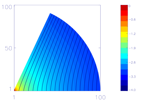
Figure 1: Solid lines represent the magnetic field line. Colors show the logarithm angular velocity ($v_{\phi}/r$). It is clear that moving along the magnetic field lines starting from the equatorial plane, the angular velocity decreases. Therefore, if we assume that $B_{r}$ above the equatorial plane is positive, shear of the flow will produce a negative $B_{\phi}$.

Using the above self-similar assumptions, equations (13)-(16), (20), (23)-(25) can be written as,

$$v_{\theta}\frac{d\ln\rho}{d\theta}+\left(\frac{3}{2}-n\right)v_{r}+v_{\theta}\cot\theta+\frac{dv_{\theta}}{d\theta}=0,$$ (34)

$$\rho\left[-\frac{1}{2}v^{2}_{r}+v_{\theta}\frac{dv_{r}}{d\theta}-v^{2}_{\theta}-v^{2}_{\phi}\right]=-\rho+(n+1)p\\ +\frac{1}{4\pi}\left(j_{\theta}b_{\phi}-j_{\phi}b_{\theta}\right),$$ (35)

$$\rho\left[\frac{1}{2}v_{r}v_{\theta}+v_{\theta}\frac{dv_{\theta}}{d\theta}-v_{\phi}^{2}\cot\theta\right]=-\frac{dp}{d\theta}\\ +\frac{1}{4\pi}\left(j_{\phi}b_{r}-j_{r}b_{\phi}\right),$$ (36)

$$\rho\left[\frac{1}{2}v_{r}v_{\phi}+v_{\theta}\frac{dv_{\phi}}{d\theta}+v_{\theta}v_{\phi}\cot\theta\right]=\frac{3}{2}\alpha(n-2)pv_{\phi}\\ +\frac{1}{4\pi}\left(j_{r}b_{\theta}-j_{\theta}b_{r}\right),$$ (37)

$$(n\gamma-n-1)v_{r}p+v_{\theta}\frac{dp}{d\theta}-\gamma pv_{\theta}\frac{d\ln\rho}{d\theta}=\\ f\left(\gamma-1\right)\left(\frac{9}{4}\alpha pv_{\phi}^{2}+\frac{\eta}{4\pi}\left(j_{r}^{2}+j_{\theta}^{2}+j_{\phi}^{2}\right)\right),$$ (38)

$$\frac{n}{2}\left(v_{r}b_{\phi}-v_{\phi}b_{r}+\eta j_{\theta}\right)+v_{\phi}\frac{db_{\theta}}{d\theta}+b_{\theta}\frac{dv_{\phi}}{d\theta}-v_{\theta}\frac{db_{\phi}}{d\theta}-b_{\phi}\frac{dv_{\theta}}{d\theta}\\ +\eta\frac{dj_{r}}{d\theta}+j_{r}\frac{d\eta}{d\theta}=0,$$ (39)

$$\frac{db_{\theta}}{d\theta}-\frac{1}{2}(n-3)b_{r}+b_{\theta}\cot\theta=0.$$ (40)

where

$$\eta=\eta_{0}\frac{p}{\rho},$$ (41)

$$j_{r}=\frac{db_{\phi}}{d\theta}+b_{\phi}\cot\theta,$$ (42)

$$j_{\theta}=\frac{1}{2}(n-1)b_{\phi},$$ (43)

$$j_{\phi}=\frac{1}{\eta}\left(v_{r}b_{\theta}-v_{\theta}b_{r}\right).$$ (44)

Equations (34)-(40) are differential equations for eight variables: $v_{r}(\theta)$, $v_{\theta}(\theta)$, $v_{\phi}(\theta)$, $\rho(\theta)$, $p(\theta)$, $b_{r}(\theta)$, $b_{\theta}(\theta)$ and $b_{\phi}(\theta)$. In this paper, we assume the accretion flow is evenly symmetric about the equatorial plane, then $\rho(\theta)=\rho(\pi-\theta)$, $p(\theta)=p(\pi-\theta)$, $v_{r}(\theta)=v_{r}(\pi-\theta)$, $v_{\phi}(\theta)=v_{\phi}(\pi-\theta)$ and $v_{\theta}(\theta)=-v_{\theta}(\pi-\theta)$. At the equatorial plane, we have by symmetry:

$$\theta=\frac{\pi}{2}:b_{r}=v_{\theta}=\frac{dv_{r}}{d\theta}=\frac{dv_{\phi}}{d\theta}=\frac{d\rho}{d\theta}=\frac{dp}{d\theta}=\frac{db_{\theta}}{d\theta}=\frac{db_{\phi}}{d\theta}=0.$$ (45)

We set the density at the equatorial plane $\rho(\pi/2)=1$. Under the above boundary conditions, equations (34)-(40) can be simplified into the following equations,

$$\frac{dv_{\theta}}{d\theta}=\big{(}n-\frac{3}{2}\big{)}v_{r},$$ (46)

$$\frac{1}{2}v_{r}^{2}+v_{\phi}^{2}+\left(n+1\right)p+\frac{1}{4\pi}\left(\frac{1}{2}\left(n-1\right)b_{\phi}^{2}+\frac{v_{r}b_{\theta}^{2}}{\eta_{0}p}\right)=0,$$ (47)

$$v_{r}=3\alpha\left(n-2\right)p,$$ (48)

$$\left(n\gamma-n-1\right)v_{r}=f\left(\gamma-1\right)\times\\ \left[\frac{9}{4}\alpha v_{\phi}^{2}+\frac{\eta_{0}}{4\pi}\left(\left(\frac{1}{2}\left(n-1\right)b_{\phi}\right)^{2}+\left(\frac{v_{r}b_{\theta}}{\eta_{0}p}\right)^{2}\right)\right].$$ (49)

At the equatorial plane, we set the ratio of the magnetic pressure to the gas pressure as,

$$\beta_{\theta 0}=\frac{b^{2}_{\theta}}{8\pi p_{g}}\underset{\pi/2}{\bigg{|}},$$ (50)

$$\beta_{\phi 0}=\frac{b^{2}_{\phi}}{8\pi p_{g}}\underset{\pi/2}{\bigg{|}}.$$ (51)

In principle, to solve eqs. (34)-(40), in addition to the boundary condition at $\theta=90^{\circ}$, we should also supply the boundary condition at the rotation axis, i.e., $\theta=0^{\circ}$. Mathematically, this is a two-point boundary problem and it will assure that we have a well-behaved solution in the whole $r-\theta$ space. We have tried to obtain such solutions but failed. Therefore, we only require the solution satisfying the boundary condition at $\theta=90^{\circ}$. As we will explain in the next section, we think the solution obtained in this way should still be physically meaningful.

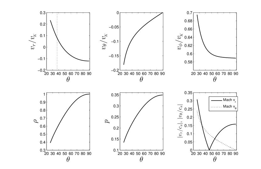
Figure 2: Angular profile of a variety of variables. The up-left plot shows that the radial velocity changes its sign at $\theta\sim 47^{\circ}$.

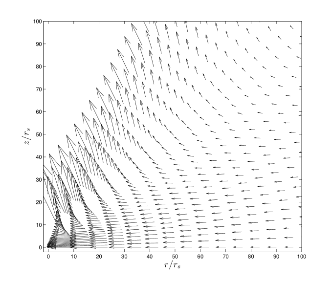
Figure 3: Stream lines of the accretion flow, showing the inflow-wind structure. The length of arrows indicates the absolute value of $\vec{v}_{r}+\vec{v}_{\theta}$.

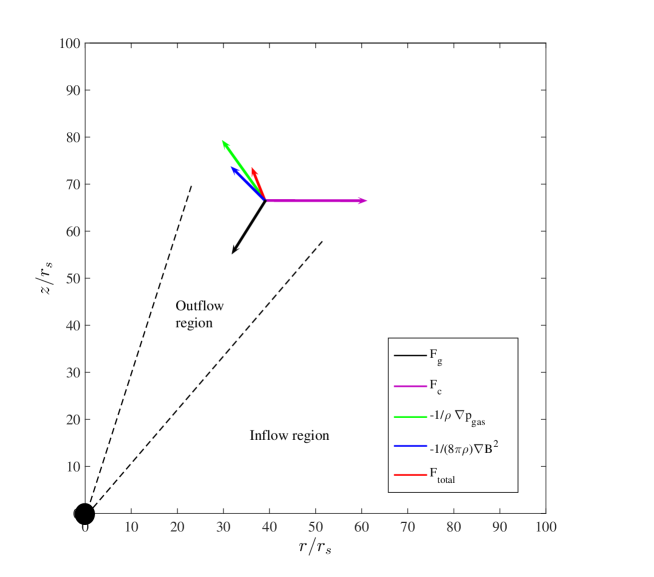
Figure 4: The force analysis at the wind region to show the driving mechanism of wind. The length of the arrows schematically denotes the magnitude of the forces while the direction for the direction of forces. $F_{g}$: graviational force; $F_{c}$: centrifugal force; $F_{\rm total}$: the total force.

3 Results

We solve the above equations (34)-(40) numerically. We integrate these equations from the equatorial plane ($\theta=90^{\circ}$) towards the rotational axis ($\theta=0^{\circ}$). We adopt the values of $\beta_{\theta 0}$ and $\beta_{\phi 0}$ with reference to the numerical simulation data of Yuan et al. (2012a), but our results are not sensitive to the exact values. As we have explained before, the toroidal component of the magnetic field, which is produced by shear, should be negative. We do find that the toroidal component is negative at the beginning of integration. But at a certain critical value of $\theta$, denoted as $\theta_{B}$, we find that it begins to change its sign. At the region of $\theta<\theta_{B}$, the toroidal component of the magnetic field becomes positive thus the solution is no longer physical so we stop our integration at $\theta_{B}$. We think our solution in the region of $\theta_{B}<\theta<90^{\circ}$ is still physical. This is because, on the one hand, the solution satisfies the equations and the boundary conditions at $\theta=90^{\circ}$. On the other hand, the values of all physical quantities of the accretion flow at $\theta=\theta_{B}$ are physical. Therefore, we can reasonably treat these values as boundary conditions at $\theta_{B}$. In fact, as we will describe below, the main properties of the solutions we obtain in this way are in good agreement with those obtained in Yuan et al. (2015) from numerical simulations.

From the bottom-right plot of Figure 2, it seems that there is a sonic point for $v_{\theta}/c_{s}$ and the integration stops when the sonic point is approached because of the singularity there. This is not true. This is because, the value of $v_{\theta}$ must be equal to zero at the pole because of the axisymmetric boundary condition there. Therefore, $v_{\theta}/c_{s}$ should not pass through a sonic point. We note that Jiao & Wu (2011) obtained a similar result with us, i.e., their solution also has to stop at a certain $\theta$ angle. An interesting explanation for such a “truncation” is given in their work.

3.1 Overall inflow-wind structure of the solutions

Figure 1 shows the poloidal magnetic field configuration. We emphasize that while the even symmetry of the field is our assumption, the strength of the field is obtained by solving equations (34)-(40). Above the equatorial plane, the radial component of the magnetic field is positive (pointing to large radii). So the toroidal component of the magnetic field, which is produced by shear, is negative. We find that such kind of magnetic field configuration is similar to the time-averaged field configuration in MHD numerical simulation in Yuan et al. (2012a) and Yuan et al. (2015).

Figure 2 presents the angular profiles of four quantities. The parameters we adopt are $\alpha=\eta_{0}=0.1,\gamma=5/3,\beta_{\theta 0}=2\times 10^{-4},\beta_{\phi 0}=2\times 10^{-3},n=0.85$ and $f=1$. From the equatorial plane to the rotation axis, the density and pressure decrease, while $v_{r}$ and $v_{\phi}$ increase. This is consistent with that in Jiao & Wu (2011). The value of $v_{\theta}$ is negative and its absolute value increases towards the pole. The Mach number $v_{\theta}/c_{s}$ increases towards the pole, this is also consistent with that found in Jiao & Wu (2011). However, we note that beyond $\theta_{B}$, $v_{\theta}$ have to decrease towards the pole and eventually become zero at pole due to the boundary condition there.

In the region of $47^{\circ}<\theta<90^{\circ}$, the radial velocity is negative. This is the inflow region. At the region of $\theta<47^{\circ}$, the radial velocity becomes positive, i.e., wind is evident. Figure 3 shows the steam line of the flow. This result is fully consistent with the results obtained in Yuan et al. (2015; see also Narayan et al. 2012; Sadowski et al. 2013). In those works, they also found that inflow is present around the equatorial plane of the accretion flow while wind is present in the polar region. The boundary between inflow and wind obtained in the present paper is even quantitatively similar to that obtained in Yuan et al. (2015). In both cases the boundary is located at about $\theta\sim 50^{\circ}-60^{\circ}$.

3.2 Angular momentum transfer by wind

The up-right panel of Figure 2 shows the rotation velocity of the accretion flow. We find that it significantly increases from the equatorial plane to the rotation axis, which suggests that the specific angular momentum of wind may be larger than that of inflow. To examine this point in more detail, we have calculated the mass flux-weighted specific angular momentum of both the wind and inflow (see Eqs. 8 & 9 in Yuan et al. (2012a) for the details of calculation). In unit of the Keplerian angular momentum $l_{K}$, the mass-flux weighted angular momentum of wind and inflow is found to be

$$l_{\rm wind}=0.67l_{K},~{}~{}~{}~{}l_{\rm inflow}=0.59l_{K},$$ (52)

respectively. This result means that wind can transfer the angular momentum of the accretion flow. This result is again consistent with the numerical simulation result presented in Yuan et al. (2012a).

To compare the efficiency of angular momentum transfer by outflow and by viscosity, we calculate the angular momentum flux transported by outflow and viscosity as follows

$${F}_{L\rm out}=2\pi r^{2}\int_{\theta_{B}}^{\pi/2}\rho\max(v_{r},0)(rv_{\phi})\sin\theta d\theta,$$ (53)

$${F}_{L\rm vis}=2\pi r^{2}\int_{\theta_{B}}^{\pi/2}rT_{r\phi}\sin\theta d\theta.$$ (54)

We find

$$\frac{F_{L\rm out}}{F_{L\rm vis}}=0.26.$$ (55)

This means outflows do play an important role in transferring angular momentum.

3.3 Poloidal speed of wind

We have also calculated the mass flux-weighted poloidal speed $v_{p}(\equiv\sqrt{v_{r}^{2}+v_{\theta}^{2}}$) of winds when they are just launched. The result is

$$v_{p}(r)=0.18\ v_{K}(r),$$ (56)

where $v_{K}$ is the Keplerian velocity. This is consistent with that obtained in Yuan et al. (2015), where they found that $v_{p}\approx 0.2v_{K}(r)$.

3.4 Bernoulli parameter and terminal velocity of wind

The Bernoulli parameter is defined as

$$Be(r)=\frac{v^{2}}{2}+\frac{\gamma p}{(\gamma-1)\rho}-\frac{GM}{r}.$$ (57)

The first, second and the third terms on the right-hand side of the equation correspond to the kinetic energy, enthalpy and gravitational energy, respectively. We have calculated the mass flux-weighted Bernoulli parameter of the wind and obtained

$$Be(r)=0.11\ v_{K}^{2}(r).$$ (58)

The value of $Be$ is positive, which means that the gas has enough energy to overcome the gravitational potential, to do work to its surroundings, and to escape to infinity. As a comparison, the numerical simulation result obtained in Yuan et al. (2012a; eq. 19) is that $Be(r)/v_{K}^{2}(r)\approx(0.1-0.2)$. So the present result is again in good agreement with that obtained by numerical simulations.

Now, as in Yuan et al. (2012a), we try to estimate the terminal poloidal velocity of wind based on $Be(r)$. To do this, we assume that, once launched, the viscous stress in the wind can be ignored and $Be(r)$ is conserved. When $r$ is large enough, the last two terms in Equation (57) vanish. If the angular momentum is conserved (the wind is inviscid), the rotational velocity is zero at large radius, so the terminal velocity is mainly the polodial velocity. Therefore the terminal velocity is

$$v_{p,term}\approx v_{p}\approx\sqrt{2Be(r)}$$ (59)

Combing with eq. (58), we have

$$v_{p,term}\approx 0.47\ v_{K}(r).$$ (60)

So the terminal poloidal velocity of wind originating from radius $r$ is about half of the Keplerian velocity at their origin. As a comparison, Yuan et al. (2012a) find $v_{\rm p,term}(r)\approx 0.5v_{K}(r)$ while Yuan et al. (2015) find $v_{\rm p,term}(r)\sim(0.2-0.4)v_{K}(r)$.

3.5 Analysis of forces driving the wind

To study the driving mechanisms of wind, we have calculated the forces at the wind region. Figure 4 shows the result. We can see from the figure that the dominant driving forces are the centrifugal force, the gradient of the gas pressure and the magnetic pressure. The strength of the three forces are comparable. This result is again fully consistent with that found in Yuan et al. (2015), although here we have an ordered large-scale magnetic field while the field in Yuan et al. (2015) is tangled. Jiao & Wu (2011) found that the driving forces are the gas pressure gradient and centrifugal force because they do not include magnetic field in their model. Compared to the Blandford & Payne (1982) model, it is similar in the sense that the centrifugal force is important; the difference is that here the gas pressure and magnetic pressure gradient forces play an equally important role in driving the winds.

4 Summary and discussion

In this paper, we have solved the two-dimensional MHD solution of black hole accretion, with the inclusion of an evenly symmetric magnetic field (Fig. 1). The steady state and self-similar assumption in the radial direction are adopted to simplify the calculation. One caveat in our solution is that we fail to obtain the solution in the full $r-\theta$ space. Our integration starts from the equatorial plane but stops at a certain $\theta_{B}$ angle since the solution becomes unphysical beyond that angle. But we believe that the solution obtained is still physical since all the physical quantities from $\theta=90^{\circ}$ to $\theta_{B}$ are physical.

An inflow-outflow solution is found. Around the equatorial plane, it is the inflow. Above and below the equatorial plane beyond a certain $\theta$ angle, it is outflow (wind) (Fig. 3). This structure is same as that obtained in previous numerical simulation works (e.g., Yuan et al. 2012; Narayan et al. 2012; Sadowski et al. 2013; Yuan et al. 2015). We have also calculated some properties of winds and found good consistency with those obtained in Yuan et al. (2015) and Yuan et al. (2012), which are based on the MHD numerical simulation results. For example, we find that the specific angular momentum of wind is larger than that of inflow thus wind can effectively transfer angular momentum; the poloidal velocity of wind at both their origin and infinity calculated in the present analytical work is also quite similar to those obtained by numerical simulations. At last, the driving force of wind is analyzed and found to be the sum of centrifugal force, gradient of gas and magnetic pressure. This is again consistent with the results obtained in Yuan et al. (2015).

References

- Abbassi et al. (2008) Abbassi, S., Ghanbari, J., Najjar, S., 2008, MNRAS, 388, 663
- Akizuki & Fukue (2006) Akizuki, C., Fukue, J., 2006, PASJ, 58, 469
- Balbus & Hawley (1998) Balbus, S. A., & Hawley, J. F., 1998, Rev. Mod. Phys., 70, 1
- Blandford & Begelman (1999) Blandford, R. D., Begelman, M. C. 1999, MNRAS, 303, L1
- Blandford & Begelman (2004) Blandford, R. D., Begelman, M. C. 2004, MNRAS, 349, 68
- Blandford & Payne (1982) Blandford, R., Payne D. G., 1982, MNRAS, 199, 883
- Bu et al. (2009) Bu, D., Yuan, F., Xie, F., 2009, MNRAS, 392, 325
- Bu et al. (2013) Bu, D., Yuan, F., Wu, M., Cuadra, J., 2013, MNRAS, 434, 1692
- Cao (2011) Cao, Xinwu., 2011, ApJ, 737, 94
- Gu (2015) Gu, W. M., 2015, ApJ, 799, 71
- Ichimaru (1977) Ichimaru, S., 1977, ApJ, 214, 840
- Igumenshchev & Abramowicz (1999) Igumenshchev, I. V., Abramowicz M. A., 1999, MNRAS, 303, 309
- Igumenshchev & Abramowicz (2000) Igumenshchev, I. V., Abramowicz M. A., 2000, ApJS, 130, 463
- Jiao & Wu (2011) Jiao, C. L., Wu, X. B., 2011, ApJ, 733, 112
- Li & Begelman (2014) Li, S. L., Begelman, M. C., 2014, ApJ, 786, 6
- Li, Ostriker & Sunyaev (2013) Li, J., Ostriker J., Sunyaev R., 2013, ApJ, 767, 105
- Lovelace et al. (1994) Lovelace, R. V. E., Romanova, M. M., Newman, W. I., 1994, ApJ, 437, 136
- Mosallanezhad et al. (2014) Mosallanezhad A., Abbassi S., Beiranvand N., 2014, MNRAS, 437, 3112
- Mou et al. (2014) Mou, G., Yuan, F., Bu, D., Sun, M., Su, M., 2014, ApJ, 790, 109
- Mou et al. (2015) Mou, G., Yuan, F., Gan, Z., Sun, M. 2015, ApJ, arXiv:1505.00892
- Narayan et al. (2000) Narayan, R., Igumenshchev, I. V., & Abramowicz, M. A. 2000, ApJ, 593, 798
- Narayan et al. (2012) Narayan, R., Sadowski, A., Penna, R. F., et al. 2012, MNRAS, 426, 3241
- Narayan & Yi (1994) Narayan, R., & Yi, I., 1994, ApJ,428, L13
- Narayan & Yi (1995) Narayan, R., & Yi, I., 1995, ApJ, 444, 238
- Ostriker et al. (2010) Ostriker, J. P., Choi E., Ciotti L., Novak G. S., Proga D., 2010, ApJ, 722, 642
- Quataert & Gruzinov (2000) Quataert, E., & Gruzinov, A. 2000, ApJ, 539, 809
- Rees et al. (1982) Rees M. J., Begelman M. C., Blandford R. D., Phinney E. S., 1982, Nature, 295, 17
- Sadowski et al. (2013) Sadowski, A., Narayan, R., Penna, R., & Zhu, Y. 2013, MNRAS, 436, 3856
- Samadi (2016) Samadi M., Abbassi S., 2016, MNRAS, 455 , 3381
- Stone, Pringle & Begelman (1999) Stone, J. M., Pringle J. E., Begelman M. C., 1999, MNRAS, 310, 1002
- Stone & Pringle (2001) Stone, J. M., Pringle J. E., 2001, MNRAS, 322, 461
- Tanaka & Menou (2006) Tanaka, T., & Menou, K. 2006, ApJ, 649, 345
- Wang et al. (2013) Wang, Q. D., Nowak, M. A, Markoff, S. B, et al., 2013, Science, 341, 981
- Xu & Chen (1997) Xu, G., Chen, X., 1997, ApJ, 489, L29
- Xue & Wang (2005) Xue, L., Wang, J.-C., 2005, ApJ,623, 372
- Yuan, Bu & Wu (2012a) Yuan, F., Bu, D., Wu, M., 2012a, ApJ, 761, 130
- Yuan & Narayan (2014) Yuan, F., Narayan, R., 2014, ARA&A, 52, 529
- Yuan et al. (2012b) Yuan, F., Wu M., Bu D., 2012b, ApJ, 761, 129
- Yuan et al. (2015) Yuan, F., Gan, Z., Narayan, R., Sadowski, A., Bu, D., Bai, X. 2015, ApJ, 804, 101
- Zhang & Dai (2008) Zhang, D., Dai, Z. G., 2008, MNRAS, 388, 1409