Accelerating Recommender Systems using GPUs

Abstract

We describe GPU implementations of the matrix recommender algorithms CCD++ and ALS. We compare the processing time and predictive ability of the GPU implementations with existing multi-core versions of the same algorithms. Results on the GPU are better than the results of the multi-core versions (maximum speedup of 14.8).

1 Introduction

Recommendation (or Recommender) systems are capable of predicting user responses to a large set of options [4, 12, 14]. They are generally implemented in web site applications related with music, video, shops, among others, and collect information about preferences of different users in order to predict the next preferences. More recently, social network sites such as Facebook, also started to use recommender algorithms [2, 7].

Many recommendation systems are implemented using matrix factorization algorithms [10, 16]. Given a user-item interaction matrix $A$, the objective of these algorithms is to find two matrices $W$ and $H$ such that $W\times H^{T}$ approximate $A$. Matrix $W$ represents user profiles and $H$ represents items. With $W$ and $H$ we can easily predict the preference of user $i$ regarding an item $j$. The fact that these recommendation systems are based on matrices operations make them suitable to parallelization. In fact, due to the huge sizes of $W$ and $H$ and the nature of these algorithms, many authors have pursued the parallelization path. For example, popular algorithms like the Alternating Least Squares (ALS), or the Stochastic Gradient Descent (SGD) have parallel versions for either shared-memory or distributed memory architectures [17, 19, 20, 23]. Recently, Yu et al. [19] demonstrated that coordinate descent based methods (CCD) have a more efficient update rule compared to ALS. They also show more stable convergence than SGD. They implemented a new recommendation algorithm using CCD as the basic factorization method and showed that CCD++ is faster than both SGD and ALS.

With the increasing popularity of general purpose graphics processing units (GPGPU), and their suitability to data parallel programming, algorithms that are based on data matrices operations have been successfully deployed to these platforms, taking advantage of their hundreds of cores. Regarding recommendation systems, we are only aware of the work of Zhanchun et al. [21] that implemented a neighborhood-based algorithm for GPUs. In this paper, we describe GPU implementations of two recommendation algorithms based on matrix factorization. This is, to our knowledge, the first proposal of this kind in the field.

We implement CCD++ and ALS GPU versions using the CUDA programming model in Windows and Linux. We tested our versions on typical benchmarks found in the literature. We compare our results with an existing multi-core version of CCD++ and our own multi-core implementation of ALS. Our best results with GPU-CCD++ and GPU-ALS versions show speedups of 14.8 and 6.2, respectively over their sequential versions (single core). The fastest CUDA version (CCD++ on windows) is faster than the fastest 32-core version. All results on the GPU and multi-core have the same recommendation quality (same root mean squared error) as the sequential implementations.

GPU-CCD++ can be a better parallelization choice over a multi-core implementation, given that it is much cheaper to buy a machine with a GPGPU with hundreds of cores than to buy a multi-core machine with a few cores.

Next, we present basic concepts about GPU programming and architecture, explain the basics of factorization algorithms and their potential to parallelization, describe our own parallel implementation of ALS and CCD++, show results of experiments performed with typical benchmark data and, finally, we draw some conclusions and perspectives of future work.

2 The CUDA Programming Model

The CUDA programming model [8, 15, 18], developed by NVIDIA, is a platform for parallel computing on Graphics Processing Units (GPU). One single host machine can have one or multiple GPUs, having a very high potential for parallel processing. GPUs were mainly designed and used for graphics processing tasks, but currently, with tools like CUDA or OpenCL [6], other kinds of applications can take advantage of the many cores that a GPU can provide. This motivated the design of what today is called a GPGPU (General Purpose Graphics Processing Unit), a GPU for multiple purposes [8, 15, 18].

GPUs fall in to the single-instruction-multiple-data (SIMD) architecture category, where many processing elements simultaneously run the same program but on distinct data items. This program, referred to as the kernel, can be quite complex including control statements such as if and while.

Scheduling work for the GPU is as follows. A thread in the host platform (e.g., a multi-core) first copies the data to be processed from host memory to GPU memory, and then invokes GPU threads to run the kernel to process the data. Each GPU thread has a unique id which is used by each thread to identify what part of the data set it will process. When all GPU threads finish their work, the GPU signals the host thread which will copy the results back from GPU memory to host memory and schedule new work [18].

GPU memory is organized hierarchically and each (GPU) thread has its own per-thread local memory. Threads are grouped into blocks, each block having a memory shared by all threads in the block. Finally, thread blocks are grouped into a single grid to execute a kernel — different grids can be used to run different kernels. All grids share the global memory.

All data transfers between the host (CPU) and the GPU are made through reading and writing global memory, which is the slowest. A common technique to reduce the number of reads from global memory is coalesced memory access, which takes place when consecutive threads read consecutive memory locations allowing the hardware to coalesce the reads into a single one.

Programming a GPGPU is not a trivial task when algorithms do not present regular computational patterns when accessing data. But a GPU brings a great advantage over multiprocessors, since it has hundreds of processing units that can perform data parallelism, present in many applications, specially the ones that are based on recommendation algorithms, and because it is much cheaper than a (CPU) with a few cores.

3 Matrix Factorization

Collaborative filtering Recommendation algorithms can be implemented using different techniques, such as neighborhood-based and association rules. One powerful family of collaborative filtering algorithms use another technique known as matrix factorization  [10, 16] resourcing to the UV-Decomposition or SVD (Singular Value Decomposition) matrix factorization methods. SVD is also commonly used for image and video compression [1, 3, 10, 16].

The UV-Decomposition approach is applied to learning a recommendation model as follows. Matrix $A$ is the $m\times n$ ratings matrix and contains a non-zero $A_{i,j}$ value for each (user $i$)–(item $j$) interaction. Using a matrix factorization (MF) algorithm, we obtain matrices $W\in\mathbb{R}^{m\times k}$ and $H\in\mathbb{R}^{n\times k}$ whose product approximates $A$ (Figure 1). The matrix $W$ profiles the users using $k$ latent features, known as factors. The matrix $H$ profiles the items using the same features. By the nature of the recommendation problem, $A$ is a sparse matrix that contains mostly zeros (user-item pairs without any interaction). In fact, this matrix is never explicitly represented, but we can estimate any of its unknown values $A_{i,j}$ by computing the dot product of row $i$ of $W$ and row $j$ of $H$. With these estimated values we can produce recommendations.

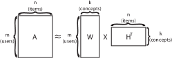
Figure 1: Obtaining $A$.

The matrices $W$ and $H$ are obtained by minimizing the objective function in eq. (1). In this function, $A\in\mathbb{R}^{m\times n}$ is the classification matrix, $m$ is the number of users and $n$ is the number of items.

$$\underset{H\in\mathbb{R}^{n\times k}}{\underset{W\in\mathbb{R}^{m\times k}}{\text{min}}}\sum\limits_{(i,j)\in\Omega}(A_{ij}-\omega^{T}_{i}h_{j})^{2}+\lambda(\lvert\lvert W\rvert\rvert^{2}_{F}+\lvert\lvert H\rvert\rvert^{2}_{F}),$$ (1)

Assuming that the classification matrix is sparse (i.e., a minority of ratings is known), $\Omega$ is the set of indexes related to the observed classifications (ratings), $i$ is the user counter and $j$ is the item counter. The sparse data is represented by the triplet $i,j,classification$. The $\lambda$ parameter is a regularization factor, which determines how precise will be the factorization given by the objective function. In other words, it allows to control the error level and overfitting. The Frobenius norm indicated by $\lvert\lvert\star\rvert\rvert_{F}$, is used to calculate the distance between the matrix $A$ and its approximate matrix $rank-k=A_{k}$. In this context, $E=A-A_{k}$, is the Frobenius norm, which consists of calculating $\lvert\lvert E\rvert\rvert_{F}^{2}=\sum_{i,j}\lvert E_{i,j}\rvert^{2}$. The lower the integer produced by the summation, the nearer is $A$ to $A_{k}$  [13]. The $\omega^{T}_{i}$ vector corresponds to line $i$ of matrix $W$ and the $h_{j}$ vector corresponds to the line $j$ of matrix $H$. Summarizing, the objective function is used to obtain an approximation of the incomplete matrix $A$, where $W$ and $H$ are matrices $rank-k$.

It is not trivial to directly calculate the minimum of the objective function in eq. (1). Therefore, to solve the problem, several methods are used. Next, we explain some of them, most relevant to this work.

3.1 Alternating Least Squares (ALS)

This method divides the minimization function in two quadratic functions. That way, it minimizes $W$ keeping $H$ constant and it minimizes $H$ keeping $W$ constant. When $H$ is constant to minimize $W$, in order to obtain an optimal value to $\omega_{i}^{*}$, the function in eq. (2) is derived.

$$min_{\omega_{i}}\sum\limits_{j\in\Omega_{i}}(A_{ij}-w^{T}_{i}h_{j})^{2}+\lambda\lvert\lvert w_{i}\rvert\rvert^{2}$$ (2)

Next, it is necessary to minimize function in eq. (2). The expression:

$$\omega_{i}^{*}=(H_{\Omega_{i}}^{T}H_{\Omega_{i}}+\lambda I)^{-1}H^{T}a_{i}$$

gives a minimal value for $\omega_{i}^{*}$, given that $\lambda$ is always positive.

The algorithm alternates between the minimizations of $W$ and $H$ until its convergence, or until it reaches a determined number $T$ of iterations, given by the user [17, 19, 20].

In our implementation, the inverse matrix is obtained using the Cholesky decomposition, since it is one of the most efficient methods for matrix inversion [11].

The complete sequential ALS is shown in Algorithm 1.

input : $A,W,H,\lambda,T$

1 Initialize($H\leftarrow\text{(small random numbers)}$);

2 for $iter\leftarrow 1$ to $T$ $Step=1$ do

3      Compute the $W$ using $\omega_{i}^{*}=(H_{\Omega_{i}}^{T}H_{\Omega_{i}}+\lambda I)^{-1}H^{T}a_{i}$;

4      Compute the $H$ using $h_{j}^{*}=(W_{\Omega_{j}}^{T}W_{\Omega_{j}}+\lambda I)^{-1}W^{T}a_{j}$;

5     

Algorithm 1 ALS [17]

3.2 Cyclic Coordinate Descent (CCD)

The algorithm is very similar to ALS, but instead of minimizing function in eq. (1) for all elements of $H$ or $W$, it minimizes the function for each element of $H$ or $W$ at each iteration step [9, 19]. Assuming $\omega_{i}$ represents the line $i$ of $W$, then $\omega_{it}$ represents the element of line $i$ and column $t$. In order to operate element by element, the objective function in eq. (1) needs to be modified such that only $\omega_{it}$ can be assigned a $z$ value. This reduces the problem to a single variable problem, as shown in function in eq. (3).

$$\underset{z}{\text{min}}f(z)=\sum\limits_{j\in\Omega_{i}}(A_{ij}-(\omega^{T}_{i}h_{j}-\omega_{it}h_{jt})-zh_{jt})^{2}+\lambda z^{2},$$ (3)

Given that this algorithm performs a non-negative matrix factorization and function in eq. (3) is invariably quadratic, it has one single minimum. Therefore, it is sufficient to minimize function in eq. (3) in relation to $z$, obtaining eq. (4).

$$z^{*}=\frac{\sum\limits_{j\in\Omega_{i}}(A_{ij}-\omega^{T}_{i}h_{j}+\omega_{it}h_{jt})h_{jt}}{\lambda+\sum\limits_{j\in\Omega_{i}}h^{2}_{jt}},$$ (4)

Finding $z^{*}$ requires $O(\lvert\Omega_{i}\rvert k)$ iterations. If $k$ is large, this step can be optimized after the first iteration, thus requiring only $O(\lvert\Omega_{i}\rvert)$ iterations. In order to do that, it suffices to keep a residual matrix $R$ such that $R_{ij}\equiv A_{ij}-\omega^{T}_{i}h_{j},\forall(i,j)\in\Omega$. Therefore, after the first iteration, and after obtaining $R_{ij}$, the minimization of $z*$ becomes:

$$z^{*}=\frac{\sum\limits_{j\in\Omega_{i}}(R_{ij}+\omega_{it}h_{jt})h_{jt}}{\lambda+\sum\limits_{j\in\Omega_{i}}h^{2}_{jt}},$$ (5)

Having calculated $z^{*}$, the update of $\omega_{it}$ and $R_{ij}$ proceeds as follows:

$$R_{ij}\leftarrow R_{ij}-(z^{*}-\omega_{it})h_{jt},\forall j\in\Omega_{i},$$ (6)

$$\omega_{it}\leftarrow z^{*}.$$ (7)

After updating each variable $\omega_{it}\in W$ using (7), we need to update the variables $h_{jt}\in H$ in a similar manner, obtaining:

$$s^{*}=\frac{\sum\limits_{i\in\bar{\Omega}_{j}}(R_{ij}+\omega_{it}h_{jt})\omega_{it}}{\lambda+\sum\limits_{i\in\bar{\Omega}_{j}}\omega^{2}_{it}},$$ (8)

$$R_{ij}\leftarrow R_{ij}-(s^{*}-h_{jt})\omega_{it},\forall i\in\bar{\Omega}_{j},$$ (9)

$$h_{jt}\leftarrow s^{*}.$$ (10)

Having obtained the updating rules shown in eqs. (6),  (7),  (9) and  (10), we can now apply any sequence of updates to $W$ and $H$. Next, we describe two ways of performing the updates: item/user-wise and feature-wise.

3.2.1 Update item/user-wise CCD

In this type of updating, $W$ and $H$ are updated as in Algorithm 2.

In the first iteration $W$ is initialized with zeros, therefore the residual matrix $R$ is exactly equal to $A$.

input : $A,W,H,\lambda,k,T$

1 initialize($W\leftarrow 0,R\leftarrow A$);

2 for $iter\leftarrow 1$ to $T$ $Step=1$ do

3      for $i\leftarrow 1$ to $m$ $Step=1$ do // $\rhd$ Update $W$.

4          for $t\leftarrow 1$ to $k$ $Step=1$ do

5                obtain $z^{*}$ using (5);

6                update $R$ and $\omega_{it}$ using (6) and (7);

7               

8               

9                for $j\leftarrow 1$ to $n$ $Step=1$ do // $\rhd$ Update $H$.

10                     for $t\leftarrow 1$ to $k$ $Step=1$ do

11                          obtain $s^{*}$ using (8);

12                          update $R$ and $h_{jt}$ using (9) and (10);

13                         

14                         

15                         

Algorithm 2 CCD [19]

3.2.2 Update feature-wise CCD++

Assuming that $\bar{\omega}_{t}$ corresponds to the columns of $W$ and $\bar{h}_{t}$, the columns of $H$, the factorization $WH^{T}$ can be represented as a summation of $k$ outer products.

$$A\approx WH^{T}=\sum\limits_{t=1}^{k}\bar{\omega}_{t}\bar{h}_{t}^{T},$$ (11)

Some modifications need to be made to the original CCD functions. Assuming that $u^{*}$ and $v^{*}$ are the vectors to be injected over $\bar{\omega}_{t}$ and $\bar{h}_{t}$, then $u^{*}$ and $v^{*}$ can be calculated using the following minimization:

$$\underset{u\in\mathbb{R}^{m},v\in\mathbb{R}^{n}}{\text{min}}\sum\limits_{(i,j)\in\Omega}(R_{ij}+\bar{\omega}_{ti}\bar{h}_{tj}-u_{i}v_{j})^{2}+\lambda(\lvert\lvert u\rvert\rvert^{2}+\lvert\lvert v\rvert\rvert^{2}),$$ (12)

$R_{ij}\equiv A_{ij}-\omega^{T}_{i}h_{j},\forall(i,j)\in\Omega$ is the residual entry of $(i,j)$. But using this type of update, there is one more possibility which is to have pre-calculated values using a second residual matrix $\hat{R}_{ij}$:

$$\hat{R}_{ij}=R_{ij}+\bar{\omega}_{ti}\bar{h}_{tj},\forall(i,j)\in\Omega,$$ (13)

This way, the objective function equivalent to (1) is rewritten as:

$$\underset{u\in\mathbb{R}^{m},v\in\mathbb{R}^{n}}{\text{min}}\sum\limits_{(i,j)\in\Omega}(\hat{R}_{ij}-u_{i}v_{j})^{2}+\lambda(\lvert\lvert u\rvert\rvert^{2}+\lvert\lvert v\rvert\rvert^{2}).$$ (14)

To obtain $u^{*}$ it suffices to minimize the function (14) regarding $u_{i}$:

$$u_{i}\leftarrow\frac{\sum\limits_{j\in\Omega_{i}}\hat{R}_{ij}v_{j}}{\lambda+\sum\limits_{j\in\Omega_{i}}v^{2}_{j}},i=1,\ldots,m,$$ (15)

To obtain $v^{*}$ it suffices to minimize (14) regarding $v_{j}$:

$$v_{j}\leftarrow\frac{\sum\limits_{i\in\bar{\Omega}_{j}}\hat{R}_{ij}u_{j}}{\lambda+\sum\limits_{i\in\bar{\Omega}_{j}}u^{2}_{i}},j=1,\ldots,n.$$ (16)

Finally, after obtaining $u^{*}$ e $v^{*}$ we update $(\bar{\omega}_{t},\bar{h}_{t})$ and $R_{ij}$:

$$(\bar{\omega}_{t},\bar{h}_{t})\leftarrow(u^{*},v^{*}),$$ (17)

$$R_{ij}\leftarrow\hat{R}_{ij}-u_{i}^{*}v_{j}^{*},\forall(i,j)\in\Omega,$$ (18)

Algorithm 3 formalizes the feature-wise update of CCD, called CCD++.

input : $A,W,H,\lambda,k,T$

1 initialize($W\leftarrow 0,R\leftarrow A$);

2 for $iter\leftarrow 1$ $\ldots$ $Step=1$ do

3      for $t\leftarrow 1$ to $k$ $Step=1$ do

4           build $\hat{R}$ using (13);

5           for $inneriter\leftarrow 1$ to $T$ $Step=1$ do // $\rhd$ $T$ iterations CCD to (14).

6                update $u$ using (15);

7                update $v$ using (16);

8               

9                update $(\bar{\omega}_{t},\bar{h}_{t})$ and $R$ using (17) and (18);

10               

11               

Algorithm 3 CCD++ [19]

4 Parallel ALS

Parallelizing ALS consists of distributing the matrices $W$ and $H$ among threads. Synchronization is needed as soon as the matrices are updated in parallel [22]. Algorithm 4 shows the modifications related to the sequential ALS algorithm.

input : $A,W,H,\lambda,T$

1 begin

2      Initialize($H\leftarrow\text{(small random numbers)}$);

3      for $iter\leftarrow 1$ to $T$ $Step=1$ do

4           Compute in parallel the $W$ using $\omega_{i}^{*}=(H_{\Omega_{i}}^{T}H_{\Omega_{i}}+\lambda I)^{-1}H^{T}a_{i}$; // Sync ;

5           Compute in parallel the $H$ using $h_{j}^{*}=(W_{\Omega_{j}}^{T}W_{\Omega_{j}}+\lambda I)^{-1}W^{T}a_{j}$; // Sync ;

6          

7          

8          

Algorithm 4 Parallel ALS

5 GPU-ALS

We also parallelized ALS for CUDA. Data are copied to the GPU and the host is responsible for the synchronization. When the computation finishes in the GPU, $W$ and $H$ are copied from the device to the host. Algorithm 5 shows how ALS was parallelized using CUDA.

input : $A,W,H,\lambda,T$

1 Allocate GPU memory for matrices $A$, $W$ and $H$;

2 Copy matrices $A$, $W$ and $H$ from the host to the GPU;

3 begin

4      Intialize($H\leftarrow\text{(small random numbers)}$);

5      for $iter\leftarrow 1$ to $T$ $Step=1$ do

6           Update $W$ using $\omega_{i}^{*}=(H_{\Omega_{i}}^{T}H_{\Omega_{i}}+\lambda I)^{-1}H^{T}a_{i}$; // Host Sync ;

7           Update $H$ using $h_{j}^{*}=(W_{\Omega_{j}}^{T}W_{\Omega_{j}}+\lambda I)^{-1}W^{T}a_{j}$; // Host Sync ;

8          

9           Copy matrices $W$ and $H$ from GPU to host;

10          

11          

Algorithm 5 GPU-ALS

6 Parallel CCD++

In the CCD++ algorithm, each solution is obtained by alternately updating $W$ and $H$. When $v$ is constant, each variable $u_{i}$ is updated independently (eq. 15). Therefore, the update of $u$ can be made by several processing cores.

Given a computer with $p$ cores, we define the partition of the row indexes of $W,\{1,\ldots,m\}$ as $S=S_{1},\ldots,S_{p}$. Vector $u$ is decomposed in $p$ vectors $u^{1},u^{2},\ldots,u^{p}$, where $u^{r}$ is the sub-vector of $u$ corresponding to $S_{r}$. When the matrix $W$ is uniformly split in parts $\lvert S_{1}\rvert=\lvert S_{2}\rvert=\ldots=\lvert S_{p}\rvert=\frac{m}{p}$, there is a load balancing problem due to the variation of the size of the row vectors contained in $W$. In this case, the exact amount of work for each $r$ core to update $u^{r}$ is given by $\sum_{i\in S_{r}}4\lvert\Omega_{i}\rvert$ [19]. Therefore, different cores have different workloads. This is one of the limitations of this algorithm. It can be overcome using dynamic scheduling, which is offered by most parallel processing libraries (e.g. OpenMP [5]).

For each subproblem, each core $r$ builds $\hat{R}$ with,

$$\hat{R}_{ij}\leftarrow R_{ij}+\bar{\omega}_{ti}\bar{h}_{tj},\forall(i,j)\in\Omega_{S_{r}},$$ (19)

where $\Omega_{S_{r}}=\cup_{i\in S_{r}}\{(i,j):j\in\Omega_{i}$. Then, for each core $r$ we have,

$$u_{i}\leftarrow\frac{\sum\limits_{j\in\Omega_{i}}\hat{R}_{ij}v_{j}}{\lambda+\sum\limits_{j\in\Omega_{i}}v^{2}_{j}},\forall i\in S_{r}.$$ (20)

The update of $H$ is analogous to the one of $W$ in (20). For $p$ cores the row indexes of $H,\{1,\ldots,n\}$ are partitioned into $G=G_{1},\ldots,G_{p}$. So, for each core $r$ we have,

$$v_{j}\leftarrow\frac{\sum\limits_{i\in\bar{\Omega}_{j}}\hat{R}_{ij}u_{j}}{\lambda+\sum\limits_{i\in\bar{\Omega}_{j}}u^{2}_{i}},\forall j\in G_{r}.$$ (21)

Since all cores share the same memory, no communication is needed to access $u$ and $v$. After obtaining $(u^{*},v^{*})$, the update of $R$ and $(\bar{\omega}_{t}^{r},\bar{h}_{t}^{r})$ is also implemented in parallel by the $r$ cores as follows.

$$(\bar{\omega}_{t}^{r},\bar{h}_{t}^{r})\leftarrow(u^{r},v^{r}),$$ (22)

$$R_{ij}\leftarrow\hat{R}_{ij}-\bar{\omega}_{ti}\bar{h}_{tj},\forall(i,j)\in\Omega_{S_{r}}.$$ (23)

Algorithm 6 summarizes the parallel CCD operations.

input : $A,W,H,\lambda,k,T$

1 initialize($W\leftarrow 0,R\leftarrow A$);

2 for $iter\leftarrow 1$ $\ldots$ $Step=1$ do

3      for $t\leftarrow 1$ to $k$ $Step=1$ do

4           in parallel, build $\hat{R}$ split by $r$ cores using (19);

5           for $inneriter\leftarrow 1$ to $T$ $Step=1$ do

6                in parallel, update $u$ with $r$ cores using (20);

7                in parallel, update $v$ with $r$ cores using (21);

8               

9                in parallel, update $(\bar{\omega}_{t}^{r},\bar{h}_{t}^{r})$ using (23);

10                in parallel, update $R$ using (23);

11               

12               

13               

Algorithm 6 Multi-core version of CCD++ [19]

7 CCD++ in CUDA

Our CUDA implementation of the CCD++ algorithm uses explicit memory management. It is inspired by the parallel version of CCD++ found in LIBPMF (Library for Large-scale Parallel Matrix Factorization). This is an open source library for Linux [19]. LIBPMF is implemented in C++ for multi-core environments with shared memory. The parallel version uses the OpenMP library [5]. It employs double precision values. Our version uses floats because GPUs are faster when floats are used.

input : $A,W,H,\lambda,k,T$

1 initialize($W\leftarrow 0,R\leftarrow A$);

2 Allocate memory on GPU for matrices $A$ and $R$ and for vectors $u$ and $v$;

3 Copy matrices $A$ and $R$ from host to GPU;

4 for $iter\leftarrow 1$ to $T$ $Step=1$ do

5      for $t\leftarrow 1$ to $k$ $Step=1$ do

6           $u\leftarrow\bar{\omega}_{t}$ and $v\leftarrow\bar{h}_{t}$;

7           Copy vectors $u$ and $v$ from host to GPU;

8           call kernel to update $\hat{R}$ on GPU using (19);

9           for $inneriter\leftarrow 1$ to $T$ $Step=1$ do

10                update $u$ and $v$ on GPU using (20) and (21);

11               

12                Copy vectors $u$ and $v$ from GPU to host;

13                $\bar{\omega}_{t}\leftarrow u$ and $\bar{h}_{t}\leftarrow v$;

14                update $\hat{R}$ on GPU using (23);

15               

16               

Algorithm 7 CCD++ GPU Implementation

Algorithm 7 shows our implementation of the CCD++ for the GPUs.

We use the same stream in all copies from host to device, device to host and for kernels. Therefore, each of the operations is always blocking with respect to the main thread in the host.

8 Materials and Methods

We performed our experiments using two operating systems: Windows 8.1 pro x64 and Linux fedora 20. The CUDA versions for these two systems can vary greatly in performance. The hardware used is described as follows: GPU: Gainward GeForce GTX 580 Phantom, $\approx$ $\$600$, with total dedicated memory 3GB GDDR5 and 512 CUDA Cores; Processors: 2 $\times$ Intel^® Xeon^® X5550, $2\times\$999\approx\$1998$, with 24GB of RAM (6 $\times$ 4GB HYNIX HMT151R7BFR4C-H9); Motherboard: Tyan S7020WAGM2NR.

All experiments use the Netflix dataset (100,480,507 ratings that 480,189 users gave to 17,770 movies). Our qualitative evaluation metric is the root mean squared error (RMSE) produced on the probe data generated by the model. Our quantitative measure is the speedup (how fast it is the parallel implementation related to the sequential, calculated as the sequential execution time divided by the parallel execution time).

Ideally, we needed a secondary GPU with dedicated memory, but this was not possible. In our GPU, the memory is shared with the display memory. We used 16 blocks of 512 threads in our experiments.

The parameters used by both CCD++ and ALS are $k=5$, $\lambda=0.1$ and $T=15$. These were selected according to an empirical selection. Lower values of $k$ give better speedups for the GPU implementation, while a variation of the $k$ values does not impact the multi-core implementation. Higher values of $k$ also implies that more data will be copied to the GPU memory, which is not advisable.

We performed our experiments with two versions of the CCD++, one using float (single decimal precision) and the other using doubles (double decimal precision), in order to evaluate how the GPU would behave with both kinds of numeric types.

All experiments for CCD++ resulted on RMSE equals to $0.94$ and for ALS resulted in RMSE equals to $0.97$.

9 Results and Discussion

Table 1 shows the performance of the original CCD++ (using the library libpmf) on the multi-core machine with Linux and Windows, running the Netflix benchmark, using the original double decimal precision (C double). The speedups achieved in Windows are higher than in Linux, but this was expected, since the base execution of Windows (717.3 s for 1 thread) is higher than the Linux (521.5 s). The maximum speedup achieved is 4.4 with 32 threads.

Table 1: LIBPMF with double in OMP.

OS: Linux
Test	Execution time	Speedup
1 thread	$\pm 521.512s$
2 threads	$\pm 316.701s$	$1.6$
8 threads	$\pm 136.2s$	$3.8$
16 threads	$\pm 126.81s$	$4.1$
32 threads	$\pm 136.023s$	$3.8$
OS: Windows 8.1 pro x64
Test	Execution time	Speedup
1 thread	$\pm 717.307s$
2 threads	$\pm 407.873s$	$1.8$
8 threads	$\pm 179.499s$	$4.0$
16 threads	$\pm 166.746s$	$4.3$
32 threads	$\pm 161.48s$	$4.4$

Table 2 shows the same experiments, but now with our version of CCD++, that uses a single decimal precision. The results are exactly the same in terms of RMSE, but the performance is highly benefited by the numeric data type in this case. By using floats, instead of doubles, we reach speedups of 9.5 (at 32 threads), which is more than twice the speedup achieved with the version that used a double numeric representation. Note that the original libpmf uses doubles instead of floats. We could achieve even better speedups than they reported, by just using single precision data. The use of float or double did not affect much the Linux implementations, but it considerably affected the Windows implementations.

Again, with this version, the Windows implementation achieves higher speedups than Linux. This was expected, since the base execution time for 1 thread is much higher for Windows.

Table 2: CCD++ with float in OMP and CUDA.

OS: Linux
Test	Execution time	Speedup
1 thread	$\pm 528.538s$
2 threads	$\pm 309.707s$	$1.7$
8 threads	$\pm 111.968s$	$4.7$
16 threads	$\pm 98.1266s$	$5.3$
32 threads	$\pm 99.8027s$	$5.2$
CUDA	$\pm\textbf{168.109s}$	3.1
OS: Windows 8.1 pro x64
Test	Execution time	Speedup
1 thread	$\pm 1252.35s$
2 threads	$\pm 540.973s$	$2.3$
8 threads	$\pm 181.501s$	$6.9$
16 threads	$\pm 131.881s$	$9.5$
32 threads	$\pm 131.661s$	$9.5$
CUDA	$\pm\textbf{84.7718s}$	14.8

But our best results are for the CUDA implementation. We obtained a speedup of 14.8 just using the GPU running our implementation of the CCD++ in Windows. We managed to surpass the performance of a machine that costs more than twice as much as a GPU card, showing that these architectures have a great potential for the implementation of recommender systems based on matrix factorization.

9.1 ALS

Table 3: ALS with float in OMP and CUDA.

OS: Linux
Test	Execution time	Speedup
1 thread	$\pm 429.539s$
2 threads	$\pm 224.99s$	$1.9$
8 threads	$\pm 93.8716s$	$4.6$
16 threads	$\pm 98.3057s$	$4.3$
32 threads	$\pm 95.8294s$	$4.5$
CUDA	$\pm\textbf{98.71s}$	4.4
OS: Windows 8.1 pro x64
Test	Execution time	Speedup
1 thread	$\pm 665.74s$
2 threads	$\pm 355.144s$	$1.9$
8 threads	$\pm 158.912s$	$4.2$
16 threads	$\pm 121.667s$	$5.5$
32 threads	$\pm 122.121s$	$5.5$
CUDA	$\pm\textbf{107.214s}$	6.2

We also implemented the ALS algorithm in CUDA and results are presented in Table 3 for comparison. In this table we show execution times and speedups for the multi-core version and for the GPU. Once more the multi-core version presents better speedups with a higher number of threads, for the Windows environment.

10 Conclusions

We showed the advantage of using GPUs to implement recommender systems based on matrix factorization algorithms. Using a benchmark popular in the literature, Netflix, we obtained maximum speedup of 14.8, better than the best speedup reported in the literature.

The advantages of using a CUDA implementation over a multi-core server are: lower energy consumption, lower price and the ability of leaving the main host or other cores to be used by other tasks. Currently, almost every computer comes with PCI slots that can be used to install a GPU or various GPUs. Thus, it is relatively simple to expand the computational capacity of an existing hardware.

We plan to perform more tests with our algorithms on more recent GPUs and on larger datasets. One potential problem of GPUs is their memory limitation. Therefore, one path to follow is to implement efficient memory management mechanisms capable of dealing with bigger data. Another track we would like to follow is to implement a load balancing mechanism to these algorithms.

11 Acknowledgments

National Funds through the FCT - Fundação para a Ciência e a Tecnologia (proj. FCOMP-01-0124-FEDER-037281).

1cm

References

- [1] H. Andrews and C. Patterson. Singular value decompositions and digital image processing. Acoustics, Speech and Signal Processing, IEEE Transactions on, 24(1):26–53, Feb 1976.
- [2] E.-A. Baatarjav, S. Phithakkitnukoon, and R. Dantu. Group recommendation system for facebook. In Proceedings of the OTM Confederated International Workshops and Posters on On the Move to Meaningful Internet Systems, OTM ’08, pages 211–219, Berlin, Heidelberg, 2008. Springer-Verlag.
- [3] O. Bretscher. Linear Algebra With Applications. Pearson Education, Boston, 2013.
- [4] R. Burke. The adaptive web. In P. Brusilovsky, A. Kobsa, and W. Nejdl, editors, Lecture Notes In Computer Science, Vol. 4321., chapter Hybrid Web Recommender Systems, pages 377–408. Springer-Verlag, Berlin, Heidelberg, 2007.
- [5] R. Chandra. Parallel Programming in OpenMP. High performance computing. Morgan Kaufmann, 2001.
- [6] J. Fang, A. L. Varbanescu, and H. Sips. A comprehensive performance comparison of cuda and opencl. In Proceedings of the 2011 International Conference on Parallel Processing, ICPP ’11, pages 216–225, Washington, DC, USA, 2011. IEEE Computer Society.
- [7] J. He. A Social Network-based Recommender System. PhD thesis, UCLA, Los Angeles, CA, USA, 2010. AAI3437557.
- [8] R. Hochberg. Matrix multiplication with cuda-a basic introduction to the cuda programming model. Shodor, 2012.
- [9] C.-J. Hsieh and I. S. Dhillon. Fast coordinate descent methods with variable selection for non-negative matrix factorization. In Proceedings of the 17th ACM SIGKDD, KDD ’11, pages 1064–1072, New York, NY, USA, 2011. ACM.
- [10] Y. Koren and R. Bell. Advances in collaborative filtering. In F. Ricci, L. Rokach, B. Shapira, and P. B. Kantor, editors, Recommender Systems Handbook, pages 145–186. Springer US, 2011.
- [11] A. Krishnamoorthy and D. Menon. Matrix inversion using cholesky decomposition. In Signal Processing: Algorithms, Architectures, Arrangements, and Applications (SPA), 2013, pages 70–72, Sept 2013.
- [12] T. Mahmood and F. Ricci. Improving recommender systems with adaptive conversational strategies. In Proceedings of the 20th ACM Conference on Hypertext and Hypermedia, HT ’09, pages 73–82, New York, NY, USA, 2009. ACM.
- [13] C. D. Meyer, editor. Matrix Analysis and Applied Linear Algebra. Society for Industrial and Applied Mathematics, Philadelphia, PA, USA, 2000.
- [14] P. Resnick and H. R. Varian. Recommender systems. Commun. ACM, 40(3):56–58, Mar. 1997.
- [15] J. Sanders and E. Kandrot. CUDA by Example: An Introduction to General-Purpose GPU Programming. Addison-Wesley Professional, 1st edition, 2010.
- [16] B. M. Sarwar, G. Karypis, J. A. Konstan, and J. T. Riedl. Application of dimensionality reduction in recommender system – a case study. In IN ACM WEBKDD WORKSHOP, 2000.
- [17] G. Takács and D. Tikk. Alternating least squares for personalized ranking. In Proceedings of the Sixth ACM Conference on Recommender Systems, RecSys ’12, pages 83–90, New York, NY, USA, 2012. ACM.
- [18] N. Wilt. The CUDA Handbook: A Comprehensive Guide to GPU Programming. Pearson Education, 2013.
- [19] H.-F. Yu, C.-J. Hsieh, S. Si, and I. Dhillon. Parallel matrix factorization for recommender systems. Knowledge and Information Systems, pages 1–27, 2013.
- [20] D. Zachariah, M. Sundin, M. Jansson, and S. Chatterjee. Alternating least-squares for low-rank matrix reconstruction. Signal Processing Letters, IEEE, 19(4):231–234, April 2012.
- [21] G. Zhanchun and L. Yuying. Improving the collaborative filtering recommender system by using gpu. In Cyber-Enabled Distributed Computing and Knowledge Discovery (CyberC), 2012 International Conference on, pages 330–333, Oct 2012.
- [22] Y. Zhou, D. Wilkinson, R. Schreiber, and R. Pan. Large-scale parallel collaborative filtering for the netflix prize. In Proc. 4th Int’l Conf. Algorithmic Aspects in Information and Management, LNCS 5034, pages 337–348. Springer, 2008.
- [23] M. A. Zinkevich, A. Smola, M. Weimer, and L. Li. Parallelized stochastic gradient descent. In Advances in Neural Information Processing Systems 23, pages 2595–2603, 2010.