Globally solving Non-Convex Quadratic Programs via Linear Integer Programming techniques

Abstract

Quadratic programming (QP) is a well-studied fundamental NP-hard optimization problem which optimizes a quadratic objective over a set of linear constraints. In this paper, we reformulate QPs as a mixed-integer linear problem (MILP). This is done via the reformulation of QP as a linear complementary problem, and the use of binary variables and big-M constraints, to model the complementary constraints. To obtain such reformulation, we show how to impose bounds on the dual variables without eliminating all the (globally) optimal primal solutions; using some fundamental results on the solution of perturbed linear systems.

Reformulating non-convex QPs as MILPs provides an advantageous way to obtain global solutions as it allows the use of current state-of-the-art MILP solvers. To illustrate this, we compare the performance of our solution approach, labeled quadprogIP, with the current benchmark global QP solver quadprogBB, as well as with BARON, one of the leading non-linear programming (NLP) solvers, and CPLEX’s non-convex QP solver, on a large variety of QP test instances. In practice, quadprogIP is shown to typically outperform by orders of magnitude quadprogBB, BARON, and CPLEX on standard QPs. For general QPs, quadprogIP outperforms quadprogBB, outperforms BARON in most instances, while CPLEX performs the best on these instances. For box-constrained QPs, quadprogIP has a comparable performance to quadprogBB and BARON in small- to medium-scale instances, but is outperformed by these solvers on large-scale instances; while CPLEX performs the best on box-constrained QP instances. Also, unlike quadprogBB, the solution approach proposed here is able to solve QP instances whose dual feasible set is unbounded. The MATLAB code, called quadprogIP, and the instances used to perform these numerical experiments are publicly available at https://github.com/xiawei918/quadprogIP.

1 Introduction

Quadratic programmming (QP), is a fundamental optimization problem with a quadratic objective and linear constraints. QP is NP-hard (see, e.g., Pardalos and Vavasis 1991, and the references therein), however, when the objective is convex, QP can be globally solved (within a predetermined precision $\epsilon>0$) in polynomial time via interior-point methods (see, e.g., Renegar 2001). Here, the focus is on obtaining global solutions for non-convex QP. QP is arguably the most basic instance of a (non-convex), non-linear program (NLP). At a fundamental level, the complexity of globally solving QP lies in the fact that multiple of its local optimal solutions may not necessarily be global optimal solutions (see, e.g. Bertsekas 1999).

QPs commonly arise in applications in engineering, pure and social sciences, finance, and economics (see, e.g., Horst et al. 2000). As a result, there has been extensive work on studying how to obtain global solutions of QPs using both NLP techniques (see, Gould et al. 2003, Gao 2004, for surveys in this area), and convex optimization techniques (consider, e.g., Nesterov 1998, Kim and Kojima 2001, 2003, Chen and Burer 2012, among many others).

In this paper, we reformulate QPs as a mixed-integer linear problem (MILP). This provides an advantageous way to obtain global solutions as it allows the use of current state-of-the-art MILP solvers. Moreover, the numerical experiments of Section 3 show that a basic implementation of the proposed algorithm, which we refer to as quadprogIP, typically outperform by orders of magnitude quadprogBB, BARON, and CPLEX on standard QPs. For general QPs, quadprogIP outperforms quadprogBB, outperforms BARON in most instances, while CPLEX performs the best on these instances. For box-constrained QPs, quadprogIP has a comparable performance to quadprogBB and BARON in small- to medium-scale instances, but is outperformed by these solvers on large-scale instances; while CPLEX performs the best on box-constrained QP instances.

Unlike quadprogBB, the solution approach proposed here is able to solve QP instances whose dual feasible set is unbounded. The MATLAB code and the instances used to perform these numerical experiments are available at https://github.com/xiawei918/quadprogIP.

To obtain the proposed MILP-reformulation (see Sec. 2.1), the QP’s KKT conditions are used to reformulate the QP as a linear complementarity problem (LCP). In this reformulation, the complexity of the problem is captured by the complementarity constraints. The KKT-branching approach (Burer and Vandenbussche 2009), which consist on branching on this complementarity constraints, is not useful on this reformulation of the problem, as the underlying linear relaxations at the root node of the KKT-branching tree are (under mild assumptions) unbounded (Burer and Vandenbussche 2009, Cor. 2.3). Another alternative, namely, reformulating the complementarity constraints using binary variables and big M constraints, requires the knowledge of bounds on the problem’s KKT multipliers, which in general are unbounded (cf., Hu et al. 2012, Sec. 6.1 and 6.2). To directly use MILP solvers for the solution of the QP, we overcome this requirement by restricting our attention to a subset of optimal KKT points. We show (Theorem 1) that it is possible to impose bounds on the dual variables without eliminating all the (globally) optimal primal solutions. Our results are based on fundamental results on the approximate solution of systems of linear equations (e.g., Güler et al. 1995, Mangasarian 1981). One advantage of the proposed methodology is that unlike previous related work, the convergence of the MILP-based approach to the QP’s global optimal solution in finite time follows in straightforward fashion (see Sec. 3.1.1). Also, the methodology can be applied to QPs without the need for assumptions on the relative interior of its feasible set (see Sec. 2.3 for details).

Before stating the results described above, we end this section with a short review of both NLP and convex optimization techniques for the global solution of QP’s. Using NLP techniques, Vanderbei and Shanno (1999) proposed an interior-point algorithm for NLPs (thus, applicable for QPs), which is an extension of the interior-point methods for linear and convex optimization problems (cf., Renegar 2001). Floudas and Visweswaran (1990) proposed an algorithm which globally solves certain classes of NLPs by decomposing the problem based on an appropriate partition of its decision variables. The work of Belotti et al. (2009) and Tawarmalani and Sahinidis (2004) on the use of relaxation and linearization techniques (cf., Sherali and Adams 1994), in combination with spatial branching techniques (cf., Tawarmalani and Sahinidis 2004), has lead to the development of the two well-known global solvers Couenne (Belotti 2010) and BARON (Sahinidis 1996) for NLPs. Another solver that combines these type of techniques, together with techniques to exploit the problems structure is GloMIQO, developed by Misener and Floudas (2013) for the solution of more general quadratically constrained quadratic programs with integer variables. More recently, specialized solution approaches have been developed for special classes of QP. In particular, Bonami et al. (2016b) develop a special branch-and-cut algorithm for box constrained QPs based on using cuts derived from the boolean quadric polytope. Also, Bonami et al. (2016a) develop new specialized cuts that are used within a spatial branch and bound algorithm to solve standard QPs. For further review of numerical and theoretical results on the solution of QPs using NLP techniques, we refer the reader to Gould et al. (2003) and Gao (2004).

Besides NLP techniques, convex optimization techniques (cf., Renegar 2001, Ben-Tal and Nemirovski 2001) have also been used to address the solution of QPs. For example, Nesterov (1998) and later Kim and Kojima (2001, 2003), explored the use of semidefinite programming (SDP) as well as second-order cone relaxations to approximately or globally solve a QP.

More recently, Burer and Vandenbussche (2009) proposed a SDP-based branch and bound approach to globally solve box-constrained QPs; they reformulate a QP by adding the QP’s corresponding Karush-Kuhn-Tucker (KKT) conditions as redundant constraints. Let us refer to this quadratically constrained quadratic program (QCQP) as $\operatorname{QP_{\rm KKT}}$. To solve $\operatorname{QP_{\rm KKT}}$, Burer and Vandenbussche (2009) construct a finite KKT-branching tree by branching on the resulting problem’s complementarity constraints. SDP relaxations of $\operatorname{QP_{\rm KKT}}$ are used to obtain lower bounds at each node of the KKT-branching tree. On the other hand, to obtain upper bounds a (local) QP-solver based on NLP techniques is used. Chen and Burer (2012) improved the solution methodology of Burer and Vandenbussche (2009) by obtaining tighter lower bounds at each node of the KKT-branching tree. For that purpose, the double non-negative (DNN) relaxation of the completely positive reformulation (Burer 2009) of $\operatorname{QP_{\rm KKT}}$ at each node of the KKT-branching tree is used. Chen and Burer (2012) provide a MATLAB implementation of their approach called quadprogBB. In this implementation, the MATLAB (local) QP solver quadprog is used to obtain the upper bounds while the algorithm proposed by Burer (2010) is used to obtain lower bounds, at each node of the KKT-branching tree. Chen and Burer (2012) show that this solution approach typically outperforms the solver Couenne and the approach proposed by Burer and Vandenbussche (2009) on a test bed of publicly available QP instances. This makes the solver quadprogBB a current benchmark for the global solution of QP problems.

The rest of the paper is organized as follows. In Section 2, we formally introduce the QP problem and present the theoretical results that serve as the foundation for the proposed solution approach. In Section 3, we illustrate the effectiveness of this approach by presenting relevant numerical results on test instances of the QP problem. To conclude, in Section 4, we provide conclusions and directions for future work.

2 Solution Approach for non-convex QPs

We consider the following quadratic programming problem

$$\begin{array}[]{rrl}{\rm QP:}&\min&\frac{1}{2}x^{\intercal}Hx+f^{\intercal}x\\ &\operatorname{s.t.}&Ax=b\\ &&x\geq 0,\end{array}$$ (1)

where $f\in{\mathbb{R}}^{n}$, $A\in{\mathbb{R}}^{m\times n}$, $b\in{\mathbb{R}}^{m}$, and $H\in{\mathbb{R}}^{n\times n}$ is a symmetric matrix. Note that there is no assumption on the matrix $H$ being positive semidefinite; that is, QP is in general a non-convex optimization problem (cf., Bertsekas 1999).

Similar to Burer and Vandenbussche (2009) and Chen and Burer (2012), we assume that the feasible set of QP is nonempty and bounded. However, in what follows, no further assumption is made about the feasible set of QP.

2.1 Mixed-integer linear programming reformulation

After introducing the Lagrange multipliers $\mu\in{\mathbb{R}}^{m}$ for its equality constraints and $\lambda\in{\mathbb{R}}^{n}$ for its non-negativity constraints, the KKT conditions for QP are given by

$$Hx+f+A^{\intercal}\mu-\lambda =0$$ (2a)

$$x^{\intercal}\lambda =0$$ (2b)

$$Ax =b$$ (2c)

$$x\geq 0,\lambda \geq 0.$$ (2d)

In what follows, we will refer to the set

$$\Lambda_{KKT}=\{(x,\mu,\lambda)\in{\mathbb{R}}^{2n+m}:(x,\mu,\lambda)\text{ satisfy}~{}\eqref{LKKT}-\eqref{nonNegKKT}\}$$ (3)

as the KKT points of QP.

Note that because the feasible set of QP (1) is a polyhedron, the KKT conditions (2) are first order necessary conditions for the optimal solutions of QP (see, e.g. Eustaquio et al. 2008, Thm. 3.3). Thus, one can add these KKT conditions as redundant constraints in QP to obtain the following equivalent formulation of QP,

$$\begin{array}[]{rll}\min&\frac{1}{2}x^{\intercal}Hx+f^{\intercal}x\\ \operatorname{s.t.}&Hx+f+A^{\intercal}\mu-\lambda&=0\\ &x^{\intercal}\lambda=0\\ &Ax=b\\ &x\geq 0,\lambda\geq 0.\\ \end{array}$$ (4)

As shown by Giannessi and Tomasin (1973, Thm. 2.4), one can use the KKT conditions (2a)–(2c) to linearize the objective of (4). Namely, for any feasible solution $x\in{\mathbb{R}}^{n}$ of (4), we have

$$\frac{1}{2}x^{\intercal}Hx+f^{\intercal}x=\frac{1}{2}(f^{\intercal}x-x^{\intercal}A^{\intercal}\mu+x^{\intercal}\lambda)=\frac{1}{2}(f^{\intercal}x-b^{\intercal}\mu).$$ (5)

As a result, problem (4) is equivalent to the following problem with a linear (instead of quadratic) objective.

$$\begin{array}[]{rll}\frac{1}{2}\min&f^{\intercal}x-b^{\intercal}\mu\\ \operatorname{s.t.}&Hx+f+A^{\intercal}\mu-\lambda&=0\\ &x^{\intercal}\lambda=0\\ &Ax=b\\ &x\geq 0,\lambda\geq 0.\\ \end{array}$$ (6)

Notice that in (6), the complexity of QP is captured in the complementary constraints $x^{\intercal}\lambda=0$. Next, we address the complementary constraints in (6) by using Big-M constraints. For that purpose, in Section 2.2, we derive upper bounds $U,V\in{\mathbb{R}}^{n}$ on the decision variables $x,\lambda\in{\mathbb{R}}^{n}$ of (6) such that there are (globally) optimal KKT points $(x,\mu,\lambda)\in{\mathbb{R}}^{2n+m}$ of  QP satisfying $x\leq U$, $\lambda\leq V$. Using these upper bounds, one can show (see, Theorem 1) that a global optimal solution of QP can be obtained by solving the following MILP

$$\begin{array}[]{rllll}{\rm IQP:}\qquad\qquad\qquad\frac{1}{2}\min&f^{\intercal}x-b^{\intercal}\mu\\ \operatorname{s.t.}&Hx+f+A^{\intercal}\mu-\lambda=0\\ &Ax=b\\ &0\leq x_{j}\leq z_{j}U_{j}&j=1,\dots,m\\ &0\leq\lambda_{j}\leq(1-z_{j})V_{j}&j=1,\dots,m\\ &z_{j}\in\{0,1\}&j=1,\dots,m.\end{array}$$ (7)

Specifically, problem IQP is a MILP with the same optimal value as QP whose optimal solutions are optimal solutions of QP.

2.2 Bounding the primal and dual variables

As mentioned earlier, the first step in obtaining problem IQP is to derive explicit upper bounds $U,V\in{\mathbb{R}}^{n}$ such that there are optimal KKT points $(x,\mu,\lambda)\in{\mathbb{R}}^{2n+m}$ of QP satisfying $x\leq U$, $\lambda\leq V$.

Similar to Chen and Burer (2012), using the assumption that the feasible set of QP is non-empty and bounded, one can compute the upper bounds $U\in{\mathbb{R}}^{n}_{+}$ on the primal variables $x\in{\mathbb{R}}^{n}$ by setting:

$$U_{j}:=\max\{x_{j}:Ax=b,\,x\geq 0\},$$ (8)

for every $j=1,\dots,n$.

Using assumptions stronger than ours, Chen and Burer (2012) show that $\Lambda_{KKT}$, the set of KKT points, is bounded. As the following example illustrates, under our weaker assumptions, the set $\Lambda_{KKT}$ could be unbounded.

Example 1.

Consider the instance of QP defined by setting

$$H={\begin{bmatrix}2&0&0\\ 0&-1&0\\ 0&0&1\end{bmatrix}}\qquad f={\begin{bmatrix}2\\ 4\\ 3\end{bmatrix}}\qquad A={\begin{bmatrix}2&1&1\\ 1&1&1\end{bmatrix}}\qquad b=\begin{bmatrix}1\\ 1\end{bmatrix}.$$

Note that in this case the feasible region of QP is $\{[0,1-t,t]^{\intercal}:0\leq t\leq 1\}$, which is bounded and non-empty. However, the set of KKT points $\Lambda_{KKT}$ (3) is unbounded. Specifically, notice that for any $v\geq 1$ the following is a KKT point for QP :

$$x={\small\begin{bmatrix}0\\ 1\\ 0\end{bmatrix}}\qquad\mu={\small\begin{bmatrix}v\\ -3-v\end{bmatrix}}\qquad\lambda={\small\begin{bmatrix}-1+v\\ 0\\ 0\end{bmatrix}}.$$

Thus, to handle the complementarity contrains in (6) using Big-M constraints, we do not try to obtain a bound for the value of the entries of $\lambda\in{\mathbb{R}}^{m}$ for all KKT points. Instead, in Theorem 1, we prove that there exist a bound that we can impose in the dual variables, without discarding all (globally) optimal KKT points of QP. For this purpose, we make use of fundamental results on the approximate solution of systems of linear equations (e.g., Güler et al. 1995, Mangasarian 1981).

Let us first define a particular instance of the well-known Hoffman bound (Hoffman 2003), closely following the notation in Güler et al. (1995).

Definition 1.

Fix the norm $\|\cdot\|_{\alpha}$ on ${\mathbb{R}}^{n}$ and the norm $\|\cdot\|_{\beta}$ on ${\mathbb{R}}^{m}$. Given $A\in{\mathbb{R}}^{m\times n}$ and $b\in{\mathbb{R}}^{m}$, let $F:=\{x\in{\mathbb{R}}^{n}_{+}:Ax=b\}$. Let $\mathcal{H}_{A,b}\in{\mathbb{R}}$ be the smallest constant satisfying:

$$\text{For all }y\in{\mathbb{R}}^{n}\text{ such that }Ay=b,\text{ there is }x\in F\text{ such that }\|x-y\|_{\alpha}\leq\mathcal{H}_{A,b}\|y^{-}\|_{\beta}.$$ (9)

Above, for any $y\in{\mathbb{R}}^{n}$, $y^{-}\in{\mathbb{R}}^{n}$ is the vector difined by $y^{-}_{i}=\max\{0,-y_{i}\}$, $i=1,\dots,n$. That is, Definition 1 corresponds to the Hoffman bound obtained when looking at perturbations of only the non-negative constraints of the polyhedron $F:=\{x\in{\mathbb{R}}^{n}_{+}:Ax=b\}$.

In what follows we will use the following notation to denote the dual norm associated to a given norm.

Definition 2.

Given a norm $\|\cdot\|$ on ${\mathbb{R}}^{n}$, its associated dual norm on ${\mathbb{R}}^{n}$, denoted $\|\cdot\|^{*}$ is defined as:

$$\|x\|^{*}=\sup\{x^{\intercal}z:z\in{\mathbb{R}}^{n},\,\|z\|\leq 1\}.$$

In particular, for any $x\in{\mathbb{R}}^{n}$, $\|x\|_{\infty}^{*}=\|x\|_{1}$.

Using Definition 1, we provide in Theorem 1 below, the desired bound to be used on the dual variables of QP in the IQP formulation (7).

Theorem 1.

Let $A\in{\mathbb{R}}^{m\times n}$ and $b\in{\mathbb{R}}^{m}$ be such that the set $F:=\{x\in{\mathbb{R}}^{n}_{+}:Ax=b\}$ is non-empty and bounded. Let $\mathcal{H}_{A,b}$ be defined by (9), and $M>(\kappa+\|f\|_{\alpha}^{*})\mathcal{H}_{A,b}\|e\|_{\beta}$, where $\kappa:=\max\{\|Hx\|^{*}_{\alpha}:Ax=b,x\geq 0\}$. Then, there exists an optimal KKT point $(x^{*},\mu^{*},\lambda^{*})$ for QP such that $e^{\intercal}\lambda^{*}\leq M$, and $\mu^{*}\in{\mathbb{R}}^{m}$.

Proof.

Proof. Consider the following perturbed version of QP:

$$\begin{array}[]{ll}\min&\frac{1}{2}x^{\intercal}Hx+f^{\intercal}x+Mt\\ \operatorname{s.t.}&Ax=b\\ &x\geq-te\\ &0\leq t\leq\delta,\\ \end{array}$$ (10)

where $e$ is the vector of all ones, and $\delta>0$. Notice that the feasible set of (10) is a closed subset of $\{x\in{\mathbb{R}}^{n}:Ax=b,\,x\geq-\delta e\}\times[0,\delta]$ which is non-empty and bounded as $F$ is non-empty, bounded, and the recession cone of $\{x\in{\mathbb{R}}^{n}:Ax=b,\,x\geq-\delta e\}$ is equal to the recession cone of $F$. Thus, the optimal value of (10) exists and it is attained.

Let $(x^{*},t^{*})$ be an optimal solution of (10). Then, there exists $(\mu^{*},\lambda^{*},\rho^{*},\omega^{*})\in{\mathbb{R}}^{n+m+2}$ such that $(x^{*},t^{*},\mu^{*},\lambda^{*},\rho^{*},\omega^{*})$ satisfies the KKT conditions associated with problem (10)

$$\begin{array}[]{rllll}Hx^{*}+f+A^{\intercal}\mu^{*}-\lambda^{*}&=0\\ M-e^{\intercal}\lambda^{*}-\rho^{*}+\omega^{*}&=0\\ (x^{*}-t^{*}e)^{\intercal}\lambda^{*}&=0\\ {t^{*}}\rho^{*}&=0\\ (\delta-t^{*})\omega^{*}&=0\\ Ax^{*}&=b\\ x^{*}+t^{*}e&\geq 0\\ 0\leq t^{*}&\leq\delta\\ \lambda^{*},\rho^{*},\omega^{*}&\geq 0,\end{array}$$ (11)

where $\mu^{*}\in{\mathbb{R}}^{m}$, $\lambda^{*}\in{\mathbb{R}}^{n}$, $\rho^{*}\in{\mathbb{R}}$, $\omega^{*}\in{\mathbb{R}}$, are respectively the Lagrangian multipliers of problem (10) associated with the linear constraints, lower bounds in the decision variables $x\in{\mathbb{R}}^{n}$, and lower and upper bounds on the decision variable $t\in{\mathbb{R}}$.

Now we claim that $t^{*}=0$. In that case, notice that the complementarity constraint $(\delta-t^{*})\omega^{*}=0$ in (11) implies $\omega^{*}=0$ and thus, from the equation $M-e^{\intercal}\lambda^{*}-\rho^{*}+\omega^{*}=0$ in (11) and the fact that $\rho^{*}\geq 0$, it follows that $(x^{*},\mu^{*},\lambda^{*})$ satisfies the statement of the theorem.

To show that $t^{*}=0$, note that from Definition 1, it follows that there exists $x^{\prime}\in F$ such that

$$\|x^{\prime}-x^{*}\|_{\alpha}\leq\mathcal{H}_{A,b}t^{*}\|e\|_{\beta}.$$ (12)

In problem (10), $(x^{\prime},0)$ is a feasible solution and thus the objective value of $(x^{\prime},0)$ is no smaller than the objective value of $(x^{*},t^{*})$. That is,

$$\frac{1}{2}{x^{*}}^{\intercal}Hx^{*}+f^{\intercal}x^{*}+Mt^{*}\leq\frac{1}{2}{x^{\prime}}^{\intercal}Hx^{\prime}+f^{\intercal}x^{\prime}.$$ (13)

Therefore,

$$Mt^{*} \leq\frac{1}{2}({x^{\prime}}^{\intercal}Hx^{\prime}-{x^{*}}^{\intercal}Hx^{*})+f^{\intercal}(x^{\prime}-x^{*})$$

$$=\frac{1}{2}(x^{\prime}+x^{*})^{\intercal}H(x^{\prime}-x^{*})+f^{\intercal}(x^{\prime}-x^{*})$$

$$\leq\frac{1}{2}\|H(x^{\prime}+x^{*})\|^{*}_{\alpha}\|x^{\prime}-x^{*}\|_{\alpha}+\|f\|_{\alpha}^{*}\|x^{\prime}-x^{*}\|_{\alpha}$$

$$\leq\left(\frac{1}{2}(\|Hx^{\prime}\|^{*}_{\alpha}+\|Hx^{*}\|^{*}_{\alpha})+\|f\|_{\alpha}^{*}\right)\|x^{\prime}-x^{*}\|_{\alpha}.$$

Thus, using (12) we have

$$Mt^{*}\leq\left(\frac{1}{2}(\kappa+\kappa_{\delta})+\|f\|_{\alpha}^{*}\right)\mathcal{H}_{A,b}\|e\|_{\beta}t^{*}$$ (14)

where $\kappa_{\delta}:=\max\{\|Hx\|^{*}_{\alpha}:Ax=b,x\geq-\delta e,x\in{\mathbb{R}}^{n}\}$.

As $M>\left(\kappa+\|f\|_{\alpha}^{*}\right)\mathcal{H}_{A,b}\|e\|_{\beta}$, and $\kappa_{\delta}\downarrow\kappa$ when $\delta\downarrow 0$, taking $\delta>0$ small enough we have that $M>\left(\frac{1}{2}(\kappa+\kappa_{\delta})+\|f\|_{\alpha}^{*}\right)\mathcal{H}_{A,b}\|e\|_{\beta}$. Thus, (14) implies that $t^{*}=0$.∎

2.3 Computation of the dual bounds

Theorem 1 provides the bounds needed for the reformulation of QP as IQP (7) in terms of the Hoffman constant $\mathcal{H}_{A,b}$ introduced in Definition 1. Next, we discuss how this constant can be obtained in closed-form for important special classes of QP, as well as how it can be computed for general classes of QP.

2.3.1 Standard Quadratic Programming.

Consider the standard quadratic program (SQP):

$$\begin{array}[]{llllll}{\rm SQP:}\quad\quad\quad\displaystyle\max_{x\in\Delta}&\frac{1}{2}x^{\intercal}Hx+f^{\intercal}x\\ \end{array}$$ (15)

where $\Delta=\left\{x\in\mathbb{R}^{n}:\sum_{i=1}^{n}x_{i}=1,x\geq 0\right\}$, is the standard simplex. The SQP problem is fundamental in optimization and arises in many applications (see, e.g., Bomze 1998). Next, we show that in this case, the Hoffman bound $\mathcal{H}_{A,b}$ introduced in Definition 1 can be computed in closed-form for suitable choices of the norm $\|\cdot\|_{\alpha}$ on ${\mathbb{R}}^{n}$ and the norm $\|\cdot\|_{\beta}$ on ${\mathbb{R}}^{m}$.

Proposition 1.

Consider the norm $\|\cdot\|_{\alpha}=\|\cdot\|_{1}$ on ${\mathbb{R}}^{n}$ and the norm $\|\cdot\|_{\beta}=\|\cdot\|_{1}$ on ${\mathbb{R}}^{m}$. Let $A=e^{\intercal}$ and $b=1$. Then $\mathcal{H}_{A,b}=2$.

Proof.

Proof. Let $y\in{\mathbb{R}}^{n}$ such that $e^{\intercal}y=1$ be given. Let $I=\{i\in\{1,\dots,n\}:y_{i}\geq 0\}$ and $I^{c}=\{1,\dots,n\}\setminus I$, and consider the case $I^{c}\neq\emptyset$ (otherwise, the statement follows by letting $x=y$ in Definition 1). Note that $e^{\intercal}y=1$ implies $I\not=\emptyset$ and that $\sum_{i\in I}y_{i}=1-\sum_{i\in I^{c}}y_{i}=1+\|y^{-}\|_{1}$. Let $x\in{\mathbb{R}}^{n}$ be defined by setting $x_{i}=0$ for all $i\in I^{c}$, and $x_{i}=\frac{1}{1+\|y^{-}\|_{1}}y_{i}$ for all $i\in I$. Clearly, $x\in\Delta$. Furthermore, for any $i\in I^{c}$, $|x_{i}-y_{i}|=-y_{i}$. Also for any $i\in I$, we have $|x_{i}-y_{i}|=\frac{\|y^{-}\|_{1}}{1+\|y^{-}\|_{1}}y_{i}$. Thus, $\|x-y\|_{1}=-\sum_{i\in I^{c}}y_{i}+\frac{\|y^{-}\|_{1}}{1+\|y^{-}\|_{1}}\sum_{i\in I}y_{i}=2\|y^{-}\|_{1}$. That is, $\mathcal{H}_{A,b}\leq 2$. To show $\mathcal{H}_{A,b}\geq 2$, consider $y=(n,-1,\dots,-1)$. For any $x\in\Delta$, it follows that $\|x-y\|_{1}=|x_{1}-n|+\sum_{i=2}^{n}|x_{i}+1|=2n-1-x_{1}+\sum_{i=2}^{n}x_{i}=2(n-x_{1})\geq 2(n-1)=2\|y^{-}\|_{1}$. ∎

Thus, (15) can be reformulated as IQP by letting:

$$U=e\text{ and }V>Me,$$ (16)

with

$$M=2n\left(\|H\|_{\infty,\infty}+\|f\|_{\infty}\right),$$ (17)

where we have used that

$$\kappa=\max\{\|Hx\|_{\infty}:e^{\intercal}x=1,x\in{\mathbb{R}}^{n}_{+}\}\leq\max_{i,j\in\{1,\dots,n\}}|H_{ij}|=:\|H\|_{\infty,\infty}.$$

Remark 1.

It is worth mentioning that a proof similar to the one given in Proposition 1 shows that if $\|\cdot\|_{1}$ is replaced with $\|\cdot\|_{\infty}$ in Proposition 1, the corresponding Hoffman constant would be equal to $n-1$. However, this leads to a weaker bound $V$ than the one given in (16).

2.3.2 Quadratic Programming with Box Constraints.

Now, consider the box-constrained QP (BoxQP)

$$\begin{array}[]{llllll}\rm{BoxQP:}&\max&\frac{1}{2}x^{\intercal}Hx+f^{\intercal}x\\ &\operatorname{s.t.}&l\leq x\leq u,\end{array}$$ (18)

where $l,u\in{\mathbb{R}}^{n}$ are given bounds on the primal variables of BoxQP satisfying (w.l.o.g.) $l<u$ (component-wise). Problem BoxQP is equivalent to the following QP problem:

$$\begin{array}[]{llllll}\max&\frac{1}{2}x^{\intercal}Hx+(Hl+f)^{\intercal}x\\ \operatorname{s.t.}&x+s=u-l\\ &x\geq 0,s\geq 0.\end{array}$$ (19)

Next, we show that in this case, the Hoffman bound $\mathcal{H}_{A,b}$ introduced in Definition 1 can be computed in closed-form for a suitable choice of the norm $\|\cdot\|_{\alpha}$ on ${\mathbb{R}}^{n}$ and the norm $\|\cdot\|_{\beta}$ on ${\mathbb{R}}^{m}$.

Proposition 2.

Consider the norm $\|\cdot\|_{\alpha}=\|\cdot\|_{\infty}$ on ${\mathbb{R}}^{n}$ and the norm $\|\cdot\|_{\beta}=\|\cdot\|_{\infty}$ on ${\mathbb{R}}^{m}$. Let $I$ denote the identity matrix in ${\mathbb{R}}^{n\times n}$, $b\in{\mathbb{R}}^{n}_{+}$, and $A=[I,I]$. Then $\mathcal{H}_{A,b}=1$.

Proof.

Proof. Let $(y,z)\in{\mathbb{R}}^{2n}$ such that $y+z=b$ be given. Define $x=y^{+}-z^{-}$ and $s=z^{+}-y^{-}$. We claim $(x,s)\in F=\{(x,s)\in{\mathbb{R}}^{2n}_{+}:x+s=b\}$. To show this notice first that $x+s=y^{+}-z^{-}+z^{+}-y^{-}=y+z=b$. Now let $i\in\{1,\dots,n\}$. If $z_{i}^{-}=0$ then $x_{i}=y^{+}_{i}\geq 0$. Thus assume $z_{i}^{-}>0$. Then $z_{i}^{+}=0$ and $x_{i}=b_{i}-s_{i}=b_{i}+y_{i}^{-}\geq 0$. Thus $x\geq 0$. Similarly $s\geq 0$. To finish, notice that $\|(y,z)-(x,s)\|_{\infty}=\|(-y^{-}+z^{-},-z^{-}+y^{-})\|_{\infty}=\|(y^{-},z^{-})\|_{\infty}=\|(y,z)^{-}\|_{\infty}$. This shows that $\mathcal{H}_{A,b}\leq 1$. To show $\mathcal{H}_{A,b}\geq 1$, let $y=-e$ and $z=b+e$. For any $(x,s)\in F$, it follows that $\|(x,s)-(y,z)\|_{\infty}\geq|x_{1}+1|\geq 1=\|(y,z)^{-}\|_{\infty}$. ∎

Using Proposition 2, we obtain that (19) can be reformulated as IQP by letting:

$$U={\small\begin{bmatrix}u-l\\ u-l\end{bmatrix}}\text{ and }V>Me,$$ (20)

with

$$M=\min(n\|H\|_{\infty,\infty}\|u-l\|_{1},\|H\|_{1,1}\|u-l\|_{\infty})+\|f+Hl\|_{1},$$ (21)

where we have used that

$$\kappa=\max\{\|Hx\|_{1}:x+s=u-l,x,s\in{\mathbb{R}}^{n}_{+}\}\leq\min(n\|H\|_{\infty,\infty}\|u-l\|_{1},\|H\|_{1,1}\|u-l\|_{\infty}),$$

where $\|H\|_{1,1}:=\sum_{i\neq j\in\{1,\dots,n\}}|H_{ij}|$.

2.3.3 General Quadratic Programming.

Note that to compute an appropriate $M$ value in Theorem 1, it is enough to let $M>(\kappa+\|f\|_{\alpha}^{*})\overline{\mathcal{H}}_{A}\|e\|_{\beta}$ for some constant $\overline{\mathcal{H}}_{A}\geq\mathcal{H}_{A,b}$. As shown bellow, $\overline{\mathcal{H}}_{A}$ can be computed in general using Güler et al. (1995, Theorem 3.2).

Proposition 3.

Fix the norm $\|\cdot\|_{\alpha}$ on ${\mathbb{R}}^{n}$ and the norm $\|\cdot\|_{\beta}$ on ${\mathbb{R}}^{m}$. Let $A\in{\mathbb{R}}^{m\times n}$ and $b\in{\mathbb{R}}^{m}$ be such that the set $F:=\{x\in{\mathbb{R}}^{n}_{+}:Ax=b\}\not=\emptyset$. Also, let

$$\bar{\sigma}(A)=\left\{(\mu^{+},\mu^{-},\lambda)\in{\mathbb{R}}^{m+n}:\|A^{\intercal}(\mu^{+}-\mu^{-})-\lambda\|_{\alpha}^{*}\leq 1,\mu^{+},\mu^{-}\in{\mathbb{R}}_{+}^{m},\lambda\in{\mathbb{R}}^{n}_{+}\right\},$$ (22)

and

$$\overline{\mathcal{H}}_{A}=\max\{\|(\mu^{+},\mu^{-},\lambda)\|^{*}_{\beta}:(\mu^{+},\mu^{-},\lambda)\text{ is an extreme point of }\bar{\sigma}(A)\}.$$ (23)

Then, $\overline{\mathcal{H}}_{A}\geq\mathcal{H}_{A,b}$.

Proof.

Proof. First notice that for all $y\in{\mathbb{R}}^{n}$,

$$\min_{x\in F}\|x-y\|_{\alpha}=\min\{\|x-y\|_{\alpha}:A^{\prime}x\leq b^{\prime},x\in{\mathbb{R}}^{n}\}$$

where

$$A^{\prime}=\begin{bmatrix}A\\ -A\\ -I\end{bmatrix},b^{\prime}=\begin{bmatrix}b\\ -b\\ 0\end{bmatrix}.$$

Thus, it follows from Güler et al. (1995, Theorem 3.2) that

$$\min_{x\in F}\|x-y\|_{\alpha}\leq\overline{\mathcal{H}}_{A}\left\|\begin{pmatrix}(Ay-b)^{+}\\ (Ay-b)^{-}\\ y^{-}\end{pmatrix}\right\|_{\beta},$$ (24)

after identifying $\overline{\mathcal{H}}_{A}=K_{\alpha\beta}(A^{\prime})$, $\bar{\sigma}_{\alpha}(A)=\sigma_{\alpha}(A^{\prime})$ (see, Güler et al. 1995, Theorem 3.2).

From (24), it follows that for any $y\in{\mathbb{R}}^{n}$ such that $Ay=b$, then

$$\min_{x\in F}\|x-y\|_{\alpha}\leq\overline{\mathcal{H}}_{A}\left\|\begin{pmatrix}0\\ 0\\ y^{-}\end{pmatrix}\right\|_{\beta}=\overline{\mathcal{H}}_{A}\left\|y^{-}\right\|_{\beta}.$$ (25)

Also, from (25), $\overline{\mathcal{H}}_{A}\geq\mathcal{H}_{A,b}$ follows from Definition 1, as $\mathcal{H}_{A,b}$ is the smallest constant satisfying (25). ∎

In order to use Proposition 3 to reformulate QP (1) as IQP (7), one can first, similar to Chen and Burer (2012), normalize the primal variables of QP to be between $0$ and $1$. Namely, under the boundedness assumption considered here, on has that QP is equivalent to:

$$\begin{array}[]{rrl}&\min&\frac{1}{2}x^{\intercal}\tilde{H}x+\tilde{f}^{\intercal}x\\ &\operatorname{s.t.}&\tilde{A}x=b\\ &&x\geq 0,\end{array}$$ (26)

where $\tilde{A}_{ij}:=A_{ij}U_{i}U_{j}$, $\tilde{f}_{i}:=f_{i}U_{i}$, and $\tilde{A}_{ij}:=A_{ij}U_{j}$ for all $i,j\in\{1,\dots,n\}$, and $U\in{\mathbb{R}}^{n}_{+}$ is given by (8). Now, using Proposition 3, and choosing the norm $\|\cdot\|_{\alpha}=\|\cdot\|_{\infty}$ on ${\mathbb{R}}^{n}$ and the norm $\|\cdot\|_{\beta}=\|\cdot\|_{\infty}$ on ${\mathbb{R}}^{m}$, we obtain that QP (1) can be reformulated as IQP (7) by letting $H=\tilde{H}$, $f=\tilde{f}$, $A=\tilde{A}$,

$$U=e,\text{and }V>Me,$$ (27)

with

$$M=\left(\|\tilde{H}\|_{1,1}+\|\tilde{f}\|_{1}\right)\overline{\mathcal{H}}_{A},$$ (28)

where we have used that $\kappa=\max\{\|\tilde{H}x\|_{1}:x\leq e,x\in{\mathbb{R}}^{n}_{+}\}\leq\|\tilde{H}\|_{1,1}$.

In the case that one chooses the norm $\|\cdot\|_{\alpha}=\|\cdot\|_{1}$ on ${\mathbb{R}}^{n}$ and the norm $\|\cdot\|_{\beta}=\|\cdot\|_{1}$ on ${\mathbb{R}}^{m}$, then $M=n(n\|\tilde{H}\|_{\infty,\infty}+\|\tilde{f}\|_{\infty})\overline{\mathcal{H}}_{A}$. However, empirical results on test instances shows that this latter $M$ is weaker than the bound obtained using (28).

Obtaining an efficient way to compute the constant $\overline{\mathcal{H}}_{A}$ in (23) is however still an open question (see, e.g., Zheng and Ng 2004, Güler et al. 1995, Peña et al. 2017). For illustrative purposes, in Section 2.3.4, we show the results of using an algorithm recently proposed in Peña et al. (2017) to compute $\overline{\mathcal{H}}_{A}$, and the corresponding bound $M$ in (28).

An alternative and efficient way to compute bounds on the dual variables of a general instance of QP, is to use the bounds on the dual variables proposed by Chen and Burer (2012, Proposition 3.1) which are valid for QP instances having a strictly non-negative feasible solution (i.e., a feasible solution satisfying $x>0$), and can be computed by solving a LP (cf., Chen and Burer 2012, eq. (19)). Specifically, notice that after obtaining the primal bounds $U\in{\mathbb{R}}^{n}$ using (8), problem QP is equivalent to

$$\begin{array}[]{rl}\min&\frac{1}{2}x^{\intercal}Hx+f^{\intercal}x\\ \operatorname{s.t.}&Ax=b\\ &0\leq x\leq U.\\ \end{array}$$ (29)

Following the notation used thus far and letting $\rho\in{\mathbb{R}}^{n}$ be the dual variables associated with the upper bound constraints on the variables $x\in{\mathbb{R}}^{n}$ in (29), it follows from the KKT conditions of (29) that any of its optimal solutions must satisfy:

$$Hx+f+A^{\intercal}\mu-\lambda+\rho =0$$ (30a)

$$x^{\intercal}\lambda=0,(U-x)^{\intercal}\rho =0$$ (30b)

$$Ax =b$$ (30c)

$$x\geq 0,\lambda\geq 0,\rho \geq 0.$$

Also, after multiplying (30a) by a feasible solution $x\in{\mathbb{R}}^{n}$ of (29) and using (30b), (30c), it follows that any optimal solution of (29) also satisfies:

$$x^{\intercal}Hx+f^{\intercal}x+b^{\intercal}\mu+U^{\intercal}\rho=0.$$ (31)

Then, if QP has a feasible solution $x\in{\mathbb{R}}^{n}$ satisfying $x_{i}>0$, $i=1,\dots,m$, it follows from Chen and Burer (2012, Proposition 3.1) that bounds on the dual variables $V\in{\mathbb{R}}^{n}$ required for the MILP reformulation IQP of  QP can be computed by solving the following LP:

$$V_{j}=\max\left\{\lambda_{j}:\begin{array}[]{l}Hx+f+A^{\intercal}\mu-\lambda+\rho=0\\ H\bullet X+f^{\intercal}x+b^{\intercal}\mu+U^{\intercal}\rho=0\\ 0\leq X_{ij}\leq U_{i}U_{j},i,j=1,\dots,n\\ 0\leq x\leq U,\lambda\geq 0,\rho\geq 0,X\in\mathcal{S}^{n}\\ \end{array}\right\},$$ (32)

where $H\bullet X$ indicates the trace of the matrix $HX$, the matrix $X\in S^{n}$ represents the linearization of the matrix $xx^{\intercal}\in\mathcal{S}^{n}$, and $\mathcal{S}^{n}$ is the set of $n\times n$ real symmetric matrices.

Remark 2.

In Chen and Burer (2012), eq. (18) is used to refine the dual variable bounds after scaling the problem so that its variables are between zero and one. However, this refinement of the bounds is not necessary to obtain their result in Proposition 3.1. The refined version of these bounds is however the one implemented in quadprogIP, the implementation of our solution approach for general instances of QP.

Remark 3.

From Theorem 1, the constraint $e^{\intercal}\lambda\leq M$ could be added in the IQP formulation of QP (7). Adding this constraint however has not led to improved solution times of IQP. Thus, this constraint is not used in the implementation of our proposed solution approach for QP.

2.3.4 Bound comparison

In light of the bounds on the dual variables discussed here and the dual bounds proposed by Chen and Burer (2012, eq. (19)), it is natural to compare their values and computing times for different instances of QP. Before doing so, however, it is important to emphasize that the dual bounds proposed here can be imposed on QP, even if the dual feasible set of QP is unbounded.

Example 2 (Example 1 revisited).

Recall the problem discussed in Example 1, and consider the norm $\|\cdot\|_{\alpha}=\|\cdot\|_{\infty}$ on ${\mathbb{R}}^{n}$ and the norm $\|\cdot\|_{\beta}=\|\cdot\|_{\infty}$ on ${\mathbb{R}}^{m}$. It is not difficult to see that in this case $\mathcal{H}_{A,b}\leq 1$, and $\kappa=1$. Since $\|f\|_{1}=9$, and $\|e\|_{\infty}=1$, it follows that $M=(\kappa+\|f\|_{1})\mathcal{H}_{A,b}\leq 10$. Thus, for this problem we can bound the dual variables with the constraint

$$[\lambda_{1},\lambda_{2},\lambda_{3}]^{\intercal}\leq 11[1,1,1]^{\intercal}.$$ (33)

In fact, notice that the following optimal solution of the problem

$$x^{*}={\small\begin{bmatrix}0\\ 1\\ 0\end{bmatrix}}\qquad\mu^{*}={\small\begin{bmatrix}0\\ -3\end{bmatrix}}\qquad\lambda^{*}={\small\begin{bmatrix}0\\ 0\\ 0\end{bmatrix}},$$

satisfies the dual bounds (33). On the other hand, from Example 1, it follows that

$$\max\{\lambda_{1}:(x,\mu,\lambda)\in\Lambda_{KKT}\}=\infty.$$

Thus, dual bounds for this problem cannot be computed using Chen and Burer (2012, eq. (19)).

In Table 1, we compare the bounds obtained in Section 2.3.1 with the bounds obtained using Chen and Burer (2012, eq. (19)) for a number of randomly selected SQP instances. From Table 1, it is clear that the bounds obtained using Theorem 1, and specifically, eq. (17) are tighter than the ones obtained using Chen and Burer (2012, eq. (19)) (and labeled “RLT bounds” in Table 1 for the reformulation linearization techniques (RLT) used to derive them) on a random sample of SPQ instances. In fact, this is the case for all the SQP instances considered in Section 3.

	Thm. 1 bound			RLT bound
SQP Instance	Value	Time (s)		Value	Time (s)
spar030-060-1.mat:	5,520	0.0000		10,628	0.4952
spar030-070-3.mat:	5,880	0.0000		16,448	0.4694
spar050-040-1.mat:	9,200	0.0000		18,925	1.4016
spar050-050-3.mat:	9,800	0.0000		29,719	1.8674
spar060-020-1.mat:	11,040	0.0000		13,255	1.8344
spar070-075-1.mat:	13,440	0.0000		90,316	17.0129
spar080-025-2.mat:	15,680	0.0001		31,792	13.8083
spar080-025-3.mat:	15,040	0.0001		38,115	13.8468
spar090-025-2.mat:	17,640	0.0001		44,646	22.8278
spar090-025-3.mat:	16,920	0.0001		49,459	23.3063
spar090-050-3.mat:	17,460	0.0001		95,726	37.7146
spar090-075-1.mat:	17,280	0.0001		148,416	49.4807
spar100-050-2.mat:	19,600	0.0001		115,192	67.8767
spar100-050-3.mat:	19,400	0.0001		119,634	67.6607

Table 1: Comparison of bounds on $e^{\intercal}\lambda$ obtained using (17) ( “Thm. 1 bound” columns) vs. using  Chen and Burer (2012, eq. (19)) (“RLT bound” columns), together with corresponding computation times for a random sample of SQP instances.

Similarly, in Table 2, we compare the bounds obtained in Section 2.3.2 with the bounds obtained using Chen and Burer (2012, eq. (19)) for a number of randomly selected SQP instances. From Table 2, it is clear that the bounds obtained using Theorem 1, and specifically, eq. (21) are tighter than the ones obtained using Chen and Burer (2012, eq. (19)) on a random sample of BoxPQ instances. In fact, this is the case for all the BoxQP instances considered in Section 3. Both in Table 1 and Table 2 the time differences are a result of the bounds resulting from Theorem 1 being computed from the closed-form formulas (17), (21), while the RLP bounds are obtained by solving a linear program (Chen and Burer 2012, eq. (19)).

	Thm. 1 bound			RLT bound
BoxQP Instance	Value	Time (s)		Value	Time (s)
spar020-100-3.mat:	9,708	0.0001		73,497	0.2955
spar030-060-1.mat:	13,097	0.0001		152,505	0.5289
spar030-070-1.mat:	14,887	0.0002		172,151	0.5001
spar030-070-2.mat:	15,909	0.0001		176,093	0.5362
spar030-070-3.mat:	16,827	0.0001		184,397	0.4815
spar030-080-1.mat:	18,259	0.0001		219,338	0.4578
spar030-080-2.mat:	18,532	0.0001		205,091	0.4539
spar030-080-3.mat:	18,585	0.0001		202,502	0.5233
spar040-060-3.mat:	25,889	0.0001		388,914	0.7893
spar040-080-1.mat:	31,929	0.0001		524,796	0.9596
spar040-090-2.mat:	37,109	0.0001		589,155	1.1884
spar070-025-1.mat:	30,162	0.0182		819,461	7.1339

Table 2: Comparison of bounds on $e^{\intercal}\lambda$ obtained using (21) (“Thm. 1 bound” columns) vs. using Chen and Burer (2012, eq. (19)) (“RLT bound” columns), together with corresponding computation times for a random sample of BoxQP instances.

In Table 3, we compare the bounds obtained in Section 2.3.3 with the bounds obtained using Chen and Burer (2012, eq. (19)) for a number of randomly selected general QP instances. From Table 3, it is clear that the bounds obtained using Theorem 1, and specifically, eq. (28) are weaker than the ones obtained using Chen and Burer (2012, eq. (19)) on a random sample of general QP instances. In fact, this is the case for all the general QP instances considered in Section 3. In Table 3 the time differences are a result of the bounds resulting from Theorem 1 being computed using an algorithm whose complexity is exponential on the size of the constraint matrix of the problem (Peña et al. 2017), while the RLP bounds are obtained by solving a linear program (Chen and Burer 2012, eq. (19)).

	Thm. 1 bound			RLT bound
General QP Instance	Value	Time (s)		Value	Time (s)
st_e26.mat	49,200	0.0575		8,828	0.0742
st_fp4.mat	830,297	1.6961		594	0.1380
st_fp5.mat	47,263,557	125.8385		792	0.2807
st_glmp_kky.mat	83,410	22.4100		339	0.1013
st_glmp_ss1.mat	33,757	6.5787		429	0.1067
st_m1.mat	556,912,094	0.0655		19,060,333	0.3594
st_pan2.mat	6,017	0.0544		1,494	0.0939
st_jcbpaf2.mat:	-	-		96,969	0.2757
st_ph10.mat	1,320	0.5757		27	0.0679
st_ph2.mat	69,951	0.0601		8,043	0.1132
st_qpc_m0.mat	372	0.0573		35	0.0501
qp20_10_2_1.mat	69,846	0.0671		2,500	0.5206
qp30_15_1_4.mat	44,451	0.0621		1,661	0.7943
qp30_15_2_4.mat	41,625	0.0602		1,122	0.9512
qp40_20_1_4.mat	85,008	0.0548		8,700	1.3852
qp40_20_4_1.mat	523,052	0.0606		16,371	3.3573
qp50_25_1_2.mat	149,684	0.0668		12,476	2.4781
qp50_25_1_4.mat	169,868	0.0676		17,623	2.1617

Table 3: Comparison of bounds on $e^{\intercal}\lambda$ obtained using (28) (“Thm. 1 bound” columns) vs. using Chen and Burer (2012, eq. (19)) (“RLT bound” columns), together with corresponding computation times for a random sample of (general) QP instances. Dash “-” indicates that the time limit of 1800 sec has been reached without computing the bound.

From the results in Table 1, Table 2, and Table 3, it is clear that using the bound of Theorem 1 can lead to tighter bounds on the QP dual variables $\lambda\in{\mathbb{R}}^{n}_{+}$ than the ones obtained using Chen and Burer (2012, eq. (19)) when a tight bound on the Hoffman constant $\mathcal{H}_{A,b}$ used in Theorem 1 can be computed efficiently.

As illustrated in Example 2, the dual QP bounds obtained from Theorem 1 can be used even if the dual feasible set of QP is unbounded. In such case, it is not possible to use the quadprogBB solution methodology proposed by Chen and Burer (2012) to solve the problem, as the methodology requires (through a condition on the primal QP problem) the dual feasible set of QP to be bounded. To illustrate this (see Table 4), we modify some general QP test instances in a simple way to make their dual feasible set unbounded. The modification we use is to pick the first variable $x_{1}$ of the instance and add the constraint $x_{1}=x_{1}^{*}$, where $x_{1}^{*}$ is the value of $x_{1}$ in an optimal solution of the problem (i.e., this results in a problem that likely violates the interior condition required by Chen and Burer (see, 2012, preceding Prop. 3.1)). As shown in Table 4, these modified instances can be correctly solved using the approach proposed here with the bounds (28), while quadprogBB of Chen and Burer (2012) is unable to solve them due to the unboundedness of some of the dual variables of the modified version of the problem. Specifically, Table 4 provides the name of the original instance (1st column), its optimal value (2nd column), the constraint that is added to the problem to make its dual feasible set unbounded while leaving its optimal value unchanged (3rd column), the value of the $M$ bound (28) computed as a bound for the dual variables while still retaining at least an optimal solution (4th column), the optimal solution for the modified version of the instance obtained with quadprogIP (5th column), and the number of the dual variable of the modified version of the instance that quadprogBB detects to be unbounded which results in quadprogBB not being able to solve the modified version of the problem.

				quadprogIP	quadprogBB
	Original	Fixed	M bound	Modified instance	detected
QP instance	Optimal Value	Variable	(28)	Optimal Value	unbounded dual
qp20_10_1_1.mat	-13.189	$x_{1}$=0.4660	2.07E+04	-13.189	43-th
qp20_10_1_2.mat	11.6662	$x_{1}$=1.0000	1.89E+04	11.6662	66-th
qp20_10_1_4.mat	-18.3137	$x_{1}$=0.0000	1.29E+04	-18.3137	45-th
qp20_10_2_1.mat	-3.2442	$x_{1}$=0.0000	6.98E+04	-3.2442	45-th
qp20_10_2_2.mat	8.5919	$x_{1}$=0.0000	1.27E+04	8.5919	45-th
qp20_10_2_4.mat	6.5794	$x_{1}$=0.0000	9.54E+03	6.5794	45-th
qp20_10_3_1.mat	-30.179	$x_{1}$=0.0000	7.10E+04	-30.179	45-th
qp20_10_3_2.mat	-15.0508	$x_{1}$=0.0000	4.70E+04	-15.0508	45-th
qp20_10_3_4.mat	-12.665	$x_{1}$=0.0000	1.49E+04	-12.665	45-th
qp30_15_1_1.mat	32.9577	$x_{1}$=0.0000	1.96E+05	32.9577	67-th
qp30_15_1_3.mat	0.525	$x_{1}$=0.0000	3.91E+04	0.525	67-th
qp30_15_1_4.mat	9.2296	$x_{1}$=0.0000	4.45E+04	9.2296	67-th
qp30_15_2_3.mat	-2.0693	$x_{1}$=1.0000	3.18E+04	-2.0693	98-th
qp30_15_2_4.mat	1.2862	$x_{1}$=0.0000	4.16E+04	1.2862	67-th
qp40_20_1_3.mat	-2.7293	$x_{1}$=0.0000	8.30E+04	-2.7293	89-th
qp50_25_1_4.mat	13.8442	$x_{1}$=0.0000	1.70E+05	13.8442	111-th
qp50_25_2_4.mat	-6.8577	$x_{1}$=0.0000	2.80E+05	-6.8577	111-th
qp50_25_3_2.mat	35.9871	$x_{1}$=0.0000	2.15E+05	35.9871	111-th

Table 4: Solution of QP test instances modified to have an unbounded dual feasible set using quadprogIP.

3 Computational results

In this section, we provide a detailed description of the implementation of the solution approach for QP problems described in the previous sections. Also, we illustrate the performance of the solution approach by presenting the results of numerical experiments on a diverse set of QP test problems.

3.1 Problem instances

To test the performance of the proposed solution approach for QP, we use the set of BoxQP (18), Globallib (http://www.gamsworld.org/global/Globallib.htm), CUTEr (Gould et al. 2003), and RandQP test problems used in (Chen and Burer 2012, Section 4.2 and Table 1). In addition to these test problems, we consider the following  QP test instances:

• SQP. Standard quadratic programming instances (15) are created by replacing the constraints of each of the BoxQPs considered in (Chen and Burer 2012, Section 4.2 and Table 1) by the constraint that the decision variables belong to the standard simplex of appropriate dimension.

• SQP30, SQP50 (see, http://or.dei.unibo.it/library/msc). A set of 300 SQP instances used for test purposes in Bonami et al. (2016b).

• StableQP. These instances are particular SQPs resulting from the problem of computing the stability number of a graph (see, e.g., Motzkin and Straus 1965). We use instances of this type arising from a class of graphs that have been used for testing purposes in the literature (see, e.g., Dobre and Vera 2015, Section 4.2.2). A more detailed description of these instances is presented in Section 3.1.1.

• Scozzari/Tardella (see, http://or.dei.unibo.it/library/msc). A set of 14 SQP instances used for test purposes in Scozzari and Tardella (2008), Bonami et al. (2016b).

• QPLIB2014 (see, http://www.lamsade.dauphine.fr/QPlib2014/doku.php). Nine nonconvex quadratic instances are selected from this test set. Four of the instances which are SQP instances are added to the SQP test set, and the other five instances are BoxQP instances, which are added to the BoxQP test set.

Similar to Chen and Burer (2012), Table 5 provides a summary of the basic information of all the test instances. In Table 5, $n$ denotes the range of the number of decision variables required to formulate the corresponding problem instance using $m_{ineq}$ inequality constraints, and $m_{eq}$ equality constraints. Also, density denotes the corresponding density range for the matrix defining the quadratic problem’s objective.

Type	# Instances		$n$	$m_{ineq}+m_{eq}$	density
StableQP	8		[5, 26]	[0,1]	[0.30, 0.60]
SQP	90		[20, 100]	[0, 90]	[0.19, 0.99]
BoxQP	90		[20, 100]	[0, 0]	[0.19, 0.99]
Globallib	83		[2, 100]	[1,52]	[0.01, 1]
CUTEr	6		[4, 12]	[0, 13]	[0.08, 1]
RandQP	64		[20, 50]	[14, 35]	[0.23, 1]
SQP30	150		[30, 30]	[0,1]	[1, 1]
SQP50	150		[50, 50]	[0,1]	[1, 1]
Scozzari/Tardella	14		[30, 1000]	[0,1]	[0.25, 1]

Table 5: Statistics of the test QP instances.

3.1.1 StableQP instances

For any graph $G$, the inverse of $\alpha(G)$, the stability number of $G$, can be computed by solving the following SQP (see, e.g., Motzkin and Straus 1965).

$$\frac{1}{\alpha(G)}=\min_{x\in\Delta}x^{\intercal}(A+I)x,$$ (34)

where $A\in\mathcal{S}^{n}$ is the adjacency matrix of the undirected graph $G(V,E)$ with number of vertices $\|V\|=n$, and set of edges $E\in V\times V$. Also $I$ is the identity matrix of appropriate dimensions.

The StableQP instances are obtained by solving $\eqref{eq:stable}$ for a class of graphs $G_{k}$, $k=1,\dots$ introduced in Dobre and Vera (2015) that have proven to be hard instances for approximation methods for $\alpha(G)$ proposed in Bomze et al. (2010), Bundfuss and Dür (2009), Dong and Anstreicher (2013), Dobre and Vera (2015).

3.2 Implementation details

The solution approach for QP proposed here is implemented as follows. First, explicit upper and lower bounds for the instance’s decision variables are obtained. Then, the problem instance is reformulated as QP by linearly shifting its decision variables, and adding slack variables to the problem as necessary (e.g., (19)). The upper bounds on the added slack variables are computed using (8) to obtain the primal variable upper bounds $U\in{\mathbb{R}}^{n}$. Upper bounds $V\in{\mathbb{R}}^{n}$ on the dual variable are calculated using the methods described in Section 2.3 (see (16), (20) and (32)). Finally, CPLEX 12.5.1 (cf., http://www-eio.upc.edu/lceio/manuals/CPLEX-11/html/) is used to solve IQP. The following parameter settings are used for CPLEX MILP solver:

• Max_time: This is the user specified maximum running time of the algorithm and is set to $10^{4}$ seconds. Any problem taking longer than this value to be solved will be deemed as “out of time”.

• Tol: The solver will stop when

  $$\frac{|\text{bestnode}-\text{bestinteger}|}{1^{-10}+|\text{bestinteger}|}\leq 10^{-6}.$$

  For the interested reader, the definition of the parameters bestnode and bestinteger can be found in CPLEX (2010). Here, it suffices to say that this criteria is consistent with quadprogBB stopping criteria (cf., Chen and Burer 2012), which is

  $$\frac{\text{Greatest upper bound}-\text{current lower bound}}{max\{1,|\text{Greatest upper bound}|\}}\leq 10^{-6}.$$

• Other parameters of the CPLEX MILP solver such as TolXInteger, Max_iter, BranchStrategy, Nodeselect, are set to their default values.

We refer to the procedure described in this section to solve QP as quadprogIP, which is coded using Matlab R2014a, and is publicly available at https://github.com/xiawei918/quadprogIP.

3.3 Numerical performance

In order to test the performance of the quadprogIP methodology proposed in Section 3.2, the QP test instances discussed in Section 3.1 are solved using quadprogIP, the quadprogBB solver introduced by Chen and Burer (2012), the NLP solver BARON 17.8.9 of  Sahinidis (1996), and the CPLEX 12.7.0.0 QP solver. All tests are done using Matlab R2014b (8.4.0.150421), together with CPLEX 12.7.0.0., on a AMD Opteron 2.0 GHz machine with 32GB memory and 16 cores (each core is a 2.0 GHz. 64 bit architecture), from the COR@L laboratory (cf., http://coral.ise.lehigh.edu/).

Similar to Chen and Burer (2012), to compare the performance between quadprogIP and quadprogBB, quadprogIP and BARON, and quadprogIP and CPLEX, we plot the solution time it takes to solve a particular QP instance with two of the solvers as a square in a 2D plane, where the $y$-axis denotes either quadprogBB’s, BARON’s, or CPLEX’s solution time and the $x$-axis denotes quadprogIP ’s solution time. The dashed line in the plots indicates the $y=x$ line in the plane, that represents equal colution solution times. Thus, a square that is above the diagonal line indicates an instance for which it takes the solver represented on $y$-axis more solution time to solve than quadprogIP. Furthermore, the size of the square illustrates the size (number of decision variables) of the instance. That is, smaller squares represent “smaller” size instances while bigger squares represent “bigger” size instances. In the figures below, only instances in which at least one of the methodologies solves the problem within the maximum time allowed are displayed.

3.3.1 Results on SQP instances.

The results for the SQP test instances are shown in Figure 1. Note that a different scale is used in the axes of Figures 1(a), 1(b), and 1(c).

(a) quadprogIP vs quadprogBB.  

(b) quadprogIP vs BARON.  

(c) quadprogIP vs CPLEX.  

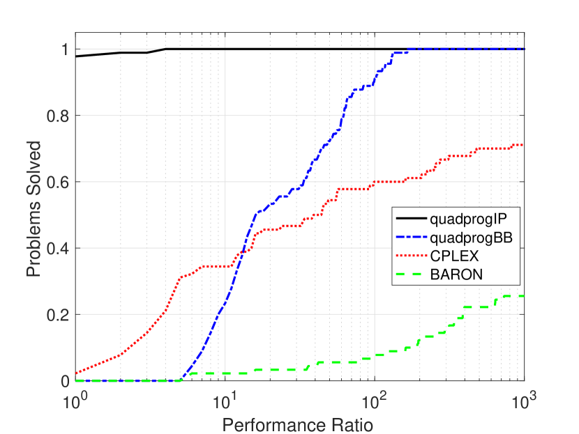
(d) Performance profile for SQP instances.  

Figure 1: Solution time in seconds of SQP instances. Size of squares illustrates size of the instance. A square at the maximum value of an axis represents an instances for which the solver in that axis reached maximum running time without solving it.

Figure 1(a) shows that quadprogIP clearly outperforms quadprogBB by solving all SQP instances in a time that is one to two orders of magnitude faster than quadprogBB   and specially in the larger instances. Similarly, Figure 1(b) shows that quadprogIP clearly outperforms BARON by solving all SQP instances in a time that is one to two orders of magnitude faster than BARON, and specially in the larger instances. Although CPLEX solves two small-scale instances faster than quadprogIP, again, in general quadprogIP outperforms CPLEX by orders of magnitude in terms of solution time (see, Figure 1(c)). As Figures 1(a), 1(b), and 1(c) illustrate, the performance of quadprogIP  against the other solvers improves as the SQP instance becomes larger. The performance profile in Figure 1(d) summarizes the clear advantages of solving the very important class of SQP instances with the proposed quadprogIP solution approach.

3.3.2 Results on SQP30 and SQP50 instances.

As Figure 2 shows, the results on the SQP instances SQP30 and SQP50 from Bonami et al. (2016b) is very similar to the ones presented in Section 3.3.1. As with the set of SQP instances, only CPLEX is able to solve a few instances faster than quadprogIP; however, in general quadprogIP outperforms the other solvers by orders of magnitude in terms of solution time.

(a) quadprogIP vs quadprogBB.  

(b) quadprogIP vs BARON.  

(c) quadprogIP vs CPLEX.  

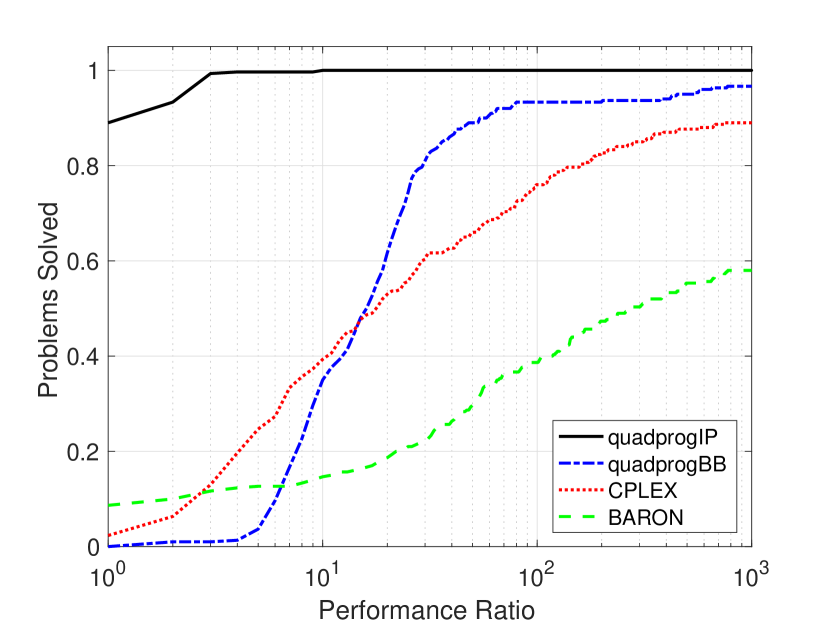
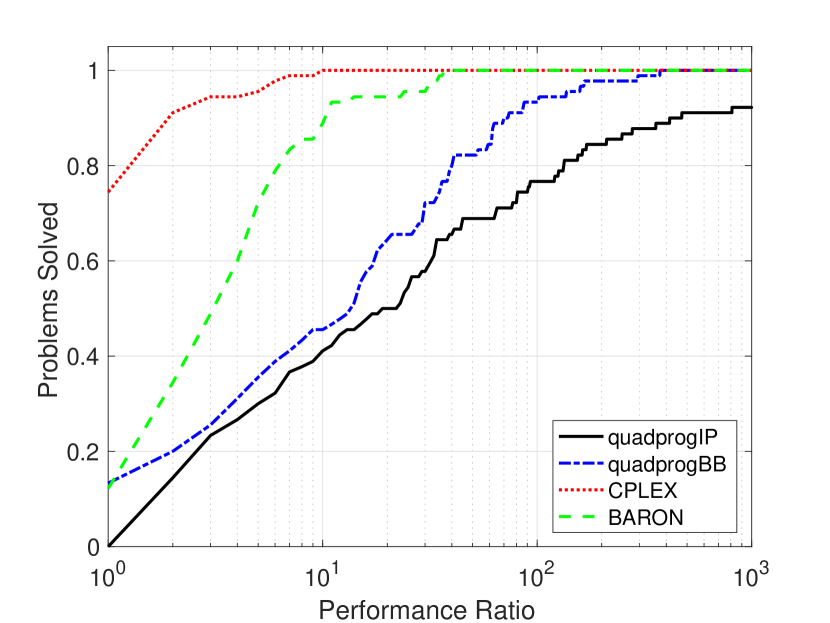
(d) Performance profile for SQP30 and SQP50 instances.  

Figure 2: Solution time in seconds of SQP30 and SQP50 instances. Size of squares illustrates size of the instance. A square at the maximum value of an axis represents an instances for which the solver in that axis reached maximum running time without solving it.

3.3.3 Results on StableQP instances.

In line with the performance of quadprogIP  on SQP, SQP30, and SQP50 instances, it is interesting to see in Table 6 that quadprogIP  clearly outperforms quadprogBB, BARON, and CPLEX in the StableQP instances (see, Section 3.1). In fact, while quadprogIP  solves each of the instances in less than a second, quadprogBB, and CPLEX are unable to solve the instances beyond $k\geq 4$ within the maximum allowed solution time of $10^{4}$ seconds, while BARON is unable to solve the instances beyond $k\geq 3$ within the maximum allowed solution time.

	Solution Time (s.)
$k$	quadprogIP	quadprogBB	B͡ARON	C͡PLEX
1	0.34	3.67	8.93	0.39
2	0.25	6.28	2573.77	8.75
3	0.34	12.56	-	685.70
4	0.43	-	-	-
5	0.49	-	-	-
6	0.51	-	-	-
7	0.46	-	-	-
8	0.49	-	-	-

Table 6: Solution time in seconds for StableQP instances. Dash “-” indicates that the solver was unable to solve the instance within the maximum allowed time.

3.3.4 Results on Scozzari/Tardella instances.

The Scozzari/Tardella from Scozzari and Tardella (2008) are composed of much larger-scale instances of SQP than the ones considered so far. Table 7, as with the previously discussed groups of standard QP instances, clearly shows that quadprogIP is able to solve these instances faster than the other solvers, and is able to solve more large-scale instances than the other solvers.

	Solution Time (s.)
Scozzari/Tardella instance	quadprogIP	quadprogBB	B͡ARON	C͡PLEX
Problem_30x30_0.75.mps.mat:	0.51	5.27	39.32	5.56
Problem_50x50_0.75.mps.mat:	11.78	48.29	-	2,162.13
Problem_100x100_0-1.mps.mat:	1.54	1,412.16	223.54	154.71
Problem_100x100_0.5.mps.mat:	6.71	319.82	-	-
Problem_100x100_0.75.mps.mat:	36.76	1,519.61	-	-
Problem_200x200_0-1.mps.mat:	36.86	-	-	9,995.67
Problem_200x200_0.5.mps.mat:	175.15	-	-	-
Problem_500x500_0-1.mps.mat:	240.09	-	-	-
Problem_500x500_0.25.mps.mat:	2,092.48	-	-	-
Problem_1000x1000_0.25.mps.mat:	-	-	-	-
Problem_Q30.mps.mat:	0.54	4.27	-	-
Problem_Q50.mps.bar.mat:	2.45	8,476.70	-	-
Problem_Q100.mps.bar.mat:	4.71	-	-	-
Problem_Q150.mps.mat:	20.89	-	-	-

Table 7: Solution time in seconds for Scozzari/Tardella instances. Dash “-” indicates that the solver was unable to solve the instance within the maximum allowed time.

3.3.5 Results on BoxQP instances.

In Figure 3, we compare the performance of quadprogIP  on the BoxQP instances against the other three selected solvers. It is clear from Figure 3(a) that while quadprogIP  outperforms quadprogBB in the smaller BoxQP instances (ranging between 20–60 decision variables), quadprogBB outperforms quadprogIP  for larger BoxQP instances (ranging between 60–100 decision variables), where quadprogIP  is typically unable to solve the instance within the $10^{4}$ maximum solution time.

(a) quadprogIP vs quadprogBB.  

(b) quadprogIP vs BARON.  

(c) quadprogIP vs CPLEX.  

(d) Performance profile for BoxQP instances.  

Figure 3: Solution time in seconds of BoxQP instances. Size of squares illustrates size of the instance. A square at the maximum value of an axis represents an instances for which the solver in that axis reached maximum running time without solving it.

Figure 3(b) shows the performance of quadprogIP and BARON on the BoxQP test set. It is clear that BARON outperforms quadprogIP  in most BoxQP instances. Although for instances with less than 40 decision variables the solution time of quadprogIP is not significantly longer than that of BARON. Figure 3(c) shows that CPLEX performs much better than quadprogIP on all BoxQP instances. Figure 3(d) summarizes these results, where it is clear that CPLEX and BARON are the best solvers for these BoxQP instances.

It is worth mentioning that the performance of quadprogIP on BoxQP instances can be improved by adding appropriate valid constraints to the IQP (7) formulation of the BoxQP. This valid constraints can be derived from Hansen et al. (1993, Prop. 1). Specifically, notice that the IQP (7) corresponding to (19) can be written as:

$$\begin{array}[]{rllll}\frac{1}{2}\min&(Hl+f)^{\intercal}x-(u-l)^{\intercal}\mu\\ \operatorname{s.t.}&\begin{bmatrix}H&0\\ 0&0\end{bmatrix}\begin{bmatrix}x\\ s\end{bmatrix}+\begin{bmatrix}f+Hl\\ 0\end{bmatrix}+\begin{bmatrix}I\\ I\end{bmatrix}\mu-\begin{bmatrix}\lambda^{x}\\ \lambda^{s}\end{bmatrix}=0\\ &x+s=u-l\\ &0\leq x_{i}\leq z^{x}_{i}(u_{i}-l_{i})&i=1,\dots,n\\ &0\leq s_{i}\leq z^{s}_{i}(u_{i}-l_{i})&i=1,\dots,n\\ &0\leq\lambda^{x}_{i}\leq(1-z^{x}_{i})V_{i}&i=1,\dots,n\\ &0\leq\lambda^{s}_{i}\leq(1-z^{s}_{i})V_{i}&i=1,\dots,n\\ &z^{x}_{i},z^{s}_{i}\in\{0,1\}&i=1,\dots,n.\end{array}$$ (35)

Then, from Hansen et al. (1993, Prop. 1), and Proposition 4 below, it follows that the constraints

$$z^{x}_{i}+z^{s}_{i}=1,\text{for all $i\in\{1,\dots,n\}$ such that $H_{ii}<0$,}$$ (36)

are valid constraints for the optimal solutions of (35). When added to (35), the valid constraints (36) improve the solution time of the approach proposed here to globally solve BoxQP problems.

Proposition 4.

Let $(x,s,\mu,\lambda^{x},\lambda^{s})\in{\mathbb{R}}^{n}_{+}\times{\mathbb{R}}^{n}_{+}\times{\mathbb{R}}^{2n}\times{\mathbb{R}}^{n}_{+}\times{\mathbb{R}}^{n}_{+}$ be a KKT point of (19). Then $e^{\intercal}\lambda^{x}+e^{\intercal}\lambda^{s}\leq M$, where $M$ is given by (20). That is, every KKT point of (19) satisfies the bounds given by (20).

Proof.

Proof. Let $(x,s,\mu,\lambda^{x},\lambda^{s})$ satisfy the KKT conditions of (19). Then

$$\begin{bmatrix}H&0\\ 0&0\end{bmatrix}\begin{bmatrix}x\\ s\end{bmatrix}+\begin{bmatrix}f+Hl\\ 0\end{bmatrix}+\begin{bmatrix}I\\ I\end{bmatrix}\mu-\begin{bmatrix}\lambda^{x}\\ \lambda^{s}\end{bmatrix}=0$$ (37)

$$x^{\intercal}\lambda^{x}=0,s^{\intercal}\lambda^{s}=0,x+s=U$$ (38)

$$x\geq 0,\lambda^{x}\geq 0,\lambda^{s}\geq 0.$$

where $\mu\in{\mathbb{R}}^{n},\lambda^{x}\in\mathbb{R}^{n}_{+},\lambda^{x}\in\mathbb{R}^{n}_{+}$ are respectively the dual multipliers for the $x+s=u-l$, $x\geq 0$, and $s\geq 0$ constraints in (19). Equation (37) implies that

$$\lambda^{x}-\lambda^{s}=Hx+f+Hl.$$ (39)

Thus, using (38), (39), and the results in Section 2.3.2

$$e^{\intercal}\lambda^{x}+e^{\intercal}\lambda^{s} =e^{\intercal}|\lambda^{x}-\lambda^{s}|=\|Hx+f+Hl\|_{1}\leq\|Hx\|_{1}+\|f+Hl\|_{1}\leq M$$

∎

Although the quadprogIP code does not include the strengthening constraints (36) for BoxQPs, the results illustrated on Figure 4 show how adding the valid constraints (36) improves the solution time on a set of spar BoxQP instances ranging on size between 20-40 variables with density between 30-100. In particular, with the addition of these constraints, quadprogIP outperforms quadprogBB on these instances.

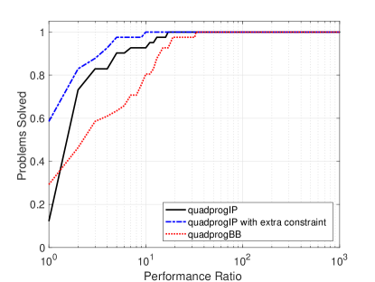
Figure 4: Performance profile for spar BoxQP instances anging on size between 20-40 variables with density between 30-100. Extra constraints refer to adding constraints (36) in the quadprogIP solver.  

Results on CUTEr, Globallib, and RandQP instances.

In Figures 5, we compare the performance of quadprogIP  on the CUTEr, Globallib, and RandQP instances against the other solvers. As Figure 5(a) illustrates, except for a few instances, quadprogIP  has shorter solution times than quadprogBB on the more general CUTEr, Globallib, and RandQP instances of QP. Moreover, quadprogIP  typically solves these problems about 10 times faster than quadprogBB. For these CUTEr, Globallib, and RandQP we find nine (9) instances that are successfully solved by quadprogIP  but not by quadprogBB within the maximum allowed solution time of $10^{4}$ seconds.

As for BARON, it can be seen from Figures 5(b) that quadprogIP is faster on most of the CUTEr, Globallib, and RandQP instances, with quadprogIP being able to solve a fair number of instances that BARON is not able to solve within the maximum allowed time of $10^{4}$ seconds. On the other hand, CPLEX is able to solve most of the CUTEr, Globallib, and RandQP instances faster than quadprogIP; however, still a number of instances are solved faster than CPLEX, and most instances are solved by quadprogIP in a time no larger than 10 times the solution time of CPLEX. Figure 5(d) summarizes these results.

(a) quadprogIP vs quadprogBB.  

(b) quadprogIP vs BARON.  

(c) quadprogIP vs CPLEX.  

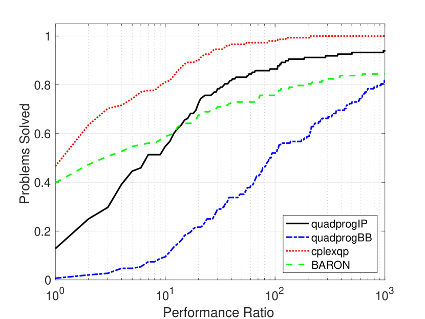
(d) Performance profile for CUTEr, Globallib, and RandQP instances.  

Figure 5: Solution time in seconds of CUTEr, Globallib, and RandQP instances. Size of squares illustrates size of the instance. A square at the maximum value of an axis represents an instances for which the solver in that axis reached maximum running time without solving it.

4 Conclusion

In this paper, we present a new simple and effective approach for the global solution of (non-convex) linearly constrained quadratic problems (QP) by combining the use of the problem’s necessary KKT conditions together with state-of-the-art integer programming solvers. This is done via a reformulation of the QP as a mixed-integer linear program (MILP). We show that in general, this MILP reformulation can be obtained for QPs with a bounded primal feasible set via fundamental results related to the solution of perturbed linear systems of equations (see, e.g., Güler et al. 1995). In practice, quadprogIP is shown to typically outperform by orders of magnitude quadprogBB, BARON, and CPLEX on standard QPs. For general QPs, quadprogIP outperforms quadprogBB, outperforms BARON in most instances, while CPLEX performs the best on these instances. For box-constrained QPs, quadprogIP has a comparable performance to quadprogBB and BARON in small- to medium-scale instances, but is outperformed by these solvers on large-scale instances, while CPLEX performs the best on box-constrained QP instances. Also, unlike quadprogBB, the solution approach proposed here is able to solve QP instances whose dual feasible set is unbounded. The performance of this methodology on standard QP problems allows for the potential use of this solution approach as a basis for the solution of copositive programs (cf., Dür 2010). Which is an interesting direction of future research work.

The proposed IP formulation of general QPs requires the computation of certain type of Hoffman bound (see, e.g., Hoffman 2003) on the system of linear equations defining the problem’s feasible set. Thus, obtaining general and effectively computable bounds of this type is an interesting open question.

We finish by mentioning that a basic implementation of the proposed solution approach referred as quadprogIP  is publicly available at https://github.com/xiawei918/quadprogIP, together with pointers to the test instances used in the article for the numerical experiments, and the raw data of all the solution times used to construct the figures throughout the article in the PDF file raw data.pdf.

References

- Belotti (2010) Belotti, P. 2010. Couenne: a user’s manual. Tech. rep., Clemson University. Available at http://projects.coin-or.%****␣Article_JOC-2016-09-OA-200_Archive.tex␣Line␣3575␣****org/Couenne/browser/trunk/Couenne/doc/couenne-user-manual.pdf.
- Belotti et al. (2009) Belotti, P., J. Lee, L. Liberti, F. Margot, A. Wachter. 2009. Branching and bounds tightening techiques for non-convex MINLP. Optimization Methods and Software 24 597–634.
- Ben-Tal and Nemirovski (2001) Ben-Tal, A., A. Nemirovski. 2001. Lectures on Modern Convex Optimization: Analysis, Algorithms, and Engineering Applications. MPS-SIAM Series on Optimization, SIAM, Philadelphia, PA.
- Bertsekas (1999) Bertsekas, D. 1999. Nonlinear Programming. Athena Scientific, Belmont, MA.
- Bomze (1998) Bomze, I. M. 1998. On standard quadratic optimization problems. Journal of Global Optimization 13 369–387.
- Bomze et al. (2010) Bomze, I. M., F. Frommlet, M. Locatelli. 2010. Copositivity cuts for improving SDP bounds on the clique number. Mathematical Programming 124 13–32.
- Bonami et al. (2016a) Bonami, P., A. Lodi, J. Schweiger, A. Tramontani. 2016a. Solving standard quadratic programming by cutting planes. Tech. Rep. DS4DM-2016-001, hola. Available at http://cerc-datascience.polymtl.ca/wp-content/uploads/2016/06/Technical-Report_DS4DM-2016-001-1.pdf.
- Bonami et al. (2016b) Bonami, Pierre, Oktay Günlük, Jeff Linderoth. 2016b. Solving box-constrained nonconvex quadratic programs. Optimization Online .
- Bundfuss and Dür (2009) Bundfuss, S., Dür. 2009. An adaptive linear approximation algorithm for copositive programs. SIAM Journal on Optimization 20 30–53.
- Burer (2009) Burer, S. 2009. On the copositive representation of binary and continuous nonconvex quadratic programs. Mathematical Programming 120 479–495.
- Burer (2010) Burer, S. 2010. Optimizing a polyhedral-semidefinite relaxation of completely positive programs. Mathematical Programming Computation 2 1–19.
- Burer and Vandenbussche (2009) Burer, S., D. Vandenbussche. 2009. Globally solving box-constrained non-convex quadratic programs with semidefinite-based finite branch-and-bound. Computational Optimization and Applications 43 181–195.
- Chen and Burer (2012) Chen, J., S. Burer. 2012. Globally solving nonconvex quadratic programming problems via completely positive programming. Mathematical Programming Computation 4 33–52.
- CPLEX (2010) CPLEX, IBM ILOG. 2010. 12.2 user?s manual. ILOG. See ftp://ftp. software. ibm. com/software/websphere/ilog/docs/optimization/cplex/ps_usrmancplex. pdf .
- Dobre and Vera (2015) Dobre, C., J. C. Vera. 2015. Exploiting symmetry in copositive programs via semidefinite hierarchies. Mathematical Programming 151 659–680.
- Dong and Anstreicher (2013) Dong, H. B., K. Anstreicher. 2013. Separating doubly nonnegative and completely positive matrices. Mathematical Programming 137 131–153.
- Dür (2010) Dür, M. 2010. Copositive programming – a survey. M. Diehl, F. Glineur, E. Jarlebring, W. Michiels, eds., Recent Advances in Optimization and its Applications in Engineering. Springer, 3–20.
- Eustaquio et al. (2008) Eustaquio, RODRIGO G, ELIZABETH W Karas, ADEMIR A Ribeiro. 2008. Constraint qualifications for nonlinear programming. Federal University of Parana .
- Floudas and Visweswaran (1990) Floudas, C. A., V. Visweswaran. 1990. A global optimization algorithm (GOP) for certain classes of nonconvex NLPs–I. Theory. Computers and Chemical Engineering 14 1397–1417.
- Gao (2004) Gao, D. Y. 2004. Canonical duality theory and solutions to constrained nonconvex quadratic programming. Journal of Global Optimization 29 377–399.
- Giannessi and Tomasin (1973) Giannessi, F., E. Tomasin. 1973. Nonconvex quadratic programs, linear complementarity problems, and integer linear programs. Lecture Notes in Computer Science, vol. 3. Fifth Conference on Optimization Techniques, Springer, Berlin Heidelberg New York, 437–449.
- Gould et al. (2003) Gould, N. I. M., D. Orban, P.L. Toint. 2003. CUTEr and SifDec: A constrained and unconstrained testing environment, revisited. ACM Transactions on Mathematical Software 29 373–394.
- Güler et al. (1995) Güler, O., A. J. Hoffman, U. G. Rothblum. 1995. Approximations to solutions to systems of linear inequalities. SIAM Journal on Matrix Analysis and Applications 16 688–696.
- Hansen et al. (1993) Hansen, Pierre, Brigitte Jaumard, Michèle Ruiz, Junjie Xiong. 1993. Global minimization of indefinite quadratic functions subject to box constraints. Naval Research Logistics (NRL) 40 373–392.
- Hoffman (2003) Hoffman, Alan J. 2003. On approximate solutions of systems of linear inequalities. Selected Papers Of Alan J Hoffman: With Commentary 174–176.
- Horst et al. (2000) Horst, R., P. M. Pardalos, N.V. Thoai. 2000. Introduction to Global Optimization. 2nd ed. Dortrecht: Kluwer.
- Hu et al. (2012) Hu, J., J. E. Mitchell, J. S. Pang, B. Yu. 2012. On linear programs with linear complementarity constraints. Journal of Global Optimization 53 29–51.
- Kim and Kojima (2001) Kim, S., M. Kojima. 2001. Second order cone programming relaxation of nonconvex quadratic optimization problems. Optimization Methods and Software 15 201–224.
- Kim and Kojima (2003) Kim, S., M. Kojima. 2003. Exact solutions of some nonconvex quadratic optimization problems via SDP and SOCP relaxations. Computational Optimization and Applications 26 143–154.
- Mangasarian (1981) Mangasarian, O. L. 1981. A condition number for linear inequalities and linear programs. Tech. Rep. 2231, MRC Technical Summary Report.
- Misener and Floudas (2013) Misener, Ruth, Christodoulos A Floudas. 2013. Glomiqo: Global mixed-integer quadratic optimizer. Journal of Global Optimization 57 3–50.
- Motzkin and Straus (1965) Motzkin, T. S., E. G. Straus. 1965. Maxima for graphs and a new proof of a theorem of Turán. Canadian Journal of Mathematics 17 533–540.
- Nesterov (1998) Nesterov, Y. 1998. Semidefinite relaxation and nonconvex quadratic optimization. Optimization Methods and Software 9 141–160.
- Pardalos and Vavasis (1991) Pardalos, P. M., S. A. Vavasis. 1991. Quadratic programming with one negative eigenvalue is NP-hard. Journal of Global Optimization 1 15–22.
- Peña et al. (2017) Peña, Javier, Juan C. Vera, Luis F. Zuluaga. 2017. Hoffman bounds and norms of set-valued mappings. Tech. rep., Carnegie Mellon University.
- Renegar (2001) Renegar, J. 2001. A Mathematical View of Interior-Point Methods in Convex Optimization, MPS/SIAM Series on Optimization, vol. 3. SIAM.
- Sahinidis (1996) Sahinidis, N. V. 1996. BARON: a general purpose global optimization software package. Journal of Global Optimization 8 201–205.
- Scozzari and Tardella (2008) Scozzari, Andrea, Fabio Tardella. 2008. A clique algorithm for standard quadratic programming. Discrete Applied Mathematics 156 2439–2448.
- Sherali and Adams (1994) Sherali, H., W. Adams. 1994. A hierarchy of relaxations for mixed-integer zero-one programming problems. Discrete Applied Mathematics 52 83–106.
- Tawarmalani and Sahinidis (2004) Tawarmalani, M., N. V. Sahinidis. 2004. Global optimization of mixed-integer nonlinear programs: A theoretical and computational study. Mathematical Programming 99 563–591.
- Vanderbei and Shanno (1999) Vanderbei, R. J., D. F. Shanno. 1999. An interior-point algorithm for nonconvex nonlinear programming. Computational Optimization and Applications 13 231–252.
- Zheng and Ng (2004) Zheng, X. Y., K. F. Ng. 2004. Hoffman’s least error bounds for systems of linear inequalities. Journal of Global Optimization 30 391–403.