Deep 3D Detector for RGB-D Images
Deep Sliding Shapes: A 3D ConvNets Object Detector for RGB-D Images
Deep Sliding Shapes for 3D Object Detection in RGB-D Images
Deep Sliding Shapes for Amodal 3D Object Detection in RGB-D Images
Abstract
We focus on the task of amodal 3D object detection in RGB-D images, which aims to produce a 3D bounding box of an object in metric form at its full extent. We introduce Deep Sliding Shapes, a 3D ConvNet formulation that takes a 3D volumetric scene from a RGB-D image as input and outputs 3D object bounding boxes. In our approach, we propose the first 3D Region Proposal Network (RPN) to learn objectness from geometric shapes and the first joint Object Recognition Network (ORN) to extract geometric features in 3D and color features in 2D. In particular, we handle objects of various sizes by training an amodal RPN at two different scales and an ORN to regress 3D bounding boxes. Experiments show that our algorithm outperforms the state-of-the-art by 13.8 in mAP and is faster than the original Sliding Shapes. Source code and pre-trained models are available.
1 Introduction
Typical object detection predicts the category of an object along with a 2D bounding box on the image plane for the visible part of the object. While this type of result is useful for some tasks, such as object retrieval, it is rather unsatisfying for doing any further reasoning grounded in the real 3D world. In this paper, we focus on the task of amodal 3D object detection in RGB-D images, which aims to produce an object’s 3D bounding box that gives real-world dimensions at the object’s full extent, regardless of truncation or occlusion. This kind of recognition is much more useful, for instance, in the perception-manipulation loop for robotics applications. But adding a new dimension for prediction significantly enlarges the search space, and makes the task much more challenging.
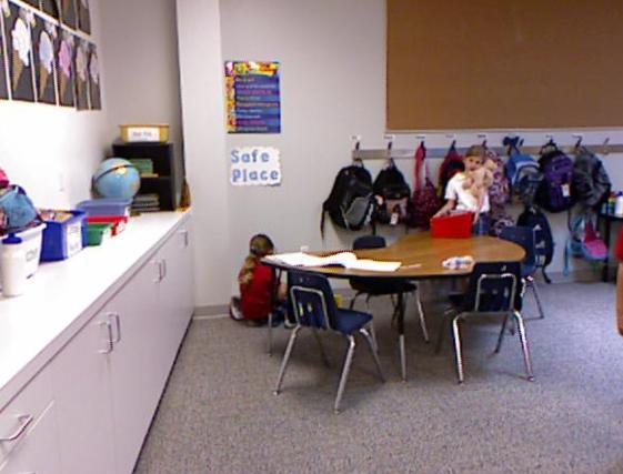
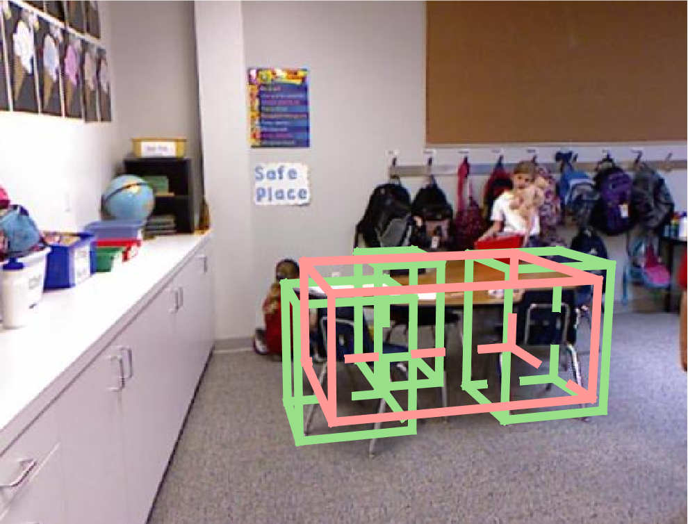
The arrival of reliable and affordable RGB-D sensors (e.g., Microsoft Kinect) has given us an opportunity to revisit this critical task. However naïvely converting 2D detection result to 3D does not work well (see Table 3 and [9]). To make good use of the depth information, Sliding Shapes [23] was proposed to slide a 3D detection window in 3D space. While it is limited by the use of hand-crafted features, this approach naturally formulates the task in 3D. Alternatively, Depth RCNN [9] takes a 2D approach: detect objects in the 2D image plane by treating depth as extra channels of a color image, then fit a 3D model to the points inside the 2D detected window by using ICP alignment. Given existing 2D and 3D approaches to the problem, it is natural to ask: which representation is better for 3D amodal object detection, 2D or 3D? Currently, the 2D-centric Depth RCNN outperforms the 3D-centric Sliding Shapes. But perhaps Depth RCNN’s strength comes from using a well-designed deep network pre-trained with ImageNet, rather than its 2D representation. Is it possible to obtain an elegant but even more powerful 3D formulation by also leveraging deep learning in 3D?
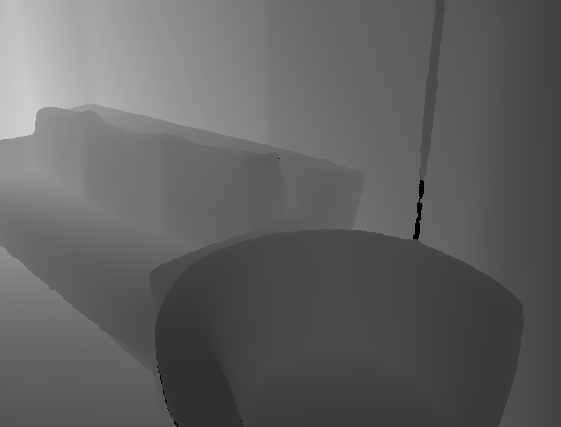
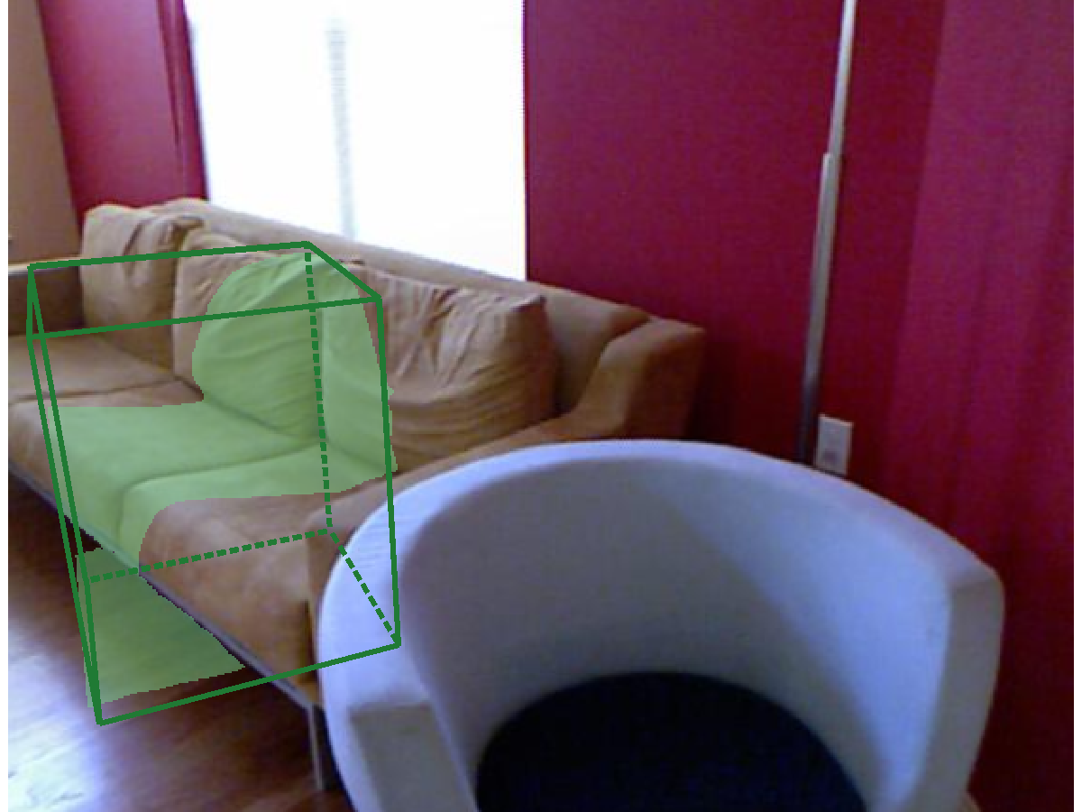
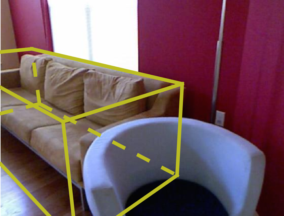
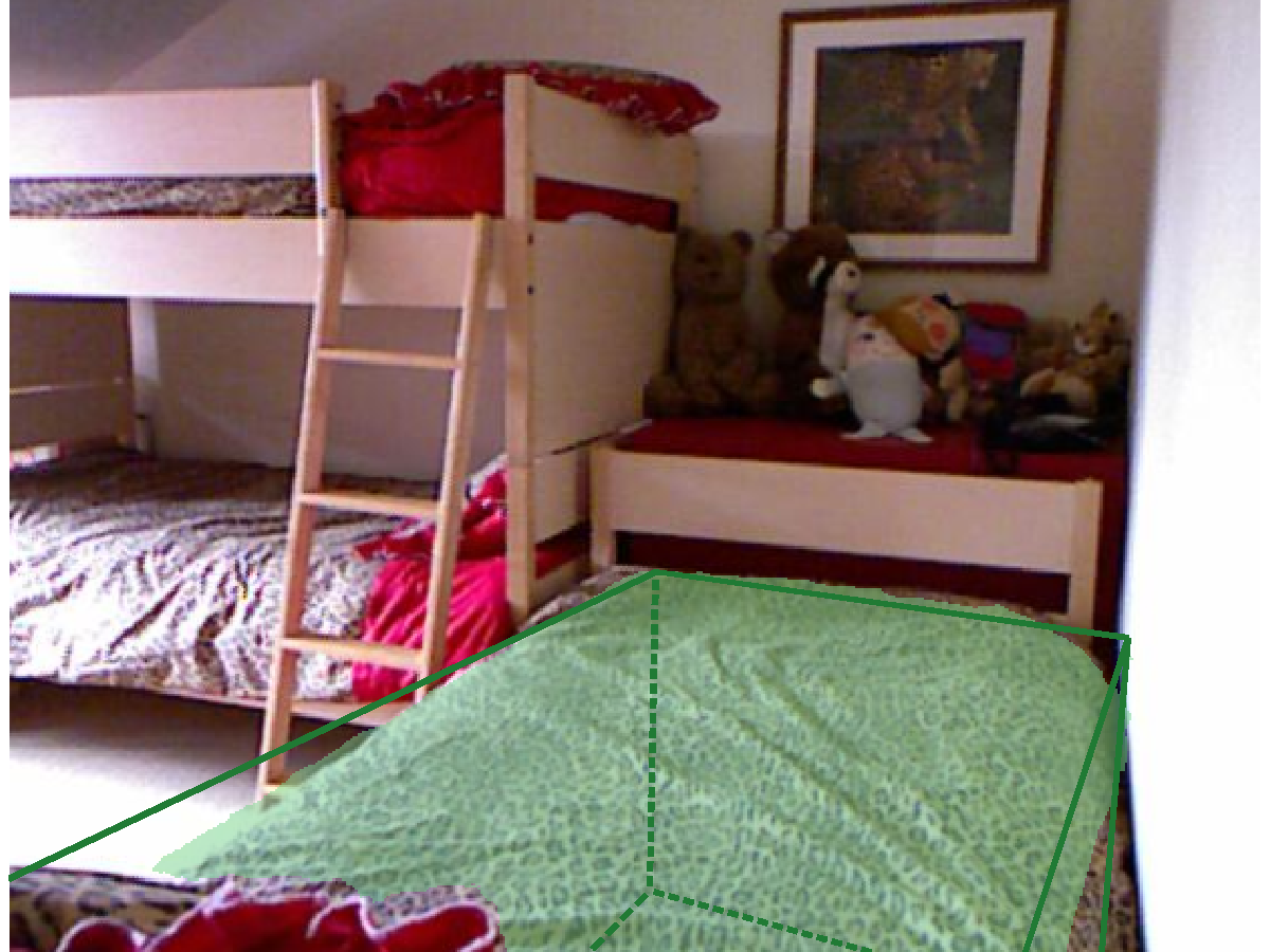
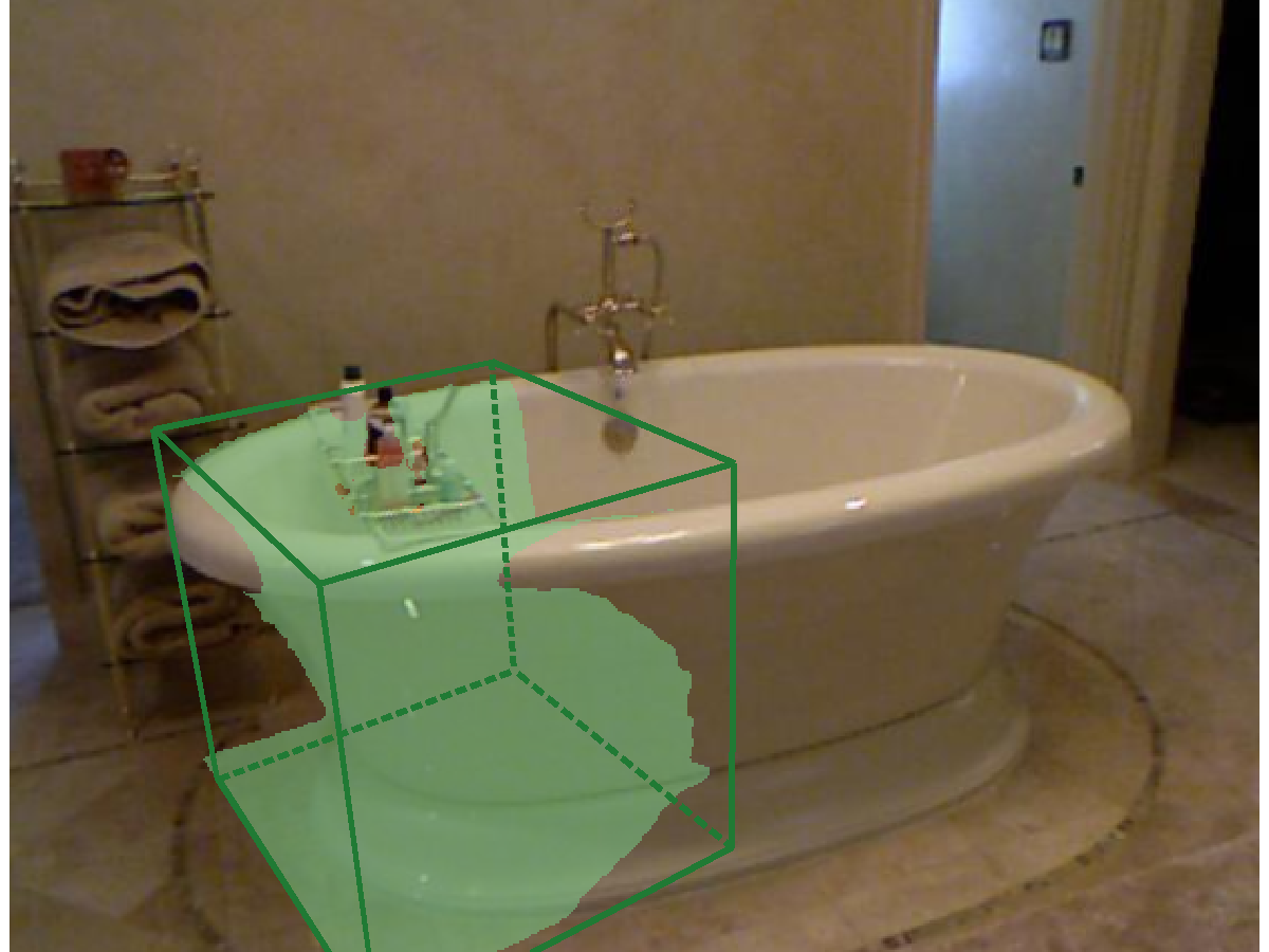
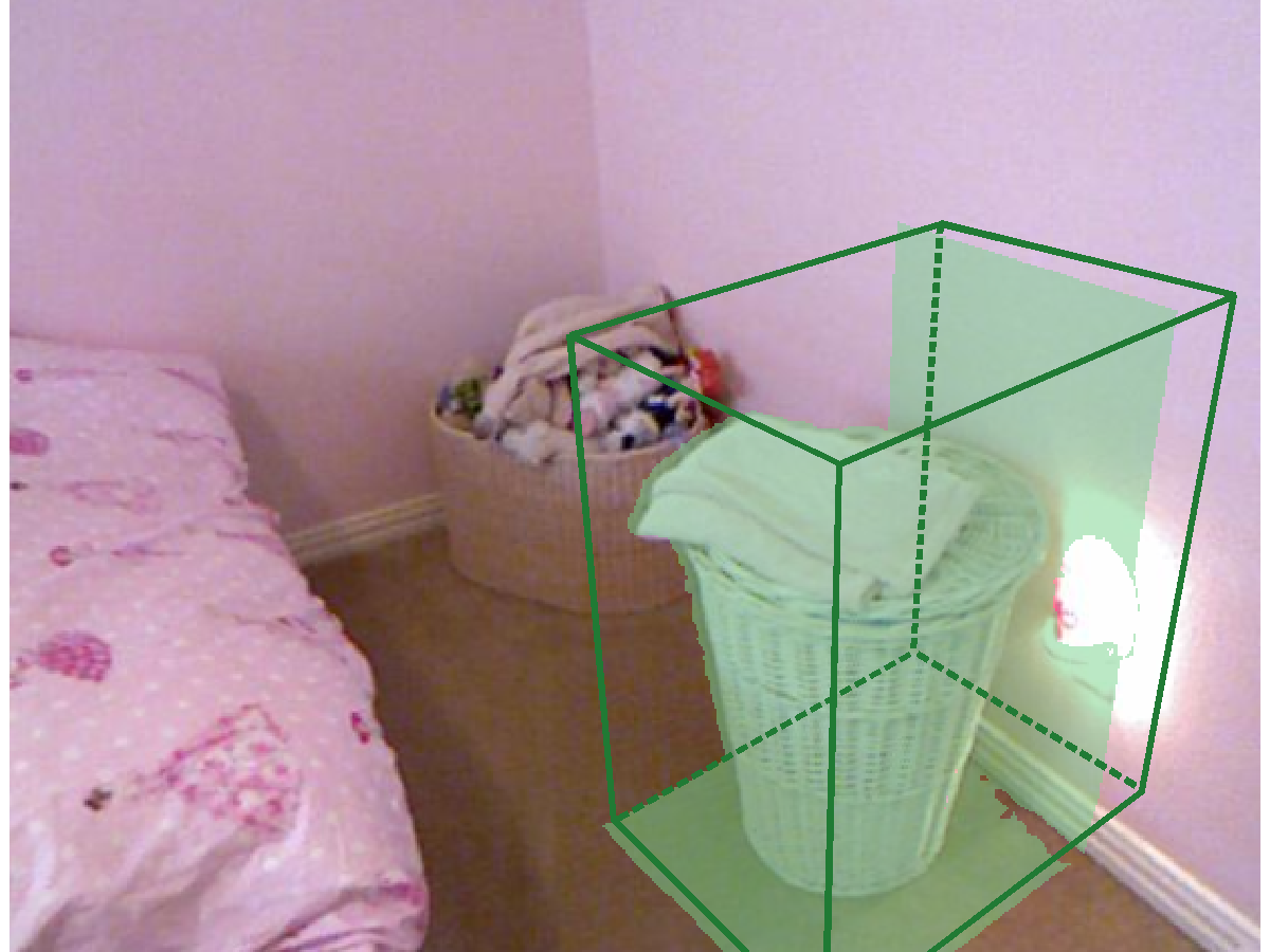
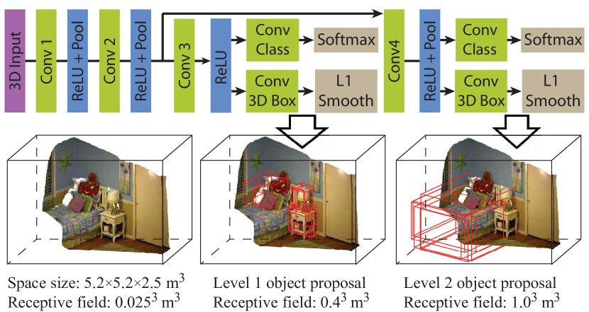
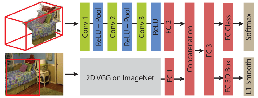
In this paper, we introduce Deep Sliding Shapes, a complete 3D formulation to learn object proposals and classifiers using 3D convolutional neural networks (ConvNets). We propose the first 3D Region Proposal Network (RPN) that takes a 3D volumetric scene as input and outputs 3D object proposals (Figure 1). It is designed to generate amodal proposals for whole objects at two different scales for objects with different sizes. We also propose the first joint Object Recognition Network (PRN) to use a 2D ConvNet to extract image features from color, and a 3D ConvNet to extract geometric features from depth (Figure 2). This network is also the first to regress 3D bounding boxes for objects directly from 3D proposals. Extensive experiments show that our 3D ConvNets can learn a more powerful representation for encoding geometric shapes (Table 3), than 2D representations (e.g. HHA in Depth-RCNN). Our algorithm is also much faster than Depth-RCNN and the the original Sliding Shapes, as it only requires a single forward pass of the ConvNets in GPU at test time.
Our design fully exploits the advantage of 3D. Therefore, our algorithm naturally benefits from the following five aspects: First, we can predict 3D bounding boxes without the extra step of fitting a model from extra CAD data. This elegantly simplifies the pipeline, accelerates the speed, and boosts the performance because the network can directly optimize for the final goal. Second, amodal proposal generation and recognition is very difficult in 2D, because of occlusion, limited field of view, and large size variation due to projection. But in 3D, because objects from the same category typically have similar physical sizes and the distraction from occluders falls outside the window, our 3D sliding-window proposal generation can support amodal detection naturally. Third, by representing shapes in 3D, our ConvNet can have a chance to learn meaningful 3D shape features in a better aligned space. Fourth, in the RPN, the receptive field is naturally represented in real world dimensions, which guides our architecture design. Finally, we can exploit simple 3D context priors by using the Manhattan world assumption to define bounding box orientations.
While the opportunity is encouraging, there are also several unique challenges for 3D object detection. First, a 3D volumetric representation requires much more memory and computation. To address this issue, we propose to separate the 3D Region Proposal Network with a low-res whole scene as input, and the Object Recognition Network with high-res input for each object. Second, 3D physical object bounding boxes vary more in size than 2D pixel-based bounding boxes (due to photography and dataset bias) [15]. To address this issue, we propose a multi-scale Region Proposal Network that predicts proposals with different sizes using different receptive fields. Third, although the geometric shapes from depth are very useful, their signal is usually lower in frequency than the texture signal in color images. To address this issue, we propose a simple but principled way to jointly incorporate color information from the 2D image patch derived by projecting the 3D region proposal.
1.1 Related works
Deep ConvNets have revolutionized 2D image-based object detection. RCNN [7], Fast RCNN [6], and Faster RCNN [17] are three iterations of the most successful state-of-the-art. Beyond predicting only the visible part of an object, [13] further extended RCNN to estimate the amodal box for the whole object. But their result is in 2D and only the height of the object is estimated, while we desire an amodal box in 3D. Inspired by the success from 2D, this paper proposes an integrated 3D detection pipeline to exploit 3D geometric cues using 3D ConvNets for RGB-D images.
2D Object Detector in RGB-D Images
2D object detection approaches for RGB-D images treat depth as extra channel(s) appended to the color images, using hand-crafted features [8], sparse coding [2, 3], or recursive neural networks [22]. Depth-RCNN [10, 9] is the first object detector using deep ConvNets on RGB-D images. They extend the RCNN framework [7] for color-based object detection by encoding the depth map as three extra channels (with Geocentric Encoding: Disparity, Height, and Angle) appended to the color images. [9] extended Depth-RCNN to produce 3D bounding boxes by aligning 3D CAD models to the recognition results. [11] further improved the result by cross model supervision transfer. For 3D CAD model classification, [24] and [19] took a view-based deep learning approach by rendering 3D shapes as 2D image(s).
3D Object Detector
Sliding Shapes [23] is a 3D object detector that runs sliding windows in 3D to directly classify each 3D window. However, because the feature dimension is different per classifier and there are many exemplar classifiers, the algorithm is very slow. Furthermore, the features are hand-crafted and it cannot combine with color features. [29] proposed the Clouds of Oriented Gradients feature on RGB-D images. In this paper we hope to improve these hand-crafted feature representation with 3D ConvNets that can jointly learn powerful 3D and color features from the data.
3D Feature Learning
HMP3D [14] introduced a hierarchical sparse coding technique for unsupervised learning features from RGB-D images and 3D point cloud data. The feature is trained on a synthetic CAD dataset, and test on scene labeling task in RGB-D video. In contrast, we desire a supervised way to learn 3D features using the deep learning techniques that are proved to be more effective for image-based feature learning.
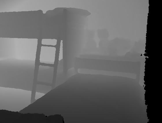
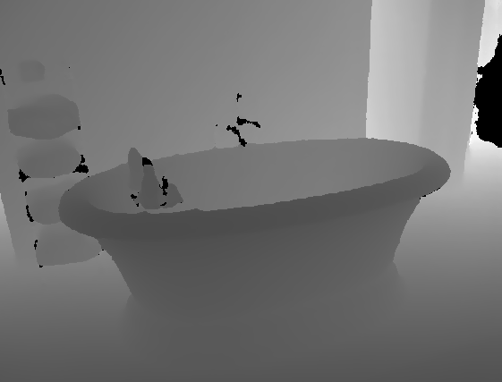
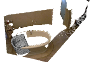
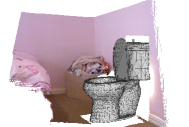
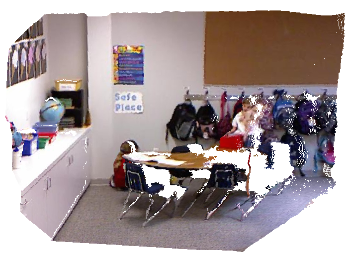
TSDF for a scene used in Region Proposal Network TSDF for six objects used in the Object Recognition Network

3D Deep Learning
3D ShapeNets [27] introduced 3D deep learning for modeling 3D shapes, and demonstrated that powerful 3D features can be learned from a large amount of 3D data. Several recent works [16, 5, 28, 12] also extract deep learning features for retrieval and classification of CAD models. While these works are inspiring, none of them focuses on 3D object detection in RGB-D images.
Region Proposal
For 2D object proposals, previous approaches [25, 1, 10] mostly base on merging segmentation results. Recently, Faster RCNN [17] introduces a more efficient and effective ConvNet-based formulation, which inspires us to learn 3D objectness using ConvNets. For 3D object proposals, [4] introduces a MRF formulation with hand-crafted features for a few object categories in street scenes. We desire to learn 3D features for general scenes from the data using ConvNets.
2 Encoding 3D Representation
The first question that we need to answer for 3D deep learning is: how to encode a 3D space to present to the ConvNets? For color images, naturally the input is a 2D array of pixel color. For depth maps, Depth RCNN [9, 10] proposed to encode depth as a 2D color image with three channels. Although it has the advantage to reuse the pre-trained ConvNets for color images [11], we desire a way to encode the geometric shapes naturally in 3D, preserving spatial locality. Furthermore, compared to methods using hand-crafted 3D features [5, 28], we desire a representation that encodes the 3D geometry as raw as possible, and let ConvNets learn the most discriminative features from the raw data.
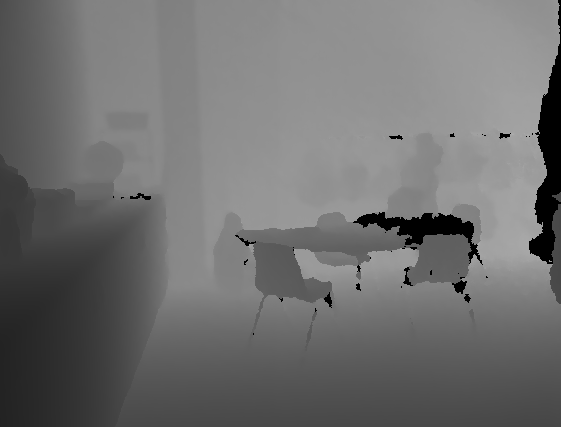
To encode a 3D space for recognition, we propose to adopt a directional Truncated Signed Distance Function (TSDF). Given a 3D space, we divide it into an equally spaced 3D voxel grid. The value in each voxel is defined to be the shortest distance between the voxel center and the surface from the input depth map. Figure 3 shows a few examples. To encode the direction of the surface point, instead of a single distance value, we propose a directional TSDF to store a three-dimensional vector in each voxel to record the distance in three directions to the closest surface point. The value is clipped by , where is the grid size in each dimension. The sign of the value indicates whether the cell is in front of or behind the surface. The conversion from a depth map to a 3D TSDF voxel grid is implemented on a GPU.
To further speed up the TSDF computation, as an approximation, we can also use projective TSDF instead of accurate TSDF where the nearest point is found only on the line of sight from the camera. The projective TSDF is faster to compute, but empirically worse in performance compare to the accurate TSDF for recognition (see Table 2). We also experiment with other encodings, and we find that the proposed directional TSDF outperforms all the other alternatives (see Table 2). Note that we can also encode colors in this 3D volumetric representation, by appending RGB values to each voxel [26].
3 Multi-scale 3D Region Proposal Network
Region proposal generation is a critical step in an object detection pipeline [7, 6, 17]. Instead of exhaustive search in the original Sliding Shapes, we desire a region proposal method in 3D to provide a small set of object agnostic candidates and speed up the computation, and at the same time still utilize the 3D information . But there are several unique challenges in 3D. First, because of an extra dimension, the possible locations for an object increases by 30 times 11145 thousand windows per image in 2D [6] vs. 1.4 million in 3D.. This makes the region proposal step much more important and challenging as it need to be more selective. Second, we are interested in amodal detection that aims to estimate the full 3D box that covers the object at its full extent. Hence an algorithm needs to infer the full box beyond the visible parts. Third, different object categories have very different object size in 3D. In 2D, a picture typically only focuses on the object of interest due to photography bias. Therefore, the pixel areas of object bounding boxes are all in a very limited range [17, 15]. For example, the pixel areas of a bed and a chair can be similar in picture while their 3D physical sizes are very different.
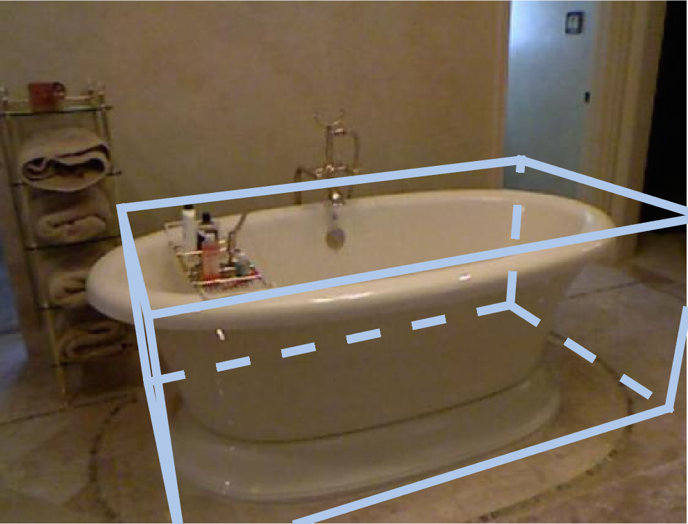
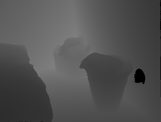
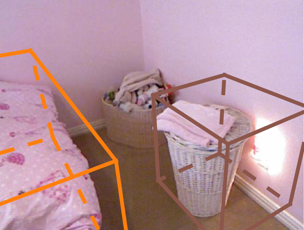
Input: Color and Depth Level 1 Proposals Level 2 Proposals Final Recognition Result

To address these challenges, we propose a multi-scale 3D Region Proposal Network (RPN) to learn 3D objectness using back-propagation (Figure 1). Our RPN takes a 3D scene as input and output a set of 3D amodal object bounding boxes with objectness scores. The network is designed to fully utilize the information from 3D physical world such as object size, physical size of the receptive field, and room orientation. Instead of a bottom-up segmentation based approach (e.g. [25]) that can only identify the visible part, our RPN looks at all the locations for the whole object, in a style similar to sliding windows, to generate amodal object proposals. To handle different object sizes, our RPN targets at two scales with two different sizes of receptive fields.
Range and resolution
For any given 3D scene, we rotate it to align with gravity direction as our camera coordinate system. Based on the specs. for most RGB-D cameras, we target at the effective range of the 3D space meters horizontally, meters vertically, and meters in depth. In this range we encoded the 3D scene by volumetric TSDF with grid size meters, resulting in a volume as the input to the 3D RPN.
Orientation
We desire a small set of proposals to cover all objects with different aspect ratios. Therefore, as a heuristic, we propose to use the major directions of the room for the orientations of all proposals. We use RANSAC plane fitting under the Manhattan world assumption, and use the results as the proposal box orientations. This method can give us pretty accurate bounding box orientations for most object categories. For objects that do not follow the room orientations, such as chairs, their horizontal aspect ratios tend to be a square, and therefore the orientation doesn’t matter much in terms of Intersection-Over-Union (IOU).
Anchor
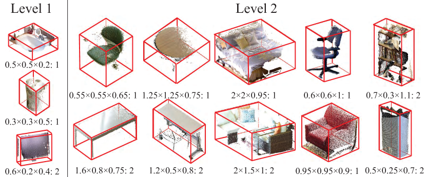
For each sliding window (i.e. convolution) location, the algorithm will predict region proposals. Each of the proposal corresponds to one of the anchor boxes with various sizes and aspect ratios. In our case, based on statistics of object sizes, we define a set of anchors shown in Figure 4. For the anchors with non-square horizontal aspect ratios, we define another anchor with the same size but rotated 90 degrees.
Multi-scale RPN
The physical sizes of anchor boxes vary a lot, from 0.3 meters (e.g. trash bin) to 2 meters (e.g. bed). If we use a single-scale RPN, the network would have to predict all the boxes using the same receptive fields. This means that the effective feature map will contain many distractions for small object proposals. To address this issue, we propose a multi-scale RPN to output proposals at small and big scales, the big one has a pooling layer to increase receptive field for bigger objects. We group the list of anchors into two levels based on how close their physical sizes are to the receptive fields of the output layers, and use different branches of the network to predict them using different receptive fields.
Fully 3D convolutional architecture
To implement a 3D sliding window style search, we choose a fully 3D convolutional architecture. Figure 1 shows our network architecture. The stride for the last convolution layer to predict objectness score and bounding box regression is 1, which is 0.1 meter in 3D. The filter size is for Level 1 and for Level 2, which corresponds to receptive field for Level 1 anchors and for Level 2 anchors.
Empty box removal
Given the range, resolution, and network architecture, the total number of anchors for any image is 1,387,646 (). But on average, of these anchor boxes are almost empty, with point density less than 0.005 points per cm3. To avoid distraction, for both training and testing, we automatically remove these anchors. This is done in constant time, by using 3D integral image. After removing these almost empty boxes, there are on average 107,674 anchors remaining.
Training sampling
For the remaining anchors, we label them as positive if their 3D IOU scores with ground truth are larger than 0.35, and negative if their IOU are smaller than 0.15. In our implementation, each mini-batch contains two images. We randomly sample 256 anchors in each image with positive and negative ratio 1:1. If there are fewer than 128 positive samples we pad the mini-batch with negative samples from the same image. We select them by specifying the weights for each anchor in the final convolution layers. We also try to use all the positives and negatives with proper weighting, but the training cannot converge.
3D box regression
We represent each 3D box by its center and the size of the box in three major directions of the box (the anchor orientation for anchors, and the human annotation for ground truth). To train the 3D box regressor, we will predict the difference of centers and sizes between an anchor box and its ground truth box. For simplicity, we do not do regression on the orientations. For each positive anchor and its corresponding ground truth, we represent the offset of box centers by their difference in the camera coordinate system. For the size difference, we first find the closest matching of major directions between the two boxes, and then calculate the offset of box size in each matched direction. Similarly to [17], we normalize the size difference by its anchor size. Our target for 3D box regression is a 6-element vector for each positive anchor .
Multi-task loss
Following the multi-task loss in [6, 17], for each anchor, our loss function is defined as:
| (1) |
where the first term is for objectness score, and the second term is for the box regression. is the predicted probability of this anchor being an object and is the ground truth (1 if the anchor is positive, and 0 if the anchor is negative). is log loss over two categories (object vs. non object). The second term formulates the 3D bounding box regression for the positive anchors (when ). is smooth loss used for 2D box regression by Fast-RCNN [6].
3D NMS
The RPN network produces an objectness score for each of the non-empty proposal boxes (anchors offset by regression results). To remove redundant proposals, we apply 3D Non-Maximum Suppression (NMS) on these boxes with IOU threshold in 3D, and only pick the top 2000 boxes to input to the object recognition network. These 2000 boxes are only of all sliding windows, and it is one of the key factor that makes our algorithm much faster than the original Sliding Shapes [23].

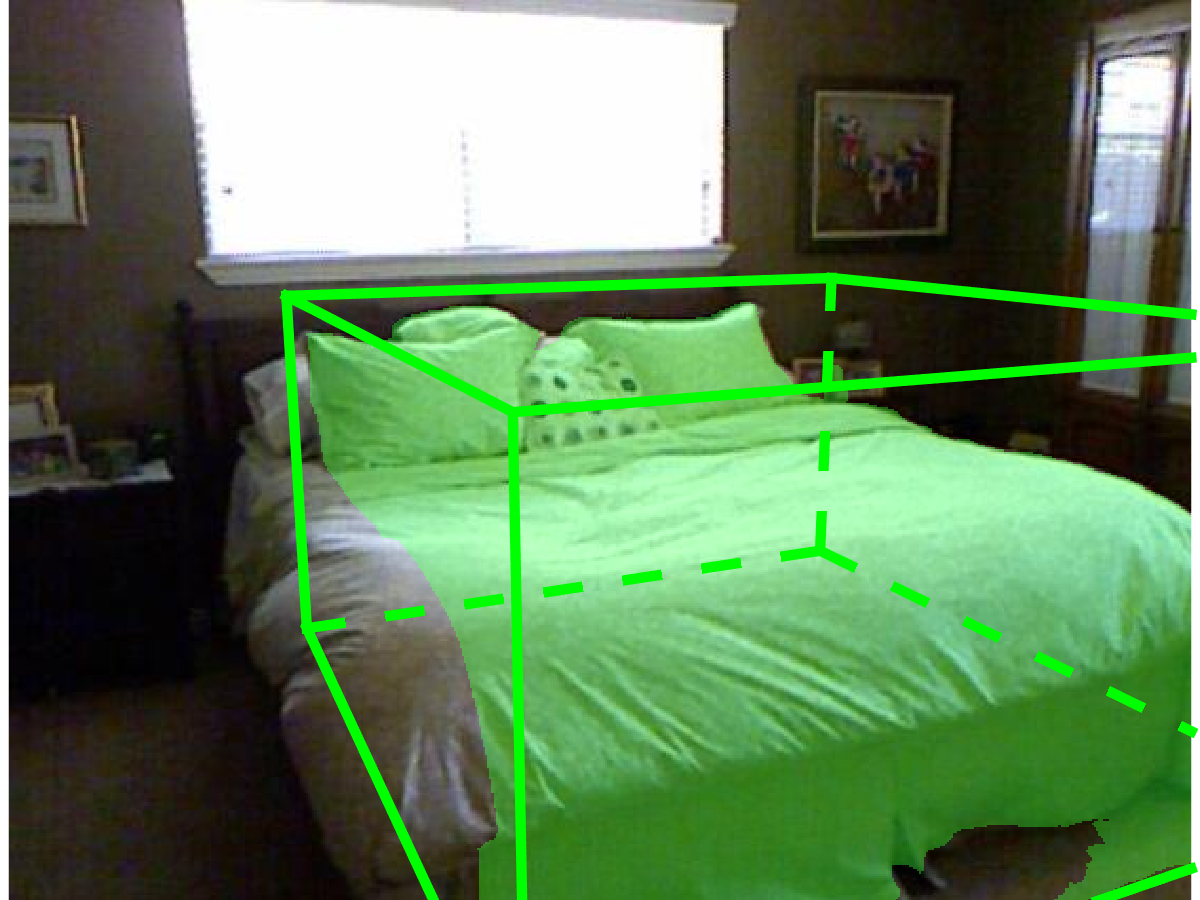
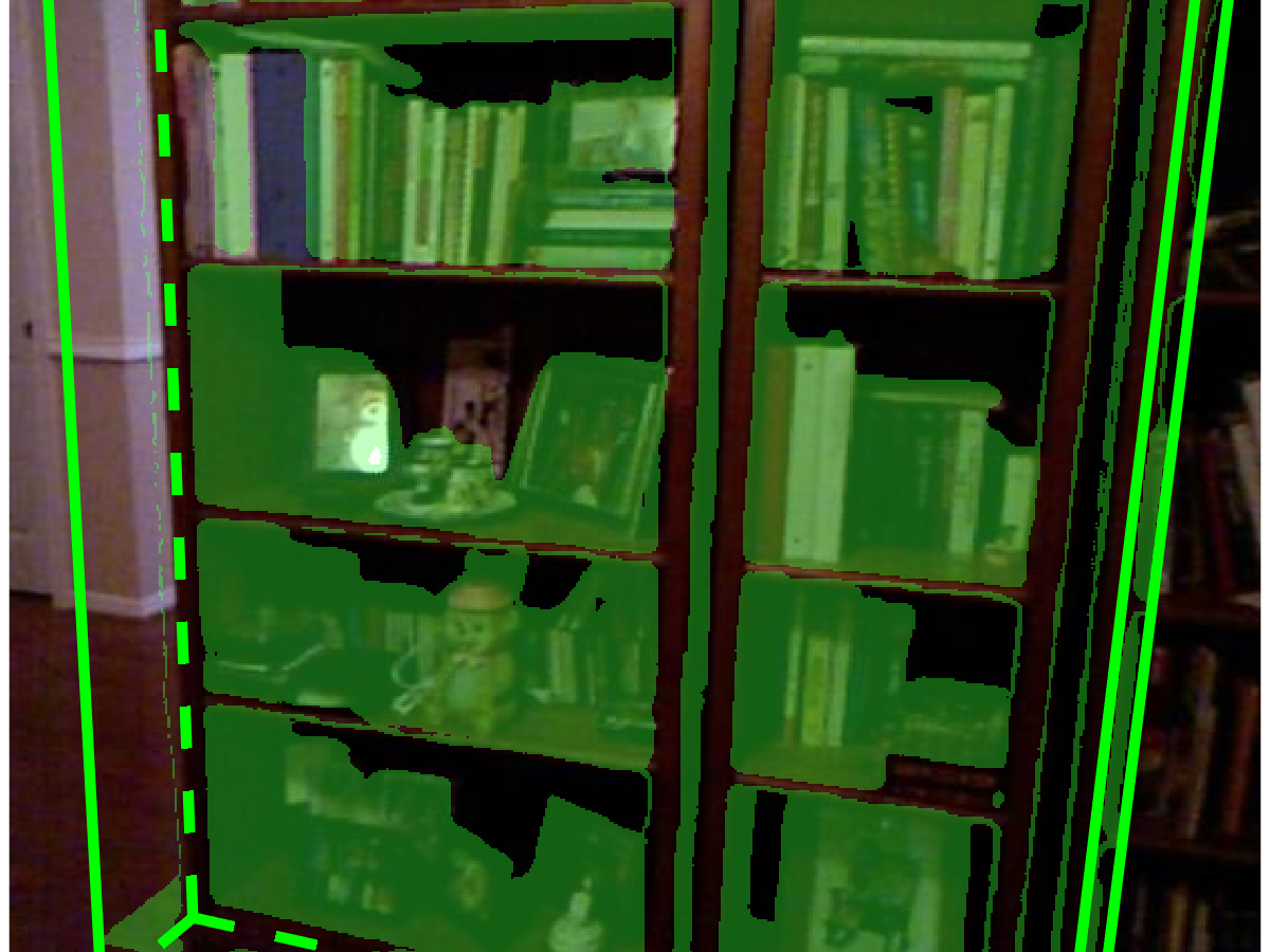
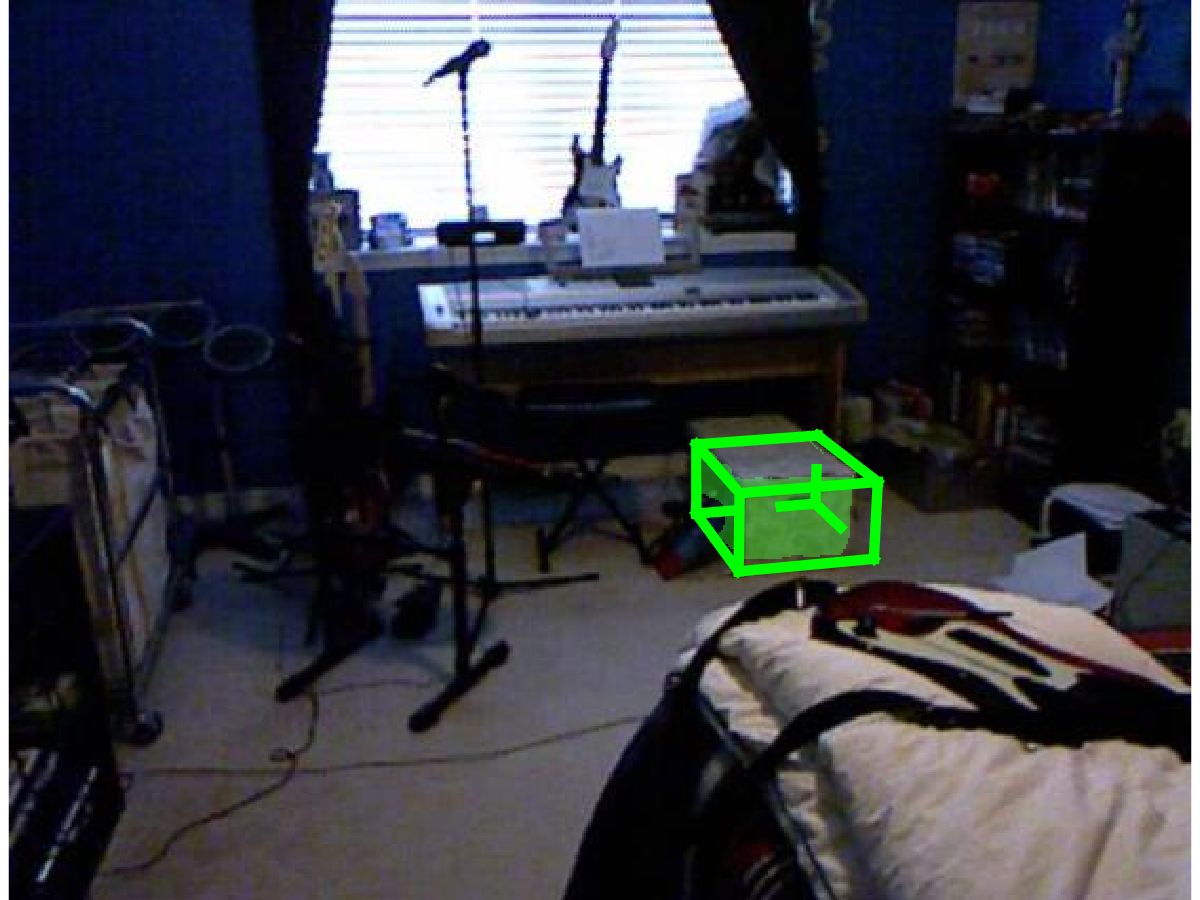
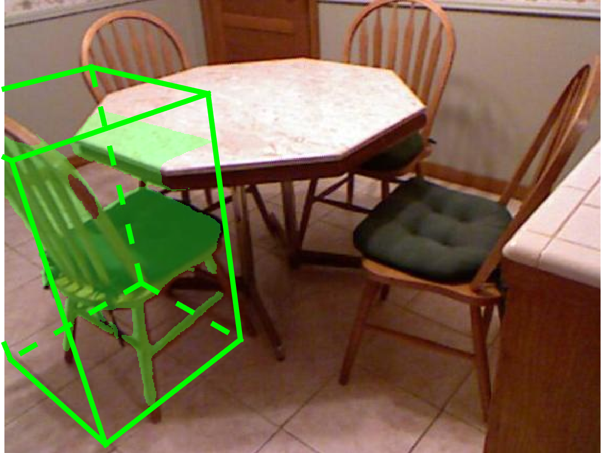
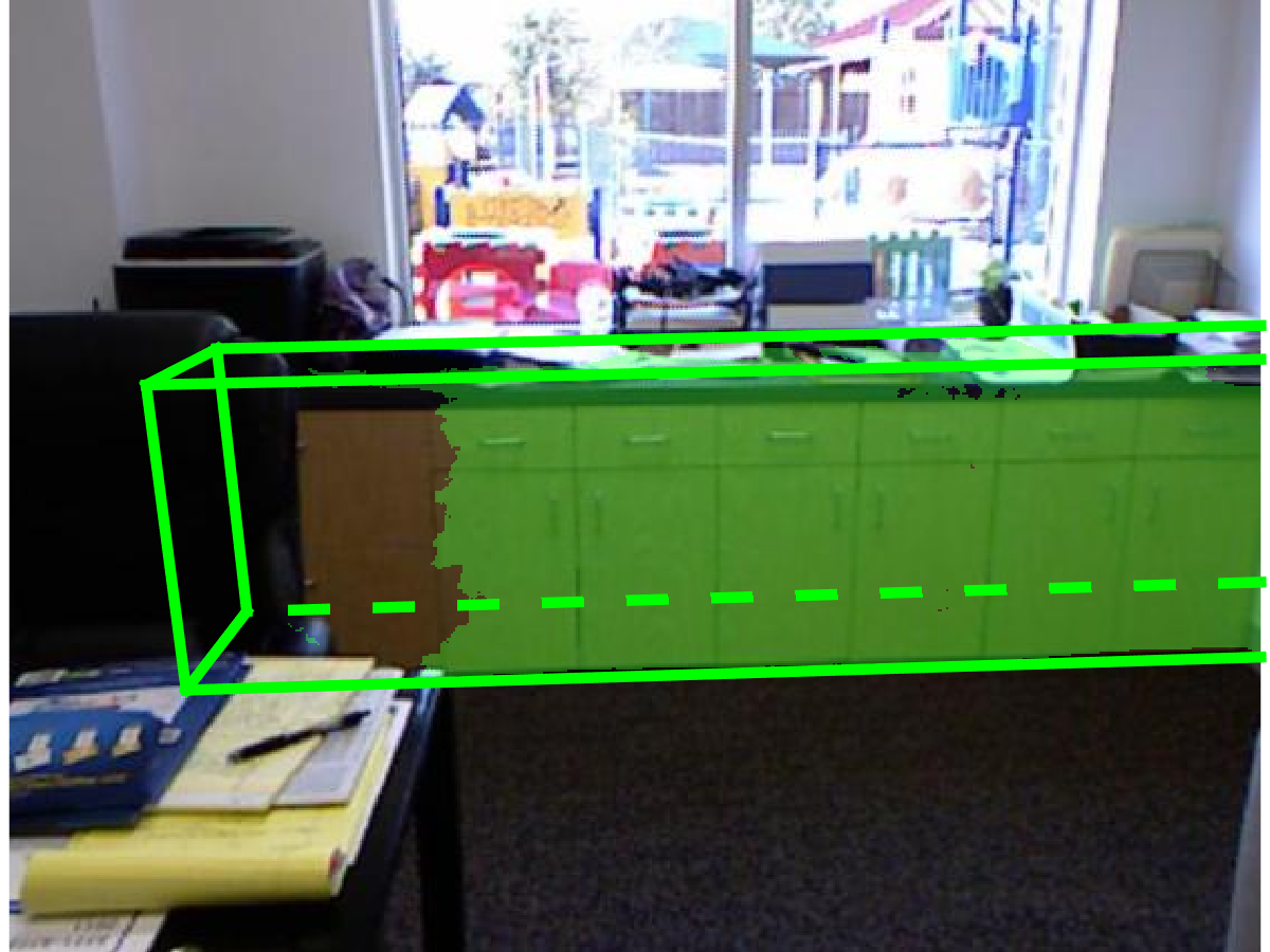
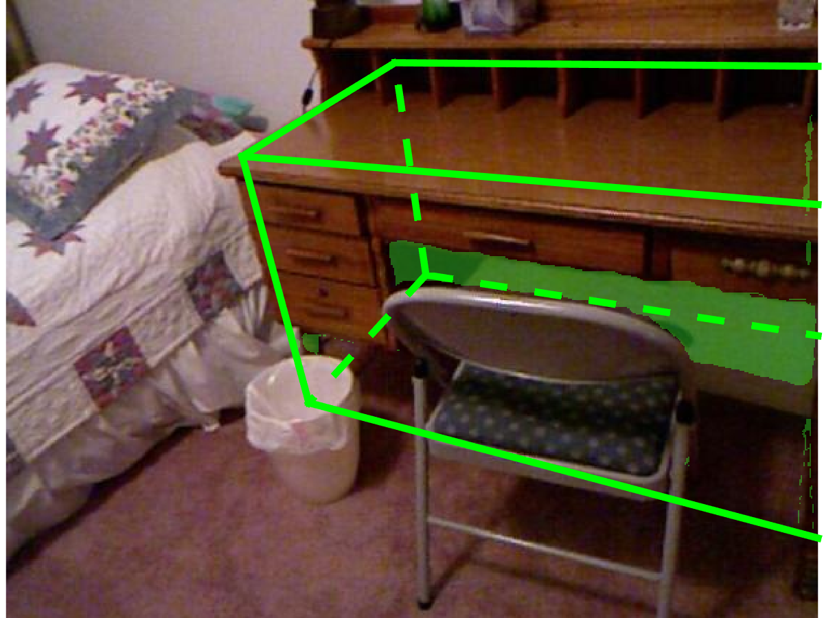
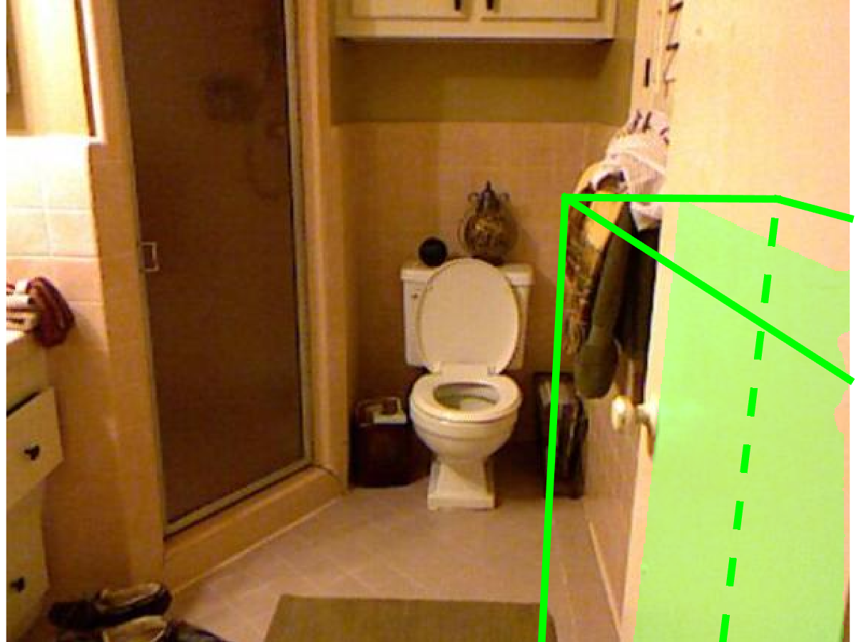
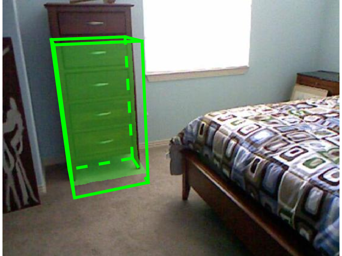
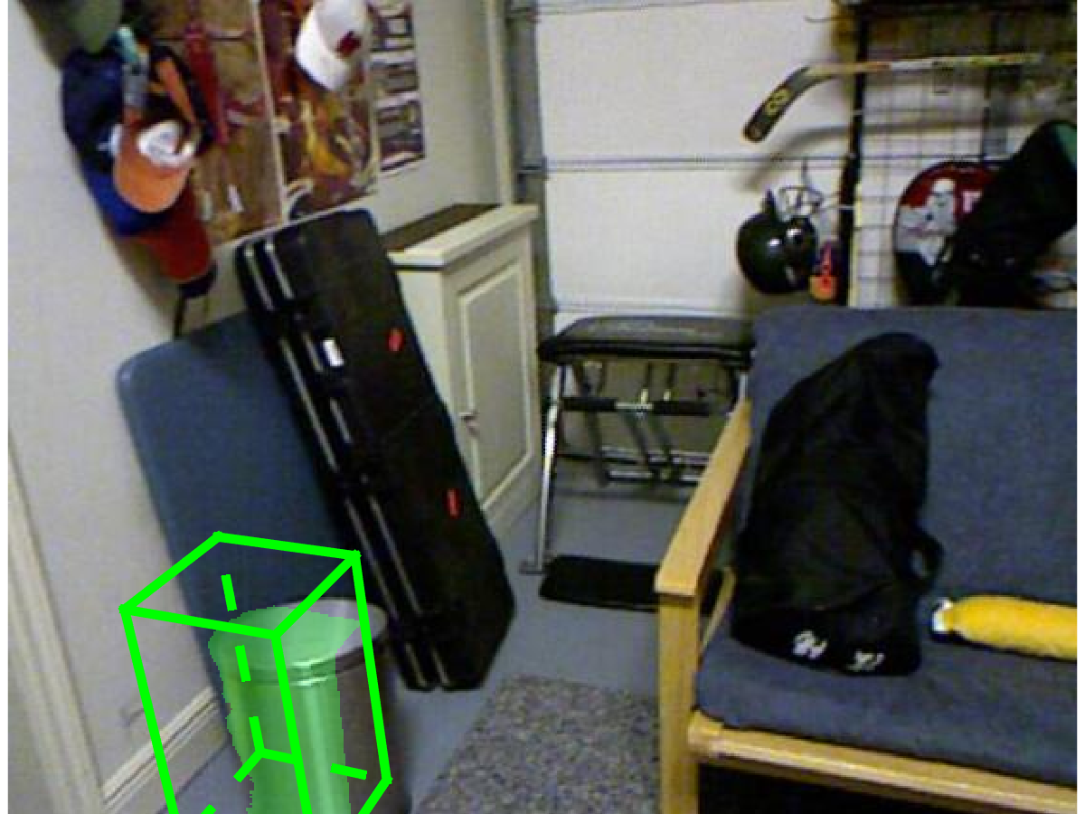
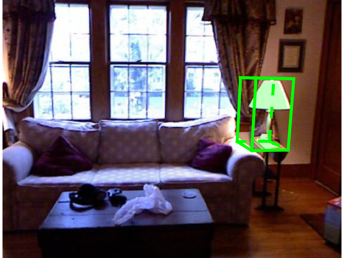
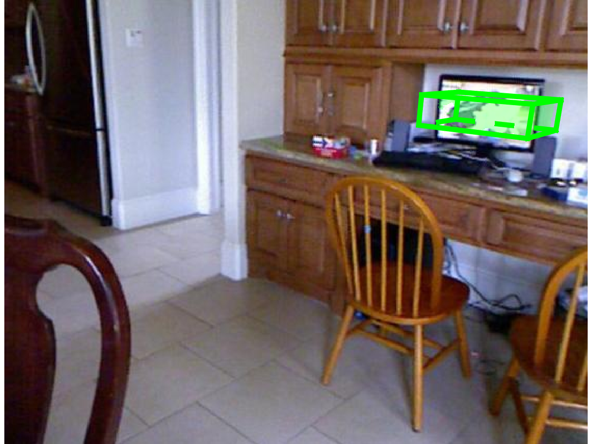
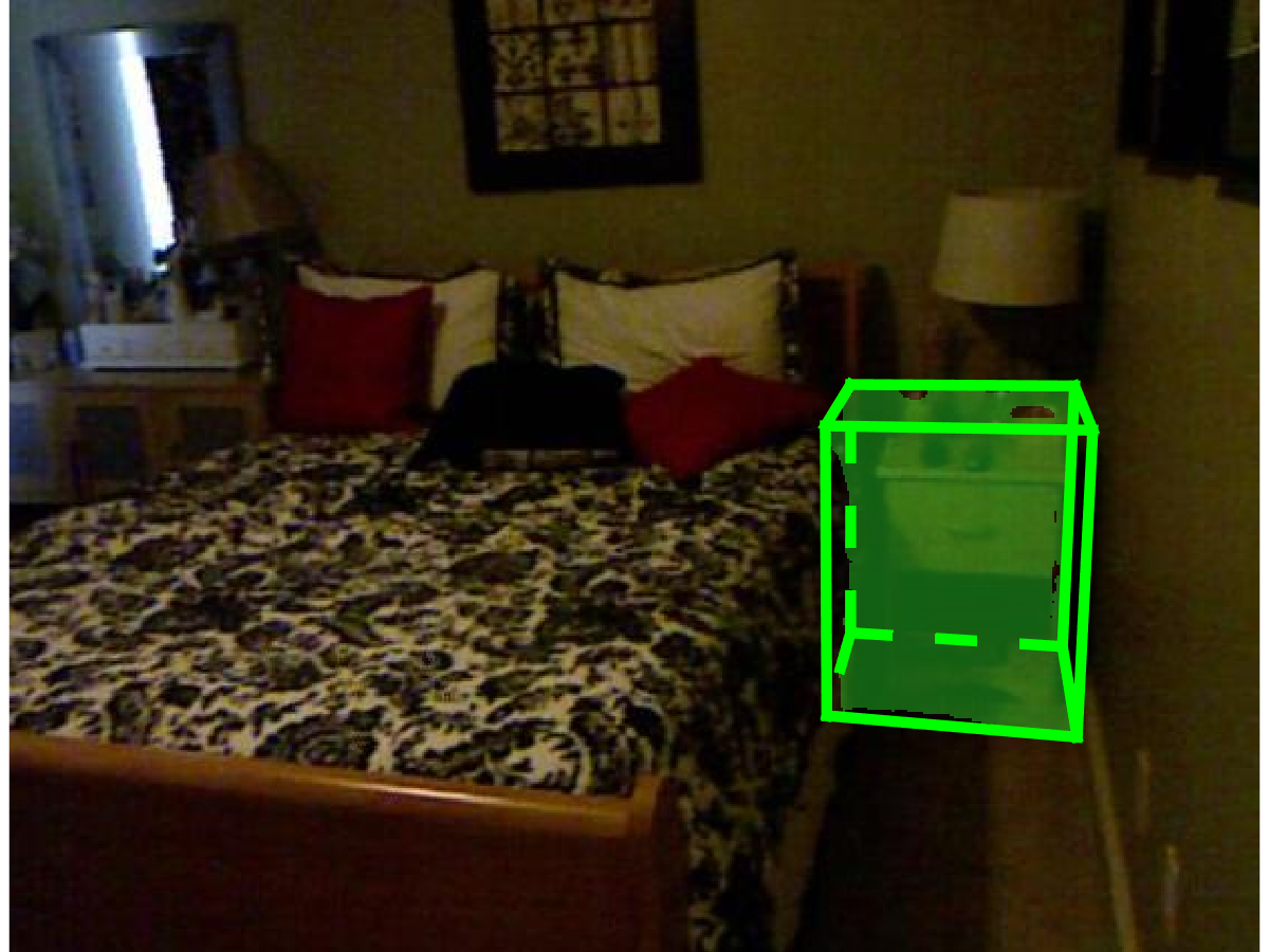
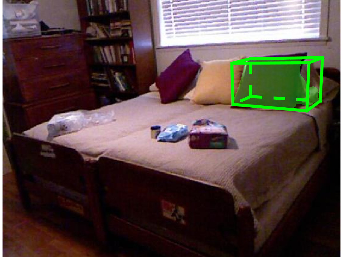
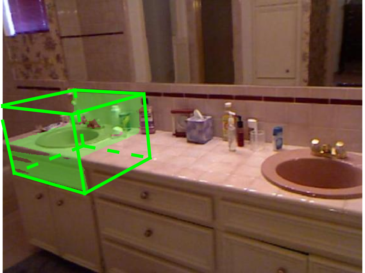
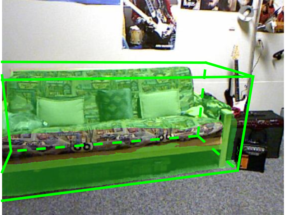
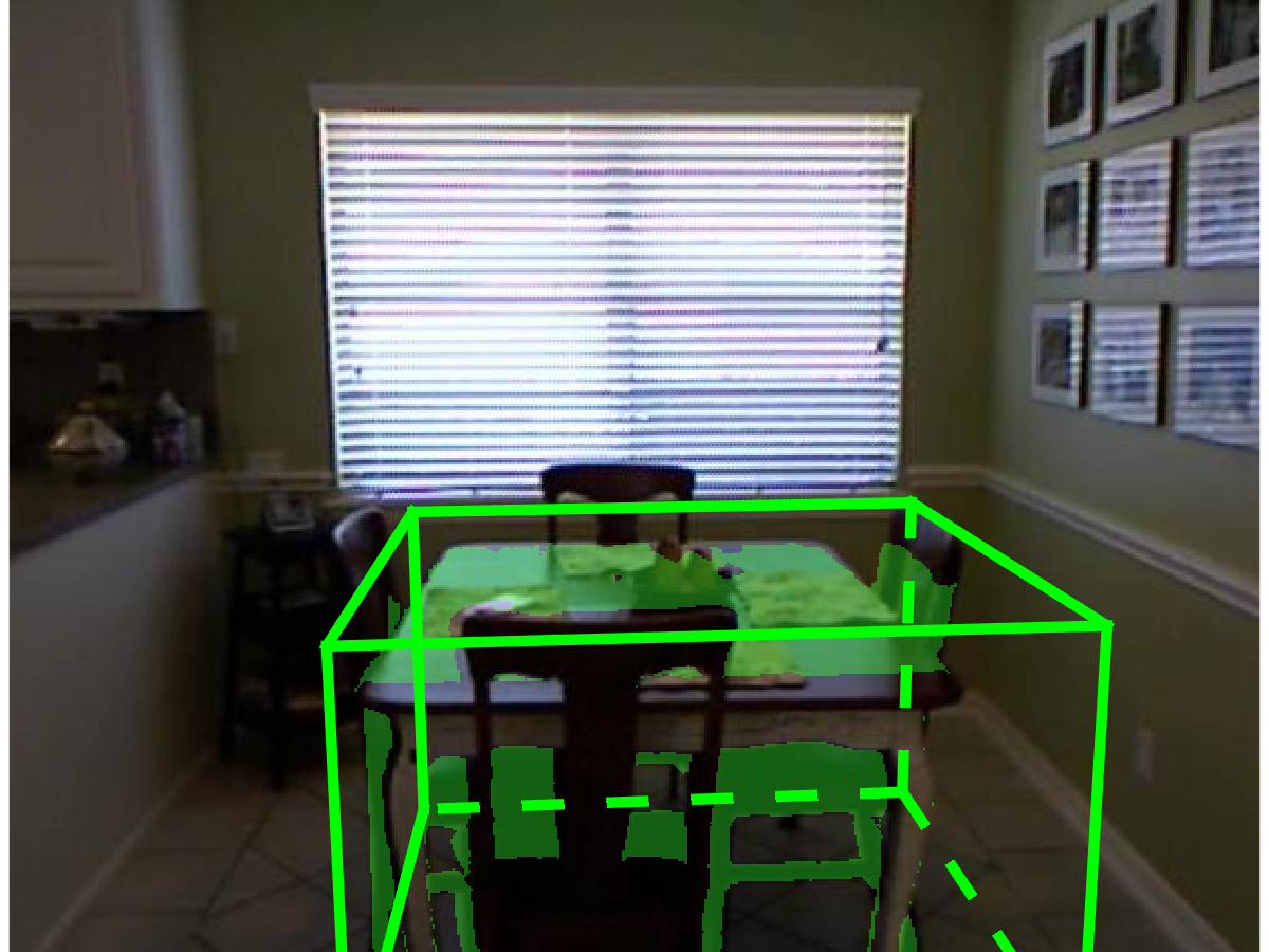
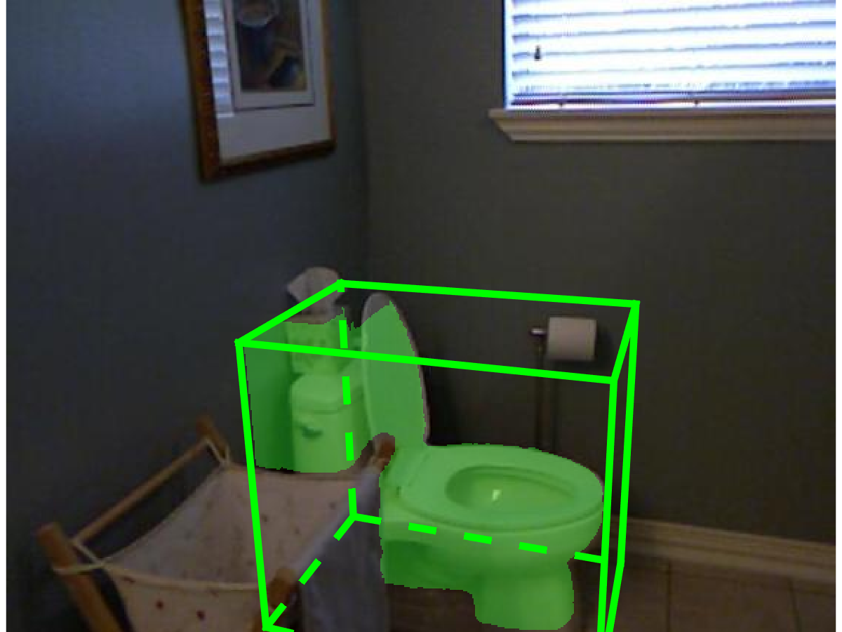
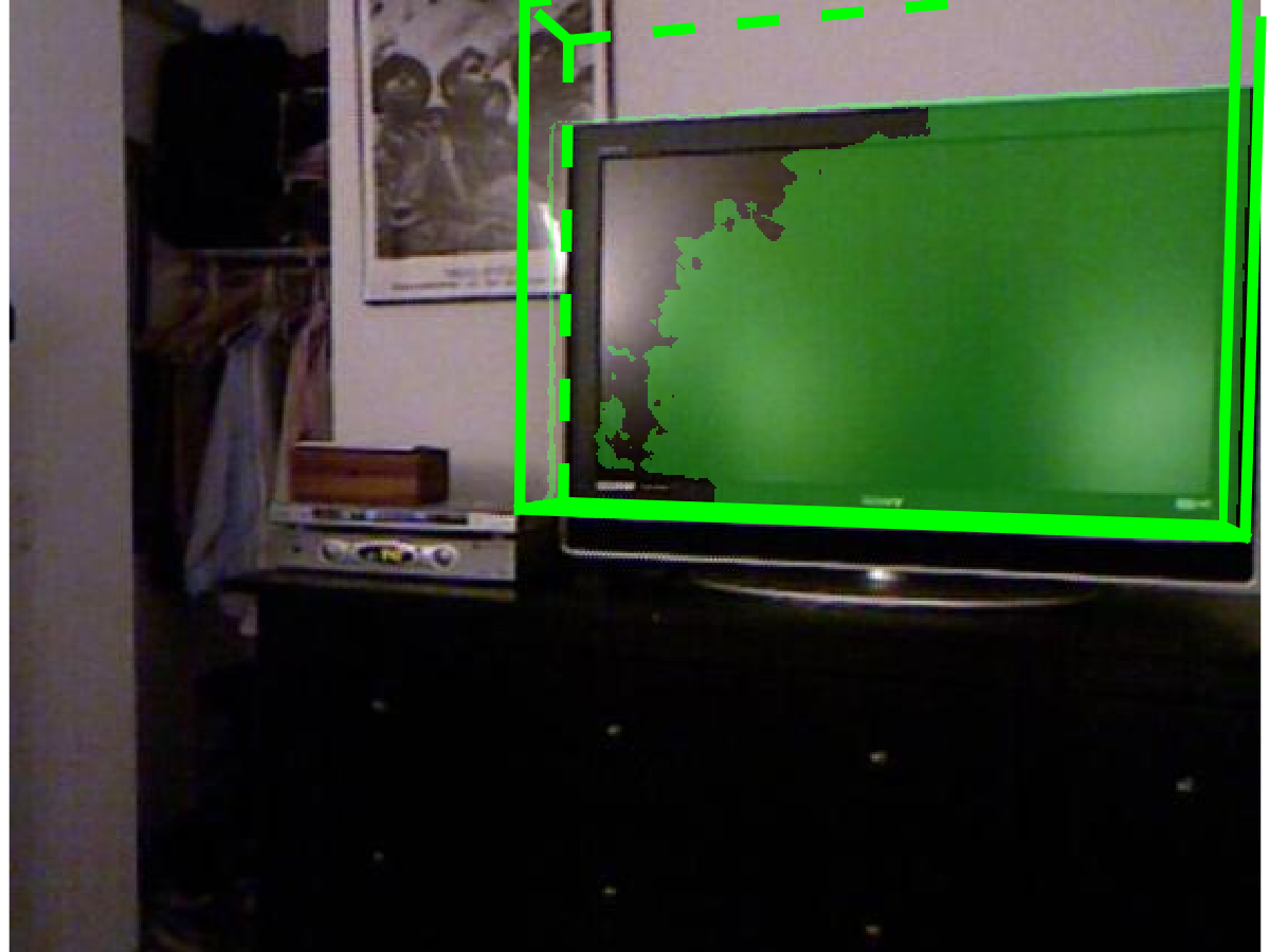


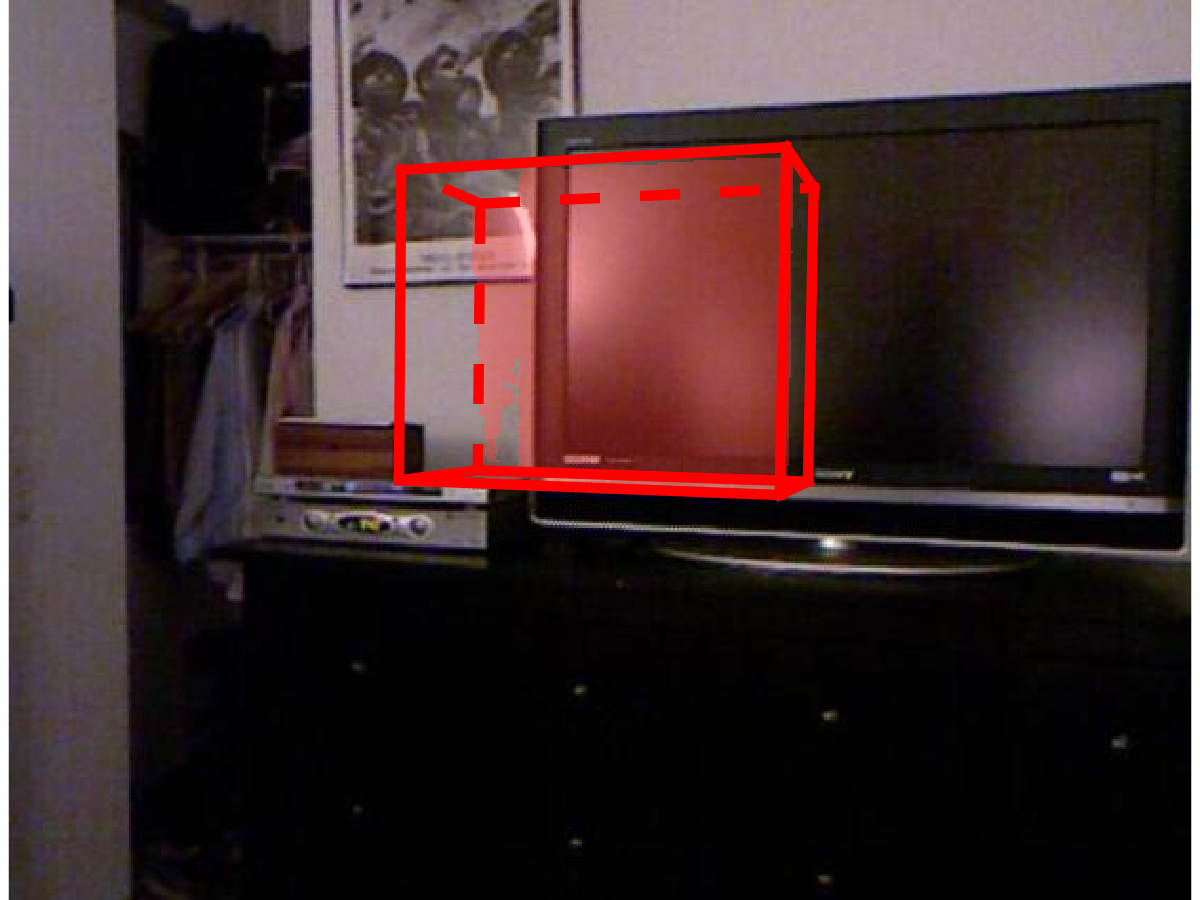
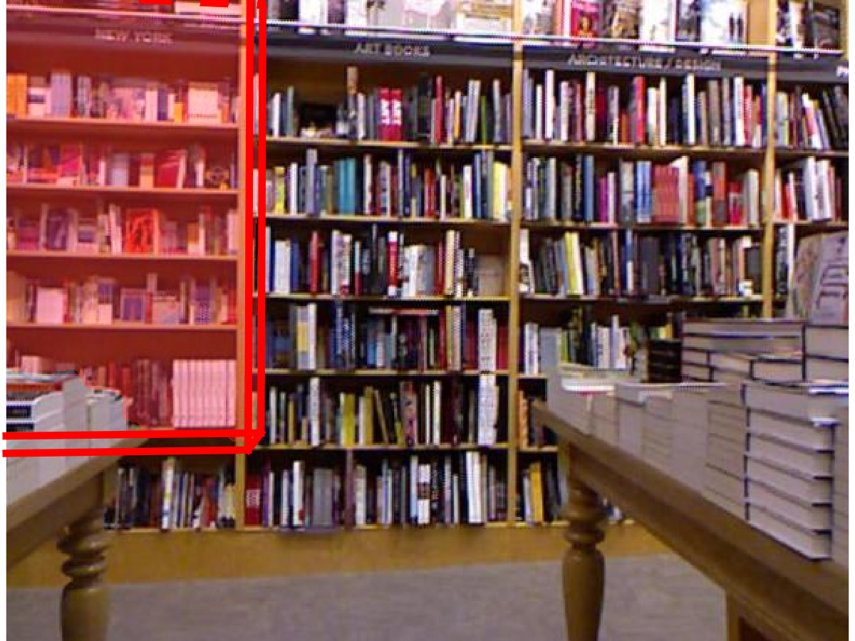
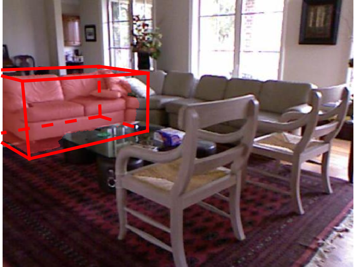
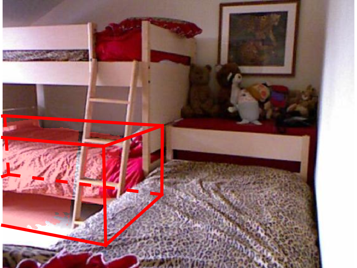
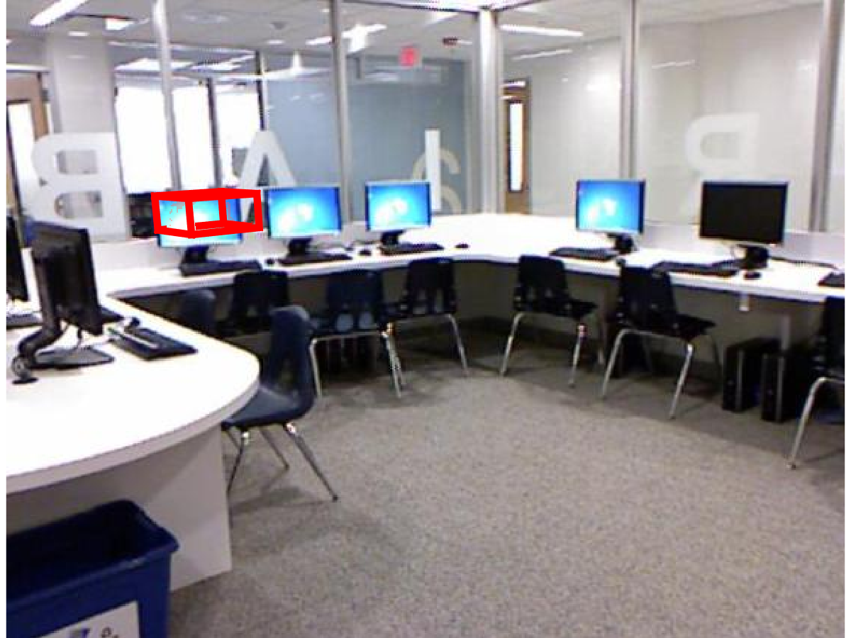
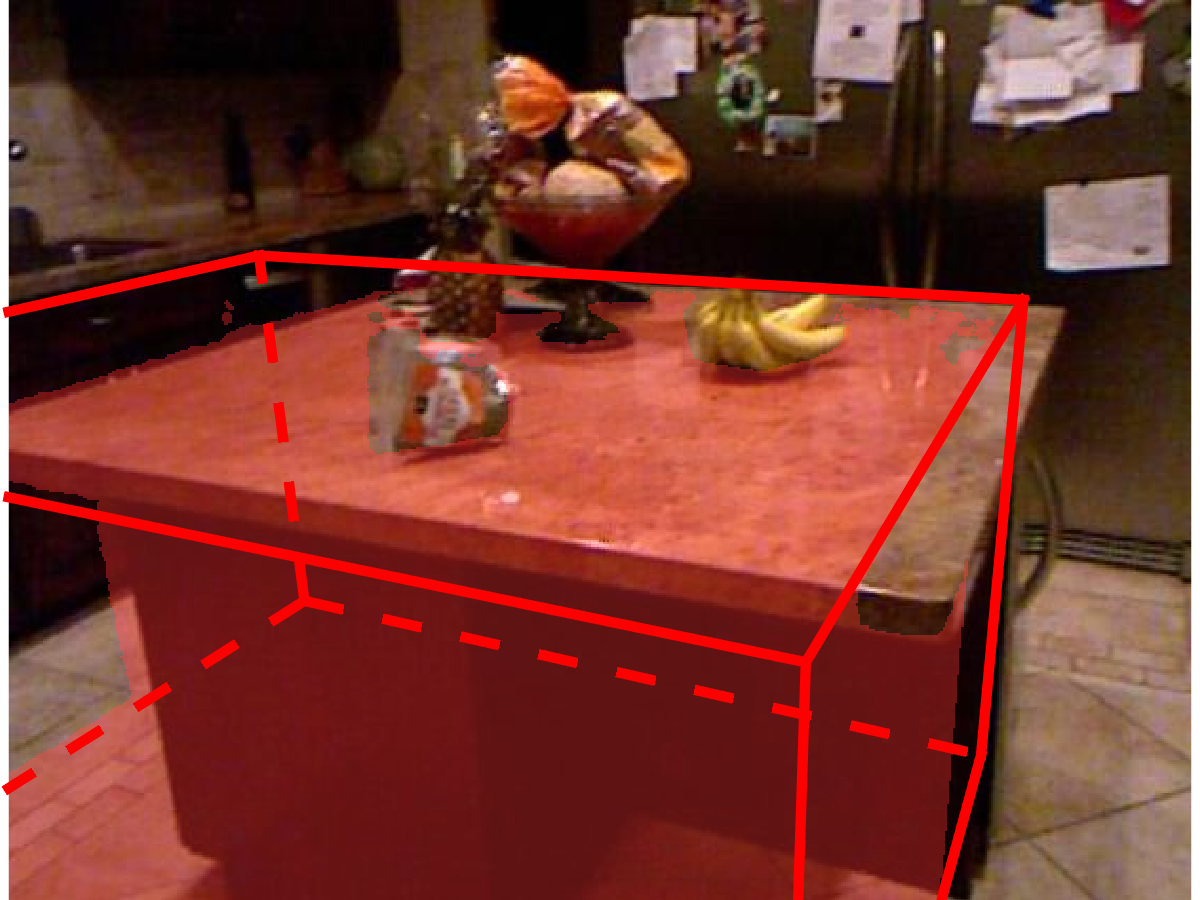
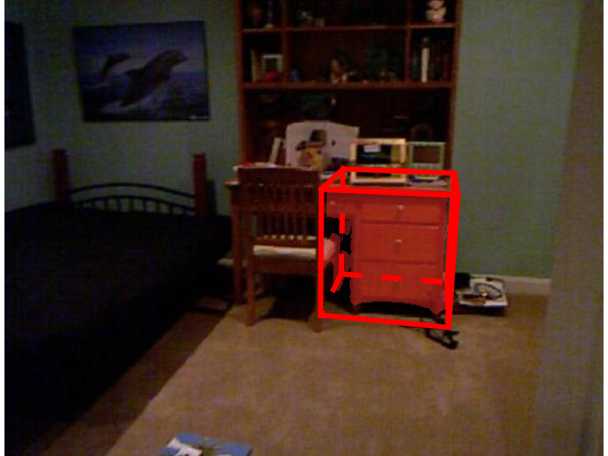
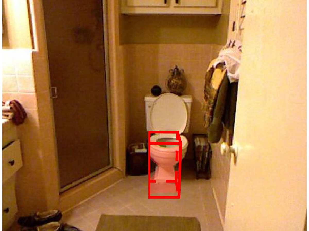
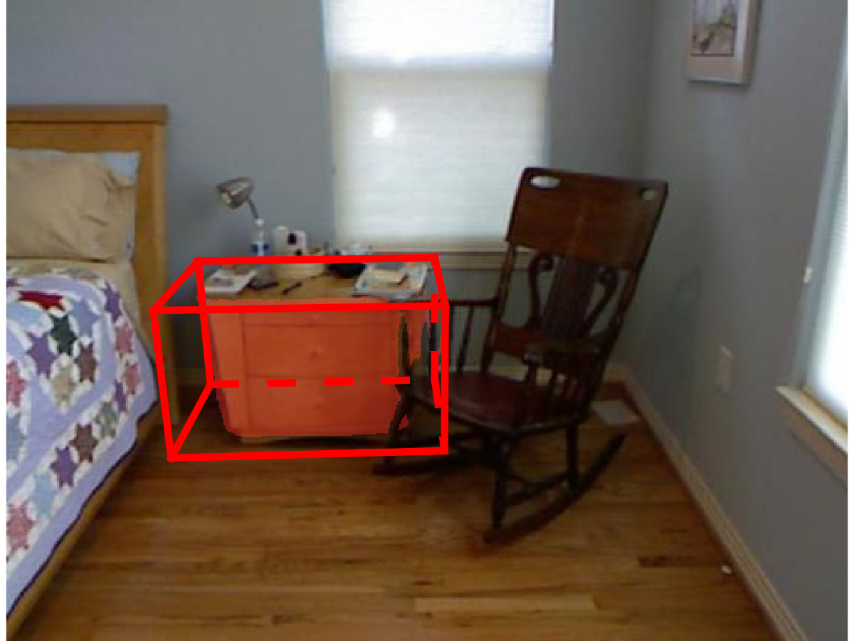
(1) chair (2) tv (3) bookshelf (4) sofa (5) bed (6) monitor (7) desk (8) night stand (9) garbage bin (10) box
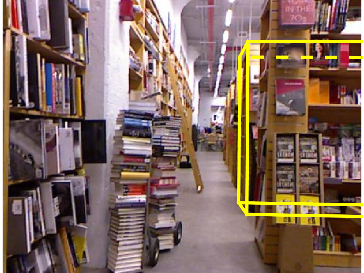
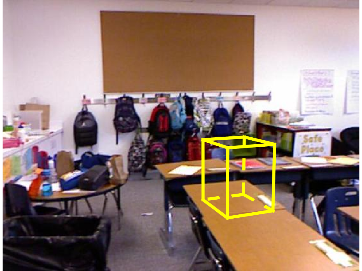
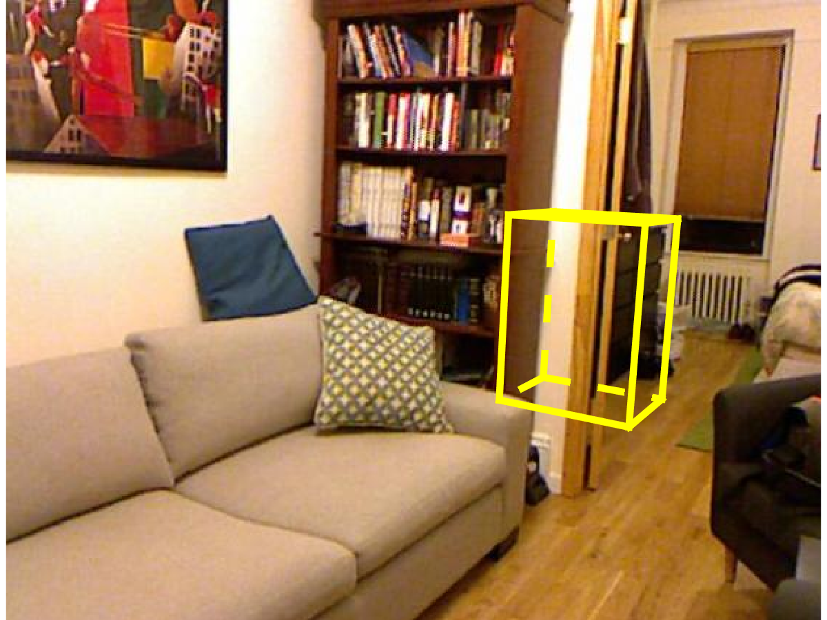
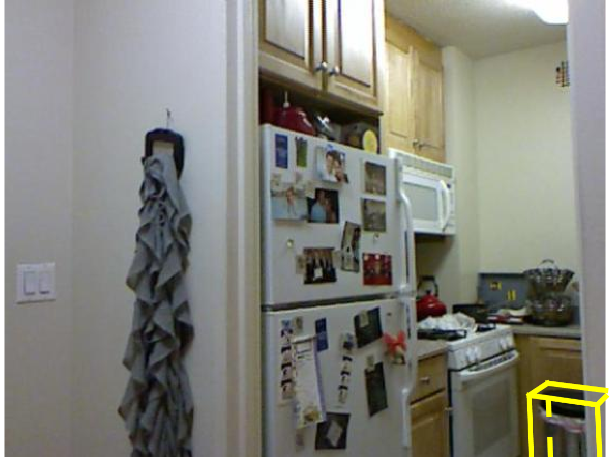
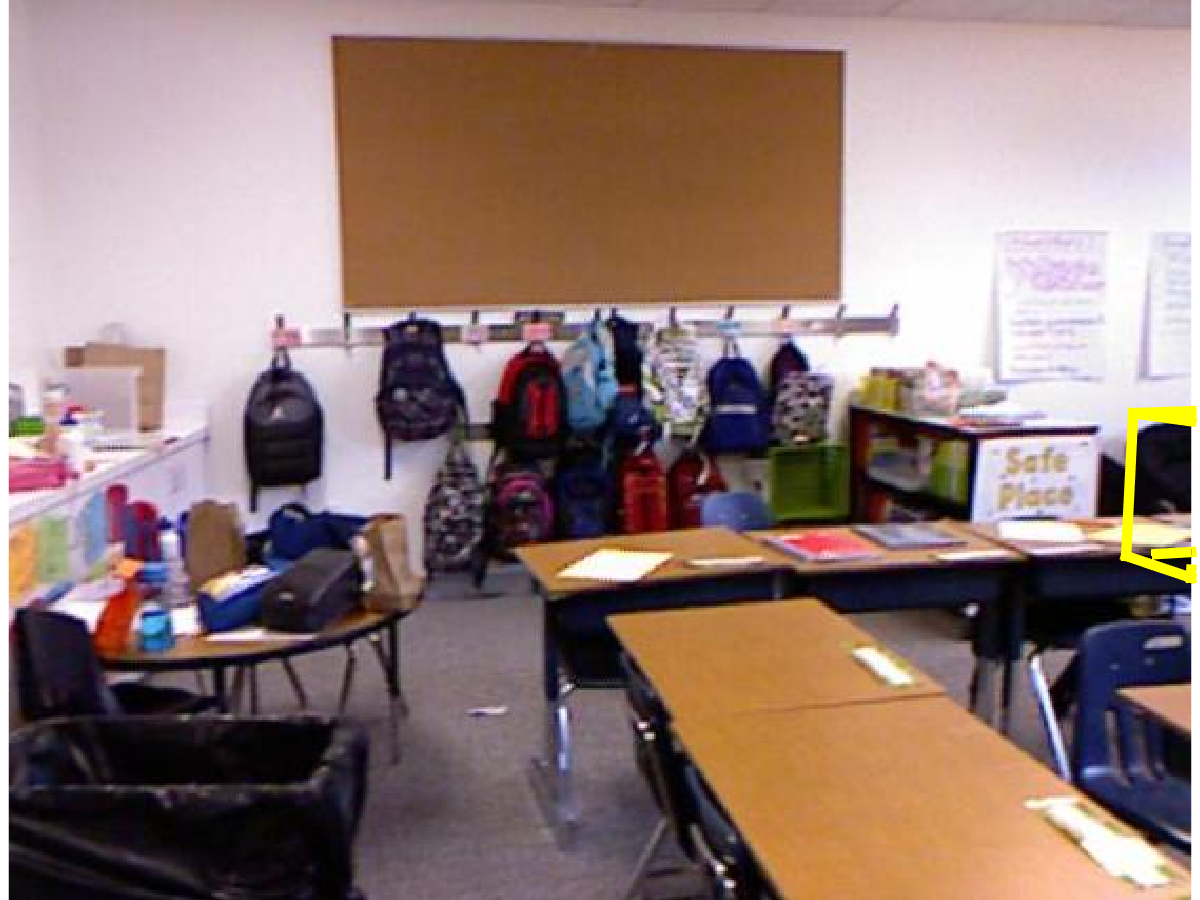
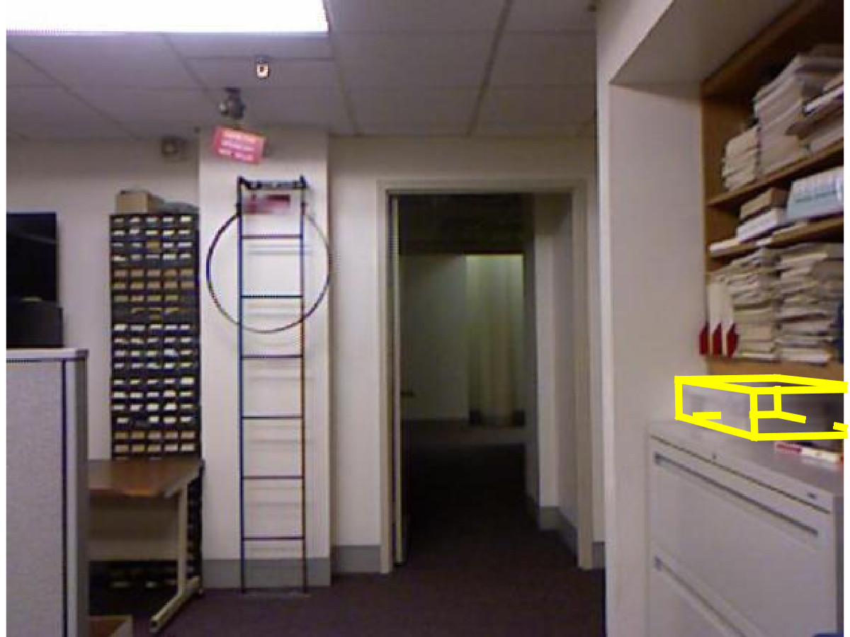
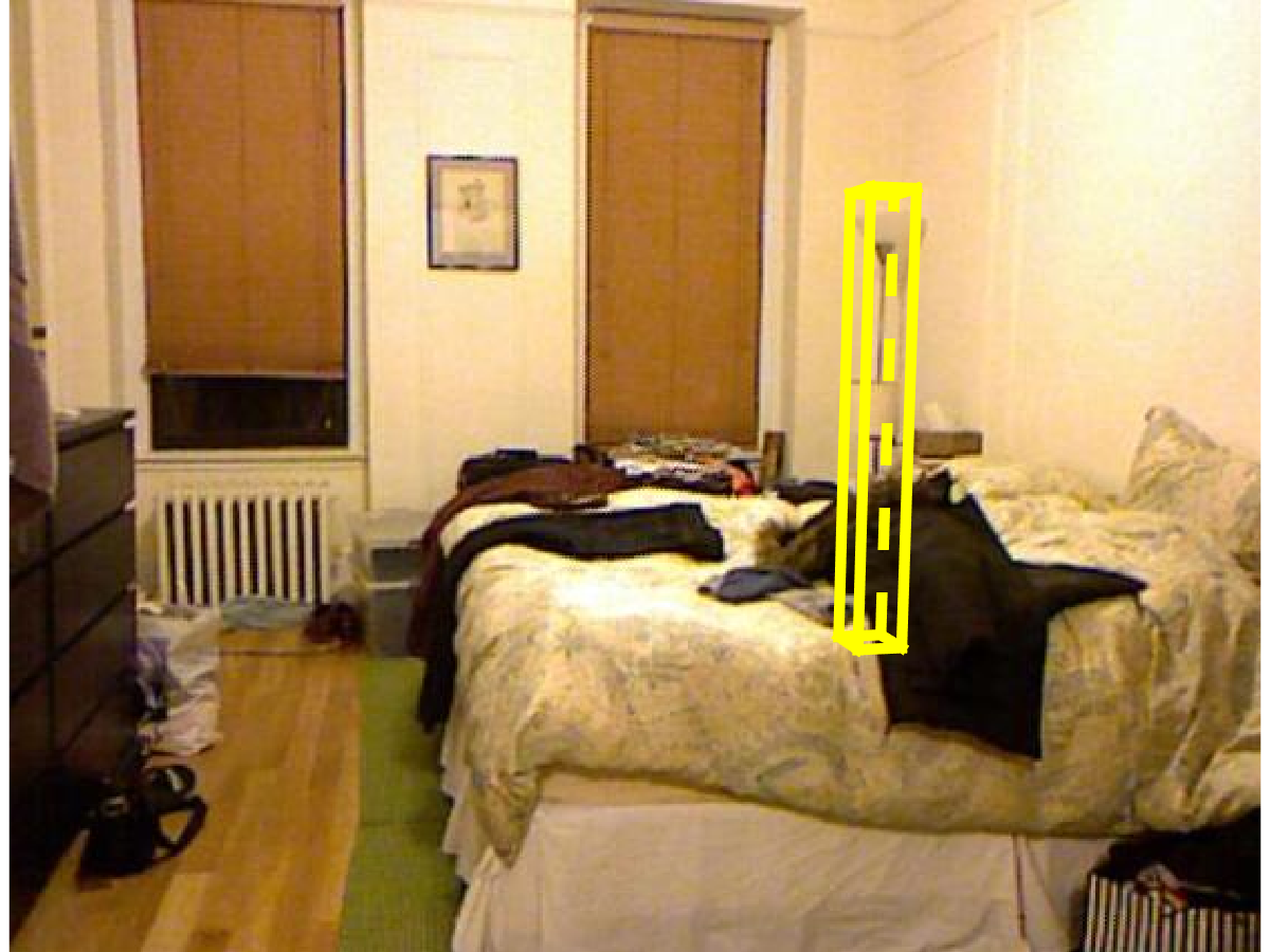
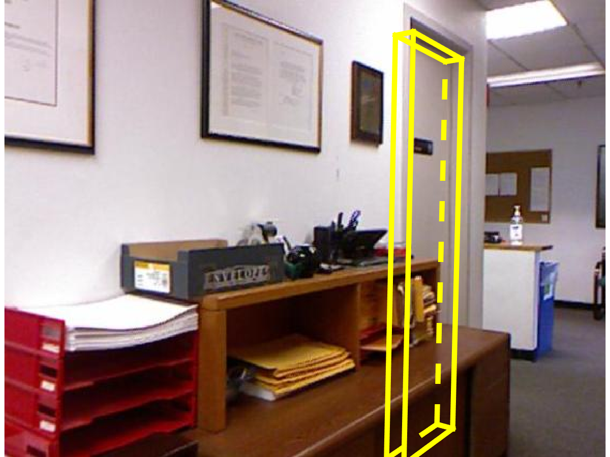
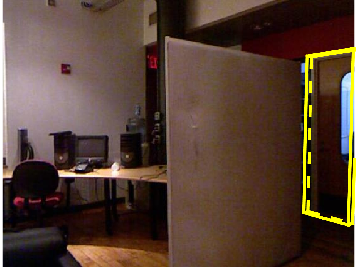
bookshelf chair dresser garbage bin sofa box lamp door door tv
4 Joint Amodal Object Recognition Network
Given the 3D proposal boxes, we feed the 3D space within each box to the Object Recognition Network (ORN). In this way, the final proposal feed to ORN could be the actual bounding box for the object, which allows the ORN to look at the full object to increase recognition performance, while still being computationally efficient. Furthermore, because our proposals are amodal boxes containing the whole objects at their full extent, the ORN can align objects in 3D meaningfully to be more invariant to occlusion or missing data for recognition. Figure 6 shows statistics of object sizes between amodal full box vs. modal tight box.
3D object recognition network
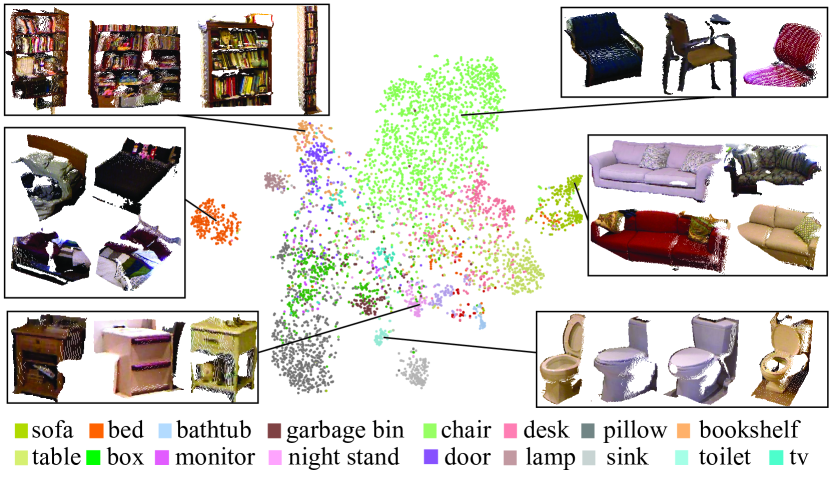
For each proposal box, we pad the proposal bounding box by of the sizes in each direction to encode some contextual information. Then, we divide the space into a voxel grid and use TSDF (Section 2) to encode the geometric shape of the object. The network architecture is shown in Figure 2. All the max pooling layers are with stride . For the three convolution layers, the window sizes are , , and , all with stride . Between the fully connected layers are ReLU and dropout layers (dropout ratio 0.5). Figure 10 visualizes the 2D t-SNE embedding of 5,000 foreground volumes using their the last layer features learned from the 3D ConvNet. Color encodes object category.
2D object recognition network
The 3D network only makes use of the depth map, but not the color. For certain object categories, color is a very discriminative feature, and existing ConvNets provide very powerful features for image-based recognition that could be useful to us. For each of the 3D proposal box, we project the 3D points inside the proposal box to 2D image plane, and find the tightest 2D box that contains all these 2D point projections. We use the state-of-the-art VGGnet [21] pre-trained on ImageNet [18] (without fine-tuning) to extract color features from the image. We use a Region-of-Interest Pooling Layer from Fast RCNN [6] to uniformly sample points from conv5_3 layer using the 2D window with one more fully connected layer to generate 4096-dimensional features as the feature from 2D images.
We also tried the alternative to encode color on 3D voxels, but it performs much worse than the pre-trained VGGnet (Table 2 [dxdydz+rgb] vs. [dxdydz+img]). This might be because encoding color in 3D voxel grid significantly lowers the resolution compared to the original image, and hence high frequency signal in the image get lost. In addition, by using the pre-trained model of VGG, we are able to leverage the large amount of training data from ImageNet, and the well engineered network architecture.
2D and 3D joint recognition
We construct a joint 2D and 3D network to make use of both color and depth. The feature from both 2D VGG Net and our 3D ORN (each has 4096 dimensions) are concatenated into one feature vector, and fed into a fully connected layer , which reduces the dimension to 1000. Another two fully connected layer take this feature as input and predict the object label and 3D box.
![[Uncaptioned image]](/html/1511.02300/assets/x8.png)
![[Uncaptioned image]](/html/1511.02300/assets/x9.png)
Multi-task loss
Similarly to RPN, the loss function consists of a classification loss and a 3D box regression loss:
| (2) |
where the is the predicted probability over 20 object categories (negative non-objects is labeled as class 0). For each mini-batch, we sample 384 examples from different images, with a positive to negative ratio of 1:3. For the box regression, each target offset is normalized element-wise with the object category specific mean and standard deviation.
SVM and 3D NMS
After training the network, we extract the features from FC3 and train a linear Support Vector Machine (SVM) for each object category. During testing, we apply 3D NMS on the results with threshold 0.1, based on their SVM scores. For box regressions, we directly use the results from the neural network.
Object size pruning
As shown in Figure 6, when we use amodal bounding boxes to represent objects, the bounding box sizes provide useful information about the object categories. To make use of this information, for each of the detected box, we check the box size in each direction, aspect ratio of each pair of box edge. We then compare these numbers with the distribution collected from training examples of the same category. If any of these values falls outside 1st to 99th percentile of the distribution, which indicates this box has a very different size, we decrease its score by 2.
5 Experiments
The training of RPN and ORN takes around 10 and 17 hours respectively on a NVIDIA K40 GPU. During testing, RPN takes 5.62s and ORN takes 13.93s per image, which is much faster than Depth RCNN (40s CPU + 30s GPU + expensive post alignment) and Sliding Shapes (25 mins number of object categories).
For the VGG network [21], we use the weights from [11] without fine tuning. To reduce GPU memory bandwidth, instead of storing as “float”, we use “half” to store both the network parameters and activations. We implement our own software framework from scratch using CUDA7.5 and CuDNN3 with FP16 support. The GPU memory usage is 5.41GB for RPN and 4.27GB for ORN (without VGGnet).
We evaluate our 3D region proposal and object detection algorithm on the standard NYUv2 dataset [20] and SUN RGB-D [SUNRGBD] dataset. The amodal 3D bounding box are obtained from SUN RGB-D dataset. We modified the rotation matrix from SUN RGB-D dataset to eliminate the rotation on x,y plane and only contains camera tilt angle. Following the evaluation metric in [23], we assume the all predictions and ground truth boxes are aligned in the gravity direction. We use 3D volume intersection over union between ground truth and prediction boxes, and use 0.25 as the threshold to calculate the average recall for proposal generation and average precision for detection.
5.1 Object Proposal Evaluation
Evaluation of object proposal on NYU dataset is shown in Table 1. On the left, we show the average recall over different IOUs. On the right, we show the recall for each object category with IOU threshold 0.25, as well as the average best overlap ratio (ABO) across all ground truth boxes. Table shows the evaluation on SUNRGB-D dataset.
Naïve 2D To 3D
Our first baseline is to directly lift 2D object proposal to 3D. We take the 2D object proposals from [9]. For each of them, we get the 3D points inside the bounding box (without any background removal), remove those outside 2 percentiles along all three directions, and obtain a tight fitting box around these inlier points. Obviously this method cannot predict amodal bounding box when the object is occluded or truncated, since 3D points only exist for the visible part of an object.
| poposal | algorithm | mAP | |||||||||||||||||||
| 3D SS | dxdydz no bbreg | 43.3 | 55.0 | 16.2 | 23.1 | 3.4 | 10.4 | 17.1 | 30.7 | 10.9 | 35.4 | 20.3 | 41.2 | 47.2 | 25.2 | 43.9 | 1.9 | 1.6 | 0.1 | 9.9 | 23.0 |
| dxdydz | 52.1 | 60.5 | 19.0 | 30.9 | 2.2 | 15.4 | 23.1 | 36.4 | 19.7 | 36.2 | 18.9 | 52.5 | 53.7 | 32.7 | 56.9 | 1.9 | 0.5 | 0.3 | 8.1 | 27.4 | |
| RPN | dxdydz no bbreg | 51.4 | 74.8 | 7.1 | 51.5 | 15.5 | 22.8 | 24.9 | 11.4 | 12.5 | 39.6 | 15.4 | 43.4 | 58.0 | 40.7 | 61.6 | 0.2 | 0.0 | 1.5 | 2.8 | 28.2 |
| dxdydz no svm | 58.9 | 79.8 | 15.7 | 56.3 | 11.3 | 20.3 | 18.8 | 16.5 | 18.2 | 38.1 | 15.1 | 54.0 | 57.7 | 47.2 | 66.8 | 1.3 | 0.0 | 0.6 | 8.3 | 30.8 | |
| dxdydz no size | 59.9 | 78.9 | 12.0 | 51.5 | 15.6 | 24.6 | 27.7 | 12.5 | 18.6 | 42.3 | 15.1 | 59.4 | 59.6 | 44.7 | 62.5 | 0.3 | 0.0 | 1.1 | 12.9 | 31.5 | |
| dxdydz | 59.0 | 80.7 | 12.0 | 59.3 | 15.7 | 25.5 | 28.6 | 12.6 | 18.6 | 42.5 | 15.3 | 59.5 | 59.9 | 45.3 | 64.8 | 0.3 | 0.0 | 1.4 | 13.0 | 32.3 | |
| tsdf dis | 61.2 | 78.6 | 10.3 | 61.1 | 2.7 | 23.8 | 21.1 | 25.9 | 12.1 | 34.8 | 13.9 | 49.5 | 61.2 | 45.6 | 70.8 | 0.3 | 0.0 | 0.1 | 1.7 | 30.2 | |
| dxdydz+rgb | 58.3 | 79.3 | 9.9 | 57.2 | 8.3 | 27.0 | 22.7 | 4.8 | 18.8 | 46.5 | 14.4 | 51.6 | 56.7 | 45.3 | 65.1 | 0.2 | 0.0 | 4.2 | 0.9 | 30.1 | |
| proj dxdydz+img | 58.4 | 81.4 | 20.6 | 53.4 | 1.3 | 32.2 | 36.5 | 18.3 | 17.5 | 40.8 | 19.2 | 51.0 | 58.7 | 47.9 | 71.4 | 0.5 | 0.2 | 0.3 | 1.8 | 32.2 | |
| dxdydz+img+hha | 55.9 | 83.0 | 18.8 | 63.0 | 17.0 | 33.4 | 43.0 | 33.8 | 16.5 | 54.7 | 22.6 | 53.5 | 58.0 | 49.7 | 75.0 | 2.6 | 0.0 | 1.6 | 6.2 | 36.2 | |
| dxdydz+img | 62.8 | 82.5 | 20.1 | 60.1 | 11.9 | 29.2 | 38.6 | 31.4 | 23.7 | 49.6 | 21.9 | 58.5 | 60.3 | 49.7 | 76.1 | 4.2 | 0.0 | 0.5 | 9.7 | 36.4 |
3D Selective Search
For 2D, Selective Search [25] is one of the most popular state-of-the-arts.
It starts with a 2D segmentation and uses hierarchical grouping to obtain the object proposals at different scales.
We study how well a similar method based on bottom-up grouping can work in 3D (3D SS).
We first use plane fitting on the 3D point cloud to get an initial segmentation.
For each big plane that covers more than of the total image area,
we use the RGB-D UCM segmentation from [10] (with threshold 0.2) to further split it.
Starting with on this over-segmentation, we hierarchically group [25] different segmentation regions,
with the following similarity measures:
measures color similarity between region and using histogram intersection on RGB color histograms;
, where is number of pixels in this region;
, where is the volume of 3D bounding boxes of the points in this region;
measures how well region and fit into each other to fill in gaps.
The final similarity measure is a weighted sum of these four terms.
To diversify our strategies, we run the grouping 5 times with different weights: .
For each of the grouped region, we will obtain two proposal boxes: one tight box and one box with height extended to the floor.
We also use the room orientation as the box orientation.
The room orientation and floor are obtained under the Manhattan world assumption described in Section 3.
After that we will remove the redundant proposals with 3D IOU greater than 0.9 by arbitrary selection.
Using both 3D and color, this very strong baseline achieves an average recall 74.2%.
But it is slow because of its many steps,
and the handcrafted segmentation and similarity might be difficult to tune optimally.
Our 3D RPN
Row 3 to 5 in Table 1 shows the performance of our 3D region proposal network. Row 3 shows the performance of single-scale RPN. Note that the recalls for small objects like lamp, pillow, garbage bin are very low. When one more scale is added, the performance for those small objects boosts significantly. Adding RGB color to the 3D TSDF encoding slightly improves the performance, and we use this as our final region proposal result. From the comparisons we can see that mostly planar objects (e.g. door) are easier to locate using segmentation-based selective search. Some categories (e.g. lamp) have a lower recall mostly because of lack of training examples. Table 2 shows the detection AP when using the same ORN architecture but different proposals (Row [3D SS: dxdydz] and Row [RPN: dxdydz]). We can see that the proposals provided by RPN helps to improve the detection performance by a large margin (mAP from 27.4 to 32.3).
5.2 Object Detection Evaluation
Feature encoding
From Row [RPN: dxdydz] to Row [RPN: dxdydz+img] in Table 2, we compare different feature encodings and reach the following conclusions. (1) TSDF with directions encoded is better than single TSDF distance ([dxdydz] vs. [tsdf dis]). (2) Accurate TSDF is better than projective TSDF ([dxdydz+img] vs. [proj dxdydz+img]). (3) Directly encoding color on 3D voxels is not as good as using 2D image VGGnet ([dxdydz+rgb] vs. [dxdydz+img]), probably because the latter one can preserve high frequency signal from images. (4) Adding HHA does not help, which indicates the depth information from HHA is already exploited by our 3D representation ([dxdydz+img+hha] vs. [dxdydz+img]).
| Algorithm | input | mAP | |||||
|---|---|---|---|---|---|---|---|
| Sliding Shapes [23] | d | 33.5 | 29 | 34.5 | 33.8 | 67.3 | 39.6 |
| [9] on instance seg | d | 71 | 18.2 | 49.6 | 30.4 | 63.4 | 46.5 |
| [9] on instance seg | rgbd | 74.7 | 18.6 | 50.3 | 28.6 | 69.7 | 48.4 |
| [9] on estimated model | d | 72.7 | 47.5 | 54.6 | 40.6 | 72.7 | 57.6 |
| [9] on estimated model | rgbd | 73.4 | 44.2 | 57.2 | 33.4 | 84.5 | 58.5 |
| ours [depth only] | d | 83.0 | 58.8 | 68.6 | 49.5 | 79.2 | 67.8 |
| ours [depth + img] | rgbd | 84.7 | 61.1 | 70.5 | 55.4 | 89.9 | 72.3 |
|
Recall |
ABO |
#Box |
||||||||||||||||||||
| 3D SS | 78.8 | 87.2 | 72.8 | 72.2 | 65.5 | 86.1 | 75.1 | 65.0 | 70.0 | 87.1 | 67.5 | 53.1 | 68.1 | 82.8 | 86.8 | 84.4 | 85.0 | 69.2 | 94.0 | 72.0 | 0.394 | 2000 |
| RPN | 98.1 | 99.1 | 79.5 | 51.5 | 93.3 | 89.2 | 94.9 | 24.0 | 87.0 | 79.6 | 62.0 | 41.2 | 96.2 | 77.9 | 96.7 | 97.3 | 96.7 | 63.3 | 100.0 | 88.7 | 0.485 | 2000 |
| mAP | ||||||||||||||||||||
| Sliding Shapes [23] | - | 42.09 | - | 33.42 | - | - | - | - | - | - | - | - | - | - | 23.28 | 25.78 | - | 61.86 | - | |
| Deep Sliding Shapes | 44.2 | 78.8 | 11.9 | 1.5 | 61.2 | 4.1 | 20.5 | 0.0 | 6.4 | 20.4 | 18.4 | 0.2 | 15.4 | 13.3 | 32.3 | 53.5 | 50.3 | 0.5 | 78.9 | 26.9 |
Design justification
We conducted several control experiments to understand the importance of each component.
Does bounding box regression help? Previous works have shown that box regression can significantly improve 2D object detection [6]. For our task, although we have depth, there is more freedom on 3D localization, which makes regression harder. We turn the 3D box regression on ([3DSS dxdydz], [RPN dxdydz]) and off ([3DSS dxdydz no bbreg], [RPN dxdydz no bbreg]). Whether we use 3D Selective Search or RPN for proposal generation, the 3D box regression always helps significantly (mAPs improve +4.4 and +4.1 respectively).
Does SVM outperform softmax? Instead of training one-vs-rest linear SVMs, we can also directly use the softmax score as detection confidence. Experiments in [6] shows that softmax slightly outperforms SVM. But in our case, using SVM improves the mAP by 0.5. This may be because SVM can better handle the unbalanced numbers of training examples among different categories in NYU.
Does size pruning help? Compared with and without the post-processing ([dxdydz] vs. [dxdydz no size]), we observe that for most categories, size pruning reduces false positives and improves the AP by the amount from 0.1 to 7.8, showing a consistent positive effect.
Is external training data necessary? Comparing to Sliding Shapes that uses extra CAD models, and Depth-RCNN that uses Image-Net for pre-training and CAD models for 3D fitting, our [depth only] 3D ConvNet does not require any external training data outside NYUv2 training set, and still outperforms the previous methods, which shows the power of 3D deep representation.
Comparison to the state-of-the-arts
We evaluate our algorithm on the same test set as [9] (The intersection of the NYUv2 test set and Sliding Shapes test set for the five categories being studied under “3D all” setting). Table 3 shows the comparison with the two state-of-the-arts for amodal 3D detection: 3D Sliding Shapes [23] with hand-crafted features, and 2D Depth-RCNN [9] with ConvNets features. Our algorithm outperforms by large margins with or without colors. Different from Depth-RCNN that requires fitting a 3D CAD model as post-processing, our method outputs the 3D amodal bounding box directly, and it is much faster. Table 5 shows the amodal 3D object detection results on SUN RGB-D dataset compared with Sliding Shapes [23].
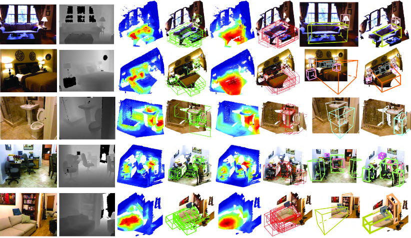
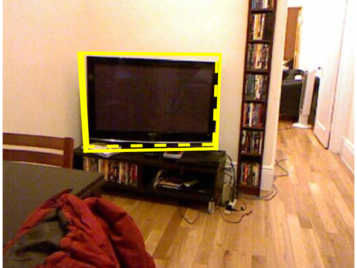
Figure 11 shows side-by-side comparisons to Sliding Shapes. First, the object proposal network and box regression provide more flexibility to detect objects with atypical sizes. For example, the small child’s chairs and table in the last row are missed by Sliding Shapes but detected by Deep Sliding Shape. Second, color helps to distinguish objects with similar shapes (e.g. bed vs. table). Third, the proposed algorithm can extend to many more object categories easily.
6 Conclusion
We present a 3D ConvNet pipeline for amodal 3D object detection, including a Region Proposal Network and a joint 2D+3D Object Recognition Network. Experiments show our algorithm significantly outperforms the state-of-the-art approaches, and is much faster than the original Sliding Shapes, which demonstrates the power of 3D deep learning for 3D shape representation.
Acknowledgment.
This work is supported by NSF/Intel VEC program. Shuran is supported by a Facebook fellowship. We thank NVIDIA and Intel for hardware donation. We thank Jitendra Malik and Thomas Funkhouser for valuable discussion.
References
- [1] P. Arbelaez, J. Pont-Tuset, J. Barron, F. Marques, and J. Malik. Multiscale combinatorial grouping. In CVPR, 2014.
- [2] L. Bo, X. Ren, and D. Fox. Unsupervised feature learning for RGB-D based object recognition. In ISER, 2013.
- [3] L. Bo, X. Ren, and D. Fox. Learning hierarchical sparse features for rgb-(d) object recognition. IJRR, 2014.
- [4] X. Chen, K. Kunku, Y. Zhu, A. Berneshawi, H. Ma, S. Fidler, and R. Urtasun. 3d object proposals for accurate object class detection. In NIPS, 2015.
- [5] Y. Fang, J. Xie, G. Dai, M. Wang, F. Zhu, T. Xu, and E. Wong. 3D deep shape descriptor. In CVPR, 2015.
- [6] R. Girshick. Fast R-CNN. ICCV, 2015.
- [7] R. Girshick, J. Donahue, T. Darrell, and J. Malik. Rich feature hierarchies for accurate object detection and semantic segmentation. In CVPR, 2014.
- [8] S. Gupta, P. Arbelaez, and J. Malik. Perceptual organization and recognition of indoor scenes from RGB-D images. In CVPR, 2013.
- [9] S. Gupta, P. A. Arbeláez, R. B. Girshick, and J. Malik. Aligning 3D models to RGB-D images of cluttered scenes. In CVPR, 2015.
- [10] S. Gupta, R. Girshick, P. Arbelaez, and J. Malik. Learning rich features from RGB-D images for object detection and segmentation. In ECCV, 2014.
- [11] S. Gupta, J. Hoffman, and J. Malik. Cross modal distillation for supervision transfer. arXiv, 2015.
- [12] H. Huang, E. Kalogerakis, and B. Marlin. Analysis and synthesis of 3D shape families via deep-learned generative models of surfaces. Computer Graphics Forum, 2015.
- [13] A. Kar, S. Tulsiani, J. Carreira, and J. Malik. Amodal completion and size constancy in natural scenes. In ICCV, 2015.
- [14] K. Lai, L. Bo, and D. Fox. Unsupervised feature learning for 3d scene labeling. In ICRA, 2014.
- [15] K. Lenc and A. Vedaldi. R-CNN minus R. BMVC, 2015.
- [16] D. Maturana and S. Scherer. VoxNet: A 3D convolutional neural network for real-time object recognition. In IROS, 2015.
- [17] S. Ren, K. He, R. Girshick, and J. Sun. Faster R-CNN: Towards real-time object detection with region proposal networks. NIPS, 2015.
- [18] O. Russakovsky, J. Deng, H. Su, J. Krause, S. Satheesh, S. Ma, Z. Huang, A. Karpathy, A. Khosla, M. Bernstein, et al. ImageNet large scale visual recognition challenge. IJCV, 2014.
- [19] B. Shi, S. Bai, Z. Zhou, and X. Bai. DeepPano: Deep panoramic representation for 3-D shape recognition. Signal Processing Letters, 2015.
- [20] N. Silberman, D. Hoiem, P. Kohli, and R. Fergus. Indoor segmentation and support inference from RGBD images. In ECCV, 2012.
- [21] K. Simonyan and A. Zisserman. Very deep convolutional networks for large-scale image recognition. arXiv, 2014.
- [22] R. Socher, B. Huval, B. Bhat, C. D. Manning, and A. Y. Ng. Convolutional-recursive deep learning for 3D object classification. In NIPS. 2012.
- [23] S. Song and J. Xiao. Sliding Shapes for 3D object detection in depth images. In ECCV, 2014.
- [24] H. Su, S. Maji, E. Kalogerakis, and E. G. Learned-Miller. Multi-view convolutional neural networks for 3D shape recognition. In ICCV, 2015.
- [25] J. R. Uijlings, K. E. van de Sande, T. Gevers, and A. W. Smeulders. Selective search for object recognition. IJCV, 2013.
- [26] T. Whelan, H. Johannsson, M. Kaess, J. J. Leonard, and J. McDonald. Robust real-time visual odometry for dense rgb-d mapping. In ICRA, 2013.
- [27] Z. Wu, S. Song, A. Khosla, F. Yu, L. Zhang, X. Tang, and J. Xiao. 3D ShapeNets: A deep representation for volumetric shapes. In CVPR, 2015.
- [28] J. Xie, Y. Fang, F. Zhu, and E. Wong. DeepShape: Deep learned shape descriptor for 3D shape matching and retrieval. In CVPR, 2015.
- [29] R. Zhile and E. B. Sudderth. Three-dimensional object detection and layout prediction using clouds of oriented gradients. In CVPR, 2016.
