Decay constants $f_{B}$ and $f_{B_{s}}$ from HISQ simulations

Abstract:

We give a progress report on a project aimed at a high-precision calculation of the decay constants $f_{B}$ and $f_{B_{s}}$ from simulations with HISQ heavy and light valence and sea quarks. Calculations are carried out with several heavy valence-quark masses on ensembles with 2+1+1 flavors of HISQ sea quarks at five lattice spacings and several light sea-quark mass ratios $m_{ud}/m_{s}$, including approximately physical sea-quark masses. This range of parameters provides excellent control of the continuum limit and of heavy-quark discretization errors. We present a preliminary error budget with projected uncertainties of 2.2 MeV and 1.5 MeV for $f_{B}$ and $f_{B_{s}}$, respectively.

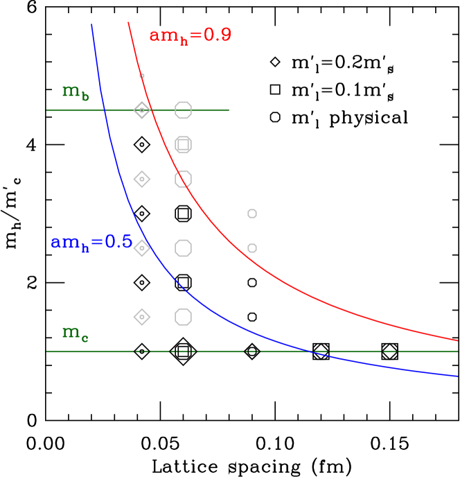
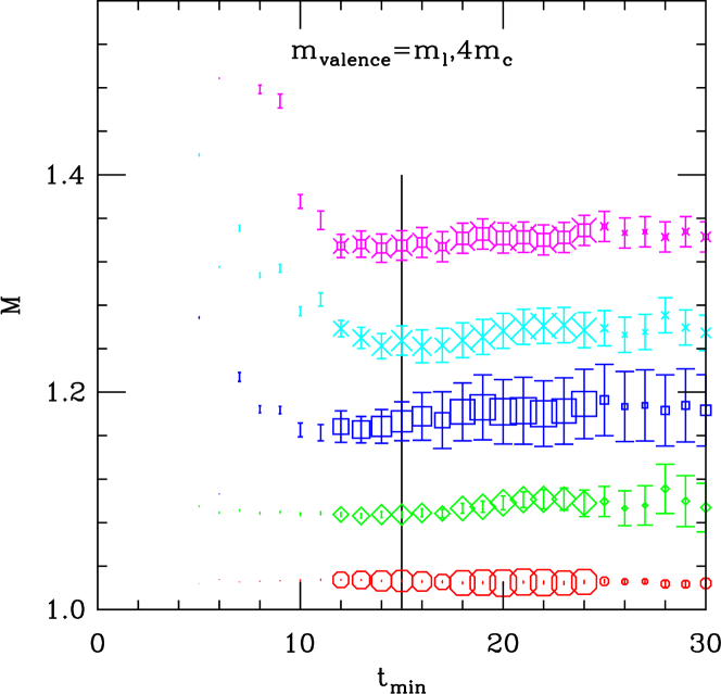
Figure 1: Left: heavy valence-quark masses and ensemble lattice spacings in this study for different light to strange sea-quark-mass ratios $m_{l}^{\prime}/m_{s}^{\prime}$. The symbol radius is proportional to the data sample size. The red line indicates the cut $am_{h}=0.9$; the blue, $am_{h}=0.5$. Faint symbols indicate omitted data. Right: Spectrum on the 0.042 fm physical-mass ensemble for a heavy-light meson with valence masses $4m_{c}^{\prime},m_{l}^{\prime}$ vs. $t_{\rm min}$, the minimum fit-range distance, with $m_{l}^{\prime}=m_{u}^{\prime}=m_{d}^{\prime}$. The symbol size is proportional to the $p$ value. The inset magnifies the ground state. Priors have been introduced to constrain the excited-state contributions. The vertical line shows our choice for $t_{\rm min}$.

1 Introduction

We are searching for new physics by looking for discrepancies between precise calculations within the Standard Model and high-precision experimental measurements. Here we provide a progress report on an effort to improve Standard-Model calculations of the leptonic decay constants of the $B$ and $B_{s}$ mesons, $f_{B}$ and $f_{B_{s}}$. These, in turn, provide accurate predictions for the charged-current leptonic decay $B\rightarrow\tau\nu$, for the FCNC decays $B_{s}\rightarrow\mu^{+}\mu^{-}$, and for neutral $B$ mixing. Such calculations are also needed to probe the $V-A$ structure of the $Wub$ vertex and to help address the present tension between inclusive and exclusive determinations of the CKM matrix element $|V_{ub}|$.

To achieve high precision, we employ highly improved staggered (HISQ) quarks [1, 2, 3] with masses heavier than the charm quark mass and adopt the HPQCD strategy of extrapolating to the $b$-quark mass [4]. The extrapolation is guided by heavy-quark effective theory, which we incorporate in our chiral/continuum analysis.

We reduce errors from previous calculations for three reasons. The staggered-fermion local pseudoscalar density does not require renormalization, one of the significant sources of systematic error with other heavy-quark formalisms [5, 6, 7, 8, 9]. Compared with HPQCD, our ensembles employ HISQ instead of asqtad sea quarks. The HISQ ensembles [10] have a large statistical sample size, and include lattices with nearly physical-mass light quarks, which reduces significantly chiral extrapolation errors.

This work extends our earlier calculation of $f_{D}$, $f_{D_{s}}$, which also used the HISQ formalism for charm quarks [11]. Here we include valence fermions heavier than charm.

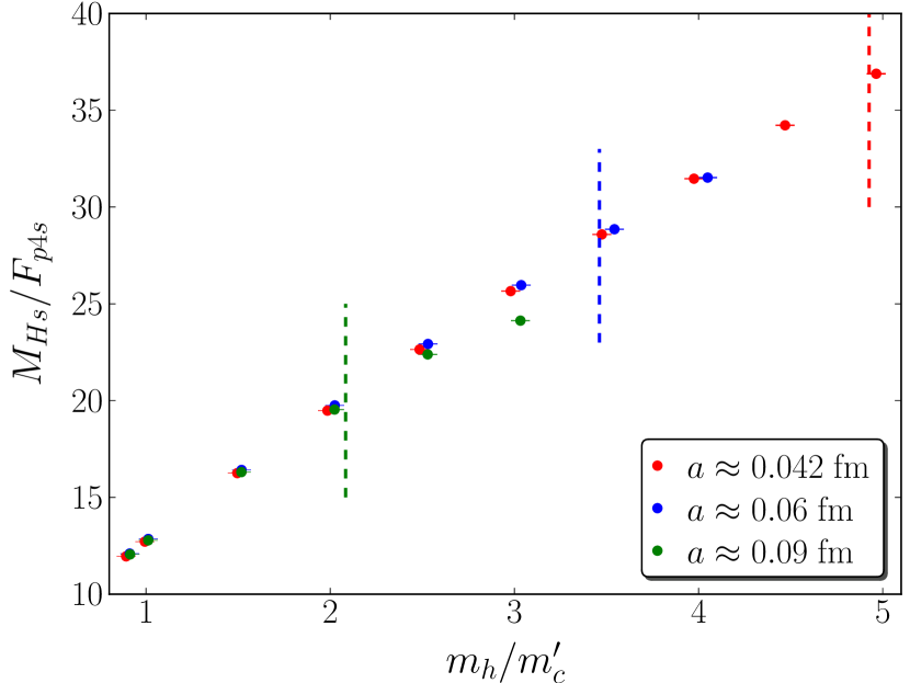
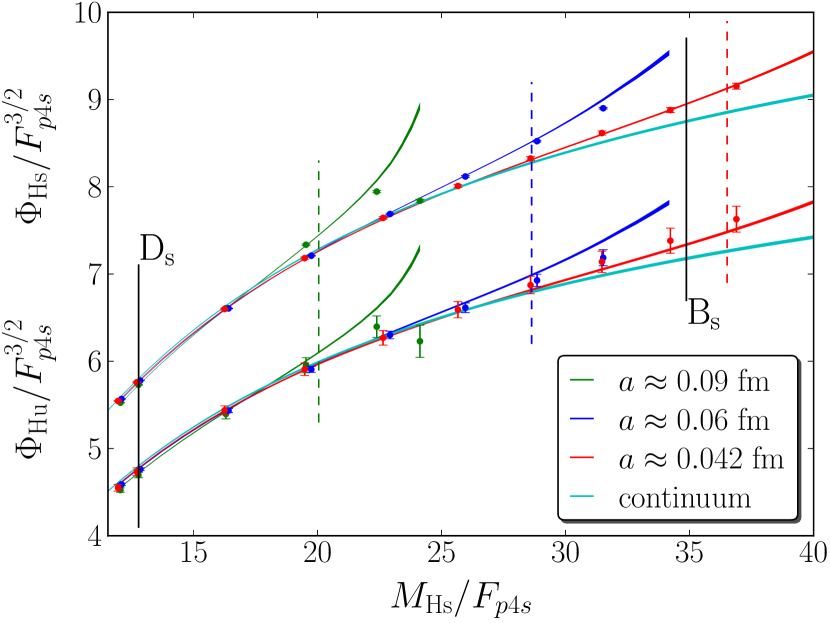
Figure 2: Illustration of heavy-quark discretization effects. Left: heavy-strange meson mass in units of $F_{p4s}\approx 154$ MeV vs. the ratio of the heavy-quark mass to the simulation charm quark mass $m_{h}/m_{c}^{\prime}$ for three lattice spacings at physical sea-quark masses. The small differences in the heavy-strange mass for different lattice spacings gives an indication of the heavy-quark discretization error. Right: decay constants $\Phi_{H_{q}}$ (defined below) plotted in units of $F_{p4s}$ vs. the heavy-strange meson mass for three lattice spacings and the continuum extrapolation. In both cases the dashed vertical lines indicate the cut $am_{h}=0.9$ for each lattice spacing. Such a pattern of deviations was first reported by HPQCD [4].

The range of valence heavy-quark masses and lattice spacings for the HISQ ensembles in this study is indicated in the left panel of Fig. 1. HISQ quarks show large lattice artifacts in the meson dispersion relations when $am_{h}>0.9$. Discretization effects in the heavy-light meson mass and decay constant, shown in Fig. 2, also increase dramatically for larger $am_{h}$. So we drop data with $am_{h}>0.9$ and parameterize the heavy-quark mass dependence in our fits at smaller values with the help of heavy-quark effective theory. Because of strong correlations, we also discard some $m_{h}/m_{c}^{\prime}$ points. (Primes on the masses indicate the simulation mass values.)

An important question is whether at the smallest lattice spacings our ensembles are ergodic with respect to the topological charge. In Fig. 3 we show the evolution of topological charge for our 0.06 fm and 0.042 fm ensembles. It is clear that tunneling has slowed at the smaller lattice spacing. Tunneling is less frequent when the light sea quark is unphysically heavy. We are currently investigating the implications for various observables.

2 Correlator Analysis

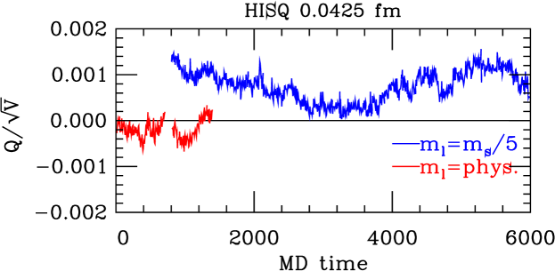
Figure 3: Topological charge vs. molecular dynamics time unit. Only fluctuations in $Q^{2}$ are relevant for the (parity-conserving) matrix elements here.

We compute the decay constant from the asymptotic behavior of the heavy-light pseudoscalar density-density correlator in the usual way:

$$C_{\rm pt-pt}(t)\rightarrow A_{\rm pt-pt}\exp(-M_{H_{q}}t)$$ (1)

where $M_{H_{q}}$ is the heavy-light meson mass and $q$ labels the light valence quark. The decay constant is then obtained without the need for matching factors from

$$f_{H_{q}}=(m_{h}+m_{q})\sqrt{\frac{3VA_{\rm pt-pt}}{2M^{3}_{H_{q}}}}$$ (2)

The correlators are calculated with random and Coulomb-gauge wall sources and point sinks. We compared fits to 3+2 states (3 nonoscillating and 2 oscillating) and to 2+1 states and conclude that 3+2 states incorporate adequately the effects of excited states. We can get a sense of the stability of the 3+2 fit from a plot of the resulting spectrum of ground and excited states as a function of $t_{\rm min}$, shown in the right panel of Fig. 1 for the 0.042 fm, physical-mass ensemble.

3 Chiral-continuum Extrapolation

We use heavy-quark effective theory (HQET) to model the heavy-quark mass dependence of $f_{H_{q}}$. We start by relating the QCD current to the HQET current:

$$J^{\rm QCD}\equiv C_{i}(m_{Q}/\mu,\alpha_{s}(\mu))J^{\rm HQET}_{i}(\mu)+{\cal O}(1/m_{Q})\,,$$ (3)

where the Wilson coefficient has the perturbative expression

$$C_{i}(m_{Q}/\mu,\alpha_{s}(\mu))=\left[\frac{\alpha_{S}(m_{Q})}{\alpha_{S}(\mu)}\right]^{-6/25}\left[1+{\cal O}\left(\alpha_{S}(m_{Q}),\alpha_{S}(\mu)\right)\right]\,.$$ (4)

So, with $M_{H_{s}}$ at physical sea-quark masses and physical valence $s$-quark mass, we remove the scaling factors from the decay constant and write it in terms of $\Phi_{H_{q}}$:

$$f_{H_{q}}\sqrt{M_{H_{q}}} = \Phi_{H_{q}}=\left[\alpha_{S}(M_{H_{s}})\right]^{-6/25}\left[1+{\cal O}\left(\alpha_{S}(M_{H_{s}})\right)\right]\ \tilde{\Phi}_{H_{q}}\,,$$

$$\tilde{\Phi}_{H_{q}} = \tilde{\Phi}_{0}\left(1+k_{1}\frac{\Lambda_{\rm\small HQET}}{M_{H_{s}}}+k_{2}\frac{\Lambda_{\rm\small HQET}^{2}}{M_{H_{s}}^{2}}+k_{1}^{\prime}\frac{\Lambda_{\rm\small{HQET}}}{m_{c}^{\prime}}\right)\left(1+\mbox{\rm log/analytic terms}\right)\,.\quad$$ (5)

We then introduce the heavy-quark discretization correction for the low energy constant $\Phi_{0}$ following HPQCD [4]

$$\tilde{\Phi}_{0}\rightarrow\tilde{\Phi}_{0}[1+c_{1}\alpha_{S}(a\Lambda)^{2}+c_{2}(a\Lambda)^{4}+c_{3}\alpha_{S}(am_{h})^{2}+c_{4}(am_{h})^{4}+\ldots{}]\,.$$ (6)

Finally, for the chiral logarithms and analytic terms in Eq. (5), we use heavy-meson rooted all-staggered $\chi$PT from Bernard and Komijani [12], which parameterizes the light-quark mass dependence and incorporates taste-breaking and generic discretization errors from the light-quark and gluon actions. Because of space limitations we give only a schematic representation:

$$(1+\mbox{\rm log/analytic terms}) = 1+\mbox{\rm NLO staggered chiral logarithms}$$ (7)

$$+$$ NLO + NNLO + NNNLO analytic terms

NLO analytic terms $$= \left(L_{s}+L_{s,M}\frac{\Lambda_{\rm\small HQET}}{M_{H_{s}}}\right)\left(2m_{l}+m_{s}\right)+\left(L_{q}+L_{q,M}\frac{\Lambda_{\rm\small HQET}}{M_{H_{s}}}\right)\left(m_{q}\right)+c_{a,\Xi}a^{2}\ .$$

Note that the coefficients of the NLO analytic terms include a heavy-quark mass correction. A heavy-quark mass dependence also appears implicitly through the $M_{H_{q}^{*}}-M_{H_{q}}$ hyperfine splitting and heavy-light flavor splittings.

Altogether our HQET-chiral continuum-chiral function, Eq. (5) with Eqs. (6) and (7) including NLO, NNLO, and NNNLO terms has 26 parameters. We use this parameterization for our central fit to our values of $\Phi_{H_{q}}$. An example of the resulting fit is shown in the left panel of Fig. 4. From the continuum extrapolation, we obtain values of the decay constants as a function of $M_{H_{s}}$ and the light valence-quark mass.

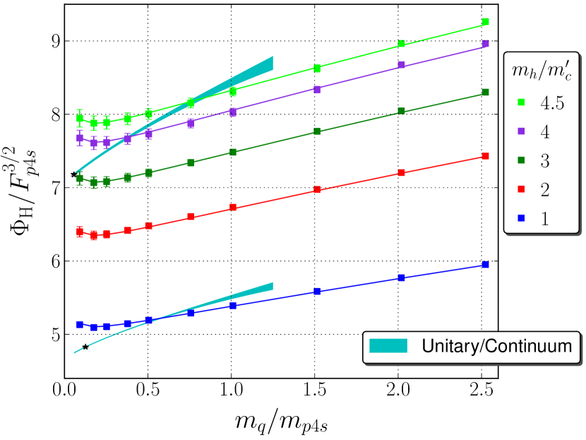
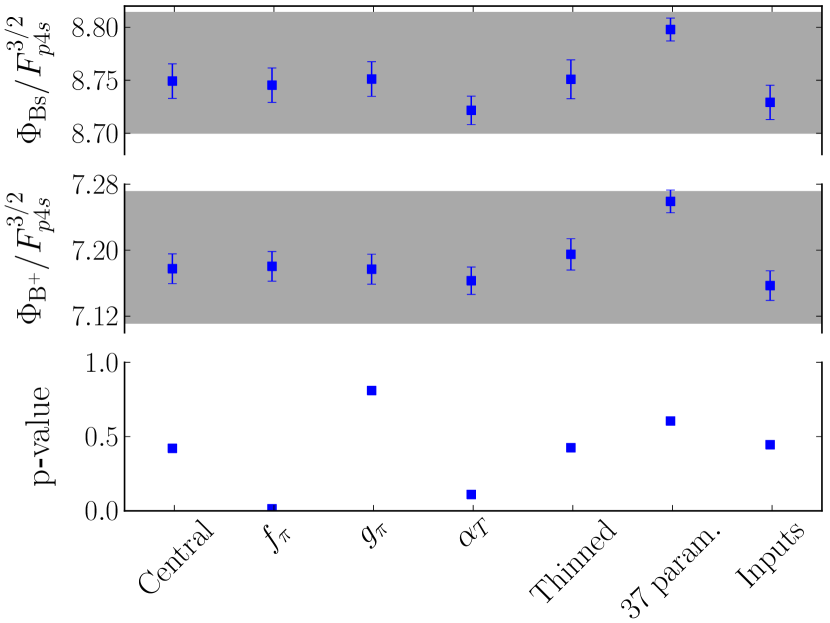
Figure 4: Left: sample chiral-continuum fit result for the $a\approx 0.042$ fm, $m^{\prime}_{l}/m^{\prime}_{s}=0.2$ data. The unitary/continuum result at physical $s$-, $c$-, and $b$-quark masses is shown in cyan. The stars indicate the fully physical results for the $B^{+}$ and $D^{+}$ mesons. Right: stability plot showing the sensitivity to model choices as described in the text. The error band shows the error taken for systematics associated with the chiral-continuum fit.

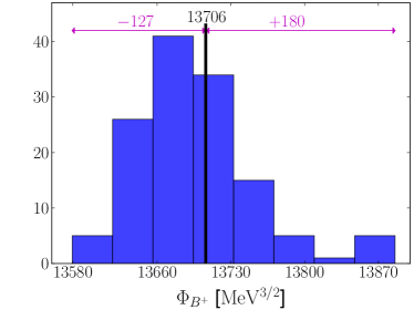
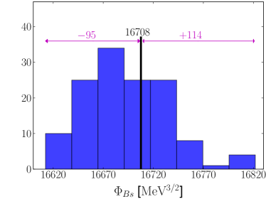
Figure 5: Histogram of central values resulting from varying choices of the fit function and input data. We estimate the associated systematic error from the extrema.

4 Error Budget

To estimate the systematic error in our methodology arising from the variety of possible analysis choices and to test the stability of our results, we tried the following alternatives. (1) Replaced $f_{K}$ with $f_{\pi}$ in the chiral terms; (2) Let the $B^{*}-B-\pi$ coupling $g_{\pi}$ that enters the chiral logarithms float with a prior 0.53(8). (3) Replaced $\alpha_{S}$ with a value determined empirically from the measured taste splittings. (4) Dropped half the light quark masses and refit; (5) Increased the number of parameters to 37 by adding 11 higher-order heavy-quark terms and do not make any SVD cuts in the fit. (6) Used an alternative determination of the $F_{p4s}$ scale and quark-mass ratios.

The effect of these variations on the decay constant is plotted in the right panel of Fig. 4. Selecting 132 combinations of such variations that yielded $p>0.05$ gives us the histograms shown in Fig. 5 for $\Phi_{B}$ and $\Phi_{B_{s}}$. We take the extrema of the histograms as the systematic error, noting that the majority of fit variations lie well within this conservative choice. The result is shown in the preliminary error budget in Table 1. The remaining sub-dominant systematic uncertainties from finite-volume effects, electromagnetic effects, and the experimental error in $f_{\pi}$ used to set the absolute lattice scale are estimated following Ref. [11]. Adding these errors in quadrature gives the estimated total uncertainty shown there.

Table 1: Preliminary error budget. Note that the first error, estimated from the histogram in Fig. 5, includes the chiral-continuum fit and $g_{\pi}$ errors, the light- and heavy-quark discretization errors, and the error arising from excited state contamination.

	$f_{B^{+}}$ (MeV)	$f_{B_{s}}$ (MeV)
$\chi$PT$\oplus g_{\pi}\oplus$ HQ-LQ disc. $\oplus$ 2-pt fit	2.1	1.4
Statistics	0.6	0.5
Finite volume	0.3	0.2
Electromagnetic effects	0.1	0.1
Exp. $f_{\pi}$	0.3	0.4
Total	2.2	1.5

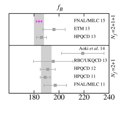
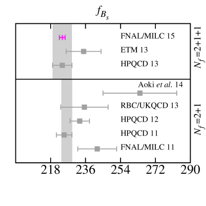
Figure 6: Comparison with other recent results [4, 5, 6, 7, 8, 9, 13]. Vertical bands show the recent PDG lattice averages [14]. Here we illustrate only our projected error, and take the (2+1+1)-flavor average as our central value.

5 Results and Outlook

We have presented the status of our analysis of $f_{B}$ and $f_{B_{s}}$ from a calculation with all HISQ quarks using the HPQCD scheme of extrapolating from lighter heavy-quark masses to the $b$-quark mass. In Fig. 6 we compare our projected total error with the recent compilation of results from the Particle Data Group [14]. We anticipate that our calculations when completed will be the most precise to date. We are presenty generating and analyzing a 0.03 fm, ($m^{\prime}_{l}/m^{\prime}_{s}=0.2$) ensemble for which $am_{b}=0.6$. Here no extrapolation from lighter heavy-quark masses is needed.

- [1] E. Follana et al. [HPQCD], Phys. Rev. D 75, 054502 (2007) [hep-lat/0610092].
- [2] A. Bazavov et al. \posPoS(LATTICE 2008)033 (2008) [arXiv:0903.0874]; \posPoS(LAT2009)123 (2009), [arXiv:0911.0869]; \posPoS(Lattice 2010)320 (2010), [arXiv:1012.1265].
- [3] A. Bazavov et al. [MILC], Phys. Rev. D 82, 074501 (2010) [arXiv:1004.0342].
- [4] C. McNeile et al. [HPQCD], Phys. Rev. D 85, 031503 (2012) [arXiv:1110.4510 [hep-lat]].
- [5] A. Bazavov et al., Phys. Rev. D 85, 114506 (2012) [arXiv:1112.3051 [hep-lat]].
- [6] H. Na et al. [HPQCD] Phys. Rev. D 86, 034506 (2012) [arXiv:1202.4914 [hep-lat]].
- [7] R. J. Dowdall et al. [HPQCD], Phys. Rev. Lett. 110, no. 22, 222003 (2013) [arXiv:1302.2644 [hep-lat]].
- [8] N. H. Christ et al. [RBC/UKQCD] Phys. Rev. D 91, no. 5, 054502 (2015) [arXiv:1404.4670 [hep-lat]].
- [9] Y. Aoki, T. Ishikawa, T. Izubuchi, C. Lehner and A. Soni, Phys. Rev. D 91, no. 11, 114505 (2015) [arXiv:1406.6192 [hep-lat]].
- [10] A. Bazavov et al. [MILC], Phys. Rev. D 87, 054505 (2013) [arXiv:1212.4768].
- [11] A. Bazavov et al., Phys. Rev. D 90, 074509 (2014) [arXiv:1407.3772 [hep-lat]].
- [12] C. Bernard and J. Komijani, Phys. Rev. D 88, 094017 (2013) [arXiv:1309.4533 [hep-lat]].
- [13] N. Carrasco et al., \posPoS(LATTICE 2013)313 (2014) [arXiv:1311.2837 [hep-lat]].
- [14] J. L. Rosner, S. Stone and R. S. Van de Water, arXiv:1509.02220 [hep-ph].