Signed Support Recovery for Single Index Models in High-Dimensions

Matey Neykov Department of Operations Research and Financial Engineering, Princeton University, Princeton, NJ 08544    Qian Lin Center of Mathematical Sciences and Applications, Harvard University, Cambridge, MA 02138    Jun S. Liu Department of Statistics, Harvard University, Cambridge, MA 02138
Abstract

In this paper we study the support recovery problem for single index models Y=f(𝑿𝜷,ε)𝑌𝑓superscript𝑿𝜷𝜀Y=f(\boldsymbol{X}^{\intercal}\boldsymbol{\beta},\varepsilon), where f𝑓f is an unknown link function, 𝑿Np(0,𝕀p)similar-to𝑿subscript𝑁𝑝0subscript𝕀𝑝\boldsymbol{X}\sim N_{p}(0,\mathbb{I}_{p}) and 𝜷𝜷\boldsymbol{\beta} is an s𝑠s-sparse unit vector such that 𝜷i{±1s,0}subscript𝜷𝑖plus-or-minus1𝑠0\boldsymbol{\beta}_{i}\in\{\pm\frac{1}{\sqrt{s}},0\}. In particular, we look into the performance of two computationally inexpensive algorithms: (a) the diagonal thresholding sliced inverse regression (DT-SIR) introduced by Lin et al. (2015); and (b) a semi-definite programming (SDP) approach inspired by Amini & Wainwright (2008). When s=O(p1δ)𝑠𝑂superscript𝑝1𝛿s=O(p^{1-\delta}) for some δ>0𝛿0\delta>0, we demonstrate that both procedures can succeed in recovering the support of 𝜷𝜷\boldsymbol{\beta} as long as the rescaled sample size Γ=nslog(ps)Γ𝑛𝑠𝑝𝑠\Gamma=\frac{n}{s\log(p-s)} is larger than a certain critical threshold. On the other hand, when ΓΓ\Gamma is smaller than a critical value, any algorithm fails to recover the support with probability at least 1212\frac{1}{2} asymptotically. In other words, we demonstrate that both DT-SIR and the SDP approach are optimal (up to a scalar) for recovering the support of 𝜷𝜷\boldsymbol{\beta} in terms of sample size. We provide extensive simulations, as well as a real dataset application to help verify our theoretical observations.

Keywords: Single index models, Sliced inverse regression, Sparsity, Support recovery, High-dimensional statistics, Semidefinite programming

1 Introduction

Due to the recent advances in technology, collecting data becomes a routine. The ‘small n𝑛n, large p𝑝p’ characteristic of modern data brings new challenges in interpreting and processing it. Dimension reduction and variable selection procedures become an indispensable step in data exploration. Regrettably, the majority of the classical algorithms were developed to work in the regime pnmuch-less-than𝑝𝑛p\ll n, and hence one needs to exercise caution when applying existing methods in a high dimensional setting. A firm understanding of the limitations of classical dimension reduction procedures in the modern pnmuch-greater-than𝑝𝑛p\gg n regime, will help facilitate their appropriate application.

For example, the archetypical unsupervised dimension reduction procedure — principal component analysis (PCA), has been widely and successfully applied in a range of scientific problems (Price et al., 2010; Brenner et al., 2000, e.g.). The behavior of PCA in high dimensions has been well studied in the recent years. In Johnstone & Lu (2004, 2009); Paul (2007), it was shown that in the spiked covariance model, PCA succeeds if and only if limpn0𝑝𝑛0\lim\frac{p}{n}\neq 0. This result stimulated the statistical community to discuss the minimax rate of estimating the principal space under sparsity constraints (see e.g., Cai et al. (2013); Vu & Lei (2012) and references therein) and the tradeoff between the statistical and computational efficiency (see e.g., Berthet & Rigollet (2013)).

Another line of dimension reduction research, studies the so-called sufficient dimension reduction (SDR). The goal of SDR is to find the minimal subspace 𝒮𝒮\mathcal{S} such that Y𝑿|P𝒮𝑿Y\perp\!\!\!\perp\boldsymbol{X}\big{|}P_{\mathcal{S}}\boldsymbol{X}, where 𝑿p𝑿superscript𝑝\boldsymbol{X}\in\mathbb{R}^{p} is the predictor vector and Y𝑌Y\in\mathbb{R} is the response (Cook et al., 2004; Li, 1991; Cook & Ni, 2005, e.g.). Unlike its unsupervised counterpart, much less attention has been paid to how SDR algorithms behave in a high dimensional setting. The optimal estimation rates of SDR algorithms in terms of sparsity (s𝑠s), dimensionality (p𝑝p), and sample size (n𝑛n) are unclear.

Sliced inverse regression, proposed by Li (1991), is one of the most popular SDR methods for estimating the space 𝒮𝒮\mathcal{S}. When the dimensionality p𝑝p is larger than or comparable to the sample size n𝑛n, sparsity assumptions are often imposed on the loading vector 𝜷𝜷\boldsymbol{\beta} (Li & Nachtsheim, 2006, e.g.). Lin et al. (2015) proved that in fact 𝔼[(𝜷^,𝜷)]>0𝔼delimited-[]^𝜷𝜷0\mathbb{E}[\angle(\widehat{\boldsymbol{\beta}},\boldsymbol{\beta})]>0 if ρ=limpn0𝜌𝑝𝑛0\rho=\lim\frac{p}{n}\neq 0 and sin((𝜷^,𝜷))=0^𝜷𝜷0\sin\big{(}\angle(\widehat{\boldsymbol{\beta}},\boldsymbol{\beta})\big{)}=0 when ρ=0𝜌0\rho=0 where 𝜷^^𝜷\widehat{\boldsymbol{\beta}} is the SIR estimator of 𝜷𝜷\boldsymbol{\beta}. In other words, the SIR estimator 𝜷^^𝜷\widehat{\boldsymbol{\beta}} is consistent (up to a sign) if and only if ρ=limpn=0𝜌𝑝𝑛0\rho=\lim\frac{p}{n}=0. One implication of this result is that in order to estimate 𝜷𝜷\boldsymbol{\beta}, structural assumptions such as sparsity are necessary in the high dimensional setting.

In the present paper, inspired by Amini & Wainwright (2008), we investigate the support recovery problem for single index models (SIM) (1), under the sparsity assumption 𝜷0=ssubscriptnorm𝜷0𝑠\|\boldsymbol{\beta}\|_{0}=s in the regime s=O(p1δ)𝑠𝑂superscript𝑝1𝛿s=O(p^{1-\delta}) for some δ>0𝛿0\delta>0. More formally we study the models:

Y=f(𝑿𝜷,ε) with 𝑿Np(0,𝕀p),𝑌𝑓superscript𝑿𝜷𝜀 with 𝑿similar-tosubscript𝑁𝑝0subscript𝕀𝑝Y=f(\boldsymbol{X}^{\intercal}\boldsymbol{\beta},\varepsilon)\mbox{ with }\boldsymbol{X}\sim N_{p}(0,\mathbb{I}_{p}), (1)

where the noise ε𝜀\varepsilon is independent of 𝑿𝑿\boldsymbol{X} and f,ε,𝜷𝑓𝜀𝜷f,\varepsilon,\boldsymbol{\beta} belong to the class:

A={(f,ε,𝜷)\displaystyle\mathcal{F}_{A}=\Big{\{}(f,\varepsilon,\boldsymbol{\beta}) :Var(𝔼[Z|f(Z,ε)])A where ZN(0,1),:absentVar𝔼delimited-[]conditional𝑍𝑓𝑍𝜀𝐴 where 𝑍similar-to𝑁01\displaystyle:\operatorname{Var}(\mathbb{E}[Z|f(Z,\varepsilon)])\geq A\mbox{ where }Z\sim N(0,1), (2)
𝜷i{±1s,0} and (f,ε) is sliced stable (see Definition 1)}.\displaystyle\boldsymbol{\beta}_{i}\in\Big{\{}\pm\frac{1}{\sqrt{s}},0\Big{\}}\mbox{ and }(f,\varepsilon)\mbox{ is {sliced stable} (see Definition \ref{def:sliced_stable})}\Big{\}}.

Notice that no generality is lost in assuming that the vector 𝜷𝜷\boldsymbol{\beta} is a unit vector since otherwise model (1) is not identifiable. Model class (2), further assumes the idealized setting where all non-zero coordinates of 𝜷𝜷\boldsymbol{\beta} have a signal strength of exactly the same magnitude, which simplifies our presentation while preserving the inherent complexity of the support recovery problem. We believe that studying support recovery in SIM, would bring us insightful understanding of SIR and other SDR algorithms.

In this paper, we study two procedures for signed support recover of SIM (1): the DT-SIR introduced by Lin et al. (2015) and the SDP approach inspired by Amini & Wainwright (2008). We let Γ=nslog(ps)Γ𝑛𝑠𝑝𝑠\Gamma=\frac{n}{s\log(p-s)} be the rescaled sample size. Our main contribution is to establish the existence of constants ω>0𝜔0\omega>0 and Ω>0Ω0\Omega>0 such that when Γ>ΩΓΩ\Gamma>\Omega both DT-SIR and SDP approaches recover the signed support of 𝜷𝜷\boldsymbol{\beta} correctly, with probability converging to 111 asymptotically. Conversely, we show that when Γ<ωΓ𝜔\Gamma<\omega any algorithm fails to recover the support of 𝜷𝜷\boldsymbol{\beta} with probability at least 1/2121/2. In other words, we show that the optimal sample size of the support recovery problem of model (1) is of the order slog(ps)𝑠𝑝𝑠s\log(p-s). To the best of our knowledge, this optimality result, regarding the sample size of SIM (1), has not been previously discussed in the literature. Our second contribution is, to establish a sliced stability conjecture formulated by Lin et al. (2015), under the SIM case. We demonstrate that classical conditions of Hsing & Carroll (1992) imply sliced stability in Section 2.1. This technical result might be of independent interest, especially when one wants to discuss the optimal rate problem for other SDR algorithms such as SAVE. We further develop a novel tool along the way of our analysis, which may represent further interest — a concentration inequality stated under Lemma 7.

1.1 Related Work

In the fixed p𝑝p setting, the first asymptotic results on SIR appeared in the seminal papers (Duan & Li, 1991; Hsing & Carroll, 1992). Later on Zhu et al. (2006) allowed p𝑝p to diverge slowly with n𝑛n and established asymptotics in the regime p=o(n1/2)𝑝𝑜superscript𝑛12p=o(n^{1/2}). In the super high-dimensional setting where pnmuch-greater-than𝑝𝑛p\gg n, several algorithms, hinging on regularization such as LASSO (Tibshirani et al., 1997) and Dantzig Selector (Candes & Tao, 2007) were proposed by Li & Nachtsheim (2006); Yu et al. (2013), but these algorithms are not concerned with support recovery. Moreover, the algorithm suggested by Li & Nachtsheim (2006) did not come with theoretical guarantees, and in Yu et al. (2013) it is not allowed for s𝑠s to scale with p𝑝p and n𝑛n. A generic variable selection procedure was suggested in Zhong et al. (2012), with guarantees of support recovery, in a more general setting than our present paper, but with a much more restrictive relationship (p=o(n1/2)𝑝𝑜superscript𝑛12p=o(n^{1/2})) than the one we consider.

In the parallel line of research on sparse PCA there have been more developments. In Johnstone & Lu (2004) the algorithm Diagonal Thresholding (DT) was suggested, to deal with the spiked-covariance model. It was later analyzed by Amini & Wainwright (2008), who showed that support recovery is achieved by DT in the sparse spiked covariance model, provided that ns2log(p)greater-than-or-equivalent-to𝑛superscript𝑠2𝑝n\gtrsim s^{2}\log(p). Amini & Wainwright (2008) further showed an information theoretic obstruction, in that no algorithm can recover the support of the principal eigenvector if nslog(p)less-than-or-similar-to𝑛𝑠𝑝n\lesssim s\log(p). A computationally inefficient algorithm that succeeds in support recovery with high probability as long as nslog(p)greater-than-or-equivalent-to𝑛𝑠𝑝n\gtrsim s\log(p) is exhaustively scanning through all (ps)binomial𝑝𝑠{p\choose s} subsets of the coordinates of the principal eigenvector. In order to find feasible procedures, Amini & Wainwright (2008) studied a semidefinite programming (SDP) estimator originally suggested in d’Aspremont et al. (2008) — and showed that if nslog(p)greater-than-or-equivalent-to𝑛𝑠𝑝n\gtrsim s\log(p) and the SDP has a rank 111 solution, this solution can recover the signed support with high probability. Surprisingly however, Krauthgamer et al. (2013) showed that the rank 111 condition, does not hold if s2log(p)nslog(p)greater-than-or-equivalent-tosuperscript𝑠2𝑝𝑛greater-than-or-equivalent-to𝑠𝑝s^{2}\log(p)\gtrsim n\gtrsim s\log(p). In contrast to the PCA case, our current paper argues that if one is concerned with the support recovery for SIM in the class Asubscript𝐴\mathcal{F}_{A}, no computational and statistical tradeoff exists in the regime s=O(p1δ)𝑠𝑂superscript𝑝1𝛿s=O(p^{1-\delta}), since the computationally tractable algorithms DT-SIR and SDP algorithms solve the support recovery problem of SIM with optimal sample size.

1.2 Preliminaries and Notation

We first briefly recall the SIR procedure for SIM. Suppose we observe n=Hm𝑛𝐻𝑚n=Hm independent and identically distributed (i.i.d.) samples (Yi,𝑿i)subscript𝑌𝑖subscript𝑿𝑖(Y_{i},\boldsymbol{X}_{i}) from model (1). SIR proceeds to sort and divide the data into H𝐻H slices of equal size, according to the order statistics Y(i)subscript𝑌𝑖Y_{(i)} of Yisubscript𝑌𝑖Y_{i}. Let the concomitant of Y(i)subscript𝑌𝑖Y_{(i)} be X(i)subscript𝑋𝑖X_{(i)}. We will also use the double subscript notation Xh,isubscript𝑋𝑖X_{h,i} for X((h1)m+i)subscript𝑋1𝑚𝑖X_{((h-1)m+i)}. Let Sh=(Y((h1)m),Y(hm)],1h<Hformulae-sequencesubscript𝑆subscript𝑌1𝑚subscript𝑌𝑚1𝐻S_{h}=(Y_{((h-1)m)},Y_{(hm)}],1\leq h<H, and SH=(Y((H1)m),+)subscript𝑆𝐻subscript𝑌𝐻1𝑚S_{H}=(Y_{((H-1)m)},+\infty) denote the random intervals partitioned by the points Y(jm)subscript𝑌𝑗𝑚Y_{(jm)}(with Y(0)=subscript𝑌0Y_{(0)}=-\infty), jH1𝑗𝐻1j\leq H-1. Furthermore let 𝔪j(Y)=𝔼[𝑿j|Y]subscript𝔪𝑗𝑌𝔼delimited-[]conditionalsuperscript𝑿𝑗𝑌\mathfrak{m}_{j}(Y)=\mathbb{E}[\boldsymbol{X}^{j}|Y] denote the j𝑗jth coordinate of the centered inverse regression curve 𝔼[𝑿|Y]𝔼delimited-[]conditional𝑿𝑌\mathbb{E}[\boldsymbol{X}|Y], and 𝝁hjsubscriptsuperscript𝝁𝑗\boldsymbol{\mu}^{j}_{h} denotes 𝔼[𝑿j|YSh]𝔼delimited-[]conditionalsuperscript𝑿𝑗𝑌subscript𝑆\mathbb{E}[\boldsymbol{X}^{j}|Y\in S_{h}]. Note that conditionally on the values Y((h1)m)subscript𝑌1𝑚Y_{((h-1)m)} and Y(hm)subscript𝑌𝑚Y_{(hm)} the quantities Shsubscript𝑆S_{h} and 𝝁hjsuperscriptsubscript𝝁𝑗\boldsymbol{\mu}_{h}^{j} become deterministic. For any integer k𝑘k\in\mathbb{N} put [k]={1,,k}delimited-[]𝑘1𝑘[k]=\{1,\ldots,k\} for brevity. Let 𝑿¯h,Sj=1|S|iS𝑿h,ijsubscriptsuperscript¯𝑿𝑗𝑆1𝑆subscript𝑖𝑆subscriptsuperscript𝑿𝑗𝑖\overline{\boldsymbol{X}}^{j}_{h,S}=\frac{1}{|S|}\sum_{i\in S}\boldsymbol{X}^{j}_{h,i}, where S[m]𝑆delimited-[]𝑚S\subset[m], j[p]𝑗delimited-[]𝑝j\in[p]. If S=[m]𝑆delimited-[]𝑚S=[m] we omit it from the notation, i.e., 𝑿¯hj=1mi=1m𝑿h,ijsubscriptsuperscript¯𝑿𝑗1𝑚superscriptsubscript𝑖1𝑚subscriptsuperscript𝑿𝑗𝑖\overline{\boldsymbol{X}}^{j}_{h}=\frac{1}{m}\sum_{i=1}^{m}\boldsymbol{X}^{j}_{h,i}. Put 𝑿¯j=1Hh=1H𝑿¯hjsuperscript¯𝑿𝑗1𝐻superscriptsubscript1𝐻subscriptsuperscript¯𝑿𝑗\overline{\boldsymbol{X}}^{j}=\frac{1}{H}\sum_{h=1}^{H}\overline{\boldsymbol{X}}^{j}_{h} for the global average. In terms of this notation, the SIR estimator 𝐕𝐕\mathbf{V} of the conditional covariance matrix is given by

𝐕jk=1Hh=1H𝑿¯hj𝑿¯hk,superscript𝐕𝑗𝑘1𝐻superscriptsubscript1𝐻subscriptsuperscript¯𝑿𝑗subscriptsuperscript¯𝑿𝑘\displaystyle\mathbf{V}^{jk}=\frac{1}{H}\sum_{h=1}^{H}\overline{\boldsymbol{X}}^{j}_{h}\overline{\boldsymbol{X}}^{k}_{h}, (3)

entrywise. The SIR estimator 𝜷^^𝜷\widehat{\boldsymbol{\beta}} of 𝜷𝜷\boldsymbol{\beta} is defined as the principal eigenvector of 𝐕𝐕\mathbf{V}. We will denote the support of the vector 𝜷𝜷\boldsymbol{\beta} by 𝒮𝜷subscript𝒮𝜷\mathcal{S}_{\boldsymbol{\beta}}, i.e. we set 𝒮𝜷:=supp(𝜷)={j:𝜷j0}assignsubscript𝒮𝜷supp𝜷conditional-set𝑗subscript𝜷𝑗0\mathcal{S}_{\boldsymbol{\beta}}:=\operatorname{supp}(\boldsymbol{\beta})=\{j:\boldsymbol{\beta}_{j}\neq 0\}.

Finally, we need some standard notations. For a vector 𝐯𝐯\mathbf{v}, let 𝐯psubscriptnorm𝐯𝑝\|\mathbf{v}\|_{p} denote the usual psubscript𝑝\ell_{p} norm for 1p1𝑝1\leq p\leq\infty and 𝐯0=|supp(𝐯)|subscriptnorm𝐯0supp𝐯\|\mathbf{v}\|_{0}=|\operatorname{supp}(\mathbf{v})|. For a real random variable X𝑋X, let Xψ2=supp1p1/2(𝔼|X|p)1/p,Xψ1=supp1p1(𝔼|X|p)1/p.formulae-sequencesubscriptnorm𝑋subscript𝜓2subscriptsupremum𝑝1superscript𝑝12superscript𝔼superscript𝑋𝑝1𝑝subscriptnorm𝑋subscript𝜓1subscriptsupremum𝑝1superscript𝑝1superscript𝔼superscript𝑋𝑝1𝑝\|X\|_{\psi_{2}}=\sup_{p\geq 1}p^{-1/2}(\mathbb{E}|X|^{p})^{1/p},\|X\|_{\psi_{1}}=\sup_{p\geq 1}p^{-1}(\mathbb{E}|X|^{p})^{1/p}. Recall that a random variable is called sub-Gaussian if Xψ2<subscriptnorm𝑋subscript𝜓2\|X\|_{\psi_{2}}<\infty and sub-exponential if Xψ1<subscriptnorm𝑋subscript𝜓1\|X\|_{\psi_{1}}<\infty. For a matrix 𝐌d×d𝐌superscript𝑑𝑑\mathbf{M}\in\mathbb{R}^{d\times d} and two sets S1,S2[d]subscript𝑆1subscript𝑆2delimited-[]𝑑S_{1},S_{2}\subset[d], by double indexing 𝐌S1,S2subscript𝐌subscript𝑆1subscript𝑆2\mathbf{M}_{S_{1},S_{2}} we denote the sub-matrix of 𝐌𝐌\mathbf{M} with entries 𝐌ijsubscript𝐌𝑖𝑗\mathbf{M}_{ij} for iS1,jS2formulae-sequence𝑖subscript𝑆1𝑗subscript𝑆2i\in S_{1},j\in S_{2}. Furthermore, for a d×d𝑑𝑑d\times d matrix 𝐌d×dsubscript𝐌𝑑𝑑\mathbf{M}_{d\times d}, let 𝐌max=maxjk|𝐌jk|subscriptnorm𝐌subscript𝑗𝑘subscript𝐌𝑗𝑘\|\mathbf{M}\|_{\max}=\max_{jk}|\mathbf{M}_{jk}| and 𝐌p,q=sup𝐯p=1𝐌𝐯qsubscriptnorm𝐌𝑝𝑞subscriptsupremumsubscriptnorm𝐯𝑝1subscriptnorm𝐌𝐯𝑞\|\mathbf{M}\|_{p,q}=\sup_{\|\mathbf{v}\|_{p}=1}\|\mathbf{M}\mathbf{v}\|_{q}. In particular, we have 𝐌2,2=maxi[d]{σi(𝐌)},subscriptnorm𝐌22subscript𝑖delimited-[]𝑑subscript𝜎𝑖𝐌\|\mathbf{M}\|_{2,2}=\max_{i\in[d]}\{\sigma_{i}(\mathbf{M})\}, where σi(𝐌)subscript𝜎𝑖𝐌\sigma_{i}(\mathbf{M}) is the i𝑖ith singular value of 𝐌𝐌\mathbf{M}, and 𝐌,=maxi[d]j=1d|𝐌ij|.subscriptnorm𝐌subscript𝑖delimited-[]𝑑superscriptsubscript𝑗1𝑑subscript𝐌𝑖𝑗\|\mathbf{M}\|_{\infty,\infty}=\max_{i\in[d]}\sum_{j=1}^{d}|\mathbf{M}_{ij}|. Let Fn(x)=1ni=1n𝕀(Yix)subscript𝐹𝑛𝑥1𝑛superscriptsubscript𝑖1𝑛𝕀subscript𝑌𝑖𝑥F_{n}(x)=\frac{1}{n}\sum_{i=1}^{n}\mathbb{I}(Y_{i}\leq x) denote the empirical distribution of the Y𝑌Y sample, and ΦΦ\Phi (resp. ϕitalic-ϕ\phi) denote the cdf (resp. pdf) of a standard normal random variable. We will also occasionally use the abbreviation WLOG to stand for “without loss of generality”.

1.3 Organization

The paper is organized as follows. The main results, and confirmatory numerical studies and a real data analysis are presented in Section 2 and Section 3 respectively. Proofs of our main results are included in Sections 4 and 5 while technical lemmas are deferred to Appendix A. A brief discussion on the potential directions is included in Section 6. In Appendix B we provide several concrete examples of SIM.

2 Main Results

In this section, we first prove a conjecture regarding the coordinate-wise sliced stability conditions introduced by Lin et al. (2015). Second, we establish the optimal rate of support recovery in terms of the sample size. Throughout the remainder of the paper, we assume that Y𝑌Y is a continuously distributed random variable.

2.1 Sliced Stability

Our proofs of signed support recovery rely on the following property of the inverse regression curve of a SIM.

Definition 1 (Sliced Stability).

We call the pair (f,ε)𝑓𝜀(f,\varepsilon) sliced stable iff there exist constants 0<l<1,1<K,0<Mformulae-sequence0𝑙1formulae-sequence1𝐾0𝑀0<l<1,1<K,0<M, such that for any H,H>Mformulae-sequence𝐻𝐻𝑀H\in\mathbb{N},H>M, and all partitions of ={a1=,,aH+1=+}formulae-sequencesubscript𝑎1subscript𝑎𝐻1\mathbb{R}=\{a_{1}=-\infty,\ldots,a_{H+1}=+\infty\} with lH(ah<Yah+1)KH𝑙𝐻subscript𝑎𝑌subscript𝑎1𝐾𝐻\frac{l}{H}\leq\mathbb{P}(a_{h}<Y\leq a_{h+1})\leq\frac{K}{H} there exist two constants 0κ(l,K,M)<10𝜅𝑙𝐾𝑀10\leq\kappa(l,K,M)<1, C(l,K,M)>0𝐶𝑙𝐾𝑀0C(l,K,M)>0 such that for all j𝒮𝛃𝑗subscript𝒮𝛃j\in\mathcal{S}_{\boldsymbol{\beta}}111Observe that (4) automatically holds for j𝒮𝛃𝑗subscript𝒮𝛃j\not\in\mathcal{S}_{\boldsymbol{\beta}} in our case, since both the LHS and the RHS of (4) are 00 in this case.:

h=1HVar[𝔪j(Y)|ah<Yah+1]C(l,K,M)Hκ(l,K,M)Var[𝔪j(Y)].superscriptsubscript1𝐻Varconditionalsubscript𝔪𝑗𝑌subscript𝑎𝑌subscript𝑎1𝐶𝑙𝐾𝑀superscript𝐻𝜅𝑙𝐾𝑀Varsubscript𝔪𝑗𝑌\displaystyle\sum_{h=1}^{H}\operatorname{Var}[\mathfrak{m}_{j}(Y)|a_{h}<Y\leq a_{h+1}]\leq C(l,K,M)H^{\kappa(l,K,M)}\operatorname{Var}[\mathfrak{m}_{j}(Y)]. (4)

The sliced stability assumption, is an implicit assumption on the function f𝑓f and the error distribution ε𝜀\varepsilon. If κ=0𝜅0\kappa=0, the condition means that the cumulative relative variability of the inverse regression curve is bounded for all slicing schemes with sufficiently small slices. If κ>0𝜅0\kappa>0 the cumulative relative variability of the inverse regression curve is allowed to scale sub-linearly with the number of slices (see also Figure 1). Intuitively, sliced stability allows us to ensure that the estimates 𝐕jjsuperscript𝐕𝑗𝑗\mathbf{V}^{jj} of Var[𝔪j(Y)]Varsubscript𝔪𝑗𝑌\operatorname{Var}[\mathfrak{m}_{j}(Y)] become increasingly accurate the more slices we introduce (see Lemma 3 for a more rigorous treatment). Relying on the subsequent developments of this section, in Example 2 and Remark 3 of Appendix B we demonstrate that models of the form Y=G(h(𝑿𝜷)+ε)𝑌𝐺superscript𝑿𝜷𝜀Y=G(h(\boldsymbol{X}^{\intercal}\boldsymbol{\beta})+\varepsilon), where G,h𝐺G,h are continuous and monotone and ε𝜀\varepsilon is a log-concave random variable, satisfy the sliced stability assumption.
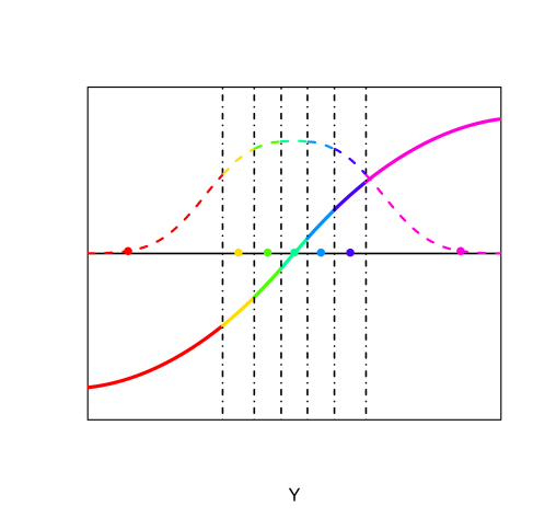
Figure 1: Below, with a solid line we plot the standardized inverse regression curve 𝔪(y):=sign(βj)𝔪j(y)Var(𝔪j(Y)),j𝒮𝜷formulae-sequenceassign𝔪𝑦signsubscript𝛽𝑗subscript𝔪𝑗𝑦Varsubscript𝔪𝑗𝑌𝑗subscript𝒮𝜷\mathfrak{m}(y):=\frac{\operatorname{sign}(\beta_{j})\mathfrak{m}_{j}(y)}{\sqrt{\operatorname{Var}(\mathfrak{m}_{j}(Y))}},j\in\mathcal{S}_{\boldsymbol{\beta}}, for the model Y=2atan(𝑿𝜷)+N(0,1)𝑌2atansuperscript𝑿𝜷𝑁01Y=2\operatorname{atan}(\boldsymbol{X}^{\intercal}\boldsymbol{\beta})+N(0,1) (see also (14)). The different colored parts of the dashed curve represent the conditional densities of Y|YShconditional𝑌𝑌subscript𝑆Y|Y\in S_{h}, where Shsubscript𝑆S_{h} for h[H]delimited-[]𝐻h\in[H] (with H = 777) are the slices illustrated by punctured vertical black lines. Finally the seven points’ vertical-axis values represent the variances Var[𝔪(Y)|YSh]Varconditional𝔪𝑌𝑌subscript𝑆\operatorname{Var}[\mathfrak{m}(Y)|Y\in S_{h}]. Sliced stability ensures that the average value of the variances Var[𝔪(Y)|YSh]Varconditional𝔪𝑌𝑌subscript𝑆\operatorname{Var}[\mathfrak{m}(Y)|Y\in S_{h}] has a decay rate of the order Hκ1superscript𝐻𝜅1H^{\kappa-1}.
Refer to caption

Definition 1 is the sliced stability definition from Lin et al. (2015) restated in terms of the SIM. Lin et al. (2015) conjectured that the sliced stability condition could be implied from the well accepted conditions proposed by Hsing & Carroll (1992), which we state below with a slight modification. The first contribution of this paper is proving this conjecture in the case of SIM.

Let 𝒜H(l,K)subscript𝒜𝐻𝑙𝐾\mathcal{A}_{H}(l,K), with 1<K,0<l<1formulae-sequence1𝐾0𝑙11<K,0<l<1, denote all partitions of \mathbb{R} of the sort {=a1a2aH+1=+\{-\infty=a_{1}\leq a_{2}\leq\ldots\leq a_{H+1}=+\infty}, such that lH(ahYah+1)KH𝑙𝐻subscript𝑎𝑌subscript𝑎1𝐾𝐻\frac{l}{H}\leq\mathbb{P}(a_{h}\leq Y\leq a_{h+1})\leq\frac{K}{H}. Moreover, for any fixed B𝐵B\in\mathbb{R}, let Πr(B)subscriptΠ𝑟𝐵\Pi_{r}(B) denote all possible partitions of the closed interval [B,B]𝐵𝐵[-B,B] into r𝑟r points Bb1b2brB𝐵subscript𝑏1subscript𝑏2subscript𝑏𝑟𝐵-B\leq b_{1}\leq b_{2}\leq\ldots\leq b_{r}\leq B. Define the normalized version of the centered inverse regression curve 𝔪(y):=sign(βj)𝔪j(y)Var(𝔪j(Y)),j[p]formulae-sequenceassign𝔪𝑦signsubscript𝛽𝑗subscript𝔪𝑗𝑦Varsubscript𝔪𝑗𝑌𝑗delimited-[]𝑝\mathfrak{m}(y):=\frac{\operatorname{sign}(\beta_{j})\mathfrak{m}_{j}(y)}{\sqrt{\operatorname{Var}(\mathfrak{m}_{j}(Y))}},j\in[p]222By symmetry sign(βj)𝔪j(y)=sign(βi)𝔪i(y)signsubscript𝛽𝑗subscript𝔪𝑗𝑦signsubscript𝛽𝑖subscript𝔪𝑖𝑦\operatorname{sign}(\beta_{j})\mathfrak{m}_{j}(y)=\operatorname{sign}(\beta_{i})\mathfrak{m}_{i}(y) for i,j𝒮𝜷𝑖𝑗subscript𝒮𝜷i,j\in\mathcal{S}_{\boldsymbol{\beta}}, and let 𝔪𝔪\mathfrak{m} satisfy the following smoothness condition:

limrsupbΠr(B)r1/(2+ξ)i=2r|𝔪(bi)𝔪(bi1)|=0,subscript𝑟subscriptsupremum𝑏subscriptΠ𝑟𝐵superscript𝑟12𝜉superscriptsubscript𝑖2𝑟𝔪subscript𝑏𝑖𝔪subscript𝑏𝑖10\displaystyle\lim_{r\rightarrow\infty}\sup_{b\in\Pi_{r}(B)}r^{-1/(2+\xi)}\sum_{i=2}^{r}|\mathfrak{m}(b_{i})-\mathfrak{m}(b_{i-1})|=0, (5)

for any B>0𝐵0B>0 for some fixed ξ>0𝜉0\xi>0. Note that as mentioned in Hsing & Carroll (1992), assumption (5) is weaker than assuming that 𝔪𝔪\mathfrak{m} is of bounded variation, and furthermore the bigger the ξ𝜉\xi the more stringent this assumption becomes. In addition, assume that there exists B0>0subscript𝐵00B_{0}>0 and a non-decreasing function 𝔪~:(B0,):~𝔪maps-tosubscript𝐵0\widetilde{\mathfrak{m}}:(B_{0},\infty)\mapsto\mathbb{R}, such that:

|𝔪(x)𝔪(y)||𝔪~(|x|)𝔪~(|y|)|, for x,y(,B0) or (B0,+),formulae-sequence𝔪𝑥𝔪𝑦~𝔪𝑥~𝔪𝑦 for 𝑥𝑦subscript𝐵0 or subscript𝐵0\displaystyle|\mathfrak{m}(x)-\mathfrak{m}(y)|\leq|\widetilde{\mathfrak{m}}(|x|)-\widetilde{\mathfrak{m}}(|y|)|,\mbox{ for }x,y\in(-\infty,-B_{0})\mbox{ or }(B_{0},+\infty), (6)

and moreover, 𝔼[|𝔪~(|Y|)|(2+ξ)]<𝔼delimited-[]superscript~𝔪𝑌2𝜉\mathbb{E}[|\widetilde{\mathfrak{m}}(|Y|)|^{(2+\xi)}]<\infty (where in the expectation we set 𝔪~(y)=0~𝔪𝑦0\widetilde{\mathfrak{m}}(y)=0 for |y|B0𝑦subscript𝐵0|y|\leq B_{0}). We are now in a position to formulate the following:

Proposition 1.

Assume that the standardized centered inverse regression curve satisfies properties (5) and (6) for some ξ>0𝜉0\xi>0. Then we have that for any fixed 0<l<1<K0𝑙1𝐾0<l<1<K:

limHsupa𝒜H(l,K)1H2/(2+ξ)h=1HVar[𝔪(Y)|ah<Yah+1]0.subscript𝐻subscriptsupremum𝑎subscript𝒜𝐻𝑙𝐾1superscript𝐻22𝜉superscriptsubscript1𝐻Varconditional𝔪𝑌subscript𝑎𝑌subscript𝑎10\displaystyle\lim_{H\rightarrow\infty}\sup_{a\in\mathcal{A}_{H}(l,K)}\frac{1}{H^{2/(2+\xi)}}\sum_{h=1}^{H}\operatorname{Var}[\mathfrak{m}(Y)|a_{h}<Y\leq a_{h+1}]\rightarrow 0. (7)

We defer the proof of Proposition 1 to Appendix A. It is clear however that (7) implies the existence of constants M𝑀M, C(l,K,M)𝐶𝑙𝐾𝑀C(l,K,M) such that (4) holds, with κ=22+ξ<1𝜅22𝜉1\kappa=\frac{2}{2+\xi}<1.

2.2 Optimal sample size for support recovery

Recall that Γ=nslog(ps)Γ𝑛𝑠𝑝𝑠\Gamma=\frac{n}{s\log(p-s)} is the rescaled sample size. First we establish an information theoretic barrier of the support recovery problem, i.e. we show that there exists a positive constant ω𝜔\omega such that, when Γ<ωΓ𝜔\Gamma<\omega every algorithm fails with probability at least 1/2121/2. Then we prove that two algorithms — DT-SIR and an SDP based procedure achieve this bound, i.e. we demonstrate that there exists a positive constant ΩΩ\Omega, such that, when Γ>ΩΓΩ\Gamma>\Omega, these two algorithms successfully recover the signed support with probability 111 as n𝑛n\rightarrow\infty.

2.2.1 Information theoretic barrier

Intuitively, when the sample size is small, no algorithm is expected to be able to recover the support successfully. In fact, let us consider the simple linear regression model:

Y=𝑿𝜷+ε where 𝑿Np(0,𝕀p),εN(0,σ2),formulae-sequence𝑌superscript𝑿𝜷𝜀 where 𝑿similar-tosubscript𝑁𝑝0subscript𝕀𝑝similar-to𝜀𝑁0superscript𝜎2\displaystyle Y=\boldsymbol{X}^{\intercal}\boldsymbol{\beta}+\varepsilon\mbox{ where }\boldsymbol{X}\sim N_{p}(0,\mathbb{I}_{p}),\varepsilon\sim N(0,\sigma^{2}), (8)

where 𝜷𝜷\boldsymbol{\beta} is a unit vector such that 𝜷i{±1s,0}subscript𝜷𝑖plus-or-minus1𝑠0\boldsymbol{\beta}_{i}\in\{\pm\frac{1}{\sqrt{s}},0\}. This model belongs to the class (σ2+1)1subscriptsuperscriptsuperscript𝜎211\mathcal{F}_{(\sigma^{2}+1)^{-1}} (to verify sliced stability refer to Example 2 and Remark 3 of Appendix B). The following result, which is obtained by a slight modification of the arguments in (Wainwright, 2009), shows that support recovery is infeasible if ΓΓ\Gamma is small, by effectively arguing that no algorithm works even for model (8).

Proposition 2.

Suppose there are n𝑛n observations from the model (8). Then there exists a positive constant ω𝜔\omega, such that if

Γ=nslog(ps)<ω,Γ𝑛𝑠𝑝𝑠𝜔\Gamma=\frac{n}{s\log(p-s)}<\omega,

any algorithm for support support recovery will have errors with probability at least 1212\frac{1}{2} asymptotically.

2.2.2 Optimality of DT-SIR

Recall that we are working with the class of models Asubscript𝐴\mathcal{F}_{A} (2). One key observation is the following signal strength result.

Lemma 1.

For any j 𝒮𝛃=supp(𝛃)absentsubscript𝒮𝛃𝑠𝑢𝑝𝑝𝛃\in\mathcal{S}_{\boldsymbol{\beta}}=supp(\boldsymbol{\beta}), one has:

AsVar(𝔪j(Y))1s,𝐴𝑠Varsubscript𝔪𝑗𝑌1𝑠\displaystyle\frac{A}{s}\leq\operatorname{Var}(\mathfrak{m}_{j}(Y))\leq\frac{1}{s}, (9)

and Var(𝔪j(Y))=0Varsubscript𝔪𝑗𝑌0\operatorname{Var}(\mathfrak{m}_{j}(Y))=0 for j𝒮𝛃𝑗subscript𝒮𝛃j\not\in\mathcal{S}_{\boldsymbol{\beta}}.

By Lemma 1 WLOG we can assume that there exists a CV>0subscript𝐶𝑉0C_{V}>0 such that Var[𝔪j(Y)]=CVsVarsubscript𝔪𝑗𝑌subscript𝐶𝑉𝑠\operatorname{Var}[\mathfrak{m}_{j}(Y)]=\frac{C_{V}}{s} for any j𝒮𝜷𝑗subscript𝒮𝜷j\in\mathcal{S}_{\boldsymbol{\beta}}. Now we are ready to discuss the properties of the DT algorithm which we formulate below. In this paper, we assume that the sparsity s𝑠s is known.

input : (Yi,𝑿i)i=1nsuperscriptsubscriptsubscript𝑌𝑖subscript𝑿𝑖𝑖1𝑛(Y_{i},\boldsymbol{X}_{i})_{i=1}^{n}: data, H𝐻H: number of slices, s𝑠s: the sparsity of 𝜷𝜷\boldsymbol{\beta}
  1. 1.

    Calcluate 𝐕jj,j[p]superscript𝐕𝑗𝑗𝑗delimited-[]𝑝\mathbf{V}^{jj},j\in[p] – according to formula (3);

  2. 2.

    Collect the s𝑠s highest 𝐕jjsuperscript𝐕𝑗𝑗\mathbf{V}^{jj} into the set S^^𝑆\widehat{S};

  3. 3.

    Output the set {j:𝐕jjS^}conditional-set𝑗superscript𝐕𝑗𝑗^𝑆\{j:\mathbf{V}^{jj}\in\widehat{S}\}.

Algorithm 1 DT algorithm

Recall the definitions (see (3)) of 𝐕𝐕\mathbf{V} and 𝐕jjsuperscript𝐕𝑗𝑗\mathbf{V}^{jj} the estimates of Cov[𝔼[𝑿|Y]]Cov𝔼delimited-[]conditional𝑿𝑌\operatorname{Cov}[\mathbb{E}[\boldsymbol{X}|Y]] and Var[𝔪j(Y)]Varsubscript𝔪𝑗𝑌\operatorname{Var}[\mathfrak{m}_{j}(Y)] respectively. To obtain the result on sample size optimality of Algorithm 1, a key point is to establish a concentration inequality for 𝐕jjsuperscript𝐕𝑗𝑗\mathbf{V}^{jj}. When j𝒮𝜷𝑗subscript𝒮𝜷j\not\in\mathcal{S}_{\boldsymbol{\beta}}, a standard deviation inequality for the χ2superscript𝜒2\chi^{2} distribution is applicable. For j𝒮𝜷𝑗subscript𝒮𝜷j\in\mathcal{S}_{\boldsymbol{\beta}}, we need to pay extra effort to obtain the appropriate deviation inequality, which is also the main technical contribution of this paper. Once we have established these deviation inequalities, we can show the following theorem.

Theorem 1.

Suppose s=O(p1δ)𝑠𝑂superscript𝑝1𝛿s=O(p^{1-\delta}) for some δ>0𝛿0\delta>0. There exists a positive constant ΩΩ\Omega such that, for any

Γ=nslog(ps)Ω,Γ𝑛𝑠𝑝𝑠Ω\displaystyle\Gamma=\frac{n}{s\log(p-s)}\geq\Omega, (10)

the support S𝑆S is recovered by the DT algorithm (i.e., S^=S^𝑆𝑆\widehat{S}=S) with probability converging to 111 as n𝑛n increases. Additionally, the number of slices can be held large enough but fixed (depending solely on C,l,K,M,κ,CV𝐶𝑙𝐾𝑀𝜅subscript𝐶𝑉C,l,K,M,\kappa,C_{V}).

Remark 1 (Choice of H𝐻H).

An interesting by-product of our analysis is that we can choose the number of slices H𝐻H large enough but finite. When dimension p𝑝p is fixed, this has already been observed in the literature (Li, 1991), however in high dimensional setting to the best of our knowledge this property has not been discussed.

Clearly the DT algorithm does not recover the signed support of 𝜷𝜷\boldsymbol{\beta} standalone. One can apply DT first to select the variables and then apply the SIR procedure to obtain an estimate of the principal eigenvector. To obtain the signed support of 𝜷𝜷\boldsymbol{\beta}, take the sign of the principal eigenvector. We summarize this algorithm in the following:

input : (Yi,𝑿i)i=1nsuperscriptsubscriptsubscript𝑌𝑖subscript𝑿𝑖𝑖1𝑛(Y_{i},\boldsymbol{X}_{i})_{i=1}^{n}: data, H𝐻H: number of slices, s𝑠s: the sparsity of 𝜷𝜷\boldsymbol{\beta}
  1. 1.

    Perform Algorithm 1 to obtain the set {j:𝐕jjS^}conditional-set𝑗superscript𝐕𝑗𝑗^𝑆\{j:\mathbf{V}^{jj}\in\widehat{S}\}.

  2. 2.

    Evaluate 𝐯𝐯{\mathbf{v}} — the principal eigenvector of the matrix 𝐕S^,S^subscript𝐕^𝑆^𝑆\mathbf{V}_{\widehat{S},\widehat{S}}.

  3. 3.

    Output sign(𝐯)sign𝐯\operatorname{sign}(\mathbf{v}).

Algorithm 2 DT-SIR

We note that this algorithm recovers the signed support, up to multiplication by ±1plus-or-minus1\pm 1. The following result is a direct corollary of Theorem 1, whose proof is omitted.

Proposition 3.

Under the assumptions of Theorem 1, with a potentially bigger value of ΩΩ\Omega, applying Algorithm 2 restores the signed support (up to a sign) with asymptotic probability converging to 111. In fact Algorithm 2 works when 𝐗Np(𝛍,𝕀p)similar-to𝐗subscript𝑁𝑝𝛍subscript𝕀𝑝\boldsymbol{X}\sim N_{p}(\boldsymbol{\mu},\mathbb{I}_{p}) with 𝐕𝐕\mathbf{V} substituted with 𝐕^^𝐕\widehat{\mathbf{V}} where the jk𝑗𝑘jkth entry of 𝐕^^𝐕\widehat{\mathbf{V}} is defined as 𝐕^jk=1Hh=1H(𝐗¯hj𝐗¯j)(𝐗¯hk𝐗¯k)superscript^𝐕𝑗𝑘1𝐻superscriptsubscript1𝐻subscriptsuperscript¯𝐗𝑗superscript¯𝐗𝑗subscriptsuperscript¯𝐗𝑘superscript¯𝐗𝑘\widehat{\mathbf{V}}^{jk}=\frac{1}{H}\sum_{h=1}^{H}(\overline{\boldsymbol{X}}^{j}_{h}-\overline{\boldsymbol{X}}^{j})(\overline{\boldsymbol{X}}^{k}_{h}-\overline{\boldsymbol{X}}^{k}).

2.2.3 Optimality of SDP

Algorithm 2 is a two-step procedure, selecting variables by applying DT and then obtaining the SIR estimate of 𝜷𝜷\boldsymbol{\beta}. Recent advances of optimization theory provide us with a more sophisticated one-step approach to obtain a sparse principal eigenvector. It is well known that the principal eigenvector of a symmetric positive definite matrix 𝐀𝐀\mathbf{A} is given by:

𝐳^=argmax𝐳:𝐳2=1𝐳𝐀𝐳^𝐳subscriptargmax:𝐳subscriptnorm𝐳21superscript𝐳𝐀𝐳\displaystyle\widehat{\mathbf{z}}=\operatornamewithlimits{argmax}_{\mathbf{z}\in\mathbb{R}:\|\mathbf{z}\|_{2}=1}\mathbf{z}^{\intercal}\mathbf{A}\mathbf{z}

and the principal eigenvalue is 𝐳^𝐀𝐳superscript^𝐳𝐀𝐳\widehat{\mathbf{z}}^{\intercal}\mathbf{A}\mathbf{z}. When 𝐳𝐳\mathbf{z} is sparse, i.e., 𝐳0ssubscriptnorm𝐳0𝑠\|\mathbf{z}\|_{0}\leq s , the above optimization problem with an additional sparsity constraint is computationally expensive. To remedy this difficulty, d’Aspremont et al. (2007) proposed an SDP approach to solve the sparse optimization problem. They suggested to solve the following convex program:

𝐙^=argmaxtr(𝐙)=1,𝐙𝕊+ptr(𝐀𝐙)λni,j=1p|𝐙ij|,^𝐙subscriptargmaxformulae-sequencetr𝐙1𝐙superscriptsubscript𝕊𝑝tr𝐀𝐙subscript𝜆𝑛superscriptsubscript𝑖𝑗1𝑝subscript𝐙𝑖𝑗\displaystyle\widehat{\mathbf{Z}}=\operatornamewithlimits{argmax}_{\operatorname{tr}(\mathbf{Z})=1,\mathbf{Z}\in\mathbb{S}_{+}^{p}}\operatorname{tr}(\mathbf{A}\mathbf{Z})-\lambda_{n}\sum_{i,j=1}^{p}|\mathbf{Z}_{ij}|, (11)

where 𝕊+psuperscriptsubscript𝕊𝑝\mathbb{S}_{+}^{p} is the set of all the p×p𝑝𝑝p\times p positive semi-definite matrices. If the solution happens to be a rank 1 solution, then it is of the form 𝐙^=𝐳^𝐳^^𝐙^𝐳superscript^𝐳\widehat{\mathbf{Z}}=\widehat{\mathbf{z}}\widehat{\mathbf{z}}^{\intercal}, and hence we can easily obtain an estimate of the principal eigenvector.

In the following algorithm we summarize the SDP approach, tailored for the signed support recovery of SIM. We remind the reader, that this algorithm recovers the signed support, up to multiplication by a global constant equal to ±1plus-or-minus1\pm 1.

input : (Yi,𝑿i)i=1nsuperscriptsubscriptsubscript𝑌𝑖subscript𝑿𝑖𝑖1𝑛(Y_{i},\boldsymbol{X}_{i})_{i=1}^{n}: data, H𝐻H: number of slices, s𝑠s: the sparsity of 𝜷𝜷\boldsymbol{\beta}
  1. 1.

    Calcluate the matrix 𝐕𝐕\mathbf{V} — as given in (3);

  2. 2.

    Obtain the matrix 𝐙^^𝐙\widehat{\mathbf{Z}} by solving (11), with 𝐀=𝐕𝐀𝐕\mathbf{A}=\mathbf{V};

  3. 3.

    Find the principal eigenvector 𝐳^^𝐳\widehat{\mathbf{z}} of 𝐙^^𝐙\widehat{\mathbf{Z}};

  4. 4.

    Output sign(𝐳^)sign^𝐳\operatorname{sign}(\widehat{\mathbf{z}}).

Algorithm 3 SDP algorithm for SIR

The performance of this algorithm is guaranteed by the following theorem.

Theorem 2.

Suppose s=O(p1δ)𝑠𝑂superscript𝑝1𝛿s=O(p^{1-\delta}) for some δ>0𝛿0\delta>0, then there is a positive constant ΩΩ\Omega such that, for any

Γ=nslog(ps)Ω,Γ𝑛𝑠𝑝𝑠Ω\displaystyle\Gamma=\frac{n}{s\log(p-s)}\geq\Omega, (12)

with a properly chosen the tuning parameter λnsubscript𝜆𝑛\lambda_{n} , Algorithm 3 recovers the signed support with probability converging to 1, i.e. (sign(𝐳^)=sign(𝛃))1sign^𝐳sign𝛃1\mathbb{P}(\operatorname{sign}(\widehat{\mathbf{z}})=\operatorname{sign}(\boldsymbol{\beta}))\rightarrow 1333We understand that 𝐳^^𝐳\widehat{\mathbf{z}} is selected so that 𝐳^𝛃0superscript^𝐳𝛃0\widehat{\mathbf{z}}^{\intercal}\boldsymbol{\beta}\geq 0 by convention..

Remark 2.

In fact Algorithm 3 works when 𝑿Np(𝝁,𝕀p)similar-to𝑿subscript𝑁𝑝𝝁subscript𝕀𝑝\boldsymbol{X}\sim N_{p}(\boldsymbol{\mu},\mathbb{I}_{p}) with 𝐕𝐕\mathbf{V} substituted with 𝐕^^𝐕\widehat{\mathbf{V}} where the jk𝑗𝑘jkth entry of 𝐕^^𝐕\widehat{\mathbf{V}} is defined as 𝐕^jk=1Hh=1H(𝑿¯hj𝑿¯j)(𝑿¯hk𝑿¯k)superscript^𝐕𝑗𝑘1𝐻superscriptsubscript1𝐻subscriptsuperscript¯𝑿𝑗superscript¯𝑿𝑗subscriptsuperscript¯𝑿𝑘superscript¯𝑿𝑘\widehat{\mathbf{V}}^{jk}=\frac{1}{H}\sum_{h=1}^{H}(\overline{\boldsymbol{X}}^{j}_{h}-\overline{\boldsymbol{X}}^{j})(\overline{\boldsymbol{X}}^{k}_{h}-\overline{\boldsymbol{X}}^{k}). The proof of this fact is trivial and is omitted.

3 Numerical Experiments and Data Analysis

We open this section with extensive numerical studies and in Section 3.2 we apply our algorithms to a real dataset.

3.1 Simulations

In this section we compare Algorithms 2 and 3 in terms of signed support recovery. We consider the following scenarios:

Y𝑌\displaystyle Y =𝑿𝜷+sin(𝑿𝜷)+N(0,1),absentsuperscript𝑿𝜷superscript𝑿𝜷𝑁01\displaystyle=\boldsymbol{X}^{\intercal}\boldsymbol{\beta}+\sin(\boldsymbol{X}^{\intercal}\boldsymbol{\beta})+N(0,1), (13)
Y𝑌\displaystyle Y =2atan(𝑿𝜷)+N(0,1),absent2atansuperscript𝑿𝜷𝑁01\displaystyle=2\operatorname{atan}(\boldsymbol{X}^{\intercal}\boldsymbol{\beta})+N(0,1), (14)
Y𝑌\displaystyle Y =(𝑿𝜷)3+N(0,1),absentsuperscriptsuperscript𝑿𝜷3𝑁01\displaystyle=(\boldsymbol{X}^{\intercal}\boldsymbol{\beta})^{3}+N(0,1), (15)
Y𝑌\displaystyle Y =sinh(𝑿𝜷)+N(0,1).absentsinhsuperscript𝑿𝜷𝑁01\displaystyle=\operatorname{sinh}(\boldsymbol{X}^{\intercal}\boldsymbol{\beta})+N(0,1). (16)

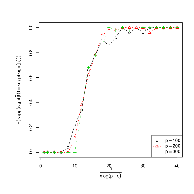
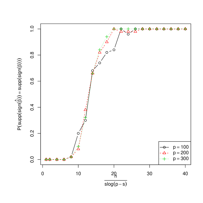
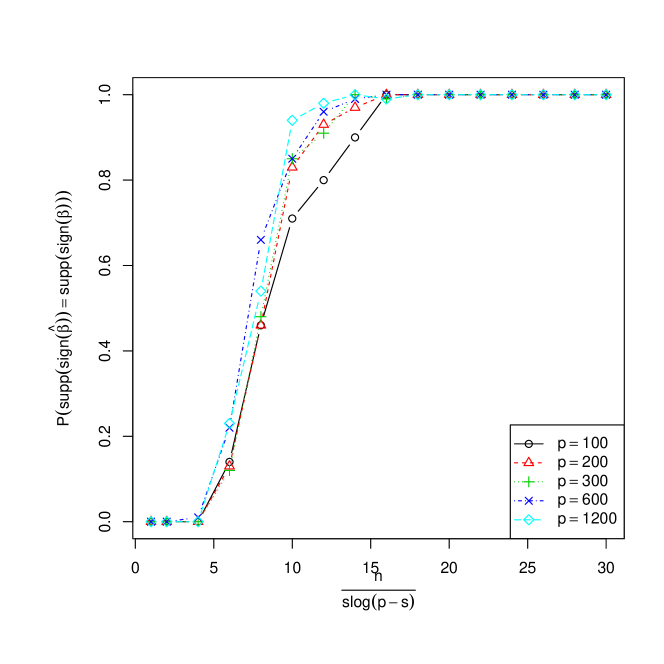
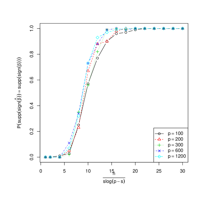
In each simulation we create a sample of size n𝑛n with dimensionality p𝑝p and sparsity levels s=p𝑠𝑝s=\sqrt{p} (s=log(p)𝑠𝑝s=\log(p) resp.) and we vary the rescaled sample size Γ[0,30]Γ030\Gamma\in[0,30] for the DT-SIR and Γ[0,40]Γ040\Gamma\in[0,40] for the SDP approach. The vector 𝜷𝜷\boldsymbol{\beta} is selected in the following manner:

βj=1s,j[s1],βs=1s, and βj=0, for j>s.formulae-sequencesubscript𝛽𝑗1𝑠formulae-sequence𝑗delimited-[]𝑠1formulae-sequencesubscript𝛽𝑠1𝑠formulae-sequence and subscript𝛽𝑗0 for 𝑗𝑠\beta_{j}=\frac{1}{\sqrt{s}},~{}j\in[s-1],~{}~{}\beta_{s}=-\frac{1}{\sqrt{s}},\mbox{ and }\beta_{j}=0,\mbox{ for }j>s.

Each simulation is repeated 500500500 times, and we report the proportion of correctly recovered signed supports of the vector 𝜷𝜷\boldsymbol{\beta}. We remark that in general, it should not be expected that the phase transition described in Theorems 1 and 2 to occur at the same places for these 444 models.

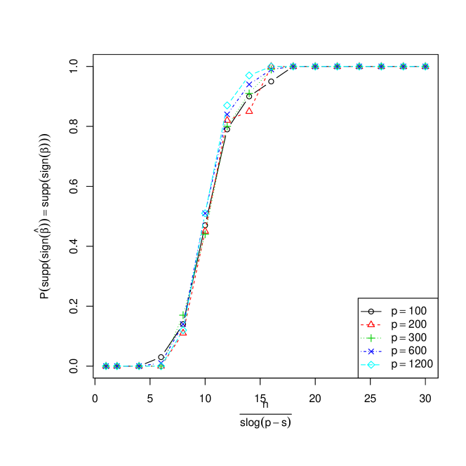
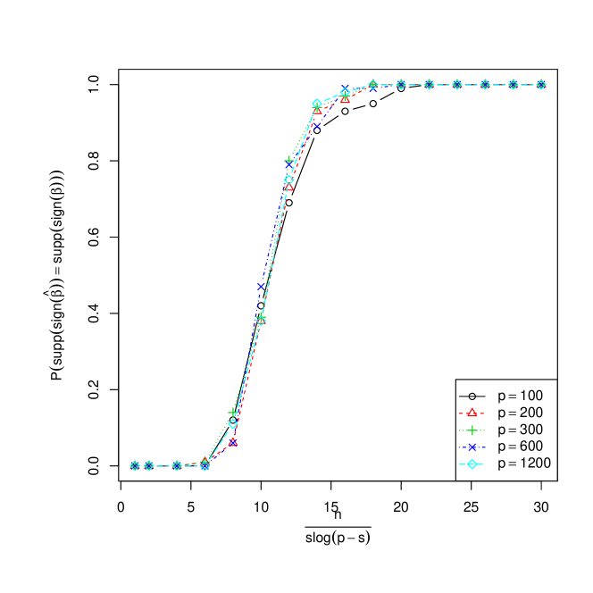
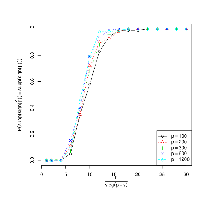
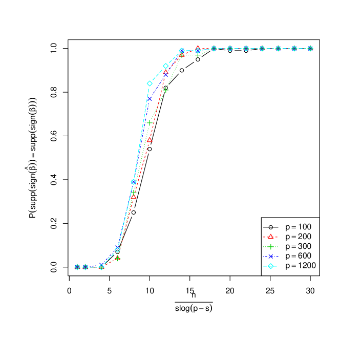
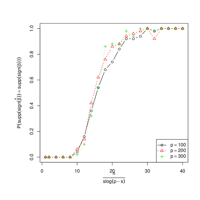
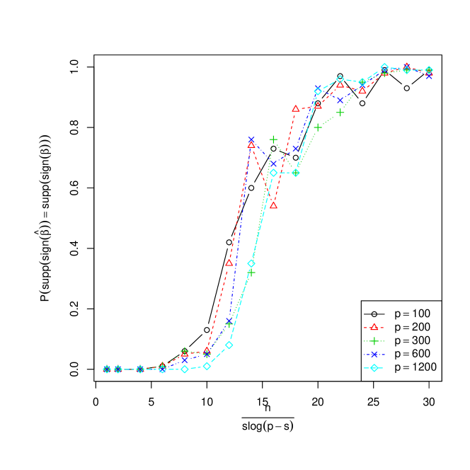
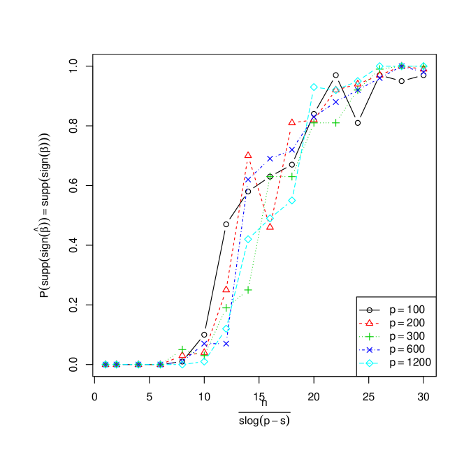
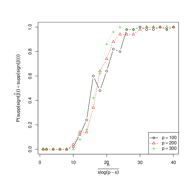
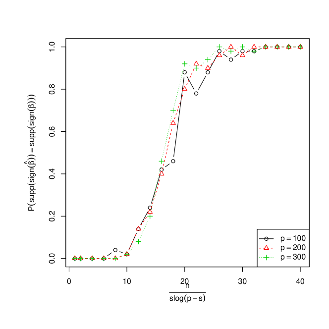
We first explore the predictions of Proposition 3 and Algorithm 2. Even though we provide theoretical values of the constants H𝐻H and m𝑚m, we ran all simulations with H=10𝐻10H=10 slices. We believe this scenario, is still reflective of the true nature of the DT-SIR algorithm, as the theoretical value of H𝐻H we provide is not optimized in any fashion. In Figure 2, we present DT-SIR results from plots for different p𝑝p values in the regime s=p𝑠𝑝s=\sqrt{p}.

Figure 2: Efficiency Curves for DT-SIR, s=p,Γ=nslog(ps)[0,30]formulae-sequence𝑠𝑝Γ𝑛𝑠𝑝𝑠030s=\sqrt{p},~{}\Gamma=\frac{n}{s\log(p-s)}\in[0,30]
Refer to caption
(a) Model (13)
Refer to caption
(b) Model (14)
Refer to caption
(c) Model (15)
Refer to caption
(d) Model (16)

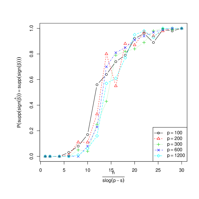
On the X𝑋X-axis we have plotted the rescaled sample size nslog(ps)𝑛𝑠𝑝𝑠\frac{n}{s\log(p-s)} and on the Y𝑌Y-axis is the estimated probability of successful signed support recovery. We would refer to these curves as efficiency curves (EC). The EC plots in the case s=p𝑠𝑝s=\sqrt{p}, are very similar to the corresponding plots in the regime s=log(p)𝑠𝑝s=\log(p), which can be seen in Figure 4 in Appendix C. Both EC plots are in concordance with the predictions from our theoretical results. We can distinctly see the phase transition occurring in approximately the same place regardless of the values of the dimension p𝑝p.

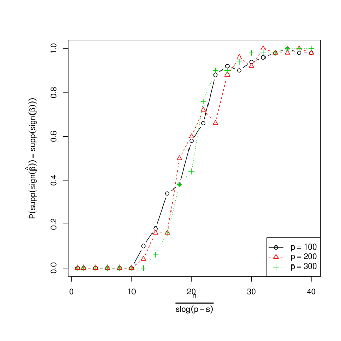
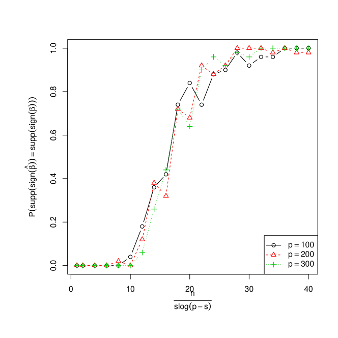
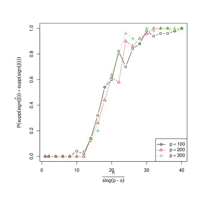
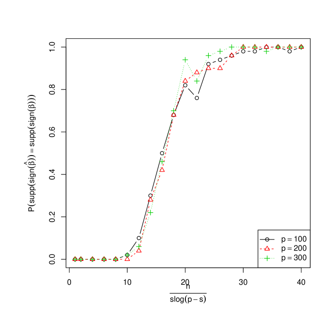
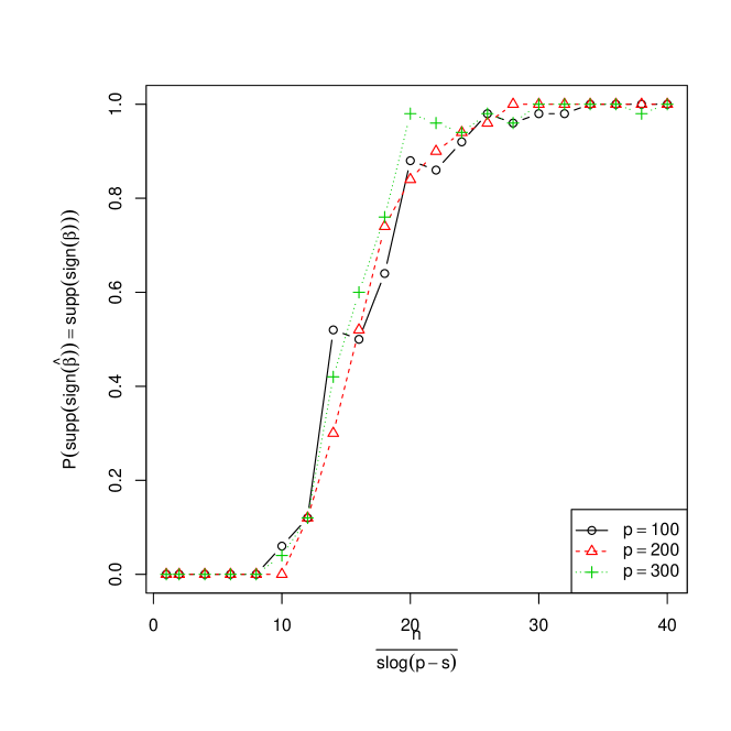
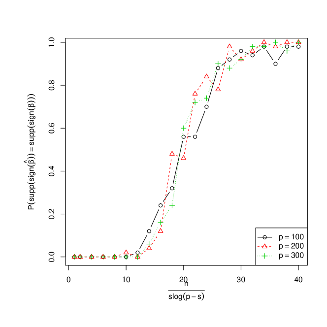
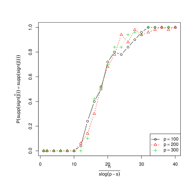
Next, we present the corresponding ECs for Algorithm 3. We used the code from an efficient implementation of program (11), as suggested in Zhang & Ghaoui (2011). The code was kindly provided to us by the authors of Zhang & Ghaoui (2011). In Figure 3 we plot the ECs for the four models in the case when s=p𝑠𝑝s=\sqrt{p}. Due to running time limitations we only show scenarios where p{100,200,300}𝑝100200300p\in\{100,200,300\}.

Figure 3: Efficiency Curves for SDP, s=p,Γ=nslog(ps)[0,40]formulae-sequence𝑠𝑝Γ𝑛𝑠𝑝𝑠040s=\sqrt{p},~{}\Gamma=\frac{n}{s\log(p-s)}\in[0,40]
Refer to caption
(a) Model (13)
Refer to caption
(b) Model (14)
Refer to caption
(c) Model (15)
Refer to caption
(d) Model (16)

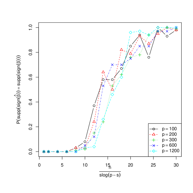
Here we have again used H=10𝐻10H=10 in all scenarios, for simplicity. We observe that phase transitions are occurring in all of the models, and the signed support is being correctly recovered for large enough values of Γ=nslog(ps)Γ𝑛𝑠𝑝𝑠\Gamma=\frac{n}{s\log(p-s)}. Plots for the setting s=log(p)𝑠𝑝s=\log(p) are provided in Figure 5. An important empirical observation is that the constant ΩΩ\Omega needs to be higher when running the SDP algorithm compared to when running the DT-SIR. This fact coupled with the much slower run-times of the SDP algorithm speak in favor of using the DT-SIR algorithm in practice.

In addition to the above simulations, we also performed numerical studies over the same set of models (13), (14), (15) and (16), where the coefficients of the vector 𝜷𝜷\boldsymbol{\beta} were not of equal magnitude. In our second set of simulations we chose 𝜷=𝜷~𝜷~2𝜷~𝜷subscriptnorm~𝜷2\boldsymbol{\beta}=\frac{\widetilde{\boldsymbol{\beta}}}{\|\widetilde{\boldsymbol{\beta}}\|_{2}}, where the entries of 𝜷~~𝜷\widetilde{\boldsymbol{\beta}} were drawn in each simulation as

β~j=Uj for js/2,β~j=Uj for s/2<js, and β~j=0 otherwise,formulae-sequencesubscript~𝛽𝑗subscript𝑈𝑗 for 𝑗𝑠2subscript~𝛽𝑗subscript𝑈𝑗 for 𝑠2𝑗𝑠 and subscript~𝛽𝑗0 otherwise,\displaystyle\tilde{\beta}_{j}=U_{j}\mbox{ for }j\leq\lfloor s/2\rfloor,~{}~{}\tilde{\beta}_{j}=-U_{j}\mbox{ for }s/2<j\leq s,\mbox{ and }\tilde{\beta}_{j}=0\mbox{ otherwise,} (17)

where Ujsubscript𝑈𝑗U_{j} for j[s]𝑗delimited-[]𝑠j\in[s] are i.i.d. uniform U(12,1)𝑈121U(\frac{1}{2},1) random variables. The results are similar to the ones reported above, although the efficiency curves required somewhat higher values of the rescaled sample size ΓΓ\Gamma, and extra variability can be seen in the curves due to the random choice of 𝜷𝜷\boldsymbol{\beta}. This is to be expected, since under such a generation scheme, the lowest signal will be of lower magnitude compared to the uniform signal case. We show the results for the case s=p𝑠𝑝s=\sqrt{p} in Appendix C under Figures 6 and 7. Due to space considerations, we do not show results for the case s=logp𝑠𝑝s=\log p, as the results are comparable to the results plotted in Figures 4 and 5.

3.2 Real Data Example

In this sub-section we will illustrate the practical benefits of our algorithm on a real dataset. Our dataset is the mouse embryonic stem cells (ESCs) dataset, and has been previously analyzed by Zhong et al. (2012); Jiang et al. (2014).

The outcome variable is the expression levels of 12,4081240812,408 genes, and is derived using RNA-seq technology in mouse ESCs (Cloonan et al., 2008). The predictors correspond to 312312312 transcription factors (TFs). From the predictors, 121212 TFs are known to be associated with different roles in the ES-cell biology as constituents of important signaling pathways, self renewal regulators, and key reprogramming factors, and the remaining 300300300 are putative mouse TFs compiled from the TRANSFAC database. For each gene and TF, the predictor matrix contains a score which is the transcription factor association strength score (Chen et al., 2008; Ouyang et al., 2009) for the 121212 known TFs, and motif matching scores for the remaining 300300300 genes which were introduced by Zhong et al. (2012). Hence, the design matrix 𝕏=(𝑿i)i[n]𝕏subscriptsuperscriptsuperscriptsubscript𝑿𝑖𝑖delimited-[]𝑛\mathbb{X}=(\boldsymbol{X}_{i}^{\intercal})^{\intercal}_{i\in[n]} is a n×p𝑛𝑝n\times p matrix, where n=12,408𝑛12408n=12,408 and p=312𝑝312p=312, each entry of which represents the score of a TF for the corresponding gene. The EFCs dataset is not truly a high-dimensional dataset in the sense n<p𝑛𝑝n<p, but serves to illustrate that our algorithms can successfully perform variable selection. Since 𝕏𝕏\mathbb{X} is coming from a real dataset with non-homogeneous scores across the predictors, we wouldn’t expect it to be centered with identity covariance. To deal with this problem we use the statistics 𝐕~jksubscript~𝐕𝑗𝑘\widetilde{\mathbf{V}}_{jk} in place of 𝐕jksubscript𝐕𝑗𝑘\mathbf{V}_{jk} where the matrix 𝐕~~𝐕\widetilde{\mathbf{V}} is defined as:

𝐕~:=𝚺^1/21Hh=1H(𝑿¯h𝑿¯)(𝑿¯h𝑿¯)𝚺^1/2,assign~𝐕superscript^𝚺121𝐻superscriptsubscript1𝐻subscript¯𝑿¯𝑿superscriptsubscript¯𝑿¯𝑿superscript^𝚺12\widetilde{\mathbf{V}}:=\widehat{\boldsymbol{\Sigma}}^{-1/2}\frac{1}{H}\sum_{h=1}^{H}(\overline{\boldsymbol{X}}_{h}-\overline{\boldsymbol{X}})(\overline{\boldsymbol{X}}_{h}-\overline{\boldsymbol{X}})^{\intercal}\widehat{\boldsymbol{\Sigma}}^{-1/2},

and 𝚺^1/2:=[n1i[n](𝑿i𝑿¯)(𝑿i𝑿¯)]1/2assignsuperscript^𝚺12superscriptdelimited-[]superscript𝑛1subscript𝑖delimited-[]𝑛subscript𝑿𝑖¯𝑿superscriptsubscript𝑿𝑖¯𝑿12\widehat{\boldsymbol{\Sigma}}^{-1/2}:=\Big{[}n^{-1}\sum_{i\in[n]}(\boldsymbol{X}_{i}-\overline{\boldsymbol{X}})(\boldsymbol{X}_{i}-\overline{\boldsymbol{X}})^{\intercal}\Big{]}^{-1/2} is the symmetric square root of the covariance matrix of 𝕏𝕏\mathbb{X}. Notice that in this dataset 𝚺^1/2superscript^𝚺12\widehat{\boldsymbol{\Sigma}}^{-1/2} can be estimated without the application of sparse inverse procedures since n>p𝑛𝑝n>p. As in the simulation section we used H=10𝐻10H=10 slices.

We ran the DT and SDP procedures (i.e. Algorithms 1 and 3) on the ESCs dataset, and the DT procedure selected 282828 TFs which it found associated with the outcome, while the SDP procedure selected 363636. In Table 1 we compare the rankings of the 121212 known ES-cell TFs within the TFs selected by DT and SDP algorithms to the same rankings produced by the procedures SIRI-AE (Jiang et al., 2014) and COP (Zhong et al., 2012).

Table 1: Rankings of the 121212 known TFs among the selected TFs by different algorithms
TFs names DT SDP SIRI-AE COP
E2f1 1 1 1 1
Zfx 2 3 3 3
Mycn 3 2 4 10
Klf4 7 4 5 19
Myc 4 7 6
Esrrb 14 10 8
Oct4 20 20 9 11
Tcfcp2l1 8 8 10 36
Nanog 11 17 14
Stat3 23 17 20
Sox2 24 18
Smad1 25 25 32 13

The top 101010 highly ranked genes of SIRI-AE, DT, SDP and COP contain 8,6,7,386738,6,7,3 known ES-cell TFs respectively. The DT algorithm is the most parsimonious out of all procedures (SIRI-AE and COP have reportedly selected 343434 and 424242 TFs correspondingly), but nevertheless includes all of the known TFs with the exception of the Stat3. The DT algorithm is additionally able to capture both Nanog and Sox2 which are generally believed to be the master ESC regulators. These TFs are completely missed by COP and the Sox2 TF was omitted by SDP. The SIRI-AE algorithm is the only algorithm which is able to recognize all of the 121212 known TFs. We would like to mention that compared to our work the SIRI-AE algorithm is designed to work in a lower dimensional setup, and is able to capture interactions beyond the single-index models, which could help explain its better performance on the ESCs dataset.

All in all, we believe the results of our algorithms are satisfactory, and illustrate that both DT and SDP can be successfully applied in practice. As a remark, in a truly high-dimensional setting when n<p𝑛𝑝n<p, instead of the estimate 𝚺^1/2superscript^𝚺12\widehat{\boldsymbol{\Sigma}}^{-1/2}, in practice one might resort to sparse estimators produced by procedures such as CLIME (Cai et al., 2011), and use the corrected statistics 𝐕~~𝐕\widetilde{\mathbf{V}} in place of 𝐕𝐕\mathbf{V}.

4 Proof of Theorem 1

We will prove this theorem under slightly more general conditions:

  • i.

    Let 𝑿jsuperscript𝑿𝑗\boldsymbol{X}^{j}, j[p]𝑗delimited-[]𝑝j\in[p] be centered, sub-Gaussian random variables with maxj[p]𝑿jψ2𝒦subscript𝑗delimited-[]𝑝subscriptnormsuperscript𝑿𝑗subscript𝜓2𝒦\max_{j\in[p]}\|\boldsymbol{X}^{j}\|_{\psi_{2}}\leq\mathcal{K}.

  • ii.

    For j𝒮𝜷𝑗subscript𝒮𝜷j\in\mathcal{S}_{\boldsymbol{\beta}}, we assume that Var[𝔪j(Y)]CVsVardelimited-[]subscript𝔪𝑗𝑌subscript𝐶𝑉𝑠\mathrm{Var}[\mathfrak{m}_{j}(Y)]\geq\frac{C_{V}}{s}.

  • iii.

    For j𝒮𝜷c𝑗subscriptsuperscript𝒮𝑐𝜷j\in\mathcal{S}^{c}_{\boldsymbol{\beta}}, we assume that 𝔪j(Y)=𝔼[𝑿j|Y]=0subscript𝔪𝑗𝑌𝔼delimited-[]conditionalsuperscript𝑿𝑗𝑌0\mathfrak{m}_{j}(Y)=\mathbb{E}[\boldsymbol{X}^{j}|Y]=0 a.s.

It is easy to see for that for SIM in Asubscript𝐴\mathcal{F}_{A}, the above conditions are satisfied in the case when 𝑿Np(0,𝕀p)similar-to𝑿subscript𝑁𝑝0subscript𝕀𝑝\boldsymbol{X}\sim N_{p}(0,\mathbb{I}_{p}). We start with a high level outline of the proof. As we pointed out, the key argument is to show a deviation inequality for 𝐕jjsuperscript𝐕𝑗𝑗\mathbf{V}^{jj}, i.e. we will show that |𝐕jjVar[𝔪j(Y)]|superscript𝐕𝑗𝑗Varsubscript𝔪𝑗𝑌|\mathbf{V}^{jj}-\operatorname{Var}[\mathfrak{m}_{j}(Y)]| is small (e.g. <13Var[𝔪j(Y)]absent13Varsubscript𝔪𝑗𝑌<\frac{1}{3}\operatorname{Var}[\mathfrak{m}_{j}(Y)]) with high probability provided that Γ=nslog(ps)Γ𝑛𝑠𝑝𝑠\Gamma=\frac{n}{s\log(p-s)} is large enough. Note that:

|𝐕jjVar[𝔪j(Y)]|superscript𝐕𝑗𝑗Varsubscript𝔪𝑗𝑌\displaystyle|\mathbf{V}^{jj}-\operatorname{Var}[\mathfrak{m}_{j}(Y)]| =|1Hh=1H(𝑿¯hj)2𝔪j2(y)pY(y)𝑑y|.absent1𝐻superscriptsubscript1𝐻superscriptsuperscriptsubscript¯𝑿𝑗2subscriptsuperscript𝔪2𝑗𝑦subscript𝑝𝑌𝑦differential-d𝑦\displaystyle=\left|\frac{1}{H}\sum_{h=1}^{H}\left(\overline{\boldsymbol{X}}_{h}^{j}\right)^{2}-\int\mathfrak{m}^{2}_{j}(y)p_{Y}(y)dy\right|. (18)

We will show below (see (22)), that the above expression is well approximated by:

|1Hh=1H(𝑿¯hj)2h=1H(𝝁hj)2(YSh)|,1𝐻superscriptsubscript1𝐻superscriptsuperscriptsubscript¯𝑿𝑗2superscriptsubscript1𝐻superscriptsubscriptsuperscript𝝁𝑗2𝑌subscript𝑆\displaystyle\left|\frac{1}{H}\sum_{h=1}^{H}\left(\overline{\boldsymbol{X}}_{h}^{j}\right)^{2}-\sum_{h=1}^{H}(\boldsymbol{\mu}^{j}_{h})^{2}\mathbb{P}(Y\in S_{h})\right|, (19)

under sliced stability (where Y(0)=subscript𝑌0Y_{(0)}=-\infty). Intuitively, we have 1) (YSh)1H𝑌subscript𝑆1𝐻\mathbb{P}(Y\in S_{h})\approx\frac{1}{H} and 2) 𝑿¯hj𝝁hjsubscriptsuperscript¯𝑿𝑗superscriptsubscript𝝁𝑗\overline{\boldsymbol{X}}^{j}_{h}\approx\boldsymbol{\mu}_{h}^{j}, which shows that (19) should be close to 0. To rigorously validate this intuition, we use the Dvoretzky-Kiefer-Wolfowitz (DKW) inequality (Massart, 1990) for 1) and concentration inequalities for 2).

Note that the probability (YSh)𝑌subscript𝑆\mathbb{P}(Y\in S_{h}) is a random variable, where the randomness comes from the two endpoints — Y(m(h1))subscript𝑌𝑚1Y_{(m(h-1))} and Y(mh)subscript𝑌𝑚Y_{(mh)} of the interval Shsubscript𝑆S_{h}. Recall that Fnsubscript𝐹𝑛F_{n} is the empirical distribution function of Y𝑌Y, based on the sample Yisubscript𝑌𝑖Y_{i}. By the DKW inequality, we have that (supy|Fn(y)F(y)|>ϵ)2exp(2nϵ2)subscriptsupremum𝑦subscript𝐹𝑛𝑦𝐹𝑦italic-ϵ22𝑛superscriptitalic-ϵ2\mathbb{P}(\sup_{y}|F_{n}(y)-F(y)|>\epsilon)\leq 2\exp(-2n\epsilon^{2}), which in addition to the fact that Y𝑌Y has a continuous distribution, implies that for all hh we have:

1H2ϵ(h1H<Fn(Y)<hH)(h1HFn(Y)hH)1H+2ϵ,1𝐻2italic-ϵ1𝐻subscript𝐹𝑛𝑌𝐻1𝐻subscript𝐹𝑛𝑌𝐻1𝐻2italic-ϵ\displaystyle\frac{1}{H}-2\epsilon\leq\mathbb{P}\left(\frac{h-1}{H}<F_{n}(Y)<\frac{h}{H}\right)\leq\mathbb{P}\left(\frac{h-1}{H}\leq F_{n}(Y)\leq\frac{h}{H}\right)\leq\frac{1}{H}+2\epsilon, (20)

on an event with probability at least 12exp(2nϵ2)122𝑛superscriptitalic-ϵ21-2\exp(-2n\epsilon^{2}). Denote the event where (20) holds with E𝐸E.

Next, notice that for h[H2]delimited-[]𝐻2h\in[H-2] and a random permutation π:[m1][m1]:𝜋maps-todelimited-[]𝑚1delimited-[]𝑚1\pi:[m-1]\mapsto[m-1], the collection random variables 𝑿h,πij,i[m1]subscriptsuperscript𝑿𝑗subscript𝜋𝑖𝑖delimited-[]𝑚1\boldsymbol{X}^{j}_{h,\pi_{i}},i\in[m-1] are conditionally i.i.d. given (Y(m(h1)),Y(mh))subscript𝑌𝑚1subscript𝑌𝑚(Y_{(m(h-1))},Y_{(mh)}), and for h=H1𝐻1h=H-1 and a random permutation π:[m][m]:𝜋maps-todelimited-[]𝑚delimited-[]𝑚\pi:[m]\mapsto[m] the random variables 𝑿h,πij,i[m]subscriptsuperscript𝑿𝑗subscript𝜋𝑖𝑖delimited-[]𝑚\boldsymbol{X}^{j}_{h,\pi_{i}},i\in[m] are conditionally i.i.d. given Y(m(H1))subscript𝑌𝑚𝐻1Y_{(m(H-1))}, as they can be generated via simple rejection sampling. Hence conditionally on (Y(mh))h[H1]subscriptsubscript𝑌𝑚delimited-[]𝐻1(Y_{(mh)})_{h\in[H-1]} the sample means 𝑿¯h,1:(m1)jsubscriptsuperscript¯𝑿𝑗:1𝑚1\overline{\boldsymbol{X}}^{j}_{h,1:(m-1)} have corresponding means 𝝁hjsubscriptsuperscript𝝁𝑗\boldsymbol{\mu}^{j}_{h} when h[H1]delimited-[]𝐻1h\in[H-1] and 𝑿¯Hjsubscriptsuperscript¯𝑿𝑗𝐻\overline{\boldsymbol{X}}^{j}_{H} has a mean of 𝝁Hjsubscriptsuperscript𝝁𝑗𝐻\boldsymbol{\mu}^{j}_{H}. For consistency of notation we will discard a point at random in the H𝐻Hth slice, and WLOG (upon re-labeling the points) we assume that the discarded point is 𝑿H,msubscript𝑿𝐻𝑚\boldsymbol{X}_{H,m}. Next, we formulate the following concentration result for the sliced means, which we show in Appendix A:

Lemma 2.

Let G[p]𝐺delimited-[]𝑝G\subseteq[p]. On the event E𝐸E, for η>0𝜂0\eta>0 we have the following:

(maxjG,h[H]|𝑿¯h,1:(m1)j𝝁hj|>η)2|G|Hexp(η2(m1)C1𝒦2q1+C2𝒦η),subscriptformulae-sequence𝑗𝐺delimited-[]𝐻superscriptsubscript¯𝑿:1𝑚1𝑗superscriptsubscript𝝁𝑗𝜂2𝐺𝐻superscript𝜂2𝑚1subscript𝐶1superscript𝒦2superscript𝑞1subscript𝐶2𝒦𝜂\displaystyle\mathbb{P}\left(\max_{j\in G,h\in[H]}\left|\overline{\boldsymbol{X}}_{h,1:(m-1)}^{j}-\boldsymbol{\mu}_{h}^{j}\right|>\eta\right)\leq 2|G|H\exp\left(-\frac{\eta^{2}(m-1)}{C_{1}\mathcal{K}^{2}q^{-1}+C_{2}\mathcal{K}\eta}\right), (21)

where q=1H2ϵ𝑞1𝐻2italic-ϵq=\frac{1}{H}-2\epsilon, for some absolute constants C1,C2>0subscript𝐶1subscript𝐶20C_{1},C_{2}>0.

Set G=[p]𝐺delimited-[]𝑝G=[p] and denote with E~~𝐸\widetilde{E} the event on which we have

maxj[p],h[H]|𝑿¯h,1:(m1)j𝝁hj|η.subscriptformulae-sequence𝑗delimited-[]𝑝delimited-[]𝐻superscriptsubscript¯𝑿:1𝑚1𝑗superscriptsubscript𝝁𝑗𝜂\max_{j\in[p],h\in[H]}\left|\overline{\boldsymbol{X}}_{h,1:(m-1)}^{j}-\boldsymbol{\mu}_{h}^{j}\right|\leq\eta.

By (21), (20) and the union bound we have that:

(E~)~𝐸\displaystyle\mathbb{P}(\widetilde{E}) 12pHexp(η2(m1)C1𝒦2q1+C2𝒦η)2exp(2nϵ2).absent12𝑝𝐻superscript𝜂2𝑚1subscript𝐶1superscript𝒦2superscript𝑞1subscript𝐶2𝒦𝜂22𝑛superscriptitalic-ϵ2\displaystyle\geq 1-2pH\exp\left(-\frac{\eta^{2}(m-1)}{C_{1}\mathcal{K}^{2}q^{-1}+C_{2}\mathcal{K}\eta}\right)-2\exp(-2n\epsilon^{2}).

Next we move on, to show that (18) is close to (19) on the event E𝐸E, as well as we collect two straightforward inequalities in the following helpful:

Lemma 3.

Assume that the sliced stability condition (4) holds. Then we have the following inequalities holding on the event E𝐸E, for large enough H𝐻H, and small enough ϵitalic-ϵ\epsilon:

|𝐕jjVar[𝔪j(Y)]|superscript𝐕𝑗𝑗Varsubscript𝔪𝑗𝑌\displaystyle|\mathbf{V}^{jj}-\operatorname{Var}[\mathfrak{m}_{j}(Y)]| |1Hh=1H(𝑿¯hj)2h=1H(𝝁hj)2(YSh)|absent1𝐻superscriptsubscript1𝐻superscriptsuperscriptsubscript¯𝑿𝑗2superscriptsubscript1𝐻superscriptsubscriptsuperscript𝝁𝑗2𝑌subscript𝑆\displaystyle\leq\left|\frac{1}{H}\sum_{h=1}^{H}\left(\overline{\boldsymbol{X}}_{h}^{j}\right)^{2}-\sum_{h=1}^{H}(\boldsymbol{\mu}^{j}_{h})^{2}\mathbb{P}(Y\in S_{h})\right| (22)
+CHκs(1H+2ϵ)B1,subscript𝐶superscript𝐻𝜅𝑠1𝐻2italic-ϵsubscript𝐵1\displaystyle+\underbrace{\frac{CH^{\kappa}}{s}\left(\frac{1}{H}+2\epsilon\right)}_{B_{1}},
h=1H(𝝁hj)2superscriptsubscript1𝐻superscriptsuperscriptsubscript𝝁𝑗2\displaystyle\sum_{h=1}^{H}(\boldsymbol{\mu}_{h}^{j})^{2} CVs+B1(1H2ϵ)B2,absentsubscriptsubscript𝐶𝑉𝑠subscript𝐵11𝐻2italic-ϵsubscript𝐵2\displaystyle\leq\underbrace{\frac{\frac{C_{V}}{s}+B_{1}}{\left(\frac{1}{H}-2\epsilon\right)}}_{B_{2}}, (23)
h=1H|𝝁hj|superscriptsubscript1𝐻superscriptsubscript𝝁𝑗\displaystyle\sum_{h=1}^{H}|\boldsymbol{\mu}_{h}^{j}| CVs+B1(1H2ϵ)B3.absentsubscriptsubscript𝐶𝑉𝑠subscript𝐵11𝐻2italic-ϵsubscript𝐵3\displaystyle\leq\underbrace{\frac{\sqrt{\frac{C_{V}}{s}+B_{1}}}{\left(\frac{1}{H}-2\epsilon\right)}}_{B_{3}}. (24)

Note. We refer to the constants from (4) as C𝐶C and κ𝜅\kappa, dropping the dependence on K𝐾K and M𝑀M for brevity, and in fact C=C(l,K,M)CV𝐶𝐶𝑙𝐾𝑀subscript𝐶𝑉C=C(l,K,M)C_{V}.

Note that by an elementary calculation — using (20) and Lemma 3, on the event E~~𝐸\widetilde{E} we get:

|𝐕jjVar[𝔪j(Y)]|superscript𝐕𝑗𝑗Varsubscript𝔪𝑗𝑌\displaystyle|\mathbf{V}^{jj}-\operatorname{Var}[\mathfrak{m}_{j}(Y)]| 1Hh=1H|(𝑿¯hj)2(m1)2m2(𝝁hj)2|absent1𝐻superscriptsubscript1𝐻superscriptsuperscriptsubscript¯𝑿𝑗2superscript𝑚12superscript𝑚2superscriptsuperscriptsubscript𝝁𝑗2\displaystyle\leq\frac{1}{H}\sum_{h=1}^{H}\left|\left(\overline{\boldsymbol{X}}_{h}^{j}\right)^{2}-\frac{(m-1)^{2}}{m^{2}}(\boldsymbol{\mu}_{h}^{j})^{2}\right| (25)
+(2ϵ+1H(m1)2Hm2)B2I1+B1I2,subscript2italic-ϵ1𝐻superscript𝑚12𝐻superscript𝑚2subscript𝐵2subscript𝐼1subscriptsubscript𝐵1subscript𝐼2\displaystyle+\underbrace{\left(2\epsilon+\frac{1}{H}-\frac{(m-1)^{2}}{Hm^{2}}\right)B_{2}}_{I_{1}}+\underbrace{B_{1}}_{I_{2}}, (26)

where we used (22), the triangle inequality and (23). Consider the following:

Lemma 4.

There exists a subset E~~E~~~𝐸~𝐸\widetilde{\widetilde{E\,}}\subset\widetilde{E} such that (E~E~~)pexp(cτ2n4𝒦4)~𝐸~~𝐸𝑝𝑐superscript𝜏2𝑛4superscript𝒦4\mathbb{P}({\widetilde{E}\setminus\widetilde{\widetilde{E\,}}})\leq p\exp(-c\frac{\tau^{2}n}{4\mathcal{K}^{4}}), for some fixed τ[0,2𝒦2)𝜏02superscript𝒦2\tau\in[0,2\mathcal{K}^{2}) on which we have the following bound for all j[p]𝑗delimited-[]𝑝j\in[p]:

1Hh=1H|(𝑿¯hj)2(m1)2m2(𝝁hj)2|1𝐻superscriptsubscript1𝐻superscriptsuperscriptsubscript¯𝑿𝑗2superscript𝑚12superscript𝑚2superscriptsuperscriptsubscript𝝁𝑗2\displaystyle\frac{1}{H}\sum_{h=1}^{H}\left|\left(\overline{\boldsymbol{X}}_{h}^{j}\right)^{2}-\frac{(m-1)^{2}}{m^{2}}(\boldsymbol{\mu}_{h}^{j})^{2}\right| (2𝒦2+τ)mI3+22𝒦2+τm2η2+2B2HI4absentsubscript2superscript𝒦2𝜏𝑚subscript𝐼3subscript22superscript𝒦2𝜏𝑚2superscript𝜂22subscript𝐵2𝐻subscript𝐼4\displaystyle\leq\underbrace{\frac{(2\mathcal{K}^{2}+\tau)}{m}}_{I_{3}}+\underbrace{\frac{2\sqrt{2\mathcal{K}^{2}+\tau}}{\sqrt{m}}\sqrt{2\eta^{2}+2\frac{B_{2}}{H}}}_{I_{4}} (27)
+η2I5+2ηB3HI6.subscriptsuperscript𝜂2subscript𝐼5subscript2𝜂subscript𝐵3𝐻subscript𝐼6\displaystyle+\underbrace{\eta^{2}}_{I_{5}}+\underbrace{2\eta\frac{B_{3}}{H}}_{I_{6}}.

We defer the proof of this lemma to the appendix. Next, we provide exact constants, such that |𝐕jjVar[𝔪j(Y)]|CVρssuperscript𝐕𝑗𝑗Varsubscript𝔪𝑗𝑌subscript𝐶𝑉𝜌𝑠|\mathbf{V}^{jj}-\operatorname{Var}[\mathfrak{m}_{j}(Y)]|\leq\frac{C_{V}}{\rho s} for some constant ρ>0𝜌0\rho>0 and all j[p]𝑗delimited-[]𝑝j\in[p], so that the probability of the event E~~~~𝐸\widetilde{\widetilde{E\,}} still converges to 1. The remarkable phenomenon here is that the number of slices H𝐻H, can be selected so that it is a constant, which might seem counterintuitive. Select the constants in the following manner:

H𝐻\displaystyle H =max{M,(γCKCV)11κ},absent𝑀superscript𝛾𝐶𝐾subscript𝐶𝑉11𝜅\displaystyle=\max\left\{M,\left(\frac{\gamma CK}{C_{V}}\right)^{\frac{1}{1-\kappa}}\right\}, (28)
ϵitalic-ϵ\displaystyle\epsilon =min{K12H,1l2H,l4(γ+1)H},absent𝐾12𝐻1𝑙2𝐻𝑙4𝛾1𝐻\displaystyle=\min\left\{\frac{K-1}{2H},\frac{1-l}{2H},\frac{l}{4(\gamma+1)H}\right\}, (29)
η𝜂\displaystyle\eta =lCV2γ(γ+1)s,absent𝑙subscript𝐶𝑉2𝛾𝛾1𝑠\displaystyle=\frac{l\sqrt{C_{V}}}{2\sqrt{\gamma(\gamma+1)}\sqrt{s}}, (30)
m𝑚\displaystyle m max{8γ(γ+1+l)(2𝒦2+τ)slCV,4(γ+1)l,2slog(ps)Υ+1,8𝒦4log(ps)τ2cH}absent8𝛾𝛾1𝑙2superscript𝒦2𝜏𝑠𝑙subscript𝐶𝑉4𝛾1𝑙2𝑠𝑝𝑠Υ18superscript𝒦4𝑝𝑠superscript𝜏2𝑐𝐻\displaystyle\geq\max\left\{\frac{8\gamma(\gamma+1+l)(2\mathcal{K}^{2}+\tau)s}{lC_{V}},\frac{4(\gamma+1)}{l},\frac{2s\log(p-s)}{\Upsilon}+1,\frac{8\mathcal{K}^{4}\log(p-s)}{\tau^{2}cH}\right\} (31)

where γ12𝛾12\gamma\geq 12 is a positive constant and Υ=l2CV4(γ(γ+1))(𝒦2C1Hl1+C2𝒦lCV2γ(γ+1))Υsuperscript𝑙2subscript𝐶𝑉4𝛾𝛾1superscript𝒦2subscript𝐶1𝐻superscript𝑙1subscript𝐶2𝒦𝑙subscript𝐶𝑉2𝛾𝛾1\Upsilon=\frac{l^{2}C_{V}}{4(\gamma(\gamma+1))\left(\mathcal{K}^{2}C_{1}Hl^{-1}+\frac{C_{2}\mathcal{K}l\sqrt{C_{V}}}{2\sqrt{\gamma(\gamma+1)}}\right)}. Simple algebra shows that selecting these constants ensures the following inequality:

max(I1,I2,I3,I4,I5,I6)CVγs.subscript𝐼1subscript𝐼2subscript𝐼3subscript𝐼4subscript𝐼5subscript𝐼6subscript𝐶𝑉𝛾𝑠\max(I_{1},I_{2},I_{3},I_{4},I_{5},I_{6})\leq\frac{C_{V}}{\gamma s}.

By combining (25) and (27) we arrive at:

|𝐕jjVar[𝔪j(Y)]|6CVγs,superscript𝐕𝑗𝑗Varsubscript𝔪𝑗𝑌6subscript𝐶𝑉𝛾𝑠\displaystyle|\mathbf{V}^{jj}-\operatorname{Var}[\mathfrak{m}_{j}(Y)]|\leq\frac{6C_{V}}{\gamma s}, (32)

as promised for ρ=γ6𝜌𝛾6\rho=\frac{\gamma}{6}. Next we proceed to show that the probability of the event E~~~~𝐸\widetilde{\widetilde{E\,}} converges to 00. To achieve this, note that in (29) we chose ϵitalic-ϵ\epsilon to be a constant, so evidently exp(nϵ2)0𝑛superscriptitalic-ϵ20\exp(-n\epsilon^{2})\rightarrow 0. Moreover pexp(cτ2mH4𝒦4)p(ps)20𝑝𝑐superscript𝜏2𝑚𝐻4superscript𝒦4𝑝superscript𝑝𝑠20p\exp(-c\frac{\tau^{2}mH}{4\mathcal{K}^{4}})\leq\frac{p}{(p-s)^{2}}\rightarrow 0 by (31). Finally to show that (E~~)1~~𝐸1\mathbb{P}(\widetilde{\widetilde{E\,}})\rightarrow 1, we need:

η2(m1)C1(H12ϵ)1𝒦2+C2𝒦ηlog(p)log(H)+.superscript𝜂2𝑚1subscript𝐶1superscriptsuperscript𝐻12italic-ϵ1superscript𝒦2subscript𝐶2𝒦𝜂𝑝𝐻\frac{\eta^{2}(m-1)}{C_{1}(H^{-1}-2\epsilon)^{-1}\mathcal{K}^{2}+C_{2}\mathcal{K}\eta}-\log(p)-\log(H)\rightarrow+\infty.

Noting that H12ϵlH1superscript𝐻12italic-ϵ𝑙superscript𝐻1H^{-1}-2\epsilon\geq lH^{-1}, ηlCV2γ(γ+1)𝜂𝑙subscript𝐶𝑉2𝛾𝛾1\eta\leq\frac{l\sqrt{C_{V}}}{2\sqrt{\gamma(\gamma+1)}} and that by (28) H𝐻H is fixed, the above expression is implied by:

Υ(m1)slog(p)2log(ps)log(p)+,Υ𝑚1𝑠𝑝2𝑝𝑠𝑝\Upsilon\frac{(m-1)}{s}-\log(p)\geq 2\log(p-s)-\log(p)\rightarrow+\infty,

where we used (31) and the fact that 2log(ps)log(p)2𝑝𝑠𝑝2\log(p-s)\geq\log(p) asymptotically (since s=O(p1δ)𝑠𝑂superscript𝑝1𝛿s=O(p^{1-\delta}) for δ>0𝛿0\delta>0). Hence we have guaranteed that (E~~)1~~𝐸1\mathbb{P}(\widetilde{\widetilde{E\,}})\rightarrow 1.

Now, note that for variables j𝒮𝜷𝑗subscript𝒮𝜷j\not\in\mathcal{S}_{\boldsymbol{\beta}} we have 𝔪j(Y)=𝔼[𝑿j]=0subscript𝔪𝑗𝑌𝔼delimited-[]superscript𝑿𝑗0\mathfrak{m}_{j}(Y)=\mathbb{E}[\boldsymbol{X}^{j}]=0, which implies that for all h[H],j𝒮𝜷cformulae-sequencedelimited-[]𝐻𝑗superscriptsubscript𝒮𝜷𝑐h\in[H],j\in\mathcal{S}_{\boldsymbol{\beta}}^{c} we have 𝝁hj=0subscriptsuperscript𝝁𝑗0\boldsymbol{\mu}^{j}_{h}=0. Using (32) and selecting γ=18𝛾18\gamma=18, we conclude that:

𝐕jj23CVs,j𝒮𝜷 and 𝐕jjCV3s,j𝒮𝜷c,formulae-sequenceformulae-sequencesuperscript𝐕𝑗𝑗23subscript𝐶𝑉𝑠𝑗subscript𝒮𝜷 and superscript𝐕𝑗𝑗subscript𝐶𝑉3𝑠𝑗subscriptsuperscript𝒮𝑐𝜷\mathbf{V}^{jj}\geq\frac{2}{3}\frac{C_{V}}{s},j\in\mathcal{S}_{\boldsymbol{\beta}}\mbox{ and }\mathbf{V}^{jj}\leq\frac{C_{V}}{3s},j\in\mathcal{S}^{c}_{\boldsymbol{\beta}},

and hence separation of the signals is asymptotically possible, as we claimed.

5 Proof of Theorem 2

In this section we show that the SDP relaxation will have a rank 111 solution with high probability and moreover this solution will recover the signed support of the vector 𝜷𝜷\boldsymbol{\beta}. In contrast to Section 4, here we make full usage of the fact that 𝑿Np(0,𝕀p)similar-to𝑿subscript𝑁𝑝0subscript𝕀𝑝\boldsymbol{X}\sim N_{p}(0,\mathbb{I}_{p}). One simple implication of this, is for example the fact that maxj𝑿jψ2<1subscript𝑗subscriptnormsuperscript𝑿𝑗subscript𝜓21\max_{j}\|\boldsymbol{X}^{j}\|_{\psi_{2}}<1, and hence we can set 𝒦=1𝒦1\mathcal{K}=1. For the analysis of the algorithm we set the regularization parameter λn=CV2ssubscript𝜆𝑛subscript𝐶𝑉2𝑠\lambda_{n}=\frac{C_{V}}{2s}.

To this end, we restate Lemma 5 from Amini & Wainwright (2008), which provides a sufficient condition for a global solution of the SDP problem:

Lemma 5.

Suppose there exists a matrix 𝐔𝐔\mathbf{U} satisfying:

𝐔ij={sign(𝐳^i)sign(𝐳^j), if 𝐳^i𝐳^j0;[1,1], otherwise.subscript𝐔𝑖𝑗casessignsubscript^𝐳𝑖signsubscript^𝐳𝑗 if subscript^𝐳𝑖subscript^𝐳𝑗0absent11 otherwise\displaystyle\mathbf{U}_{ij}=\begin{cases}\operatorname{sign}(\widehat{\mathbf{z}}_{i})\operatorname{sign}(\widehat{\mathbf{z}}_{j}),&\mbox{ if }\widehat{\mathbf{z}}_{i}\widehat{\mathbf{z}}_{j}\neq 0;\\ \in[-1,1],&\mbox{ otherwise}.\end{cases} (33)

Then if 𝐳^^𝐳\widehat{\mathbf{z}} is the principal eigenvector of the matrix 𝐀λn𝐔𝐀subscript𝜆𝑛𝐔\mathbf{A}-\lambda_{n}\mathbf{U}, 𝐳^𝐳^^𝐳superscript^𝐳\widehat{\mathbf{z}}\widehat{\mathbf{z}}^{\intercal} is the optimal solution to problem (11).

Recall that the SIR estimate of the variance-covariance matrix has entries:

𝐕jk=1Hh=1H𝑿¯hj𝑿¯hk.superscript𝐕𝑗𝑘1𝐻superscriptsubscript1𝐻subscriptsuperscript¯𝑿𝑗subscriptsuperscript¯𝑿𝑘\displaystyle\mathbf{V}^{jk}=\frac{1}{H}\sum_{h=1}^{H}\overline{\boldsymbol{X}}^{j}_{h}\overline{\boldsymbol{X}}^{k}_{h}.

Denote with 𝐕~=𝐕λn𝐔~𝐕𝐕subscript𝜆𝑛𝐔\widetilde{\mathbf{V}}=\mathbf{V}-\lambda_{n}\mathbf{U}, where 𝐔𝐔\mathbf{U} is a to be defined sign matrix from Lemma 5. We furthermore consider the decomposition of 𝐕~~𝐕\widetilde{\mathbf{V}} into blocks — 𝐕~𝒮𝜷,𝒮𝜷subscript~𝐕subscript𝒮𝜷subscript𝒮𝜷\widetilde{\mathbf{V}}_{\mathcal{S}_{\boldsymbol{\beta}},\mathcal{S}_{\boldsymbol{\beta}}}, 𝐕~𝒮𝜷c,𝒮𝜷subscript~𝐕superscriptsubscript𝒮𝜷𝑐subscript𝒮𝜷\widetilde{\mathbf{V}}_{\mathcal{S}_{\boldsymbol{\beta}}^{c},\mathcal{S}_{\boldsymbol{\beta}}}, 𝐕~𝒮𝜷c,𝒮𝜷csubscript~𝐕superscriptsubscript𝒮𝜷𝑐superscriptsubscript𝒮𝜷𝑐\widetilde{\mathbf{V}}_{\mathcal{S}_{\boldsymbol{\beta}}^{c},\mathcal{S}_{\boldsymbol{\beta}}^{c}}. Here, these three matrices are sub-matrices of the matrix 𝐕~~𝐕\widetilde{\mathbf{V}} restricted to entries with indexes in the sets 𝒮𝜷subscript𝒮𝜷\mathcal{S}_{\boldsymbol{\beta}} or 𝒮𝜷csuperscriptsubscript𝒮𝜷𝑐\mathcal{S}_{\boldsymbol{\beta}}^{c} correspondingly. We observe that 𝐔𝒮𝜷,𝒮𝜷=sign(𝜷𝒮𝜷)sign(𝜷𝒮𝜷)\mathbf{U}_{\mathcal{S}_{\boldsymbol{\beta}},\mathcal{S}_{\boldsymbol{\beta}}}=\operatorname{sign}(\boldsymbol{\beta}_{\mathcal{S}_{\boldsymbol{\beta}}})\operatorname{sign}(\boldsymbol{\beta}_{\mathcal{S}_{\boldsymbol{\beta}}})^{\intercal}.

We first focus on the 𝐕𝒮𝜷,𝒮𝜷subscript𝐕subscript𝒮𝜷subscript𝒮𝜷\mathbf{V}_{\mathcal{S}_{\boldsymbol{\beta}},\mathcal{S}_{\boldsymbol{\beta}}} matrix. We calculate the value of the covariance of two coordinates j,k𝒮𝜷𝑗𝑘subscript𝒮𝜷j,k\in\mathcal{S}_{\boldsymbol{\beta}}:

Cov[𝔪j(Y),𝔪k(Y)]Covsubscript𝔪𝑗𝑌subscript𝔪𝑘𝑌\displaystyle\operatorname{Cov}[\mathfrak{m}_{j}(Y),\mathfrak{m}_{k}(Y)] =𝔼[𝔪j(Y)𝔪k(Y)]=sign(𝜷j)sign(𝜷k)𝔼[𝔪k2(Y)]absent𝔼delimited-[]subscript𝔪𝑗𝑌subscript𝔪𝑘𝑌signsubscript𝜷𝑗signsubscript𝜷𝑘𝔼delimited-[]subscriptsuperscript𝔪2𝑘𝑌\displaystyle=\mathbb{E}[\mathfrak{m}_{j}(Y)\mathfrak{m}_{k}(Y)]=\operatorname{sign}(\boldsymbol{\beta}_{j})\operatorname{sign}(\boldsymbol{\beta}_{k})\mathbb{E}[\mathfrak{m}^{2}_{k}(Y)] (34)
=𝜷j𝜷kCV,absentsubscript𝜷𝑗subscript𝜷𝑘subscript𝐶𝑉\displaystyle=\boldsymbol{\beta}_{j}\boldsymbol{\beta}_{k}C_{V},

where we used that sign(𝜷j)𝔪j(Y)=sign(𝜷k)𝔪k(Y)signsubscript𝜷𝑗subscript𝔪𝑗𝑌signsubscript𝜷𝑘subscript𝔪𝑘𝑌\operatorname{sign}(\boldsymbol{\beta}_{j})\mathfrak{m}_{j}(Y)=\operatorname{sign}(\boldsymbol{\beta}_{k})\mathfrak{m}_{k}(Y), which follows by noticing that the distribution of 𝑿j|Yconditionalsuperscript𝑿𝑗𝑌\boldsymbol{X}^{j}|Y is the same as the distribution of 𝑿k|Yconditionalsuperscript𝑿𝑘𝑌\boldsymbol{X}^{k}|Y except the potential difference in the signs of the coefficients, because of the symmetry in the problem.

Next, let G=𝒮𝜷𝐺subscript𝒮𝜷G=\mathcal{S}_{\boldsymbol{\beta}} (hence |G|=s𝐺𝑠|G|=s) in Lemma 2 to obtain that:

maxj𝒮𝜷,h[H]|𝑿¯h,1:(m1)j𝝁hj|η,subscriptformulae-sequence𝑗subscript𝒮𝜷delimited-[]𝐻superscriptsubscript¯𝑿:1𝑚1𝑗superscriptsubscript𝝁𝑗𝜂\displaystyle\max_{j\in\mathcal{S}_{\boldsymbol{\beta}},h\in[H]}\left|\overline{\boldsymbol{X}}_{h,1:(m-1)}^{j}-\boldsymbol{\mu}_{h}^{j}\right|\leq\eta, (35)

with probability at least 12sHexp(η2(m1)C1q1+C2η)2exp(2nϵ2)12𝑠𝐻superscript𝜂2𝑚1subscript𝐶1superscript𝑞1subscript𝐶2𝜂22𝑛superscriptitalic-ϵ21-2sH\exp\left(-\frac{\eta^{2}(m-1)}{C_{1}q^{-1}+C_{2}\eta}\right)-2\exp(-2n\epsilon^{2}). Let E~𝒮𝜷Esubscript~𝐸subscript𝒮𝜷𝐸\widetilde{E}_{\mathcal{S}_{\boldsymbol{\beta}}}\subset E, be the event where (35) holds. We proceed with formulating a bound similar to Lemma 4, but for the covariance:

Lemma 6.

There exists an event E~~𝒮𝛃subscript~~𝐸subscript𝒮𝛃\widetilde{\widetilde{E\,}}_{\mathcal{S}_{\boldsymbol{\beta}}} with (E~𝒮𝛃E~~𝒮𝛃)sexp(cτ2n4)subscript~𝐸subscript𝒮𝛃subscript~~𝐸subscript𝒮𝛃𝑠𝑐superscript𝜏2𝑛4\mathbb{P}(\widetilde{E}_{\mathcal{S}_{\boldsymbol{\beta}}}\setminus\widetilde{\widetilde{E\,}}_{\mathcal{S}_{\boldsymbol{\beta}}})\leq s\exp(-c\frac{\tau^{2}n}{4}) (c>0𝑐0c>0 is an absolute constant), for some fixed τ(0,2]𝜏02\tau\in(0,2], such that for all j,k𝒮𝛃𝑗𝑘subscript𝒮𝛃j,k\in\mathcal{S}_{\boldsymbol{\beta}}, we have the following inequality:

|𝐕jkCov(𝔪j(Y),𝔪k(Y))|superscript𝐕𝑗𝑘Covsubscript𝔪𝑗𝑌subscript𝔪𝑘𝑌\displaystyle\left|\mathbf{V}^{jk}-\operatorname{Cov}(\mathfrak{m}_{j}(Y),\mathfrak{m}_{k}(Y))\right| (2ϵ+1H(m1)2Hm2)B2+B1+4ηB3Habsent2italic-ϵ1𝐻superscript𝑚12𝐻superscript𝑚2subscript𝐵2subscript𝐵14𝜂subscript𝐵3𝐻\displaystyle\leq\left(2\epsilon+\frac{1}{H}-\frac{(m-1)^{2}}{Hm^{2}}\right)B_{2}+B_{1}+4\eta\frac{B_{3}}{H}
+4(2+τ)m+42+τm2η2+2B2H+4η2.42𝜏𝑚42𝜏𝑚2superscript𝜂22subscript𝐵2𝐻4superscript𝜂2\displaystyle+\frac{4(2+\tau)}{m}+\frac{4\sqrt{2+\tau}}{\sqrt{m}}\sqrt{2\eta^{2}+2\frac{B_{2}}{H}}+4\eta^{2}. (36)

Let H,ϵ,ηsuperscript𝐻superscriptitalic-ϵsuperscript𝜂H^{\prime},\epsilon^{\prime},\eta^{\prime} are constants selected according to (28) — (30), with 𝒦=1𝒦1\mathcal{K}=1, correspondingly. Set H=H,ϵ=ϵ,η=η2formulae-sequence𝐻superscript𝐻formulae-sequenceitalic-ϵsuperscriptitalic-ϵ𝜂superscript𝜂2H=H^{\prime},\epsilon=\epsilon^{\prime},\eta=\frac{\eta^{\prime}}{2}, and take

m𝑚\displaystyle m max{328γ(γ+1+l)(2+τ)slCV,8slog(ps)Υ+1,8log(ps)τ2cH},absent328𝛾𝛾1𝑙2𝜏𝑠𝑙subscript𝐶𝑉8𝑠𝑝𝑠Υ18𝑝𝑠superscript𝜏2𝑐𝐻\displaystyle\geq\max\left\{32\frac{8\gamma(\gamma+1+l)(2+\tau)s}{lC_{V}},\frac{8s\log(p-s)}{\Upsilon}+1,\frac{8\log(p-s)}{\tau^{2}cH}\right\}, (37)

where ΥΥ\Upsilon is specified as before with 𝒦=1𝒦1\mathcal{K}=1. Similarly to Section 4, we can show that the following inequality:

supj,k𝒮𝜷|𝐕jkCov(𝔪j(Y),𝔪k(Y))|6CVγs,subscriptsupremum𝑗𝑘subscript𝒮𝜷superscript𝐕𝑗𝑘Covsubscript𝔪𝑗𝑌subscript𝔪𝑘𝑌6subscript𝐶𝑉𝛾𝑠\displaystyle\sup_{j,k\in\mathcal{S}_{\boldsymbol{\beta}}}\left|\mathbf{V}^{jk}-\operatorname{Cov}(\mathfrak{m}_{j}(Y),\mathfrak{m}_{k}(Y))\right|\leq\frac{6C_{V}}{\gamma s}, (38)

holds on E~~𝒮𝜷subscript~~𝐸subscript𝒮𝜷\widetilde{\widetilde{E\,}}_{\mathcal{S}_{\boldsymbol{\beta}}}, with the probability of E~~𝒮𝜷subscript~~𝐸subscript𝒮𝜷\widetilde{\widetilde{E\,}}_{\mathcal{S}_{\boldsymbol{\beta}}} tending to 1. To get the bound in (38), one can observe that with the choices of constants as above all 666 terms in (6) are guaranteed to be smaller than CVγssubscript𝐶𝑉𝛾𝑠\frac{C_{V}}{\gamma s}. Here similarly to Section 4, H𝐻H is large enough but fixed. Having in mind the above inequality we consider the matrix 𝐕~𝒮𝜷,𝒮𝜷subscript~𝐕subscript𝒮𝜷subscript𝒮𝜷\widetilde{\mathbf{V}}_{\mathcal{S}_{\boldsymbol{\beta}},\mathcal{S}_{\boldsymbol{\beta}}}:

𝐕~𝒮𝜷,𝒮𝜷=CV2𝜷𝒮𝜷𝜷𝒮𝜷+𝐍,subscript~𝐕subscript𝒮𝜷subscript𝒮𝜷subscript𝐶𝑉2subscript𝜷subscript𝒮𝜷superscriptsubscript𝜷subscript𝒮𝜷𝐍\widetilde{\mathbf{V}}_{\mathcal{S}_{\boldsymbol{\beta}},\mathcal{S}_{\boldsymbol{\beta}}}=\frac{C_{V}}{2}\boldsymbol{\beta}_{\mathcal{S}_{\boldsymbol{\beta}}}\boldsymbol{\beta}_{\mathcal{S}_{\boldsymbol{\beta}}}^{\intercal}+\mathbf{N},

where 𝐍𝐍\mathbf{N} is some symmetric noise matrix. Note that by (34), (38) gives a bound on 𝐍maxsubscriptnorm𝐍\|\mathbf{N}\|_{\max}. Next we make usage of Lemma 8, which is a restatement of Lemma 6 in Amini & Wainwright (2008) and can be found in the Appendix for the reader’s convenience. We start by verifying that condition (53) indeed holds for the matrix 𝐍𝐍\mathbf{N}. We have that:

𝐍max=𝐕𝒮𝜷,𝒮𝜷CV𝜷𝒮𝜷𝜷𝒮𝜷max6CVγs,subscriptnorm𝐍subscriptnormsubscript𝐕subscript𝒮𝜷subscript𝒮𝜷subscript𝐶𝑉subscript𝜷subscript𝒮𝜷superscriptsubscript𝜷subscript𝒮𝜷6subscript𝐶𝑉𝛾𝑠\displaystyle\|\mathbf{N}\|_{\max}=\|\mathbf{V}_{\mathcal{S}_{\boldsymbol{\beta}},\mathcal{S}_{\boldsymbol{\beta}}}-C_{V}\boldsymbol{\beta}_{\mathcal{S}_{\boldsymbol{\beta}}}\boldsymbol{\beta}_{\mathcal{S}_{\boldsymbol{\beta}}}^{\intercal}\|_{\max}\leq\frac{6C_{V}}{\gamma s}, (39)

with the last inequality following from (38). Selecting γ=240𝛾240\gamma=240 bounds 𝐍maxsubscriptnorm𝐍\|\mathbf{N}\|_{\max} by CV40ssubscript𝐶𝑉40𝑠\frac{C_{V}}{40s}, as required in (53). Thus, by Lemma 8 we conclude that:

  • (a)

    For γ1:=λmax(𝐕~)assignsubscript𝛾1subscript𝜆~𝐕\gamma_{1}:=\lambda_{\max}(\widetilde{\mathbf{V}}) and the second largest in magnitude eigenvalue of 𝐕~~𝐕\widetilde{\mathbf{V}} we have γ1>|γ2|subscript𝛾1subscript𝛾2\gamma_{1}>|\gamma_{2}|.

  • (b)

    The corresponding principal eigenvector of 𝐕~~𝐕\widetilde{\mathbf{V}}𝐳~𝒮𝜷subscript~𝐳subscript𝒮𝜷\widetilde{\mathbf{z}}_{\mathcal{S}_{\boldsymbol{\beta}}} satisfies the following inequality:

    𝐳~𝒮𝜷𝜷𝒮𝜷12s.subscriptnormsubscript~𝐳subscript𝒮𝜷subscript𝜷subscript𝒮𝜷12𝑠\left\|\widetilde{\mathbf{z}}_{\mathcal{S}_{\boldsymbol{\beta}}}-\boldsymbol{\beta}_{\mathcal{S}_{\boldsymbol{\beta}}}\right\|_{\infty}\leq\frac{1}{2\sqrt{s}}.

Next we show that the rest of the sign matrix 𝐔𝐔\mathbf{U}, i.e. 𝐔𝒮𝜷c,𝒮𝜷subscript𝐔superscriptsubscript𝒮𝜷𝑐subscript𝒮𝜷\mathbf{U}_{\mathcal{S}_{\boldsymbol{\beta}}^{c},\mathcal{S}_{\boldsymbol{\beta}}} and 𝐔𝒮𝜷c,𝒮𝜷csubscript𝐔superscriptsubscript𝒮𝜷𝑐superscriptsubscript𝒮𝜷𝑐\mathbf{U}_{\mathcal{S}_{\boldsymbol{\beta}}^{c},\mathcal{S}_{\boldsymbol{\beta}}^{c}} can be selected in such a way, so that the blocks 𝐕~𝒮𝜷c,𝒮𝜷subscript~𝐕superscriptsubscript𝒮𝜷𝑐subscript𝒮𝜷\widetilde{\mathbf{V}}_{\mathcal{S}_{\boldsymbol{\beta}}^{c},\mathcal{S}_{\boldsymbol{\beta}}} and 𝐕~𝒮𝜷c,𝒮𝜷csubscript~𝐕superscriptsubscript𝒮𝜷𝑐superscriptsubscript𝒮𝜷𝑐\widetilde{\mathbf{V}}_{\mathcal{S}_{\boldsymbol{\beta}}^{c},\mathcal{S}_{\boldsymbol{\beta}}^{c}} are 0. For this purpose we select 𝐔𝒮𝜷c,𝒮𝜷=1λn𝐕𝒮𝜷c,𝒮𝜷subscript𝐔superscriptsubscript𝒮𝜷𝑐subscript𝒮𝜷1subscript𝜆𝑛subscript𝐕superscriptsubscript𝒮𝜷𝑐subscript𝒮𝜷\mathbf{U}_{\mathcal{S}_{\boldsymbol{\beta}}^{c},\mathcal{S}_{\boldsymbol{\beta}}}=\frac{1}{\lambda_{n}}\mathbf{V}_{\mathcal{S}_{\boldsymbol{\beta}}^{c},\mathcal{S}_{\boldsymbol{\beta}}} and 𝐔𝒮𝜷c,𝒮𝜷c=1λn𝐕𝒮𝜷c,𝒮𝜷csubscript𝐔superscriptsubscript𝒮𝜷𝑐superscriptsubscript𝒮𝜷𝑐1subscript𝜆𝑛subscript𝐕superscriptsubscript𝒮𝜷𝑐superscriptsubscript𝒮𝜷𝑐\mathbf{U}_{\mathcal{S}_{\boldsymbol{\beta}}^{c},\mathcal{S}_{\boldsymbol{\beta}}^{c}}=\frac{1}{\lambda_{n}}\mathbf{V}_{\mathcal{S}_{\boldsymbol{\beta}}^{c},\mathcal{S}_{\boldsymbol{\beta}}^{c}}. Since it is clear that the vector (𝐳~𝒮𝜷,0𝒮𝜷c)subscript~𝐳subscript𝒮𝜷subscript0superscriptsubscript𝒮𝜷𝑐(\widetilde{\mathbf{z}}_{\mathcal{S}_{\boldsymbol{\beta}}},0_{\mathcal{S}_{\boldsymbol{\beta}}^{c}}) is the principal eigenvector of 𝐕~~𝐕\widetilde{\mathbf{V}}, if 𝐔𝐔\mathbf{U} is a sign matrix, Lemma 5 will conclude that — (𝐳~𝒮𝜷,0𝒮𝜷c)(𝐳~𝒮𝜷,0𝒮𝜷c)superscriptsubscriptsuperscript~𝐳subscript𝒮𝜷subscriptsuperscript0superscriptsubscript𝒮𝜷𝑐subscriptsuperscript~𝐳subscript𝒮𝜷subscriptsuperscript0superscriptsubscript𝒮𝜷𝑐(\widetilde{\mathbf{z}}^{\intercal}_{\mathcal{S}_{\boldsymbol{\beta}}},0^{\intercal}_{\mathcal{S}_{\boldsymbol{\beta}}^{c}})^{\intercal}(\widetilde{\mathbf{z}}^{\intercal}_{\mathcal{S}_{\boldsymbol{\beta}}},0^{\intercal}_{\mathcal{S}_{\boldsymbol{\beta}}^{c}}) is the optimal solution to the optimization problem, which will in turn conclude our claim.

It remains to show that the specified 𝐔𝐔\mathbf{U} is indeed a sign matrix. Note that by Cauchy-Schwartz for k𝒮𝜷c𝑘superscriptsubscript𝒮𝜷𝑐k\in\mathcal{S}_{\boldsymbol{\beta}}^{c} and any j𝑗j, we have:

𝐕jk𝐕jj𝐕kk.superscript𝐕𝑗𝑘superscript𝐕𝑗𝑗superscript𝐕𝑘𝑘\displaystyle\mathbf{V}^{jk}\leq\sqrt{\mathbf{V}^{jj}}\sqrt{\mathbf{V}^{kk}}. (40)

From (38) if j𝒮𝜷𝑗subscript𝒮𝜷j\in\mathcal{S}_{\boldsymbol{\beta}}, we have that high probability:

𝐕jjCVs+6CVγs=(γ+6)CVγs.superscript𝐕𝑗𝑗subscript𝐶𝑉𝑠6subscript𝐶𝑉𝛾𝑠𝛾6subscript𝐶𝑉𝛾𝑠\mathbf{V}^{jj}\leq\frac{C_{V}}{s}+\frac{6C_{V}}{\gamma s}=\frac{(\gamma+6)C_{V}}{\gamma s}.

Hence, it is sufficient to select m,H𝑚𝐻m,H large enough so that:

𝐕kkγCV4(γ+6)s.superscript𝐕𝑘𝑘𝛾subscript𝐶𝑉4𝛾6𝑠\mathbf{V}^{kk}\leq\frac{\gamma C_{V}}{4(\gamma+6)s}.

To achieve the above bound, we make usage of the following tail inequality, for χ2superscript𝜒2\chi^{2} random variables which we take from Laurent & Massart (2000) (see Lemma 1):

(χH2H1+2xH+2xH)exp(x).subscriptsuperscript𝜒2𝐻𝐻12𝑥𝐻2𝑥𝐻𝑥\displaystyle\mathbb{P}\left(\frac{\chi^{2}_{H}}{H}\geq 1+2\sqrt{\frac{x}{H}}+\frac{2x}{H}\right)\leq\exp(-x).

Note that, 𝐕kk1mHχH2similar-tosuperscript𝐕𝑘𝑘1𝑚𝐻subscriptsuperscript𝜒2𝐻\mathbf{V}^{kk}\sim\frac{1}{mH}\chi^{2}_{H} for k𝒮𝜷c𝑘superscriptsubscript𝒮𝜷𝑐k\in\mathcal{S}_{\boldsymbol{\beta}}^{c}. Thus applying the bound above we have

1mHχH21m+2mxH+2xmH2m+3xmH,1𝑚𝐻subscriptsuperscript𝜒2𝐻1𝑚2𝑚𝑥𝐻2𝑥𝑚𝐻2𝑚3𝑥𝑚𝐻\displaystyle\frac{1}{mH}\chi^{2}_{H}\leq\frac{1}{m}+\frac{2}{m}\sqrt{\frac{x}{H}}+\frac{2x}{mH}\leq\frac{2}{m}+\frac{3x}{mH}, (41)

with probability at least exp(x)𝑥\exp(-x). Applying (41) it can be easily seen that by selecting:

x=nγCV24(γ+6)s,𝑥𝑛𝛾subscript𝐶𝑉24𝛾6𝑠x=\frac{n\gamma C_{V}}{24(\gamma+6)s},

we can ensure (after using (37)) that 𝐕kkγCV4(γ+6)ssuperscript𝐕𝑘𝑘𝛾subscript𝐶𝑉4𝛾6𝑠\mathbf{V}^{kk}\leq\frac{\gamma C_{V}}{4(\gamma+6)s} for all k𝒮𝜷c𝑘superscriptsubscript𝒮𝜷𝑐k\in\mathcal{S}_{\boldsymbol{\beta}}^{c}. Requiring:

nγCV24(γ+6)s2log(ps),𝑛𝛾subscript𝐶𝑉24𝛾6𝑠2𝑝𝑠\displaystyle\frac{n\gamma C_{V}}{24(\gamma+6)s}\geq 2\log(p-s), (42)

ensures that the probability of the event is asymptotically 111 from the union bound. This combined with (40) shows that the so defined matrix 𝐔𝐔\mathbf{U} is indeed a sign matrix, which concludes the proof.

6 Discussion

Sliced inverse regression has been widely applied in various scientific problems. Though it is a successful tool in terms of data visualization, and provably works when the dimension p𝑝p is not large, its behavior in the high-dimensional regime pnmuch-greater-than𝑝𝑛p\gg n is much less well understood.

In this paper, we studied the support recovery of SIM within the class of models Asubscript𝐴\mathcal{F}_{A}. We demonstrated that the optimal sample size of this problem is of the order slog(ps)𝑠𝑝𝑠s\log(p-s). Two unforeseeable results of our analysis might be of particular interest for future investigations.

Recall that a central subspace of a pair of random variables (Y,𝑿)𝑌𝑿(Y,\boldsymbol{X}) is the minimal subspace 𝒮𝒮\mathcal{S} such that Y𝑿|P𝒮𝑿Y\perp\!\!\!\perp\boldsymbol{X}\big{|}P_{\mathcal{S}}\boldsymbol{X}. The first implication of our results, as we hinted in Remark 1, is that if we focus on estimating the support of the central subspace rather than consistently estimating the intermediate matrix, better convergence rate might be expected. For instance, the results in Lin et al. (2015) show that, under mild conditions, the convergence rate of the SIR estimate 𝐕𝐕\mathbf{V} of Var(𝔼[𝑿|Y])Var𝔼delimited-[]conditional𝑿𝑌\operatorname{Var}(\mathbb{E}[\boldsymbol{X}|Y]) is OP(1H+pn)subscript𝑂𝑃1𝐻𝑝𝑛O_{P}(\frac{1}{H}+\sqrt{\frac{p}{n}}). In order to get a consistent estimation of the intermediate matrix Var(𝔼[𝑿|Y])Var𝔼delimited-[]conditional𝑿𝑌\operatorname{Var}(\mathbb{E}[\boldsymbol{X}|Y]), the slices number H𝐻H has to be diverging. The result regarding the choice of H𝐻H in this paper suggests that it would be possible to get an improved convergence rate of estimating the central subspace which is expected to be pn𝑝𝑛\sqrt{\frac{p}{n}}.

The second consequence is that estimating the central subspace might be easier than that of sparse PCA in terms of computational cost. At first glance, the unknown nonlinear link function f𝑓f could bring in difficulties in determining the optimal rate, and it might be reasonable to expect that this difficulty will increase the computational cost in general. The results in this paper however, provide the opposite evidence — as long as s=O(p1δ)𝑠𝑂superscript𝑝1𝛿s=O(p^{1-\delta}) for some δ>0𝛿0\delta>0, the computationally efficient algorithms DT-SIR and SDP approach can solve the support recovery problem. In other words, the tradeoff between computational and statistical efficiency for estimating the central subspace might occur in a more subtle regime, where spproportional-to𝑠𝑝s\propto p and npproportional-to𝑛𝑝n\propto p. Finally combining our results with the results of Lin et al. (2015), calculating the minimax rate of an estimator for the SDR space in model (1) appears to be a plausible exercise, and is left for future work.

Acknowledgments

This research was conveyed while the first author was a graduate student in the Department of Biostatistics at Harvard University. Lin’s research is supported by the Center of Mathematical Sciences and Applications at Harvard University. Liu’s research is supported by the NSF Grant DMS-1120368 and NIH Grant R01 GM113242-01. We thank Professor Tianxi Cai, Harvard University and Professor Noureddine El Karoui, University of California, Berkeley for valuable discussions which led to improvements of the present manuscript. In addition, the authors are grateful to Professor Laurent El Ghaoui, University of California, Berkeley and Dr Youwei Zhang for providing the Matlab code used for solving the SDP problem. The authors also express gratitude to the referee and anonymous reviewers for raising important points, which further bettered the manuscript.

Appendix A Technical Proofs

Proof of Lemma 1.

First take any vector 𝐛p𝐛superscript𝑝\mathbf{b}\in\mathbb{R}^{p} such that 𝐛𝜷perpendicular-to𝐛𝜷\mathbf{b}\perp\boldsymbol{\beta}. We have:

𝔼[𝑿|Y]𝐛=𝔼[𝑿𝐛]=0,𝔼superscriptdelimited-[]conditional𝑿𝑌𝐛𝔼delimited-[]superscript𝑿𝐛0\displaystyle\mathbb{E}[\boldsymbol{X}|Y]^{\intercal}\mathbf{b}=\mathbb{E}[\boldsymbol{X}^{\intercal}\mathbf{b}]=0,

since 𝑿𝐛superscript𝑿𝐛\boldsymbol{X}^{\intercal}\mathbf{b} is independent of 𝑿𝜷superscript𝑿𝜷\boldsymbol{X}^{\intercal}\boldsymbol{\beta} and ε𝜀\varepsilon. This implies that

𝔼[𝑿|Y]=c(Y)𝜷,𝔼delimited-[]conditional𝑿𝑌𝑐𝑌𝜷\displaystyle\mathbb{E}[\boldsymbol{X}|Y]=c(Y)\boldsymbol{\beta}, (43)

for some real valued function c𝑐c. Since 𝜷𝜷\boldsymbol{\beta} is a unit vector it follows that c(Y)=𝔼[𝑿𝜷|Y]𝑐𝑌𝔼delimited-[]conditionalsuperscript𝑿𝜷𝑌c(Y)=\mathbb{E}[\boldsymbol{X}^{\intercal}\boldsymbol{\beta}|Y]. Take j𝒮𝜷𝑗subscript𝒮𝜷j\in\mathcal{S}_{\boldsymbol{\beta}} and apply (43) to get:

Var[𝔪j(Y)]=Var[𝔼[𝑿𝜷|Y]]s.Varsubscript𝔪𝑗𝑌Var𝔼delimited-[]conditionalsuperscript𝑿𝜷𝑌𝑠\displaystyle\operatorname{Var}[\mathfrak{m}_{j}(Y)]=\frac{\operatorname{Var}[\mathbb{E}[\boldsymbol{X}^{\intercal}\boldsymbol{\beta}|Y]]}{s}. (44)

Combining the observation above with the following two inequalities:

AVar(𝔼[𝑿𝜷|Y])Var(𝑿𝜷)=1,𝐴Var𝔼delimited-[]conditionalsuperscript𝑿𝜷𝑌Varsuperscript𝑿𝜷1A\leq\operatorname{Var}(\mathbb{E}[\boldsymbol{X}^{\intercal}\boldsymbol{\beta}|Y])\leq\operatorname{Var}(\boldsymbol{X}^{\intercal}\boldsymbol{\beta})=1,

gives the desired result. ∎

Proof of Proposition 1.

We first note that without loss of generality we can consider the function 𝔪~~𝔪\widetilde{\mathfrak{m}} to be non-negative, at the price of potentially shrinking the interval (B0,)subscript𝐵0(B_{0},\infty) to (B0+η,)subscript𝐵0𝜂(B_{0}+\eta,\infty) by any η>0𝜂0\eta>0. To see this fix an ϵ>0italic-ϵ0\epsilon>0, and define 𝔪~(x)=𝔪~(x)𝔪~(B0+η)superscript~𝔪𝑥~𝔪𝑥~𝔪subscript𝐵0𝜂\widetilde{\mathfrak{m}}^{\prime}(x)=\widetilde{\mathfrak{m}}(x)-\widetilde{\mathfrak{m}}(B_{0}+\eta) for x(B0+η,)𝑥subscript𝐵0𝜂x\in(B_{0}+\eta,\infty). Then since (6) holds on (,B0)(B0,)subscript𝐵0subscript𝐵0(-\infty,-B_{0})\cup(B_{0},\infty), clearly:

|𝔪(x)𝔪(y)||𝔪~(|x|)𝔪~(|y|)|, for x,y(,B0η) or (B0+η,+).formulae-sequence𝔪𝑥𝔪𝑦superscript~𝔪𝑥superscript~𝔪𝑦 for 𝑥𝑦subscript𝐵0𝜂 or subscript𝐵0𝜂|\mathfrak{m}(x)-\mathfrak{m}(y)|\leq|\widetilde{\mathfrak{m}}^{\prime}(|x|)-\widetilde{\mathfrak{m}}^{\prime}(|y|)|,\mbox{ for }x,y\in(-\infty,-B_{0}-\eta)\mbox{ or }(B_{0}+\eta,+\infty).

By the convexity of the map xx2+ξmaps-to𝑥superscript𝑥2𝜉x\mapsto x^{2+\xi} we have 𝔪~(x)2+ξ21+ξ(|𝔪~(x)|2+ξ+|𝔪~(B0+η)|2+ξ)superscript~𝔪superscript𝑥2𝜉superscript21𝜉superscript~𝔪𝑥2𝜉superscript~𝔪subscript𝐵0𝜂2𝜉\widetilde{\mathfrak{m}}^{\prime}(x)^{2+\xi}\leq 2^{1+\xi}(|\widetilde{\mathfrak{m}}(x)|^{2+\xi}+|\widetilde{\mathfrak{m}}(B_{0}+\eta)|^{2+\xi}) and hence 𝔼[|𝔪~(|Y|)|(2+ξ)]<𝔼delimited-[]superscriptsuperscript~𝔪𝑌2𝜉\mathbb{E}[|\widetilde{\mathfrak{m}}^{\prime}(|Y|)|^{(2+\xi)}]<\infty. Finally by definition 𝔪~superscript~𝔪\widetilde{\mathfrak{m}}^{\prime} is non-negative and non-decreasing on (B0+η,)subscript𝐵0𝜂(B_{0}+\eta,\infty).

Next note that if Y𝑌Y has a bounded support, this proposition clearly follows from assumption (5) alone. Thus, without loss of generality we assume that Y𝑌Y has unbounded support (from both sides, as if one of them is bounded we can handle it in much the same way as the proof below).

Let B~0=B0+ηsubscript~𝐵0subscript𝐵0𝜂\widetilde{B}_{0}=B_{0}+\eta, for some small fixed η>0𝜂0\eta>0. Fix any partition a𝒜H(l,K)𝑎subscript𝒜𝐻𝑙𝐾a\in\mathcal{A}_{H}(l,K). Let S0={h:ah[B~0,B~0]}subscript𝑆0conditional-setsubscript𝑎subscript~𝐵0subscript~𝐵0S_{0}=\{h:a_{h}\in[-\widetilde{B}_{0},\widetilde{B}_{0}]\}, and let hm=minS0,hM=maxS0formulae-sequencesubscript𝑚subscript𝑆0subscript𝑀subscript𝑆0h_{m}=\min S_{0},h_{M}=\max S_{0}. Note that the following simple inequality holds for any 2hhm22subscript𝑚22\leq h\leq h_{m}-2 or hM+1hH1subscript𝑀1𝐻1h_{M}+1\leq h\leq H-1:

Var[𝔪(Y)|ah<Yah+1]Varconditional𝔪𝑌subscript𝑎𝑌subscript𝑎1\displaystyle\operatorname{Var}[\mathfrak{m}(Y)|a_{h}<Y\leq a_{h+1}] inft(ah,ah+1]𝔼[(𝔪(Y)𝔪(t))2|ah<Yah+1]absentsubscriptinfimum𝑡subscript𝑎subscript𝑎1𝔼delimited-[]conditionalsuperscript𝔪𝑌𝔪𝑡2subscript𝑎𝑌subscript𝑎1\displaystyle\leq\inf_{t\in(a_{h},a_{h+1}]}\mathbb{E}[(\mathfrak{m}(Y)-\mathfrak{m}(t))^{2}|a_{h}<Y\leq a_{h+1}]
supy,t(ah,ah+1](𝔪(y)𝔪(t))2(𝔪~(|ah|)𝔪~(|ah+1|))2.absentsubscriptsupremum𝑦𝑡subscript𝑎subscript𝑎1superscript𝔪𝑦𝔪𝑡2superscript~𝔪subscript𝑎~𝔪subscript𝑎12\displaystyle\leq\sup_{y,t\in(a_{h},a_{h+1}]}(\mathfrak{m}(y)-\mathfrak{m}(t))^{2}\leq(\widetilde{\mathfrak{m}}(|a_{h}|)-\widetilde{\mathfrak{m}}(|a_{h+1}|))^{2}.

This gives us the following inequality:

h=2hm2Var[𝔪(Y)|ah<Yah+1]superscriptsubscript2subscript𝑚2Varconditional𝔪𝑌subscript𝑎𝑌subscript𝑎1\displaystyle\sum_{h=2}^{h_{m}-2}\operatorname{Var}[\mathfrak{m}(Y)|a_{h}<Y\leq a_{h+1}] h=2hm2(𝔪~(|ah|)𝔪~(|ah+1|))2absentsuperscriptsubscript2subscript𝑚2superscript~𝔪subscript𝑎~𝔪subscript𝑎12\displaystyle\leq\sum_{h=2}^{h_{m}-2}(\widetilde{\mathfrak{m}}(|a_{h}|)-\widetilde{\mathfrak{m}}(|a_{h+1}|))^{2} (45)
(𝔪~(|a2|)𝔪~(|ahm1|))2,absentsuperscript~𝔪subscript𝑎2~𝔪subscript𝑎subscript𝑚12\displaystyle\leq(\widetilde{\mathfrak{m}}(|a_{2}|)-\widetilde{\mathfrak{m}}(|a_{h_{m}-1}|))^{2},

where the last inequality holds since 𝔪~~𝔪\widetilde{\mathfrak{m}} is non-decreasing. Similar inequality holds for the other tail as well.

Using a similar technique we obtain the following bound on the interval: [B~0,B~0]subscript~𝐵0subscript~𝐵0[-\widetilde{B}_{0},\widetilde{B}_{0}]:

h=hmhM1Var[𝔪(Y)|ah<Yah+1]superscriptsubscriptsubscript𝑚subscript𝑀1Varconditional𝔪𝑌subscript𝑎𝑌subscript𝑎1\displaystyle\sum_{h=h_{m}}^{h_{M}-1}\operatorname{Var}[\mathfrak{m}(Y)|a_{h}<Y\leq a_{h+1}] h=hmhM1𝔼[(𝔪(Y)𝔪(ah))2|ah<Yah+1]absentsuperscriptsubscriptsubscript𝑚subscript𝑀1𝔼delimited-[]conditionalsuperscript𝔪𝑌𝔪subscript𝑎2subscript𝑎𝑌subscript𝑎1\displaystyle\leq\sum_{h=h_{m}}^{h_{M}-1}\mathbb{E}[(\mathfrak{m}(Y)-\mathfrak{m}(a_{h}))^{2}|a_{h}<Y\leq a_{h+1}]
h=hmhM1supy(ah,ah+1](𝔪(y)𝔪(ah))2.absentsuperscriptsubscriptsubscript𝑚subscript𝑀1subscriptsupremum𝑦subscript𝑎subscript𝑎1superscript𝔪𝑦𝔪subscript𝑎2\displaystyle\leq\sum_{h=h_{m}}^{h_{M}-1}\sup_{y\in(a_{h},a_{h+1}]}(\mathfrak{m}(y)-\mathfrak{m}(a_{h}))^{2}.

Notice further that:

Var[𝔪(Y)|ahm1<Yahm]supy(ahm1,ahm](𝔪(y)𝔪(B~0))2Varconditional𝔪𝑌subscript𝑎subscript𝑚1𝑌subscript𝑎subscript𝑚subscriptsupremum𝑦subscript𝑎subscript𝑚1subscript𝑎subscript𝑚superscript𝔪𝑦𝔪subscript~𝐵02\displaystyle\operatorname{Var}[\mathfrak{m}(Y)|a_{h_{m}-1}<Y\leq a_{h_{m}}]\leq\sup_{y\in(a_{h_{m}-1},a_{h_{m}}]}(\mathfrak{m}(y)-\mathfrak{m}(-\widetilde{B}_{0}))^{2}
supy(ahm1,B~0](𝔪(y)𝔪(B~0))2+supy[B~0,ahm](𝔪(y)𝔪(B~0))2.absentsubscriptsupremum𝑦subscript𝑎subscript𝑚1subscript~𝐵0superscript𝔪𝑦𝔪subscript~𝐵02subscriptsupremum𝑦subscript~𝐵0subscript𝑎subscript𝑚superscript𝔪𝑦𝔪subscript~𝐵02\displaystyle\leq\sup_{y\in(a_{h_{m}-1},-\widetilde{B}_{0}]}(\mathfrak{m}(y)-\mathfrak{m}(-\widetilde{B}_{0}))^{2}+\sup_{y\in[-\widetilde{B}_{0},a_{h_{m}}]}(\mathfrak{m}(y)-\mathfrak{m}(-\widetilde{B}_{0}))^{2}.

And a similar inequality holds for Var[𝔪(Y)|ahM<YahM+1]Varconditional𝔪𝑌subscript𝑎subscript𝑀𝑌subscript𝑎subscript𝑀1\operatorname{Var}[\mathfrak{m}(Y)|a_{h_{M}}<Y\leq a_{h_{M}+1}]. Thus:

h=hm1hMVar[𝔪(Y)|ah<Yah+1]h=hmhM1supy(ah,ah+1](𝔪(y)𝔪(ah))2I1superscriptsubscriptsubscript𝑚1subscript𝑀Varconditional𝔪𝑌subscript𝑎𝑌subscript𝑎1subscriptsuperscriptsubscriptsubscript𝑚subscript𝑀1subscriptsupremum𝑦subscript𝑎subscript𝑎1superscript𝔪𝑦𝔪subscript𝑎2subscript𝐼1\displaystyle\sum_{h=h_{m}-1}^{h_{M}}\operatorname{Var}[\mathfrak{m}(Y)|a_{h}<Y\leq a_{h+1}]\leq\underbrace{\sum_{h=h_{m}}^{h_{M}-1}\sup_{y\in(a_{h},a_{h+1}]}(\mathfrak{m}(y)-\mathfrak{m}(a_{h}))^{2}}_{I_{1}}
+supy(ahm1,B~0](𝔪(y)𝔪(B~0))2I2+supy[B~0,ahm](𝔪(y)𝔪(B~0))2I3subscriptsubscriptsupremum𝑦subscript𝑎subscript𝑚1subscript~𝐵0superscript𝔪𝑦𝔪subscript~𝐵02subscript𝐼2subscriptsubscriptsupremum𝑦subscript~𝐵0subscript𝑎subscript𝑚superscript𝔪𝑦𝔪subscript~𝐵02subscript𝐼3\displaystyle+\underbrace{\sup_{y\in(a_{h_{m}-1},-\widetilde{B}_{0}]}(\mathfrak{m}(y)-\mathfrak{m}(-\widetilde{B}_{0}))^{2}}_{I_{2}}+\underbrace{\sup_{y\in[-\widetilde{B}_{0},a_{h_{m}}]}(\mathfrak{m}(y)-\mathfrak{m}(-\widetilde{B}_{0}))^{2}}_{I_{3}}
+supy[B~0,ahM+1](𝔪(y)𝔪(B~0))2I4+supy(ahM,B~0](𝔪(y)𝔪(B~0))2I5.subscriptsubscriptsupremum𝑦subscript~𝐵0subscript𝑎subscript𝑀1superscript𝔪𝑦𝔪subscript~𝐵02subscript𝐼4subscriptsubscriptsupremum𝑦subscript𝑎subscript𝑀subscript~𝐵0superscript𝔪𝑦𝔪subscript~𝐵02subscript𝐼5\displaystyle+\underbrace{\sup_{y\in[\widetilde{B}_{0},a_{h_{M}+1}]}(\mathfrak{m}(y)-\mathfrak{m}(\widetilde{B}_{0}))^{2}}_{I_{4}}+\underbrace{\sup_{y\in(a_{h_{M}},\widetilde{B}_{0}]}(\mathfrak{m}(y)-\mathfrak{m}(\widetilde{B}_{0}))^{2}}_{I_{5}}.

We have:

I1+I3+I5subscript𝐼1subscript𝐼3subscript𝐼5\displaystyle I_{1}+I_{3}+I_{5} supbΠ2|S0|+3(B~0)i=22|S0|+3(𝔪(bi)𝔪(bi1))2absentsubscriptsupremum𝑏subscriptΠ2subscript𝑆03subscript~𝐵0superscriptsubscript𝑖22subscript𝑆03superscript𝔪subscript𝑏𝑖𝔪subscript𝑏𝑖12\displaystyle\leq\sup_{b\in\Pi_{2|S_{0}|+3}(\widetilde{B}_{0})}\sum_{i=2}^{2|S_{0}|+3}(\mathfrak{m}(b_{i})-\mathfrak{m}(b_{i-1}))^{2} (46)
supbΠ2|S0|+3(B~0)(i=22|S0|+3|𝔪(bi)𝔪(bi1)|)2.absentsubscriptsupremum𝑏subscriptΠ2subscript𝑆03subscript~𝐵0superscriptsuperscriptsubscript𝑖22subscript𝑆03𝔪subscript𝑏𝑖𝔪subscript𝑏𝑖12\displaystyle\leq\sup_{b\in\Pi_{2|S_{0}|+3}(\widetilde{B}_{0})}\left(\sum_{i=2}^{2|S_{0}|+3}|\mathfrak{m}(b_{i})-\mathfrak{m}(b_{i-1})|\right)^{2}. (47)

To see this, consider a partition containing the points b1=B~0,b3=ahm,,b2|S0|+1=ahM,b2|S0|+3=B~0formulae-sequencesubscript𝑏1subscript~𝐵0formulae-sequencesubscript𝑏3subscript𝑎subscript𝑚formulae-sequencesubscript𝑏2subscript𝑆01subscript𝑎subscript𝑀subscript𝑏2subscript𝑆03subscript~𝐵0b_{1}=-\widetilde{B}_{0},b_{3}=a_{h_{m}},\ldots,b_{2|S_{0}|+1}=a_{h_{M}},b_{2|S_{0}|+3}=\widetilde{B}_{0}, and b2k=argmaxy(b2k1,b2k+1](𝔪(y)𝔪(b2k1))2,k[|S0|]b_{2k}=\operatornamewithlimits{argmax}_{y\in(b_{2k-1},b_{2k+1}]}(\mathfrak{m}(y)-\mathfrak{m}(b_{2k-1}))^{2},k\in[|S_{0}|] and b2|S0|+2=argmaxy(b2|S0|+1,B~0](𝔪(y)𝔪(B~0))2b_{2|S_{0}|+2}=\operatornamewithlimits{argmax}_{y\in(b_{2|S_{0}|+1},\widetilde{B}_{0}]}(\mathfrak{m}(y)-\mathfrak{m}(\widetilde{B}_{0}))^{2} (note that if the max\max doesn’t exist we can take a limit of partitions converging to it).

Next, we control I2subscript𝐼2I_{2}:

I2=supy(ahm1,B~0](𝔪(y)𝔪(B~0))2(𝔪~(|ahm1|)𝔪~(B~0))2.subscript𝐼2subscriptsupremum𝑦subscript𝑎subscript𝑚1subscript~𝐵0superscript𝔪𝑦𝔪subscript~𝐵02superscript~𝔪subscript𝑎subscript𝑚1~𝔪subscript~𝐵02\displaystyle I_{2}=\sup_{y\in(a_{h_{m}-1},-\widetilde{B}_{0}]}(\mathfrak{m}(y)-\mathfrak{m}(-\widetilde{B}_{0}))^{2}\leq(\widetilde{\mathfrak{m}}(|a_{h_{m}-1}|)-\widetilde{\mathfrak{m}}(\widetilde{B}_{0}))^{2}.

with the last inequality following from (6). Combining this bound with (45) we get:

(𝔪~(|a2|)𝔪~(|ahm1|))2+I2(𝔪~(|a2|)𝔪~(B~0))2.superscript~𝔪subscript𝑎2~𝔪subscript𝑎subscript𝑚12subscript𝐼2superscript~𝔪subscript𝑎2~𝔪subscript~𝐵02\displaystyle(\widetilde{\mathfrak{m}}(|a_{2}|)-\widetilde{\mathfrak{m}}(|a_{h_{m}-1}|))^{2}+I_{2}\leq(\widetilde{\mathfrak{m}}(|a_{2}|)-\widetilde{\mathfrak{m}}(\widetilde{B}_{0}))^{2}. (48)

Similarly, for I4subscript𝐼4I_{4} and the other bound in (45) we have:

(𝔪~(|aH|)𝔪~(|ahM+1|))2+I4(𝔪~(|aH|)𝔪~(B~0))2.superscript~𝔪subscript𝑎𝐻~𝔪subscript𝑎subscript𝑀12subscript𝐼4superscript~𝔪subscript𝑎𝐻~𝔪subscript~𝐵02\displaystyle(\widetilde{\mathfrak{m}}(|a_{H}|)-\widetilde{\mathfrak{m}}(|a_{h_{M}+1}|))^{2}+I_{4}\leq(\widetilde{\mathfrak{m}}(|a_{H}|)-\widetilde{\mathfrak{m}}(\widetilde{B}_{0}))^{2}. (49)

Finally, we deal with the tail part:

Var[𝔪(Y)|Ya2]Varconditional𝔪𝑌𝑌subscript𝑎2\displaystyle\operatorname{Var}[\mathfrak{m}(Y)|Y\leq a_{2}] 𝔼[(𝔪(Y)𝔪(a2))2|Ya2]absent𝔼delimited-[]conditionalsuperscript𝔪𝑌𝔪subscript𝑎22𝑌subscript𝑎2\displaystyle\leq\mathbb{E}[(\mathfrak{m}(Y)-\mathfrak{m}(a_{2}))^{2}|Y\leq a_{2}] (50)
𝔼[(𝔪~(|Y|)𝔪~(|a2|))2|Ya2]absent𝔼delimited-[]conditionalsuperscript~𝔪𝑌~𝔪subscript𝑎22𝑌subscript𝑎2\displaystyle\leq\mathbb{E}[(\widetilde{\mathfrak{m}}(|Y|)-\widetilde{\mathfrak{m}}(|a_{2}|))^{2}|Y\leq a_{2}]
4𝔼[(𝔪~(|Y|))2|Ya2]4(𝔼[|𝔪~(|Y|)|2+ξ|Ya2])2/(2+ξ)absent4𝔼delimited-[]conditionalsuperscript~𝔪𝑌2𝑌subscript𝑎24superscript𝔼delimited-[]conditionalsuperscript~𝔪𝑌2𝜉𝑌subscript𝑎222𝜉\displaystyle\leq 4\mathbb{E}[(\widetilde{\mathfrak{m}}(|Y|))^{2}|Y\leq a_{2}]\leq 4(\mathbb{E}[|\widetilde{\mathfrak{m}}(|Y|)|^{2+\xi}|Y\leq a_{2}])^{2/(2+\xi)}
=4(a2|𝔪~(|y|)|2+ξ𝑑(Yy)(Ya2)1)2/(2+ξ)absent4superscriptsuperscriptsubscriptsubscript𝑎2superscript~𝔪𝑦2𝜉differential-d𝑌𝑦superscript𝑌subscript𝑎2122𝜉\displaystyle=4\left(\int_{-\infty}^{a_{2}}|\widetilde{\mathfrak{m}}(|y|)|^{2+\xi}d\mathbb{P}(Y\leq y)\mathbb{P}(Y\leq a_{2})^{-1}\right)^{2/(2+\xi)}
=o(1)(Ya2)2/(2+ξ).absent𝑜1superscript𝑌subscript𝑎222𝜉\displaystyle=o(1)\mathbb{P}(Y\leq a_{2})^{-2/(2+\xi)}.

where we used the fact that 𝔼[|𝔪~(|Y|)|2+ξ]𝔼delimited-[]superscript~𝔪𝑌2𝜉\mathbb{E}[|\widetilde{\mathfrak{m}}(|Y|)|^{2+\xi}] is bounded by assumption, and the o(1)𝑜1o(1) is in the sense of |a2|subscript𝑎2|a_{2}|\rightarrow\infty . We can show a similar inequality for the other tail — Var[𝔪(Y)|YaH]Varconditional𝔪𝑌𝑌subscript𝑎𝐻\operatorname{Var}[\mathfrak{m}(Y)|Y\geq a_{H}].

Combining (45), (48), (49), (46) and (50) we have:

h=1HVar[𝔪(Y)|ah<Yah+1]supbΠ2|S0|+3(B~0)(i=22|S0|+3|𝔪(bi)𝔪(bi1)|)2superscriptsubscript1𝐻Varconditional𝔪𝑌subscript𝑎𝑌subscript𝑎1subscriptsupremum𝑏subscriptΠ2subscript𝑆03subscript~𝐵0superscriptsuperscriptsubscript𝑖22subscript𝑆03𝔪subscript𝑏𝑖𝔪subscript𝑏𝑖12\displaystyle\sum_{h=1}^{H}\operatorname{Var}[\mathfrak{m}(Y)|a_{h}<Y\leq a_{h+1}]\leq\sup_{b\in\Pi_{2|S_{0}|+3}(\widetilde{B}_{0})}\left(\sum_{i=2}^{2|S_{0}|+3}|\mathfrak{m}(b_{i})-\mathfrak{m}(b_{i-1})|\right)^{2}
+o(1)(YaH)2/(2+ξ)+o(1)(Ya2)2/(2+ξ)𝑜1superscript𝑌subscript𝑎𝐻22𝜉𝑜1superscript𝑌subscript𝑎222𝜉\displaystyle+o(1)\mathbb{P}(Y\geq a_{H})^{-2/(2+\xi)}+o(1)\mathbb{P}(Y\leq a_{2})^{-2/(2+\xi)}
+(𝔪~(|a2|)𝔪~(B~0))2+(𝔪~(|aH|)𝔪~(B~0))2.superscript~𝔪subscript𝑎2~𝔪subscript~𝐵02superscript~𝔪subscript𝑎𝐻~𝔪subscript~𝐵02\displaystyle+(\widetilde{\mathfrak{m}}(|a_{2}|)-\widetilde{\mathfrak{m}}(\widetilde{B}_{0}))^{2}+(\widetilde{\mathfrak{m}}(|a_{H}|)-\widetilde{\mathfrak{m}}(\widetilde{B}_{0}))^{2}.

Since (𝔪~(|a2|)𝔪~(B~0))24(𝔪~(|a2|))2superscript~𝔪subscript𝑎2~𝔪subscript~𝐵024superscript~𝔪subscript𝑎22(\widetilde{\mathfrak{m}}(|a_{2}|)-\widetilde{\mathfrak{m}}(\widetilde{B}_{0}))^{2}\leq 4(\widetilde{\mathfrak{m}}(|a_{2}|))^{2}, and we know that 𝔪~(|a2|)2+ξlH𝔪~(|a2|)2+ξ(Ya2)0~𝔪superscriptsubscript𝑎22𝜉𝑙𝐻~𝔪superscriptsubscript𝑎22𝜉𝑌subscript𝑎20\widetilde{\mathfrak{m}}(|a_{2}|)^{2+\xi}\frac{l}{H}\leq\widetilde{\mathfrak{m}}(|a_{2}|)^{2+\xi}\mathbb{P}(Y\leq a_{2})\rightarrow 0, this means that 𝔪~(|a2|)21H2/(2+ξ)0~𝔪superscriptsubscript𝑎221superscript𝐻22𝜉0\widetilde{\mathfrak{m}}(|a_{2}|)^{2}\frac{1}{H^{2/(2+\xi)}}\rightarrow 0. Furthremore o(1)(Ya2)2/(2+ξ)1H2/(2+ξ)=o(1)𝑜1superscript𝑌subscript𝑎222𝜉1superscript𝐻22𝜉𝑜1o(1)\mathbb{P}(Y\leq a_{2})^{-2/(2+\xi)}\frac{1}{H^{2/(2+\xi)}}=o(1). Finally we recall that by (5) we have:

supbΠ2|S0|+3(B~0)(i=22|S0|+3|𝔪(bi)𝔪(bi1)|)2=o(|S0|2/(2+ξ)).subscriptsupremum𝑏subscriptΠ2subscript𝑆03subscript~𝐵0superscriptsuperscriptsubscript𝑖22subscript𝑆03𝔪subscript𝑏𝑖𝔪subscript𝑏𝑖12𝑜superscriptsubscript𝑆022𝜉\displaystyle\sup_{b\in\Pi_{2|S_{0}|+3}(\widetilde{B}_{0})}\left(\sum_{i=2}^{2|S_{0}|+3}|\mathfrak{m}(b_{i})-\mathfrak{m}(b_{i-1})|\right)^{2}=o\left(|S_{0}|^{2/(2+\xi)}\right).

However |S0|(B~0YB~0)H/l+1subscript𝑆0subscript~𝐵0𝑌subscript~𝐵0𝐻𝑙1|S_{0}|\leq\mathbb{P}(-\widetilde{B}_{0}\leq Y\leq\widetilde{B}_{0})H/l+1 and thus:

supbΠ2|S0|+3(B~0)(i=22|S0|+3|𝔪(bi)𝔪(bi1)|)2=o(H2/(2+ξ)),subscriptsupremum𝑏subscriptΠ2subscript𝑆03subscript~𝐵0superscriptsuperscriptsubscript𝑖22subscript𝑆03𝔪subscript𝑏𝑖𝔪subscript𝑏𝑖12𝑜superscript𝐻22𝜉\sup_{b\in\Pi_{2|S_{0}|+3}(\widetilde{B}_{0})}\left(\sum_{i=2}^{2|S_{0}|+3}|\mathfrak{m}(b_{i})-\mathfrak{m}(b_{i-1})|\right)^{2}=o\left(H^{2/(2+\xi)}\right),

which finishes the proof. ∎

Proof of Lemma 2.

Before we go to the main proof of the lemma we first formulate a simple but useful concentration inequality.

Lemma 7.

Let X~~𝑋\widetilde{X} be a sub-Gaussian random variable with X~ψ2𝒦subscriptnorm~𝑋subscript𝜓2𝒦\|\widetilde{X}\|_{\psi_{2}}\leq\mathcal{K}. Let A(X~,ν){0,1}𝐴~𝑋𝜈01A(\widetilde{X},\nu)\in\{0,1\} be any (randomized) acceptance rule such that (A=1)q𝐴1𝑞\mathbb{P}(A=1)\geq q, with ν𝜈\nu being any random variable. Let X1,,Xrsubscript𝑋1subscript𝑋𝑟X_{1},\ldots,X_{r} be an i.i.d. samples of the distribution X~|A(X~,ν)=1conditional~𝑋𝐴~𝑋𝜈1\widetilde{X}|A(\widetilde{X},\nu)=1. Denote with μ=𝔼[Xi]𝜇𝔼delimited-[]subscript𝑋𝑖\mu=\mathbb{E}[X_{i}]. Then there exist some absolute constants C1,C2>0subscript𝐶1subscript𝐶20C_{1},C_{2}>0 such that:

(|X¯μ|>ϵ)2exp(ϵ2rC1𝒦2exp(1log(q))+C2𝒦ϵ).¯𝑋𝜇italic-ϵ2superscriptitalic-ϵ2𝑟subscript𝐶1superscript𝒦21𝑞subscript𝐶2𝒦italic-ϵ\mathbb{P}(|\overline{X}-\mu|>\epsilon)\leq 2\exp\left(-\frac{\epsilon^{2}r}{C_{1}\mathcal{K}^{2}\exp(\sqrt{1-\log(q)})+C_{2}\mathcal{K}\epsilon}\right).

As a Corollary to Lemma 7, observe that since supq[0,1]exp(1log(q))q=esubscriptsupremum𝑞011𝑞𝑞𝑒\sup_{q\in[0,1]}\exp(\sqrt{1-\log(q)})q=e, we then have the following:

(|X¯μ|>ϵ)2exp(ϵ2rC1𝒦2q1+C2𝒦ϵ),¯𝑋𝜇italic-ϵ2superscriptitalic-ϵ2𝑟subscript𝐶1superscript𝒦2superscript𝑞1subscript𝐶2𝒦italic-ϵ\mathbb{P}(|\overline{X}-\mu|>\epsilon)\leq 2\exp\left(-\frac{\epsilon^{2}r}{C_{1}\mathcal{K}^{2}q^{-1}+C_{2}\mathcal{K}\epsilon}\right),

for some absolute constants C1,C2>0subscript𝐶1subscript𝐶20C_{1},C_{2}>0.

By (20) we know that (YSh)1H2ϵ𝑌subscript𝑆1𝐻2italic-ϵ\mathbb{P}(Y\in S_{h})\geq\frac{1}{H}-2\epsilon on E𝐸E, thus setting q=1H2ϵ𝑞1𝐻2italic-ϵq=\frac{1}{H}-2\epsilon, by Lemma 7 conditionally on {Y(mh):h[H1]}conditional-setsubscript𝑌𝑚delimited-[]𝐻1\{Y_{(mh)}:h\in[H-1]\} we have for all jG𝑗𝐺j\in G and all hh:

(|𝑿¯h,1:(m1)j𝝁hj|>η)2exp(η2(m1)C1𝒦2q1+C2𝒦η).superscriptsubscript¯𝑿:1𝑚1𝑗superscriptsubscript𝝁𝑗𝜂2superscript𝜂2𝑚1subscript𝐶1superscript𝒦2superscript𝑞1subscript𝐶2𝒦𝜂\displaystyle\mathbb{P}\left(\left|\overline{\boldsymbol{X}}_{h,1:(m-1)}^{j}-\boldsymbol{\mu}_{h}^{j}\right|>\eta\right)\leq 2\exp\left(-\frac{\eta^{2}(m-1)}{C_{1}\mathcal{K}^{2}q^{-1}+C_{2}\mathcal{K}\eta}\right).

Note that Lemma 7 is applicable in this case, since the statistics 𝑿h,πijsubscriptsuperscript𝑿𝑗subscript𝜋𝑖\boldsymbol{X}^{j}_{h,\pi_{i}} are i.i.d. conditionally on Y(m(h1))subscript𝑌𝑚1Y_{(m(h-1))} and Y(mh)subscript𝑌𝑚Y_{(mh)}, where π𝜋\pi is a random permutation, as we noticed in the main text. Therefore 𝑿h,πij=d𝑿j|A(𝑿j,ν)superscript𝑑subscriptsuperscript𝑿𝑗subscript𝜋𝑖conditionalsuperscript𝑿𝑗𝐴superscript𝑿𝑗𝜈\boldsymbol{X}^{j}_{h,\pi_{i}}\stackrel{{\scriptstyle d}}{{=}}\boldsymbol{X}^{j}|A(\boldsymbol{X}^{j},\nu) for the acceptance rule A(𝑿j,ν):=A(𝑿,ε)=𝟙(f(𝑿𝜷,ε)Sh)assign𝐴superscript𝑿𝑗𝜈𝐴𝑿𝜀1𝑓superscript𝑿𝜷𝜀subscript𝑆A(\boldsymbol{X}^{j},\nu):=A(\boldsymbol{X},\varepsilon)=\mathbbm{1}(f(\boldsymbol{X}^{\intercal}\boldsymbol{\beta},\varepsilon)\in S_{h}). Furthermore, notice that the above inequality holds regardless of the values of {Y(mh):h[H1]}conditional-setsubscript𝑌𝑚delimited-[]𝐻1\{Y_{(mh)}:h\in[H-1]\}, on the event E𝐸E.

Finally, using union bound across the slices and the indexes jG𝑗𝐺j\in G, we have that this holds for all slices or in other words

(maxjG,h[H]|𝑿¯h,1:(m1)j𝝁hj|>η)2|G|Hexp(η2(m1)C1𝒦2q1+C2𝒦η),subscriptformulae-sequence𝑗𝐺delimited-[]𝐻superscriptsubscript¯𝑿:1𝑚1𝑗superscriptsubscript𝝁𝑗𝜂2𝐺𝐻superscript𝜂2𝑚1subscript𝐶1superscript𝒦2superscript𝑞1subscript𝐶2𝒦𝜂\displaystyle\mathbb{P}\left(\max_{j\in G,h\in[H]}\left|\overline{\boldsymbol{X}}_{h,1:(m-1)}^{j}-\boldsymbol{\mu}_{h}^{j}\right|>\eta\right)\leq 2|G|H\exp\left(-\frac{\eta^{2}(m-1)}{C_{1}\mathcal{K}^{2}q^{-1}+C_{2}\mathcal{K}\eta}\right),

on the event E𝐸E. This is precisely what we wanted to show. ∎

Proof of Lemma 7.

Observe that the random variable X=dX~|A(X~,ν)superscript𝑑𝑋conditional~𝑋𝐴~𝑋𝜈X\stackrel{{\scriptstyle d}}{{=}}\widetilde{X}|A(\widetilde{X},\nu) satisfies the following inequality:

(|X|t)𝑋𝑡\displaystyle\mathbb{P}(|X|\geq t) =(|X~|t|A(X~,ν)=1)=(|X~|t,A(X~,ν)=1)(A(X~,ν)=1)absent~𝑋conditional𝑡𝐴~𝑋𝜈1formulae-sequence~𝑋𝑡𝐴~𝑋𝜈1𝐴~𝑋𝜈1\displaystyle=\mathbb{P}(|\widetilde{X}|\geq t|A(\widetilde{X},\nu)=1)=\frac{\mathbb{P}(|\widetilde{X}|\geq t,A(\widetilde{X},\nu)=1)}{\mathbb{P}(A(\widetilde{X},\nu)=1)}
q1(|X~|t)q1eexp(ct2/𝒦2),absentsuperscript𝑞1~𝑋𝑡superscript𝑞1𝑒𝑐superscript𝑡2superscript𝒦2\displaystyle\leq q^{-1}\mathbb{P}(|\widetilde{X}|\geq t)\leq q^{-1}e\exp(-ct^{2}/\mathcal{K}^{2}),

where c𝑐c is an absolute constant, and the last inequality follows by the fact that X~~𝑋\widetilde{X} is assumed to be sub-Gaussian. Clearly the above bound can be substituted with the trivial bound 111, for values of t𝒦2/clog(qe)𝑡superscript𝒦2𝑐𝑞𝑒t\leq\sqrt{-\mathcal{K}^{2}/c\log\left(\frac{q}{e}\right)}. Let f(q):=𝒦2/clog(qe)assign𝑓𝑞superscript𝒦2𝑐𝑞𝑒f(q):=\sqrt{-\mathcal{K}^{2}/c\log\left(\frac{q}{e}\right)}. Next, for any positive integer j𝑗j\in\mathbb{N}, we have:

𝔼[|X|j]𝔼delimited-[]superscript𝑋𝑗\displaystyle\mathbb{E}[|X|^{j}] =0(|X|t)jtj1𝑑t0f(q)jtj1𝑑t+f(q)q1eexp(ct2/𝒦2)jtj1𝑑t.absentsuperscriptsubscript0𝑋𝑡𝑗superscript𝑡𝑗1differential-d𝑡superscriptsubscript0𝑓𝑞𝑗superscript𝑡𝑗1differential-d𝑡superscriptsubscript𝑓𝑞superscript𝑞1𝑒𝑐superscript𝑡2superscript𝒦2𝑗superscript𝑡𝑗1differential-d𝑡\displaystyle=\int_{0}^{\infty}\mathbb{P}(|X|\geq t)jt^{j-1}dt\leq\int_{0}^{f(q)}jt^{j-1}dt+\int_{f(q)}^{\infty}q^{-1}e\exp(-ct^{2}/\mathcal{K}^{2})jt^{j-1}dt.

Multiplying by λj/j!superscript𝜆𝑗𝑗\lambda^{j}/j! and summing over j=1,2,𝑗12j=1,2,\ldots, we obtain:

𝔼[exp(λ|X|)]𝔼delimited-[]𝜆𝑋\displaystyle\mathbb{E}[\exp(\lambda|X|)] 1+λ0f(q)exp(λt)𝑑t+λf(q)q1eexp(ct2/𝒦2)exp(λt)𝑑tabsent1𝜆superscriptsubscript0𝑓𝑞𝜆𝑡differential-d𝑡𝜆superscriptsubscript𝑓𝑞superscript𝑞1𝑒𝑐superscript𝑡2superscript𝒦2𝜆𝑡differential-d𝑡\displaystyle\leq 1+\lambda\int_{0}^{f(q)}\exp(\lambda t)dt+\lambda\int_{f(q)}^{\infty}q^{-1}e\exp(-ct^{2}/\mathcal{K}^{2})\exp(\lambda t)dt
=exp(λf(q))+λeπ𝒦qcexp(𝒦2λ2/4c)[1Φ(f(q)𝒦2λ/(2c)𝒦/2c)].absent𝜆𝑓𝑞𝜆𝑒𝜋𝒦𝑞𝑐superscript𝒦2superscript𝜆24𝑐delimited-[]1Φ𝑓𝑞superscript𝒦2𝜆2𝑐𝒦2𝑐\displaystyle=\exp(\lambda f(q))+\frac{\lambda e\sqrt{\pi}\mathcal{K}}{q\sqrt{c}}\exp(\mathcal{K}^{2}\lambda^{2}/4c)\left[1-\Phi\left(\frac{f(q)-\mathcal{K}^{2}\lambda/(2c)}{\mathcal{K}/\sqrt{2c}}\right)\right].

Assuming that λ𝜆\lambda is small enough so that f(q)𝒦2λ/(2c)>0𝑓𝑞superscript𝒦2𝜆2𝑐0f(q)-\mathcal{K}^{2}\lambda/(2c)>0, we can use the well known tail bound 1Φ(x)ϕ(x)/x1Φ𝑥italic-ϕ𝑥𝑥1-\Phi(x)\leq\phi(x)/x, for x>0𝑥0x>0 to get:

𝔼[exp(λ|X|)]𝔼delimited-[]𝜆𝑋\displaystyle\mathbb{E}[\exp(\lambda|X|)] exp(λf(q))+λe𝒦2πexp(𝒦2λ2/4c)q(f(q)𝒦2λ/(2c))2cϕ(f(q)𝒦2λ/(2c)𝒦/2c)absent𝜆𝑓𝑞𝜆𝑒superscript𝒦2𝜋superscript𝒦2superscript𝜆24𝑐𝑞𝑓𝑞superscript𝒦2𝜆2𝑐2𝑐italic-ϕ𝑓𝑞superscript𝒦2𝜆2𝑐𝒦2𝑐\displaystyle\leq\exp(\lambda f(q))+\frac{\lambda e\mathcal{K}^{2}\sqrt{\pi}\exp(\mathcal{K}^{2}\lambda^{2}/4c)}{q(f(q)-\mathcal{K}^{2}\lambda/(2c))\sqrt{2}c}\phi\left(\frac{f(q)-\mathcal{K}^{2}\lambda/(2c)}{\mathcal{K}/\sqrt{2c}}\right)
=exp(λf(q))(1+λ𝒦22c(f(q)𝒦2λ/(2c))).absent𝜆𝑓𝑞1𝜆superscript𝒦22𝑐𝑓𝑞superscript𝒦2𝜆2𝑐\displaystyle=\exp(\lambda f(q))\left(1+\frac{\lambda\mathcal{K}^{2}}{2c(f(q)-\mathcal{K}^{2}\lambda/(2c))}\right).

Next, by the triangle inequality and the convexity of the exponent and the absolute value we have:

𝔼[exp(λ|Xμ|)]𝔼[exp(λ|X|)]exp[𝔼[λ|X|]]𝔼[exp(2λ|X|)].𝔼delimited-[]𝜆𝑋𝜇𝔼delimited-[]𝜆𝑋𝔼delimited-[]𝜆𝑋𝔼delimited-[]2𝜆𝑋\mathbb{E}[\exp(\lambda|X-\mu|)]\leq\mathbb{E}[\exp(\lambda|X|)]\exp[\mathbb{E}[\lambda|X|]]\leq\mathbb{E}[\exp(2\lambda|X|)].

Set Z:=Xμassign𝑍𝑋𝜇Z:=X-\mu. We have showed the following:

𝔼[exp[λ|Z|]1λ|Z|]𝔼delimited-[]𝜆𝑍1𝜆𝑍\displaystyle\mathbb{E}[\exp[\lambda|Z|]-1-\lambda|Z|] 𝔼[exp[λ|Z|]]exp(2λf(q))(1+λ𝒦2c(f(q)𝒦2λ/c)),absent𝔼delimited-[]𝜆𝑍2𝜆𝑓𝑞1𝜆superscript𝒦2𝑐𝑓𝑞superscript𝒦2𝜆𝑐\displaystyle\leq\mathbb{E}[\exp[\lambda|Z|]]\leq\exp(2\lambda f(q))\left(1+\frac{\lambda\mathcal{K}^{2}}{c(f(q)-\mathcal{K}^{2}\lambda/c)}\right), (51)

for a λ𝜆\lambda such that f(q)𝒦2λ/c>0𝑓𝑞superscript𝒦2𝜆𝑐0f(q)-\mathcal{K}^{2}\lambda/c>0. By selecting λ:=12c𝒦2assign𝜆12𝑐superscript𝒦2\lambda:=\frac{1}{2}\sqrt{\frac{c}{\mathcal{K}^{2}}}, one can easily verify that (f(q)𝒦2λ/c)λ1/4𝑓𝑞superscript𝒦2𝜆𝑐superscript𝜆14(f(q)-\mathcal{K}^{2}\lambda/c)\geq\lambda^{-1}/4, and hence λ𝒦2c(f(q)𝒦2λ/c)1𝜆superscript𝒦2𝑐𝑓𝑞superscript𝒦2𝜆𝑐1\frac{\lambda\mathcal{K}^{2}}{c(f(q)-\mathcal{K}^{2}\lambda/c)}\leq 1, for any q1𝑞1q\leq 1. With this choice of λ𝜆\lambda (51) becomes:

𝔼[exp[λ|Z|]1λ|Z|]λ28𝒦2cexp(c𝒦2f(q))=8𝒦2cexp(logqe).𝔼delimited-[]𝜆𝑍1𝜆𝑍superscript𝜆28superscript𝒦2𝑐𝑐superscript𝒦2𝑓𝑞8superscript𝒦2𝑐𝑞𝑒\mathbb{E}[\exp[\lambda|Z|]-1-\lambda|Z|]\lambda^{-2}\leq\frac{8\mathcal{K}^{2}}{c}\exp\left(\sqrt{\frac{c}{\mathcal{K}^{2}}}f(q)\right)=\frac{8\mathcal{K}^{2}}{c}\exp\left(\sqrt{-\log\frac{q}{e}}\right).

Recall that a version Bernstein’s inequality (see Lemma 2.2.11 Van Der Vaart & Wellner (1996)) states that if the following moment condition 𝔼|Z|jj!λ(j2)v/2𝔼superscript𝑍𝑗𝑗superscript𝜆𝑗2𝑣2\mathbb{E}|Z|^{j}\leq j!\lambda^{-(j-2)}v/2 is met for all j2𝑗2j\geq 2 and ZiZ,i[r]formulae-sequencesimilar-tosubscript𝑍𝑖𝑍𝑖delimited-[]𝑟Z_{i}\sim Z,i\in[r] are mean 00, i.i.d. then:

(|i=1rZi|ϵ)2exp(12ϵ2rv+λ1ϵ).superscriptsubscript𝑖1𝑟subscript𝑍𝑖italic-ϵ212superscriptitalic-ϵ2𝑟𝑣superscript𝜆1italic-ϵ\mathbb{P}\left(\left|\sum_{i=1}^{r}Z_{i}\right|\geq\epsilon\right)\leq 2\exp\left(-\frac{1}{2}\frac{\epsilon^{2}}{rv+\lambda^{-1}\epsilon}\right).

Observe that by a Taylor expansion the condition 𝔼[exp[λ|Z|]1λ|Z|]λ212v𝔼delimited-[]𝜆𝑍1𝜆𝑍superscript𝜆212𝑣\mathbb{E}[\exp[\lambda|Z|]-1-\lambda|Z|]\lambda^{-2}\leq\frac{1}{2}v implies the moment condition from above. Hence we conclude:

(|1ri=1rXiμ|ϵ)2exp(12ϵ2r16𝒦2exp(1log(q))/c+2𝒦/cϵ),1𝑟superscriptsubscript𝑖1𝑟subscript𝑋𝑖𝜇italic-ϵ212superscriptitalic-ϵ2𝑟16superscript𝒦21𝑞𝑐2𝒦𝑐italic-ϵ\mathbb{P}\left(\left|\frac{1}{r}\sum_{i=1}^{r}X_{i}-\mu\right|\geq\epsilon\right)\leq 2\exp\left(-\frac{1}{2}\frac{\epsilon^{2}r}{16\mathcal{K}^{2}\exp(\sqrt{1-\log(q)})/c+2\mathcal{K}/\sqrt{c}\epsilon}\right),

which completes the proof. ∎

Proof of Lemma 3.

Using the sliced stability condition, for large H𝐻H we get:

|Var[𝔪j(Y)]h=1H(𝝁hj)2(YSh)|Varsubscript𝔪𝑗𝑌superscriptsubscript1𝐻superscriptsuperscriptsubscript𝝁𝑗2𝑌subscript𝑆\displaystyle\left|\operatorname{Var}[\mathfrak{m}_{j}(Y)]-\sum_{h=1}^{H}(\boldsymbol{\mu}_{h}^{j})^{2}\mathbb{P}(Y\in S_{h})\right| =h=1HVar[𝔪j(Y)|YSh](YSh)absentsuperscriptsubscript1𝐻Varconditionalsubscript𝔪𝑗𝑌𝑌subscript𝑆𝑌subscript𝑆\displaystyle=\sum_{h=1}^{H}\operatorname{Var}[\mathfrak{m}_{j}(Y)|Y\in S_{h}]\mathbb{P}(Y\in S_{h})
CHκs(1H+2ϵ).absent𝐶superscript𝐻𝜅𝑠1𝐻2italic-ϵ\displaystyle\leq\frac{CH^{\kappa}}{s}\left(\frac{1}{H}+2\epsilon\right).

This shows (22). Consequently we have:

(1H2ϵ)h=1H(𝝁hj)2h=1H(𝝁hj)2(YSh)CVs+CHκs(1H+2ϵ).1𝐻2italic-ϵsuperscriptsubscript1𝐻superscriptsuperscriptsubscript𝝁𝑗2superscriptsubscript1𝐻superscriptsuperscriptsubscript𝝁𝑗2𝑌subscript𝑆subscript𝐶𝑉𝑠𝐶superscript𝐻𝜅𝑠1𝐻2italic-ϵ\displaystyle\left(\frac{1}{H}-2\epsilon\right)\sum_{h=1}^{H}(\boldsymbol{\mu}_{h}^{j})^{2}\leq\sum_{h=1}^{H}(\boldsymbol{\mu}_{h}^{j})^{2}\mathbb{P}(Y\in S_{h})\leq\frac{C_{V}}{s}+\frac{CH^{\kappa}}{s}\left(\frac{1}{H}+2\epsilon\right).

This yields (23). To get (24) we proceed as follows:

(1H2ϵ)h=1H|𝝁hj|1𝐻2italic-ϵsuperscriptsubscript1𝐻superscriptsubscript𝝁𝑗\displaystyle\left(\frac{1}{H}-2\epsilon\right)\sum_{h=1}^{H}|\boldsymbol{\mu}_{h}^{j}| h=1H|𝝁hj|(YSh)h=1H(YSh)h=1H(𝝁hj)2(YSh)absentsuperscriptsubscript1𝐻superscriptsubscript𝝁𝑗𝑌subscript𝑆superscriptsubscript1𝐻𝑌subscript𝑆superscriptsubscript1𝐻superscriptsuperscriptsubscript𝝁𝑗2𝑌subscript𝑆\displaystyle\leq\sum_{h=1}^{H}|\boldsymbol{\mu}_{h}^{j}|\mathbb{P}(Y\in S_{h})\leq\sqrt{\sum_{h=1}^{H}\mathbb{P}(Y\in S_{h})}\sqrt{\sum_{h=1}^{H}(\boldsymbol{\mu}_{h}^{j})^{2}\mathbb{P}(Y\in S_{h})}
CVs+CHκs(1H+2ϵ),absentsubscript𝐶𝑉𝑠𝐶superscript𝐻𝜅𝑠1𝐻2italic-ϵ\displaystyle\leq\sqrt{\frac{C_{V}}{s}+\frac{CH^{\kappa}}{s}\left(\frac{1}{H}+2\epsilon\right)},

and we are done. ∎

Proof of Lemma 4.

Note that on the event E~~𝐸\widetilde{E} we have the following chain of inequalities:

1Hh=1H|(1m𝑿h,mj+m1m𝑿¯h,1:(m1)j)2(m1)2m2(𝝁hj)2|1𝐻superscriptsubscript1𝐻superscript1𝑚subscriptsuperscript𝑿𝑗𝑚𝑚1𝑚subscriptsuperscript¯𝑿𝑗:1𝑚12superscript𝑚12superscript𝑚2superscriptsuperscriptsubscript𝝁𝑗2\displaystyle\frac{1}{H}\sum_{h=1}^{H}\left|\left(\frac{1}{m}\boldsymbol{X}^{j}_{h,m}+\frac{m-1}{m}\overline{\boldsymbol{X}}^{j}_{h,1:(m-1)}\right)^{2}-\frac{(m-1)^{2}}{m^{2}}(\boldsymbol{\mu}_{h}^{j})^{2}\right| (52)
1Hm2h=1H(𝑿h,mj)2+2(m1)Hm2h=1H|𝑿h,mj|(η+|𝝁hj|)+1H(m1)2m2h=1Hη(2|𝝁hj|+η)absent1𝐻superscript𝑚2superscriptsubscript1𝐻superscriptsuperscriptsubscript𝑿𝑚𝑗22𝑚1𝐻superscript𝑚2superscriptsubscript1𝐻superscriptsubscript𝑿𝑚𝑗𝜂superscriptsubscript𝝁𝑗1𝐻superscript𝑚12superscript𝑚2superscriptsubscript1𝐻𝜂2superscriptsubscript𝝁𝑗𝜂\displaystyle\leq\frac{1}{Hm^{2}}\sum_{h=1}^{H}(\boldsymbol{X}_{h,m}^{j})^{2}+\frac{2(m-1)}{Hm^{2}}\sum_{h=1}^{H}|\boldsymbol{X}_{h,m}^{j}|(\eta+|\boldsymbol{\mu}_{h}^{j}|)+\frac{1}{H}\frac{(m-1)^{2}}{m^{2}}\sum_{h=1}^{H}\eta(2|\boldsymbol{\mu}_{h}^{j}|+\eta)
1m1nr=1n(𝑿rj)2+2Hmr=1n(𝑿rj)22h=1H(η2+(𝝁hj)2)+η2+2ηHB3.absent1𝑚1𝑛superscriptsubscript𝑟1𝑛superscriptsuperscriptsubscript𝑿𝑟𝑗22𝐻𝑚superscriptsubscript𝑟1𝑛superscriptsuperscriptsubscript𝑿𝑟𝑗22superscriptsubscript1𝐻superscript𝜂2superscriptsuperscriptsubscript𝝁𝑗2superscript𝜂22𝜂𝐻subscript𝐵3\displaystyle\leq\frac{1}{m}\frac{1}{n}\sum_{r=1}^{n}(\boldsymbol{X}_{r}^{j})^{2}+\frac{2}{Hm}\sqrt{\sum_{r=1}^{n}(\boldsymbol{X}_{r}^{j})^{2}}\sqrt{2\sum_{h=1}^{H}(\eta^{2}+(\boldsymbol{\mu}_{h}^{j})^{2})}+\eta^{2}+2\frac{\eta}{H}B_{3}.

where we used that we are on the event E~~𝐸\widetilde{E} in the first inequality, and (24), Cauchy-Schwartz and the trivial bounds m1m<1𝑚1𝑚1\frac{m-1}{m}<1, 1nh=1H(𝑿h,mj)21nr=1n(𝑿rj)21𝑛superscriptsubscript1𝐻superscriptsuperscriptsubscript𝑿𝑚𝑗21𝑛superscriptsubscript𝑟1𝑛superscriptsuperscriptsubscript𝑿𝑟𝑗2\frac{1}{n}\sum_{h=1}^{H}(\boldsymbol{X}_{h,m}^{j})^{2}\leq\frac{1}{n}\sum_{r=1}^{n}(\boldsymbol{X}_{r}^{j})^{2} in the second one.

To this end, observe that (𝑿rj)2,r[n]superscriptsubscriptsuperscript𝑿𝑗𝑟2𝑟delimited-[]𝑛(\boldsymbol{X}^{j}_{r})^{2},r\in[n] are i.i.d. random variables with sub-exponential distributions. This can be seen from the standard inequality:

(𝑿rj)2ψ12𝑿rjψ222𝒦2.subscriptnormsuperscriptsubscriptsuperscript𝑿𝑗𝑟2subscript𝜓12superscriptsubscriptnormsubscriptsuperscript𝑿𝑗𝑟subscript𝜓222superscript𝒦2\|(\boldsymbol{X}^{j}_{r})^{2}\|_{\psi_{1}}\leq 2\|\boldsymbol{X}^{j}_{r}\|_{\psi_{2}}^{2}\leq 2\mathcal{K}^{2}.

Clearly we also have 𝔼[(𝑿rj)2]2𝒦2𝔼delimited-[]superscriptsubscriptsuperscript𝑿𝑗𝑟22superscript𝒦2\mathbb{E}[(\boldsymbol{X}^{j}_{r})^{2}]\leq 2\mathcal{K}^{2}. Denote the mean 𝔼[(𝑿rj)2]=ν𝔼delimited-[]superscriptsubscriptsuperscript𝑿𝑗𝑟2𝜈\mathbb{E}[(\boldsymbol{X}^{j}_{r})^{2}]=\nu. Now we are in a position to use a Bernstein type of deviation inequality (see Proposition 5.16 in Vershynin (2010)). We obtain:

(1nr=1n(𝑿rj)2>ν+τ)exp(cmin(τ2n4𝒦4,τn2𝒦2)),1𝑛superscriptsubscript𝑟1𝑛superscriptsuperscriptsubscript𝑿𝑟𝑗2𝜈𝜏𝑐superscript𝜏2𝑛4superscript𝒦4𝜏𝑛2superscript𝒦2\mathbb{P}\left(\frac{1}{n}\sum_{r=1}^{n}(\boldsymbol{X}_{r}^{j})^{2}>\nu+\tau\right)\leq\exp\left(-c\min\left(\frac{\tau^{2}n}{4\mathcal{K}^{4}},\frac{\tau n}{2\mathcal{K}^{2}}\right)\right),

for some absolute constant c>0𝑐0c>0. Hence we infer that, when τ2𝒦2𝜏2superscript𝒦2\tau\leq 2\mathcal{K}^{2}, there exists a set E~~E~~~𝐸~𝐸\widetilde{\widetilde{E\,}}\subset\widetilde{E} failing with probability at most pexp(cτ2n4𝒦4)𝑝𝑐superscript𝜏2𝑛4superscript𝒦4p\exp(-c\frac{\tau^{2}n}{4\mathcal{K}^{4}}), such that 1nr=1n(𝑿rj)2ν+τ2𝒦2+τ1𝑛superscriptsubscript𝑟1𝑛superscriptsuperscriptsubscript𝑿𝑟𝑗2𝜈𝜏2superscript𝒦2𝜏\frac{1}{n}\sum_{r=1}^{n}(\boldsymbol{X}_{r}^{j})^{2}\leq\nu+\tau\leq 2\mathcal{K}^{2}+\tau for all j[p]𝑗delimited-[]𝑝j\in[p]. Therefore continuing the bound on the event E~~~~𝐸\widetilde{\widetilde{E\,}}, we get:

(52)52\displaystyle(\ref{cont}) (2𝒦2+τ)m+22𝒦2+τm2η2+2B2H+η2+2ηB3H,absent2superscript𝒦2𝜏𝑚22superscript𝒦2𝜏𝑚2superscript𝜂22subscript𝐵2𝐻superscript𝜂22𝜂subscript𝐵3𝐻\displaystyle\leq\frac{(2\mathcal{K}^{2}+\tau)}{m}+\frac{2\sqrt{2\mathcal{K}^{2}+\tau}}{\sqrt{m}}\sqrt{2\eta^{2}+2\frac{B_{2}}{H}}+\eta^{2}+2\eta\frac{B_{3}}{H},

where we used (23). This finishes the proof.

Proof of Lemma 6.

Fix any τ(0,2]𝜏02\tau\in(0,2]. Define the event:

E~~𝒮𝜷=E~𝒮𝜷{supj𝒮𝜷n1i=1n(𝑿rj)22+τ}subscript~~𝐸subscript𝒮𝜷subscript~𝐸subscript𝒮𝜷subscriptsupremum𝑗subscript𝒮𝜷superscript𝑛1superscriptsubscript𝑖1𝑛superscriptsuperscriptsubscript𝑿𝑟𝑗22𝜏\widetilde{\widetilde{E}\,}_{\mathcal{S}_{\boldsymbol{\beta}}}=\widetilde{E}_{\mathcal{S}_{\boldsymbol{\beta}}}\cap\{\sup_{j\in\mathcal{S}_{\boldsymbol{\beta}}}n^{-1}\sum_{i=1}^{n}(\boldsymbol{X}_{r}^{j})^{2}\leq 2+\tau\}

We first note that the following inequality holds:

|𝐕jksign(𝜷j)sign(𝜷k)CVs|=|1Hh=1H𝑿¯hj𝑿¯hksign(𝜷j)sign(𝜷k)CVs|superscript𝐕𝑗𝑘signsubscript𝜷𝑗signsubscript𝜷𝑘subscript𝐶𝑉𝑠1𝐻superscriptsubscript1𝐻subscriptsuperscript¯𝑿𝑗subscriptsuperscript¯𝑿𝑘signsubscript𝜷𝑗signsubscript𝜷𝑘subscript𝐶𝑉𝑠\displaystyle\left|\mathbf{V}^{jk}-\operatorname{sign}(\boldsymbol{\beta}_{j})\operatorname{sign}(\boldsymbol{\beta}_{k})\frac{C_{V}}{s}\right|=\left|\frac{1}{H}\sum_{h=1}^{H}\overline{\boldsymbol{X}}^{j}_{h}\overline{\boldsymbol{X}}^{k}_{h}-\operatorname{sign}(\boldsymbol{\beta}_{j})\operatorname{sign}(\boldsymbol{\beta}_{k})\frac{C_{V}}{s}\right|
|1Hh=1H(𝑿¯hj)2CVs|+1Hh=1H|𝑿¯hj||sign(𝜷j)𝑿¯hjsign(𝜷k)𝑿¯hk|,absent1𝐻superscriptsubscript1𝐻superscriptsubscriptsuperscript¯𝑿𝑗2subscript𝐶𝑉𝑠1𝐻superscriptsubscript1𝐻subscriptsuperscript¯𝑿𝑗signsubscript𝜷𝑗subscriptsuperscript¯𝑿𝑗signsubscript𝜷𝑘subscriptsuperscript¯𝑿𝑘\displaystyle\leq\left|\frac{1}{H}\sum_{h=1}^{H}(\overline{\boldsymbol{X}}^{j}_{h})^{2}-\frac{C_{V}}{s}\right|+\frac{1}{H}\sum_{h=1}^{H}\left|\overline{\boldsymbol{X}}^{j}_{h}\right|\left|\operatorname{sign}(\boldsymbol{\beta}_{j})\overline{\boldsymbol{X}}^{j}_{h}-\operatorname{sign}(\boldsymbol{\beta}_{k})\overline{\boldsymbol{X}}^{k}_{h}\right|,

where the LHS equals, the LHS of (6) after using (34). Fortunately (25) and (27) already give bounds on the first term on the event E~~𝒮𝜷subscript~~𝐸subscript𝒮𝜷\widetilde{\widetilde{E}\,}_{\mathcal{S}_{\boldsymbol{\beta}}}, which can be seen with identical arguments to Lemmas 3 and 4. We now show that the second term is small on the same event. Note that the following identity holds:

1Hh=1H|𝑿¯hj||sign(𝜷j)𝑿¯hjsign(𝜷k)𝑿¯hk|1𝐻superscriptsubscript1𝐻subscriptsuperscript¯𝑿𝑗signsubscript𝜷𝑗subscriptsuperscript¯𝑿𝑗signsubscript𝜷𝑘subscriptsuperscript¯𝑿𝑘\displaystyle\frac{1}{H}\sum_{h=1}^{H}\left|\overline{\boldsymbol{X}}^{j}_{h}\right|\left|\operatorname{sign}(\boldsymbol{\beta}_{j})\overline{\boldsymbol{X}}^{j}_{h}-\operatorname{sign}(\boldsymbol{\beta}_{k})\overline{\boldsymbol{X}}^{k}_{h}\right|
=1Hh=1H|m1m𝑿¯h,1:(m1)j+1m𝑿h,mj||sign(𝜷j)𝑿¯hjm1msign(𝜷k)𝝁hjabsentconditional1𝐻superscriptsubscript1𝐻𝑚1𝑚subscriptsuperscript¯𝑿𝑗:1𝑚11𝑚subscriptsuperscript𝑿𝑗𝑚signsubscript𝜷𝑗subscriptsuperscript¯𝑿𝑗𝑚1𝑚signsubscript𝜷𝑘superscriptsubscript𝝁𝑗\displaystyle=\frac{1}{H}\sum_{h=1}^{H}\left|\frac{m-1}{m}\overline{\boldsymbol{X}}^{j}_{h,1:(m-1)}+\frac{1}{m}\boldsymbol{X}^{j}_{h,m}\right|\left|\operatorname{sign}(\boldsymbol{\beta}_{j})\overline{\boldsymbol{X}}^{j}_{h}-\frac{m-1}{m}\operatorname{sign}(\boldsymbol{\beta}_{k})\boldsymbol{\mu}_{h}^{j}\right.
+m1msign(𝜷k)𝝁hksign(𝜷k)𝑿¯hk|.\displaystyle~{}~{}~{}~{}~{}~{}~{}~{}~{}~{}~{}~{}~{}~{}~{}~{}~{}~{}~{}~{}~{}~{}~{}~{}~{}~{}~{}~{}~{}~{}~{}~{}~{}~{}~{}~{}~{}~{}~{}~{}~{}~{}~{}~{}~{}~{}~{}~{}~{}~{}~{}~{}\left.+\frac{m-1}{m}\operatorname{sign}(\boldsymbol{\beta}_{k})\boldsymbol{\mu}_{h}^{k}-\operatorname{sign}(\boldsymbol{\beta}_{k})\overline{\boldsymbol{X}}^{k}_{h}\right|.

Thus on the event E~𝒮𝜷subscript~𝐸subscript𝒮𝜷{\widetilde{E}}_{\mathcal{S}_{\boldsymbol{\beta}}}:

1Hh=1H|𝑿¯hj||sign(𝜷j)𝑿¯hjsign(𝜷k)𝑿¯hk|1𝐻superscriptsubscript1𝐻subscriptsuperscript¯𝑿𝑗signsubscript𝜷𝑗subscriptsuperscript¯𝑿𝑗signsubscript𝜷𝑘subscriptsuperscript¯𝑿𝑘\displaystyle\frac{1}{H}\sum_{h=1}^{H}\left|\overline{\boldsymbol{X}}^{j}_{h}\right|\left|\operatorname{sign}(\boldsymbol{\beta}_{j})\overline{\boldsymbol{X}}^{j}_{h}-\operatorname{sign}(\boldsymbol{\beta}_{k})\overline{\boldsymbol{X}}^{k}_{h}\right|
1Hh=1H(𝝁h+η+1m|𝑿h,mj|)(2η+1m|𝑿h,mj|+1m|𝑿h,mk|),absent1𝐻superscriptsubscript1𝐻subscript𝝁𝜂1𝑚subscriptsuperscript𝑿𝑗𝑚2𝜂1𝑚subscriptsuperscript𝑿𝑗𝑚1𝑚subscriptsuperscript𝑿𝑘𝑚\displaystyle\leq\frac{1}{H}\sum_{h=1}^{H}\left(\boldsymbol{\mu}_{h}+\eta+\frac{1}{m}\left|\boldsymbol{X}^{j}_{h,m}\right|\right)\left(2\eta+\frac{1}{m}\left|\boldsymbol{X}^{j}_{h,m}\right|+\frac{1}{m}\left|\boldsymbol{X}^{k}_{h,m}\right|\right),

where 𝝁h=|𝝁hj|=|𝝁hk|subscript𝝁superscriptsubscript𝝁𝑗superscriptsubscript𝝁𝑘\boldsymbol{\mu}_{h}=|\boldsymbol{\mu}_{h}^{j}|=|\boldsymbol{\mu}_{h}^{k}|, and we used that m1m<1𝑚1𝑚1\frac{m-1}{m}<1, and the fact that on E~𝒮𝜷subscript~𝐸subscript𝒮𝜷{\widetilde{E}}_{\mathcal{S}_{\boldsymbol{\beta}}} we have |𝑿h,1:(m1)j𝝁hj|ηsubscriptsuperscript𝑿𝑗:1𝑚1superscriptsubscript𝝁𝑗𝜂|\boldsymbol{X}^{j}_{h,1:(m-1)}-\boldsymbol{\mu}_{h}^{j}|\leq\eta and similarly |𝑿h,1:(m1)k𝝁hk|ηsubscriptsuperscript𝑿𝑘:1𝑚1superscriptsubscript𝝁𝑘𝜂|\boldsymbol{X}^{k}_{h,1:(m-1)}-\boldsymbol{\mu}_{h}^{k}|\leq\eta. Next we have:

1Hh=1H(𝝁h+η+1m|𝑿h,mj|)(2η+1m|𝑿h,mj|+1m|𝑿h,mk|)1𝐻superscriptsubscript1𝐻subscript𝝁𝜂1𝑚subscriptsuperscript𝑿𝑗𝑚2𝜂1𝑚subscriptsuperscript𝑿𝑗𝑚1𝑚subscriptsuperscript𝑿𝑘𝑚\displaystyle\frac{1}{H}\sum_{h=1}^{H}\left(\boldsymbol{\mu}_{h}+\eta+\frac{1}{m}\left|\boldsymbol{X}^{j}_{h,m}\right|\right)\left(2\eta+\frac{1}{m}\left|\boldsymbol{X}^{j}_{h,m}\right|+\frac{1}{m}\left|\boldsymbol{X}^{k}_{h,m}\right|\right)
2ηHh=1H𝝁h+1Hmh=1H(𝝁h+η)(|𝑿h,mj|+|𝑿h,mk|)+2η2absent2𝜂𝐻superscriptsubscript1𝐻subscript𝝁1𝐻𝑚superscriptsubscript1𝐻subscript𝝁𝜂subscriptsuperscript𝑿𝑗𝑚subscriptsuperscript𝑿𝑘𝑚2superscript𝜂2\displaystyle\leq 2\frac{\eta}{H}\sum_{h=1}^{H}\boldsymbol{\mu}_{h}+\frac{1}{Hm}\sum_{h=1}^{H}(\boldsymbol{\mu}_{h}+\eta)(|\boldsymbol{X}^{j}_{h,m}|+|\boldsymbol{X}^{k}_{h,m}|)+2\eta^{2}
+2ηmHh=1H|𝑿h,mj|+1m2Hh=1H(𝑿h,mj)2+12m2Hh=1H(𝑿h,mj)2+12m2Hh=1H(𝑿h,mk)2,2𝜂𝑚𝐻superscriptsubscript1𝐻superscriptsubscript𝑿𝑚𝑗1superscript𝑚2𝐻superscriptsubscript1𝐻superscriptsubscriptsuperscript𝑿𝑗𝑚212superscript𝑚2𝐻superscriptsubscript1𝐻superscriptsubscriptsuperscript𝑿𝑗𝑚212superscript𝑚2𝐻superscriptsubscript1𝐻superscriptsubscriptsuperscript𝑿𝑘𝑚2\displaystyle+\frac{2\eta}{mH}\sum_{h=1}^{H}|\boldsymbol{X}_{h,m}^{j}|+\frac{1}{m^{2}H}\sum_{h=1}^{H}(\boldsymbol{X}^{j}_{h,m})^{2}+\frac{1}{2m^{2}H}\sum_{h=1}^{H}(\boldsymbol{X}^{j}_{h,m})^{2}+\frac{1}{2m^{2}H}\sum_{h=1}^{H}(\boldsymbol{X}^{k}_{h,m})^{2},

where we used the simple inequality ab(a2+b2)/2𝑎𝑏superscript𝑎2superscript𝑏22ab\leq(a^{2}+b^{2})/2. Luckily we have already controlled all of the above quantities. Using Lemma 4 and (25) we get:

1Hh=1H|𝑿¯hj||sign(𝜷j)𝑿¯hjsign(𝜷k)𝑿¯hk|1𝐻superscriptsubscript1𝐻subscriptsuperscript¯𝑿𝑗signsubscript𝜷𝑗subscriptsuperscript¯𝑿𝑗signsubscript𝜷𝑘subscriptsuperscript¯𝑿𝑘\displaystyle\frac{1}{H}\sum_{h=1}^{H}\left|\overline{\boldsymbol{X}}^{j}_{h}\right|\left|\operatorname{sign}(\boldsymbol{\beta}_{j})\overline{\boldsymbol{X}}^{j}_{h}-\operatorname{sign}(\boldsymbol{\beta}_{k})\overline{\boldsymbol{X}}^{k}_{h}\right|
2ηHB3+22+τm2η2+2B2H+2η2+2η2+τm+22+τm,absent2𝜂𝐻subscript𝐵322𝜏𝑚2superscript𝜂22subscript𝐵2𝐻2superscript𝜂22𝜂2𝜏𝑚22𝜏𝑚\displaystyle\leq 2\frac{\eta}{H}B_{3}+\frac{2\sqrt{2+\tau}}{\sqrt{m}}\sqrt{2\eta^{2}+2\frac{B_{2}}{H}}+2\eta^{2}+2\frac{\eta\sqrt{2+\tau}}{\sqrt{m}}+2\frac{2+\tau}{m},

where we heavily relied on the fact that on E~~𝒮𝜷subscript~~𝐸subscript𝒮𝜷\widetilde{\widetilde{E\,}}_{\mathcal{S}_{\boldsymbol{\beta}}} we have 1mHr=1n(𝑿rj)22+τ1𝑚𝐻superscriptsubscript𝑟1𝑛superscriptsubscriptsuperscript𝑿𝑗𝑟22𝜏\frac{1}{mH}\sum_{r=1}^{n}(\boldsymbol{X}^{j}_{r})^{2}\leq 2+\tau, the rest of the bounds can be seen in the proof of Lemma 4. (For the term note 1mHh=1H|𝑿h,mj|1mh=1H(𝑿h,mj)2/H1mr=1n(𝑿rj)2/mH1𝑚𝐻superscriptsubscript1𝐻subscriptsuperscript𝑿𝑗𝑚1𝑚superscriptsubscript1𝐻superscriptsubscriptsuperscript𝑿𝑗𝑚2𝐻1𝑚superscriptsubscript𝑟1𝑛superscriptsubscriptsuperscript𝑿𝑗𝑟2𝑚𝐻\frac{1}{mH}\sum_{h=1}^{H}|\boldsymbol{X}^{j}_{h,m}|\leq\frac{1}{m}\sqrt{\sum_{h=1}^{H}(\boldsymbol{X}^{j}_{h,m})^{2}/H}\leq\frac{1}{\sqrt{m}}\sqrt{\sum_{r=1}^{n}(\boldsymbol{X}^{j}_{r})^{2}/mH}). Finally noting that 2η2+τmη2+2+τm2𝜂2𝜏𝑚superscript𝜂22𝜏𝑚2\frac{\eta\sqrt{2+\tau}}{\sqrt{m}}\leq\eta^{2}+\frac{2+\tau}{m} gives the desired result. ∎

Lemma 8.

Let 𝐍𝐍\mathbf{N} be a s×s𝑠𝑠s\times s symmetric “noise” matrix satisfying:

𝐍maxCV40s.subscriptnorm𝐍subscript𝐶𝑉40𝑠\displaystyle\|\mathbf{N}\|_{\max}\leq\frac{C_{V}}{40s}. (53)

Then the following occurs:

  • (a)

    Let γ1subscript𝛾1\gamma_{1} be the maximum eigenvalue of 𝐕~𝒮𝜷,𝒮𝜷=CV2𝜷𝒮𝜷𝜷𝒮𝜷+𝐍subscript~𝐕subscript𝒮𝜷subscript𝒮𝜷subscript𝐶𝑉2subscript𝜷subscript𝒮𝜷superscriptsubscript𝜷subscript𝒮𝜷𝐍\widetilde{\mathbf{V}}_{\mathcal{S}_{\boldsymbol{\beta}},\mathcal{S}_{\boldsymbol{\beta}}}=\frac{C_{V}}{2}\boldsymbol{\beta}_{\mathcal{S}_{\boldsymbol{\beta}}}\boldsymbol{\beta}_{\mathcal{S}_{\boldsymbol{\beta}}}^{\intercal}+\mathbf{N}, i.e. γ1:=λmax(𝐕~𝒮𝜷,𝒮𝜷)assignsubscript𝛾1subscript𝜆subscript~𝐕subscript𝒮𝜷subscript𝒮𝜷\gamma_{1}:=\lambda_{\max}(\widetilde{\mathbf{V}}_{\mathcal{S}_{\boldsymbol{\beta}},\mathcal{S}_{\boldsymbol{\beta}}}). Then we have |γ1CV2|CV40subscript𝛾1subscript𝐶𝑉2subscript𝐶𝑉40|\gamma_{1}-\frac{C_{V}}{2}|\leq\frac{C_{V}}{40}; Furthermore if γ2subscript𝛾2\gamma_{2} is the second largest in magnitude eigenvalue of 𝐕~𝒮𝜷,𝒮𝜷subscript~𝐕subscript𝒮𝜷subscript𝒮𝜷\widetilde{\mathbf{V}}_{\mathcal{S}_{\boldsymbol{\beta}},\mathcal{S}_{\boldsymbol{\beta}}}, we have |γ2|CV40subscript𝛾2subscript𝐶𝑉40|\gamma_{2}|\leq\frac{C_{V}}{40}, and hence γ1>|γ2|subscript𝛾1subscript𝛾2\gamma_{1}>|\gamma_{2}|.

  • (b)

    The corresponding principal eigenvector of 𝐕~𝒮𝜷,𝒮𝜷subscript~𝐕subscript𝒮𝜷subscript𝒮𝜷\widetilde{\mathbf{V}}_{\mathcal{S}_{\boldsymbol{\beta}},\mathcal{S}_{\boldsymbol{\beta}}}𝐳~𝒮𝜷subscript~𝐳subscript𝒮𝜷\widetilde{\mathbf{z}}_{\mathcal{S}_{\boldsymbol{\beta}}}444Here we mean the principal eigenvector oriented so that 𝐳~𝒮𝜷𝜷𝒮𝜷0superscriptsubscript~𝐳subscript𝒮𝜷subscript𝜷subscript𝒮𝜷0\widetilde{\mathbf{z}}_{\mathcal{S}_{\boldsymbol{\beta}}}^{\intercal}\boldsymbol{\beta}_{\mathcal{S}_{\boldsymbol{\beta}}}\geq 0. satisfies the following inequality:

    𝐳~𝒮𝜷𝜷𝒮𝜷12s.subscriptnormsubscript~𝐳subscript𝒮𝜷subscript𝜷subscript𝒮𝜷12𝑠\left\|\widetilde{\mathbf{z}}_{\mathcal{S}_{\boldsymbol{\beta}}}-\boldsymbol{\beta}_{\mathcal{S}_{\boldsymbol{\beta}}}\right\|_{\infty}\leq\frac{1}{2\sqrt{s}}.
Proof.

This Lemma is a re-statement of Lemma 6 from Amini & Wainwright (2008), the difference being that we require precise bounds, rather than considering simply the asymptotics. To see part (a), observe that (53) implies:

𝐍2,2=sup𝐯2=1|𝐯𝐍𝐯|𝐯12𝐍maxCV40.subscriptnorm𝐍22subscriptsupremumsubscriptnorm𝐯21superscript𝐯𝐍𝐯superscriptsubscriptnorm𝐯12subscriptnorm𝐍subscript𝐶𝑉40\displaystyle\|\mathbf{N}\|_{2,2}=\sup_{\|\mathbf{v}\|_{2}=1}|\mathbf{v}^{\intercal}\mathbf{N}\mathbf{v}|\leq\|\mathbf{v}\|_{1}^{2}\|\mathbf{N}\|_{\max}\leq\frac{C_{V}}{40}. (54)

Hence by Weyl’s inequality we have that:

|γ1CV2|CV40,|γ20|CV40,formulae-sequencesubscript𝛾1subscript𝐶𝑉2subscript𝐶𝑉40subscript𝛾20subscript𝐶𝑉40|\gamma_{1}-\frac{C_{V}}{2}|\leq\frac{C_{V}}{40},\quad|\gamma_{2}-0|\leq\frac{C_{V}}{40},

which is exactly part (a). For the second part observe that

𝐍,=maxij|𝐍ij|sCV40s=CV40.subscriptnorm𝐍subscript𝑖subscript𝑗subscript𝐍𝑖𝑗𝑠subscript𝐶𝑉40𝑠subscript𝐶𝑉40\displaystyle\|\mathbf{N}\|_{\infty,\infty}=\max_{i}\sum_{j}|\mathbf{N}_{ij}|\leq s\frac{C_{V}}{40s}=\frac{C_{V}}{40}. (55)

The proof of part (b) can then be seen as in Lemma 6 of Amini & Wainwright (2008), by carefully exploiting (54) and (55).

Proof of Proposition 2.

The proof is based on an application of Fano’s inequality, which in turn is a standard approach for showing minimax lower bounds (e.g. see Cover & Thomas (2012); Wainwright (2009); Yang & Barron (1999); Yu (1997) among others). In particular we base our proof on ideas from Amini & Wainwright (2008); Wainwright (2009).

For two probability measures P𝑃P and Q𝑄Q, which are absolutely continuous with respect to a third probability measure μ𝜇\mu define their KL divergence by D(PQ)=plogpqdμ𝐷conditional𝑃𝑄𝑝𝑝𝑞𝑑𝜇D(P\|Q)=\int p\log\frac{p}{q}d\mu, where p=dPdμ𝑝𝑑𝑃𝑑𝜇p=\frac{dP}{d\mu}, q=dQdμ𝑞𝑑𝑄𝑑𝜇q=\frac{dQ}{d\mu}. We proceed with the following lemma:

Lemma 9.

Let us have n𝑛n observations from a SIM Y=f(𝐗𝛃,ε),𝐗Np(0,𝕀p)formulae-sequence𝑌𝑓superscript𝐗𝛃𝜀similar-to𝐗subscript𝑁𝑝0subscript𝕀𝑝Y=f(\boldsymbol{X}^{\intercal}\boldsymbol{\beta},\varepsilon),\boldsymbol{X}\sim N_{p}(0,\mathbb{I}_{p}). Assume that for any fixed u,v𝑢𝑣u,v\in\mathbb{R} the following regularity condition holds for the random variables f(u,ε)𝑓𝑢𝜀f(u,\varepsilon) and f(v,ε)𝑓𝑣𝜀f(v,\varepsilon):

D(p(f(u,ε))p(f(v,ε)))exp(Ξ(uv)2)1,𝐷conditional𝑝𝑓𝑢𝜀𝑝𝑓𝑣𝜀Ξsuperscript𝑢𝑣21\displaystyle D(p(f(u,\varepsilon))\|p(f(v,\varepsilon)))\leq\exp(\Xi(u-v)^{2})-1, (56)

where ΞΞ\Xi is a positive constant. Then if

n<slog(ps+1)8Ξ,𝑛𝑠𝑝𝑠18Ξn<\frac{s\log(p-s+1)}{8\Xi},

and s8Ξ𝑠8Ξs\geq 8\Xi, any algorithm recovering the support in our model will have errors with probability at least 1212\frac{1}{2} asymptotically.

To finish the proof simply apply Example 3 with P(x)=x/(2σ2)𝑃𝑥𝑥2superscript𝜎2P(x)=x/(2\sigma^{2}) and G=h=Id𝐺𝐼𝑑G=h=Id. ∎

Proof of Lemma 9.

For simplicity of the exposition we will assume that the vector 𝜷𝜷\boldsymbol{\beta} has only non-negative entries (i.e. all non-zero entries are 1s1𝑠\frac{1}{\sqrt{s}}). The proof extends in exactly the same way in the case when the entries of 𝜷𝜷\boldsymbol{\beta} are not restricted to be positive.

Let 𝕊2[p]𝕊superscript2delimited-[]𝑝\mathbb{S}\subset 2^{[p]}, the set of all subsets of [p]delimited-[]𝑝[p] with s𝑠s elements. Clearly, |𝕊|=(ps)𝕊binomial𝑝𝑠|\mathbb{S}|={p\choose s}. Let S^:(p+1)n𝕊:^𝑆superscriptsuperscript𝑝1𝑛𝕊\widehat{S}:(\mathbb{R}^{p+1})^{n}\rightarrow\mathbb{S} be any potentially random function, which is used to recover the support of 𝜷𝜷\boldsymbol{\beta}, based on the sample {(Yi,𝑿i)}i=1nsuperscriptsubscriptsubscript𝑌𝑖subscript𝑿𝑖𝑖1𝑛\{(Y_{i},\boldsymbol{X}_{i})\}_{i=1}^{n}. Under the 0-1 loss the risk equals the probability of error:

1(ps)𝒮𝜷𝕊P𝒮𝜷(S^𝒮𝜷),1binomial𝑝𝑠subscriptsubscript𝒮𝜷𝕊subscript𝑃subscript𝒮𝜷^𝑆subscript𝒮𝜷\displaystyle\frac{1}{{p\choose s}}\sum_{\mathcal{S}_{\boldsymbol{\beta}}\in\mathbb{S}}P_{\mathcal{S}_{\boldsymbol{\beta}}}(\widehat{S}\neq\mathcal{S}_{\boldsymbol{\beta}}), (57)

where by P𝒮𝜷subscript𝑃subscript𝒮𝜷P_{\mathcal{S}_{\boldsymbol{\beta}}} we are measuring the probability under a dataset generated with supp(𝜷)supp𝜷\operatorname{supp}(\boldsymbol{\beta}) equal to the index of the measure P𝒮𝜷subscript𝑃subscript𝒮𝜷P_{\mathcal{S}_{\boldsymbol{\beta}}}.

Instead of directly dealing with the sum above, we first consider the ps+1𝑝𝑠1p-s+1 element set 𝕊~={S𝕊:[s1]S,|S|=s}~𝕊conditional-set𝑆𝕊formulae-sequencedelimited-[]𝑠1𝑆𝑆𝑠\widetilde{\mathbb{S}}=\{S\in\mathbb{S}:[s-1]\subset S,|S|=s\}, and we bound the probability of error, on any function S^^𝑆\widehat{S} (even if given the knowledge that the true support is drawn from 𝕊~~𝕊\widetilde{\mathbb{S}}). Let J𝐽J be a uniformly distributed in 𝕊~~𝕊\widetilde{\mathbb{S}}. By Fano’s inequality that:

(error)1(J;(Y,𝑿)n)+log(2)log|𝕊~|,error1𝐽superscript𝑌𝑿𝑛2~𝕊\displaystyle\mathbb{P}(\mbox{error})\geq 1-\frac{\mathcal{I}(J;(Y,\boldsymbol{X})^{n})+\log(2)}{\log|\widetilde{\mathbb{S}}|}, (58)

where (J;(Y,𝑿)n)𝐽superscript𝑌𝑿𝑛\mathcal{I}(J;(Y,\boldsymbol{X})^{n}) is the mutual information between the sample J𝐽J and the sample (Y,𝑿)nsuperscript𝑌𝑿𝑛(Y,\boldsymbol{X})^{n}. Note now that for the mutual information we have

(J;(Y,𝑿)n)𝐽superscript𝑌𝑿𝑛\displaystyle\mathcal{I}(J;(Y,\boldsymbol{X})^{n}) =(J;(f(𝑿𝜷,ε),𝑿)n)absent𝐽superscript𝑓superscript𝑿𝜷𝜀𝑿𝑛\displaystyle=\mathcal{I}(J;(f(\boldsymbol{X}^{\intercal}\boldsymbol{\beta},\varepsilon),\boldsymbol{X})^{n})
n((f(𝑿𝜷,ε),𝑿))n((f(𝑿𝜷,ε),𝑿)|J),absent𝑛𝑓superscript𝑿𝜷𝜀𝑿𝑛conditional𝑓superscript𝑿𝜷𝜀𝑿𝐽\displaystyle\leq n\mathcal{H}((f(\boldsymbol{X}^{\intercal}\boldsymbol{\beta},\varepsilon),\boldsymbol{X}))-n\mathcal{H}((f(\boldsymbol{X}^{\intercal}\boldsymbol{\beta},\varepsilon),\boldsymbol{X})|J),

where the last inequality follows from the chain inequality of entropy. We therefore need an upper bound on the last expression.

Let is𝑖𝑠i\geq s and set 𝜷i:=(β1i,β2i,,βpi)assignsuperscript𝜷𝑖superscriptsuperscriptsubscript𝛽1𝑖superscriptsubscript𝛽2𝑖superscriptsubscript𝛽𝑝𝑖\boldsymbol{\beta}^{i}:=(\beta_{1}^{i},\beta_{2}^{i},\ldots,\beta_{p}^{i})^{\intercal} the vector such that that βji=𝟙(j[s1])+𝟙(j=i)ssuperscriptsubscript𝛽𝑗𝑖1𝑗delimited-[]𝑠11𝑗𝑖𝑠\beta_{j}^{i}=\frac{\mathbbm{1}(j\in[s-1])+\mathbbm{1}(j=i)}{\sqrt{s}}. When J𝐽J is unknown the distribution is a mixture, and hence due to the convexity of log-\log we have the following inequality:

((f(𝑿𝜷,ε),𝑿))((f(𝑿𝜷,ε),𝑿))|J)\displaystyle\mathcal{H}((f(\boldsymbol{X}^{\intercal}\boldsymbol{\beta},\varepsilon),\boldsymbol{X}))-\mathcal{H}((f(\boldsymbol{X}^{\intercal}\boldsymbol{\beta},\varepsilon),\boldsymbol{X}))|J)
1(ps+1)2i,jsp((f(𝑿𝜷i,ε),𝑿))logp(f(𝑿𝜷i,ε),𝑿)p(f(𝑿𝜷j,ε),𝑿)absent1superscript𝑝𝑠12subscript𝑖𝑗𝑠𝑝𝑓superscript𝑿superscript𝜷𝑖𝜀𝑿𝑝𝑓superscript𝑿superscript𝜷𝑖𝜀𝑿𝑝𝑓superscript𝑿superscript𝜷𝑗𝜀𝑿\displaystyle\leq\frac{1}{(p-s+1)^{2}}\sum_{i,j\geq s}p((f(\boldsymbol{X}^{\intercal}\boldsymbol{\beta}^{i},\varepsilon),\boldsymbol{X}))\log\frac{p(f(\boldsymbol{X}^{\intercal}\boldsymbol{\beta}^{i},\varepsilon),\boldsymbol{X})}{p(f(\boldsymbol{X}^{\intercal}\boldsymbol{\beta}^{j},\varepsilon),\boldsymbol{X})}
=psps+1D(p((f(𝑿𝜷s,ε),𝑿))p((f(𝑿𝜷s+1,ε),𝑿))),absent𝑝𝑠𝑝𝑠1𝐷conditional𝑝𝑓superscript𝑿superscript𝜷𝑠𝜀𝑿𝑝𝑓superscript𝑿superscript𝜷𝑠1𝜀𝑿\displaystyle=\frac{p-s}{p-s+1}D(p((f(\boldsymbol{X}^{\intercal}\boldsymbol{\beta}^{s},\varepsilon),\boldsymbol{X}))\|p((f(\boldsymbol{X}^{\intercal}\boldsymbol{\beta}^{s+1},\varepsilon),\boldsymbol{X}))),

where the last equality follows by a symmetric argument. Since the KL divergence is invariant under changing variables, setting U=𝑿𝜷s𝑈superscript𝑿superscript𝜷𝑠U=\boldsymbol{X}^{\intercal}\boldsymbol{\beta}^{s}, V=𝑿𝜷s+1𝑉superscript𝑿superscript𝜷𝑠1V=\boldsymbol{X}^{\intercal}\boldsymbol{\beta}^{s+1} and 𝑾=𝐏{𝜷s,𝜷s+1}𝑿𝑾subscript𝐏superscriptsuperscript𝜷𝑠superscript𝜷𝑠1perpendicular-to𝑿\boldsymbol{W}=\mathbf{P}_{\{\boldsymbol{\beta}^{s},\boldsymbol{\beta}^{s+1}\}^{\perp}}\boldsymbol{X}, where 𝐏{𝜷s,𝜷s+1}subscript𝐏superscriptsuperscript𝜷𝑠superscript𝜷𝑠1perpendicular-to\mathbf{P}_{\{\boldsymbol{\beta}^{s},\boldsymbol{\beta}^{s+1}\}^{\perp}} denotes the orthogonal projection on the space span{𝜷s,𝜷s+1}\operatorname{span}\{\boldsymbol{\beta}^{s},\boldsymbol{\beta}^{s+1}\}^{\perp}. We get:

((f(𝑿𝜷,ε),𝑿))((f(𝑿𝜷,ε),𝑿))|J)\displaystyle\mathcal{H}((f(\boldsymbol{X}^{\intercal}\boldsymbol{\beta},\varepsilon),\boldsymbol{X}))-\mathcal{H}((f(\boldsymbol{X}^{\intercal}\boldsymbol{\beta},\varepsilon),\boldsymbol{X}))|J)
psps+1D(p((f(U,ε),U,V))p((f(V,ε),U,V))),absent𝑝𝑠𝑝𝑠1𝐷conditional𝑝𝑓𝑈𝜀𝑈𝑉𝑝𝑓𝑉𝜀𝑈𝑉\displaystyle\leq\frac{p-s}{p-s+1}D(p((f(U,\varepsilon),U,V))\|p((f(V,\varepsilon),U,V))),

where we used the fact that 𝑾𝑾\boldsymbol{W} is independent of U,V,ε𝑈𝑉𝜀U,V,\varepsilon. Applying assumption (56) we get:

D(p((f(U,ε),U,V))p((f(V,ε),U,V)))𝐷conditional𝑝𝑓𝑈𝜀𝑈𝑉𝑝𝑓𝑉𝜀𝑈𝑉\displaystyle D(p((f(U,\varepsilon),U,V))\|p((f(V,\varepsilon),U,V))) 𝔼exp(Ξ(UV)2)1absent𝔼Ξsuperscript𝑈𝑉21\displaystyle\leq\mathbb{E}\exp(\Xi(U-V)^{2})-1
=ss4Ξ14Ξs.absent𝑠𝑠4Ξ14Ξ𝑠\displaystyle=\sqrt{\frac{s}{s-4\Xi}}-1\leq\frac{4\Xi}{s}.

where the first inequality can be obtained by conditioning on U,V𝑈𝑉U,V, in the equality we used the fact that UVN(0,2s)similar-to𝑈𝑉𝑁02𝑠U-V\sim N(0,\frac{2}{s}), and we assume that the value of s𝑠s is large enough so that s8Ξ𝑠8Ξs\geq 8\Xi. The inequality in the preceding display helps us to conclude that for large values of s𝑠s:

(J;(Y,𝑿)n)4Ξ(ps)ns(ps+1)<4Ξns.𝐽superscript𝑌𝑿𝑛4Ξ𝑝𝑠𝑛𝑠𝑝𝑠14Ξ𝑛𝑠\mathcal{I}(J;(Y,\boldsymbol{X})^{n})\leq\frac{4\Xi(p-s)n}{s(p-s+1)}<\frac{4\Xi n}{s}.

Consequently by (58) if n<slog(ps+1)8Ξ𝑛𝑠𝑝𝑠18Ξn<\frac{s\log(p-s+1)}{8\Xi} we will have errors with probability at least 1212\frac{1}{2}, asymptotically. To finish the conclusion, note that the sum (57), can be split into (ps1)binomial𝑝𝑠1{p\choose s-1} terms, by the following operation:

  1. 1.

    Repeat each set in 𝕊𝕊\mathbb{S}s𝑠s times, and denote this superset by s×𝕊𝑠𝕊s\times\mathbb{S}

  2. 2.

    For each S𝑆S of the (ps1)binomial𝑝𝑠1{p\choose s-1}, subsets of [p]delimited-[]𝑝[p] with s1𝑠1s-1 elements, collect ps+1𝑝𝑠1p-s+1 distinct elements of s×𝕊𝑠𝕊s\times\mathbb{S} containing S𝑆S

  3. 3.

    Apply the 1212\frac{1}{2} error bound obtained from above to this local sum.

In the end we get that the probability of error by selecting S𝕊𝑆𝕊S\subset\mathbb{S} uniformly is at least: 1s(ps1)(ps)(ps+1)12=121𝑠binomial𝑝𝑠1binomial𝑝𝑠𝑝𝑠11212\frac{1}{s}\frac{{p\choose s-1}}{{p\choose s}}(p-s+1)\frac{1}{2}=\frac{1}{2}. ∎

Appendix B SIM Examples

In this section we look into models of the type Y=G(h(𝑿𝜷)+ϵ)𝑌𝐺superscript𝑿𝜷italic-ϵY=G(h(\boldsymbol{X}^{\intercal}\boldsymbol{\beta})+\epsilon) and show that under certain sufficient conditions they belong to a class Asubscript𝐴\mathcal{F}_{A} for some A𝐴A. In addition, we provide a sub-class of these models, in which support recovery is impossible with probability at least 1212\frac{1}{2} when ΓΓ\Gamma is small.

Example 1.

For SIM Y=G(h(𝑿𝜷)+ε)𝑌𝐺superscript𝑿𝜷𝜀Y=G(h(\boldsymbol{X}^{\intercal}\boldsymbol{\beta})+\varepsilon) with strictly monotone hh and G𝐺G there exists A>0𝐴0A>0 (depending on h,G𝐺h,G) such that Var(𝔼[𝑿𝜷|Y])A>0Var𝔼delimited-[]conditionalsuperscript𝑿𝜷𝑌𝐴0\operatorname{Var}(\mathbb{E}[\boldsymbol{X}^{\intercal}\boldsymbol{\beta}|Y])\geq A>0.

Proof.

We will show more generally that if Y=f(𝑿𝜷,ε)𝑌𝑓superscript𝑿𝜷𝜀Y=f(\boldsymbol{X}^{\intercal}\boldsymbol{\beta},\varepsilon), where f,ε𝑓𝜀f,\varepsilon satisfy the condition that the function g(z)=𝔼[f(Z,ε)|Z=z]𝑔𝑧𝔼delimited-[]conditional𝑓𝑍𝜀𝑍𝑧g(z)=\mathbb{E}[f(Z,\varepsilon)|Z=z] is strictly monotone, we have: Var(𝔼[Z|f(Z,ε)])>0Var𝔼delimited-[]conditional𝑍𝑓𝑍𝜀0\operatorname{Var}(\mathbb{E}[Z|f(Z,\varepsilon)])>0.

Note that the condition A>0:Var(𝔼[Z|f(Z,ε)])A:𝐴0Var𝔼delimited-[]conditional𝑍𝑓𝑍𝜀𝐴\exists A>0:\operatorname{Var}(\mathbb{E}[Z|f(Z,\varepsilon)])\geq A is equivalent 𝔼[Z|f(Z,ε)]𝔼delimited-[]conditional𝑍𝑓𝑍𝜀\mathbb{E}[Z|f(Z,\varepsilon)] to not being a constant. We argue that the latter is clearly implied if, for example, 𝔼[Zf(Z,ε)]0𝔼delimited-[]𝑍𝑓𝑍𝜀0\mathbb{E}[Zf(Z,\varepsilon)]\neq 0. To see this assume the contrary, i.e. 𝔼[Z|f(Z,ε)]=0𝔼delimited-[]conditional𝑍𝑓𝑍𝜀0\mathbb{E}[Z|f(Z,\varepsilon)]=0 a.s., but 𝔼[Zf(Z,ε)]0𝔼delimited-[]𝑍𝑓𝑍𝜀0\mathbb{E}[Zf(Z,\varepsilon)]\neq 0. Then we have 𝔼[Zf(Z,ε)]=𝔼[𝔼[Z|f(Z,ε)]f(Z,ε)]=0𝔼delimited-[]𝑍𝑓𝑍𝜀𝔼delimited-[]𝔼delimited-[]conditional𝑍𝑓𝑍𝜀𝑓𝑍𝜀0\mathbb{E}[Zf(Z,\varepsilon)]=\mathbb{E}[\mathbb{E}[Z|f(Z,\varepsilon)]f(Z,\varepsilon)]=0, which is a contradiction.

Next we show that our condition implies 𝔼[Zf(Z,ε)]0𝔼delimited-[]𝑍𝑓𝑍𝜀0\mathbb{E}[Zf(Z,\varepsilon)]\neq 0. WLOG assume that g𝑔g is strictly increasing. Observe that since ZN(0,1)similar-to𝑍𝑁01Z\sim N(0,1) is a continuous random variable, by Chebyshev’s association inequality (Boucheron et al., 2013) we have:

𝔼[Zf(Z,ε)]=𝔼[Zg(Z)]>𝔼[Z]𝔼[g(Z)]=0,𝔼delimited-[]𝑍𝑓𝑍𝜀𝔼delimited-[]𝑍𝑔𝑍𝔼delimited-[]𝑍𝔼delimited-[]𝑔𝑍0\mathbb{E}[Zf(Z,\varepsilon)]=\mathbb{E}[Zg(Z)]>\mathbb{E}[Z]\mathbb{E}[g(Z)]=0,

and hence as we argued earlier it follows that Var(𝔼[Z|f(Z,ε)])>0Var𝔼delimited-[]conditional𝑍𝑓𝑍𝜀0\operatorname{Var}(\mathbb{E}[Z|f(Z,\varepsilon)])>0. Due to the independence of 𝑿𝑿\boldsymbol{X} and ε𝜀\varepsilon models with a coordinate-wise monotone f𝑓f function (strictly monotone in the first coordinate) belong to this class. ∎

Example 2.

Let Y=G(h(𝑿𝜷)+ε)𝑌𝐺superscript𝑿𝜷𝜀Y=G(h(\boldsymbol{X}^{\intercal}\boldsymbol{\beta})+\varepsilon), where G,h𝐺G,h are strictly monotone continuous functions. Furthermore let ε𝜀\varepsilon be such that the function 𝔪(y)𝔪𝑦\mathfrak{m}(y) is continuous and monotone in y𝑦y. We argue that such models are sliced stable in the sense of Definition 1.

Proof.

Since 𝔪𝔪\mathfrak{m} is a continuous and monotone function in y𝑦y, it follows that it is of bounded variation on any closed interval, which in turn implies (5). Furthermore, by Example 1, we are guaranteed that Var(𝔪j(Y))s=CVVarsubscript𝔪𝑗𝑌𝑠subscript𝐶𝑉\sqrt{\operatorname{Var}(\mathfrak{m}_{j}(Y))s}=C_{V} for some CV>0subscript𝐶𝑉0C_{V}>0. Notice also that in the case of a continuous and monotone 𝔪𝔪\mathfrak{m} one can take 𝔪~(y):=|𝔪(y)𝔪(y)|<|𝔪(y)|+|𝔪(y)|assign~𝔪𝑦𝔪𝑦𝔪𝑦𝔪𝑦𝔪𝑦\widetilde{\mathfrak{m}}(y):=|\mathfrak{m}(y)-\mathfrak{m}(-y)|<|\mathfrak{m}(y)|+|\mathfrak{m}(-y)|, for y>0𝑦0y>0. Finally we need to show that 𝔼[|𝔪~(|Y|)|(2+ξ)]𝔼delimited-[]superscript~𝔪𝑌2𝜉\mathbb{E}[|\widetilde{\mathfrak{m}}(|Y|)|^{(2+\xi)}] is finite. Due to the last inequality it suffices to control:

CV2+ξ𝔼|𝔪~(Y)|2+ξsuperscriptsubscript𝐶𝑉2𝜉𝔼superscript~𝔪𝑌2𝜉\displaystyle C_{V}^{2+\xi}\mathbb{E}|\widetilde{\mathfrak{m}}(Y)|^{2+\xi} s(2+ξ)/2𝔼|𝔼[𝑿j|Y]|2+ξ=s(2+ξ)/2𝔼|𝔼[s1/2𝑿𝜷|Y]|2+ξ\displaystyle\leq s^{(2+\xi)/2}\mathbb{E}|\mathbb{E}[\boldsymbol{X}^{j}|Y]|^{2+\xi}=s^{(2+\xi)/2}\mathbb{E}|\mathbb{E}[s^{-1/2}\boldsymbol{X}^{\intercal}\boldsymbol{\beta}|Y]|^{2+\xi}
s(2+ξ)/2s(2+ξ)/2𝔼𝔼[|𝑿𝜷|2+ξ|Y]=𝔼|Z|2+ξ<,absentsuperscript𝑠2𝜉2superscript𝑠2𝜉2𝔼𝔼delimited-[]conditionalsuperscriptsuperscript𝑿𝜷2𝜉𝑌𝔼superscript𝑍2𝜉\displaystyle\leq s^{(2+\xi)/2}s^{-(2+\xi)/2}\mathbb{E}\mathbb{E}[|\boldsymbol{X}^{\intercal}\boldsymbol{\beta}|^{2+\xi}|Y]=\mathbb{E}|Z|^{2+\xi}<\infty,

where ZN(0,1)similar-to𝑍𝑁01Z\sim N(0,1) and in the first equality we used the fact that 𝑿js1/2𝑿𝜷𝑿𝜷\boldsymbol{X}^{j}-s^{-1/2}\boldsymbol{X}^{\intercal}\boldsymbol{\beta}\perp\!\!\!\perp\boldsymbol{X}^{\intercal}\boldsymbol{\beta} and hence 𝔼[𝑿js1/2𝑿𝜷|Y]=𝔼[𝑿js1/2𝑿𝜷]=0𝔼delimited-[]superscript𝑿𝑗conditionalsuperscript𝑠12superscript𝑿𝜷𝑌𝔼delimited-[]superscript𝑿𝑗superscript𝑠12superscript𝑿𝜷0\mathbb{E}[\boldsymbol{X}^{j}-s^{-1/2}\boldsymbol{X}^{\intercal}\boldsymbol{\beta}|Y]=\mathbb{E}[\boldsymbol{X}^{j}-s^{-1/2}\boldsymbol{X}^{\intercal}\boldsymbol{\beta}]=0. This completes the proof. ∎

Remark 3.

To see that the monotonicity condition on 𝔪(y)𝔪𝑦\mathfrak{m}(y) is not vacuous, we give concrete examples of SIM satisfying it, which include the simple linear regression model (8) as a special case. Consider the models from Example 2 and let ε𝜀\varepsilon have a density function satisfying pε(x)exp(P(x2))proportional-tosubscript𝑝𝜀𝑥𝑃superscript𝑥2p_{\varepsilon}(x)\varpropto\exp(-P(x^{2})), where P𝑃P is any nonzero polynomial with non-negative coefficients such that P(0)=0𝑃00P(0)=0. To see that 𝔪𝔪\mathfrak{m} is monotonic and continuous, we start by obtaining a precise expression of 𝔪𝔪\mathfrak{m}. It is simple to see that:

𝔪(y)=𝔼[Z|h(Z)+ε=G1(y)]Var(𝔪j(Y))s,𝔪𝑦𝔼delimited-[]conditional𝑍𝑍𝜀superscript𝐺1𝑦Varsubscript𝔪𝑗𝑌𝑠\mathfrak{m}(y)=\frac{\mathbb{E}[Z|h(Z)+\varepsilon=G^{-1}(y)]}{\sqrt{\operatorname{Var}(\mathfrak{m}_{j}(Y))s}},

for almost every ysupp(Y)𝑦supp𝑌y\in\operatorname{supp}(Y). By Example 1, we have that Var(𝔪j(Y))s=CVVarsubscript𝔪𝑗𝑌𝑠subscript𝐶𝑉\sqrt{\operatorname{Var}(\mathfrak{m}_{j}(Y))s}=C_{V} for some CV>0subscript𝐶𝑉0C_{V}>0. Next we argue that y𝔪(y)maps-to𝑦𝔪𝑦y\mapsto\mathfrak{m}(y) is monotone. This is equivalent to showing that 𝔪(G(y))𝔪𝐺𝑦\mathfrak{m}(G(y)) is monotone. To this end we apply Lemma A.2 of Duan & Li (1991), which implies that it suffices for the random variable h(Z)+ε|Z𝑍conditional𝜀𝑍h(Z)+\varepsilon|Z to have a monotone likelihood ratio in order for 𝔪(G(y))𝔪𝐺𝑦\mathfrak{m}(G(y)) to be monotone. Since the family of random variables h(z)+ε𝑧𝜀h(z)+\varepsilon is a location family, the normalizing constants of their densities do not change with z𝑧z. This in conjuction with the fact that hh is increasing, implies that the monotonicity of the likelihood ratio will be implied if we show that the function xP(x2)P((xc)2)maps-to𝑥𝑃superscript𝑥2𝑃superscript𝑥𝑐2x\mapsto P(x^{2})-P((x-c)^{2}) is increasing in x𝑥x for any fixed c>0𝑐0c>0. Notice that since P(x2)𝑃superscript𝑥2P(x^{2}) is a differentiable convex function by construction, we have that P(x2)P((xc)2)cdP(y2)dy|y=xc>0𝑃superscript𝑥2𝑃superscript𝑥𝑐2evaluated-at𝑐𝑑𝑃superscript𝑦2𝑑𝑦𝑦𝑥𝑐0P(x^{2})-P((x-c)^{2})\geq c\frac{dP(y^{2})}{dy}|_{y=x-c}>0. It is worth noting that the same argument applies more generally to the case where ε𝜀\varepsilon is a log-concave random variable (i.e. pε(x)=exp(φ(x))subscript𝑝𝜀𝑥𝜑𝑥p_{\varepsilon}(x)=\exp(-\varphi(x)) where φ𝜑\varphi is a convex function). The fact that 𝔪𝔪\mathfrak{m} is continuous follows by the continuity of G𝐺G and hh.

Finally, with the help of Lemma 9 we demonstrate that some models discussed in Remark 3 meet the information theoretic barrier described in Proposition 2, and hence their support cannot be recovered by any algorithm unless ΓΓ\Gamma is large enough.

Example 3.

Let Y=G(h(𝑿𝜷)+ε)𝑌𝐺superscript𝑿𝜷𝜀Y=G(h(\boldsymbol{X}^{\intercal}\boldsymbol{\beta})+\varepsilon), where G,h𝐺G,h are strictly monotone continuous functions and in addition hh is an L𝐿L-Lipschitz function. Furthermore let ε𝜀\varepsilon has a density as specified in Remark 3, i.e. pε(x)exp(P(x2))proportional-tosubscript𝑝𝜀𝑥𝑃superscript𝑥2p_{\varepsilon}(x)\varpropto\exp(-P(x^{2})), where P𝑃P is any nonzero polynomial with non-negative coefficients such that P(0)=0𝑃00P(0)=0. Then if n<slog(ps+1)C𝑛𝑠𝑝𝑠1𝐶n<\frac{s\log(p-s+1)}{C} for some constant C>0𝐶0C>0 (depending on P,G,h𝑃𝐺P,G,h) and s𝑠s sufficiently large, any algorithm recovering the support in our model will have errors with probability at least 1212\frac{1}{2} asymptotically.

Proof.

Note that all moments of the random variable ε𝜀\varepsilon exist. Next we verify that condition (56) holds in this setup. Since G𝐺G is 1-1 and KL divergence is invariant under changes of variables WLOG we can assume our model is simply Y=h(𝑿𝜷)+ε𝑌superscript𝑿𝜷𝜀Y=h(\boldsymbol{X}^{\intercal}\boldsymbol{\beta})+\varepsilon or in other words f(u,ε)=h(u)+ε𝑓𝑢𝜀𝑢𝜀f(u,\varepsilon)=h(u)+\varepsilon. This is a location family for u𝑢u\in\mathbb{R} and thus the normalizing constant of the densities will stay the same regardless of the value of u𝑢u. Direct calculation yields:

D(p(f(u,ε))p(f(v,ε)))𝐷conditional𝑝𝑓𝑢𝜀𝑝𝑓𝑣𝜀\displaystyle D(p(f(u,\varepsilon))\|p(f(v,\varepsilon))) =𝔼[P((ξ+h(u)h(v))2)P(ξ2)]absent𝔼delimited-[]𝑃superscript𝜉𝑢𝑣2𝑃superscript𝜉2\displaystyle=\mathbb{E}[P((\xi+h(u)-h(v))^{2})-P(\xi^{2})]
=P~((h(u)h(v))2),absent~𝑃superscript𝑢𝑣2\displaystyle=\widetilde{P}((h(u)-h(v))^{2}),

where ξ𝜉\xi has a density pξ(x)exp(P(x2))proportional-tosubscript𝑝𝜉𝑥𝑃superscript𝑥2p_{\xi}(x)\varpropto\exp(-P(x^{2})), and P~~𝑃\widetilde{P} is another nonzero polynomial with nonnegative coefficients, with P~(0)=0~𝑃00\widetilde{P}(0)=0 of the same degree as P𝑃P. The last equality follows from the fact that all odd moments of ξ𝜉\xi are 00, since ξ𝜉\xi is a symmetric about 00 distribution. Since hh is L𝐿L-Lipschitz we conclude that:

D(p(f(u,ε))p(f(v,ε)))𝐷conditional𝑝𝑓𝑢𝜀𝑝𝑓𝑣𝜀\displaystyle D(p(f(u,\varepsilon))\|p(f(v,\varepsilon))) P~(L2(uv)2).absent~𝑃superscript𝐿2superscript𝑢𝑣2\displaystyle\leq\widetilde{P}(L^{2}(u-v)^{2}).

The last can be clearly dominated by exp(C(uv)2)1𝐶superscript𝑢𝑣21\exp(C(u-v)^{2})-1 for a large enough constant C𝐶C. ∎

References

  • (1)
  • Amini & Wainwright (2008) Amini, A. A. & Wainwright, M. J. (2008), High-dimensional analysis of semidefinite relaxations for sparse principal components, in ‘Information Theory, 2008. ISIT 2008. IEEE International Symposium on’, IEEE, pp. 2454–2458.
  • Berthet & Rigollet (2013) Berthet, Q. & Rigollet, P. (2013), Complexity theoretic lower bounds for sparse principal component detection, in ‘Conference on Learning Theory’, pp. 1046–1066.
  • Boucheron et al. (2013) Boucheron, S., Lugosi, G. & Massart, P. (2013), Concentration inequalities: A nonasymptotic theory of independence, OUP Oxford.
  • Brenner et al. (2000) Brenner, N., Bialek, W. & Van Steveninck, R. d. R. (2000), ‘Adaptive rescaling maximizes information transmission’, Neuron 26(3), 695–702.
  • Cai et al. (2011) Cai, T., Liu, W. & Luo, X. (2011), ‘A constrained l1 minimization approach to sparse precision matrix estimation 1 minimization approach to sparse precision matrix estimation’, Journal of the American Statistical Association 106(494), 594–607.
  • Cai et al. (2013) Cai, T. T., Ma, Z., Wu, Y. et al. (2013), ‘Sparse pca: Optimal rates and adaptive estimation’, The Annals of Statistics 41(6), 3074–3110.
  • Candes & Tao (2007) Candes, E. & Tao, T. (2007), ‘The dantzig selector: Statistical estimation when p is much larger than n’, The Annals of Statistics pp. 2313–2351.
  • Chen et al. (2008) Chen, X., Xu, H., Yuan, P., Fang, F., Huss, M., Vega, V. B., Wong, E., Orlov, Y. L., Zhang, W., Jiang, J. et al. (2008), ‘Integration of external signaling pathways with the core transcriptional network in embryonic stem cells’, Cell 133(6), 1106–1117.
  • Cloonan et al. (2008) Cloonan, N., Forrest, A. R., Kolle, G., Gardiner, B. B., Faulkner, G. J., Brown, M. K., Taylor, D. F., Steptoe, A. L., Wani, S., Bethel, G. et al. (2008), ‘Stem cell transcriptome profiling via massive-scale mrna sequencing’, Nature methods 5(7), 613–619.
  • Cook & Ni (2005) Cook, R. D. & Ni, L. (2005), ‘Sufficient dimension reduction via inverse regression’, Journal of the American Statistical Association 100(470).
  • Cook et al. (2004) Cook, R. D. et al. (2004), ‘Testing predictor contributions in sufficient dimension reduction’, The Annals of Statistics 32(3), 1062–1092.
  • Cover & Thomas (2012) Cover, T. M. & Thomas, J. A. (2012), Elements of information theory, John Wiley &amp; Sons.
  • d’Aspremont et al. (2008) d’Aspremont, A., Bach, F. & Ghaoui, L. E. (2008), ‘Optimal solutions for sparse principal component analysis’, The Journal of Machine Learning Research 9, 1269–1294.
  • d’Aspremont et al. (2007) d’Aspremont, A., El Ghaoui, L., Jordan, M. I. & Lanckriet, G. R. (2007), ‘A direct formulation for sparse pca using semidefinite programming’, SIAM review 49(3), 434–448.
  • Duan & Li (1991) Duan, N. & Li, K.-C. (1991), ‘Slicing regression: a link-free regression method’, The Annals of Statistics pp. 505–530.
  • Hsing & Carroll (1992) Hsing, T. & Carroll, R. J. (1992), ‘An asymptotic theory for sliced inverse regression’, The Annals of Statistics pp. 1040–1061.
  • Jiang et al. (2014) Jiang, B., Liu, J. S. et al. (2014), ‘Variable selection for general index models via sliced inverse regression’, The Annals of Statistics 42(5), 1751–1786.
  • Johnstone & Lu (2004) Johnstone, I. M. & Lu, A. Y. (2004), ‘Sparse principal components analysis’, Unpublished manuscript .
  • Johnstone & Lu (2009) Johnstone, I. M. & Lu, A. Y. (2009), ‘On consistency and sparsity for principal components analysis in high dimensions’, Journal of the American Statistical Association 104(486).
  • Krauthgamer et al. (2013) Krauthgamer, R., Nadler, B. & Vilenchik, D. (2013), ‘Do semidefinite relaxations really solve sparse pca?’, arXiv preprint arXiv:1306.3690 .
  • Laurent & Massart (2000) Laurent, B. & Massart, P. (2000), ‘Adaptive estimation of a quadratic functional by model selection’, Annals of Statistics pp. 1302–1338.
  • Li (1991) Li, K.-C. (1991), ‘Sliced inverse regression for dimension reduction’, Journal of the American Statistical Association 86(414), 316–327.
  • Li & Nachtsheim (2006) Li, L. & Nachtsheim, C. J. (2006), ‘Sparse sliced inverse regression’, Technometrics 48(4).
  • Lin et al. (2015) Lin, Q., Zhao, Z. & Liu, S. J. (2015), ‘On consistency and sparsity of sliced inverse regression in high dimensions’, arXiv preprint arXiv:1507.03895 .
  • Massart (1990) Massart, P. (1990), ‘The tight constant in the dvoretzky-kiefer-wolfowitz inequality’, The Annals of Probability pp. 1269–1283.
  • Ouyang et al. (2009) Ouyang, Z., Zhou, Q. & Wong, W. H. (2009), ‘Chip-seq of transcription factors predicts absolute and differential gene expression in embryonic stem cells’, Proceedings of the National Academy of Sciences 106(51), 21521–21526.
  • Paul (2007) Paul, D. (2007), ‘Asymptotics of sample eigenstructure for a large dimensional spiked covariance model’, Statistica Sinica 17(4), 1617.
  • Price et al. (2010) Price, A. L., Zaitlen, N. A., Reich, D. & Patterson, N. (2010), ‘New approaches to population stratification in genome-wide association studies’, Nature Reviews Genetics 11(7), 459–463.
  • Tibshirani et al. (1997) Tibshirani, R. et al. (1997), ‘The lasso method for variable selection in the cox model’, Statistics in medicine 16(4), 385–395.
  • Van Der Vaart & Wellner (1996) Van Der Vaart, A. W. & Wellner, J. A. (1996), Weak Convergence, Springer.
  • Vershynin (2010) Vershynin, R. (2010), ‘Introduction to the non-asymptotic analysis of random matrices’, arXiv preprint arXiv:1011.3027 .
  • Vu & Lei (2012) Vu, V. Q. & Lei, J. (2012), ‘Minimax rates of estimation for sparse pca in high dimensions’, arXiv preprint arXiv:1202.0786 .
  • Wainwright (2009) Wainwright, M. J. (2009), ‘Information-theoretic limits on sparsity recovery in the high-dimensional and noisy setting’, Information Theory, IEEE Transactions on 55(12), 5728–5741.
  • Yang & Barron (1999) Yang, Y. & Barron, A. (1999), ‘Information-theoretic determination of minimax rates of convergence’, Annals of Statistics pp. 1564–1599.
  • Yu (1997) Yu, B. (1997), Assouad, fano, and le cam, in ‘Festschrift for Lucien Le Cam’, Springer, pp. 423–435.
  • Yu et al. (2013) Yu, Z., Zhu, L., Peng, H. & Zhu, L. (2013), ‘Dimension reduction and predictor selection in semiparametric models’, Biometrika p. ast005.
  • Zhang & Ghaoui (2011) Zhang, Y. & Ghaoui, L. E. (2011), Large-scale sparse principal component analysis with application to text data, in ‘Advances in Neural Information Processing Systems’, pp. 532–539.
  • Zhong et al. (2012) Zhong, W., Zhang, T., Zhu, Y. & Liu, J. S. (2012), ‘Correlation pursuit: forward stepwise variable selection for index models’, Journal of the Royal Statistical Society: Series B (Statistical Methodology) 74(5), 849–870.
  • Zhu et al. (2006) Zhu, L., Miao, B. & Peng, H. (2006), ‘On sliced inverse regression with high-dimensional covariates’, Journal of the American Statistical Association 101(474).
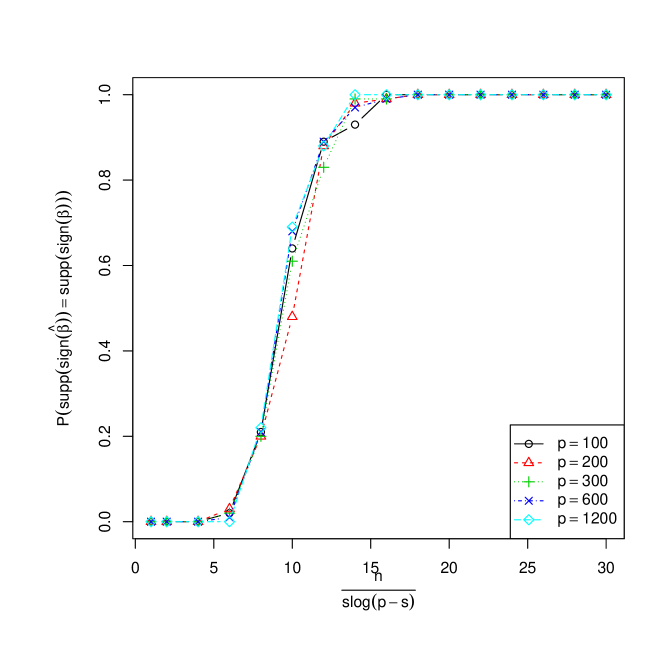
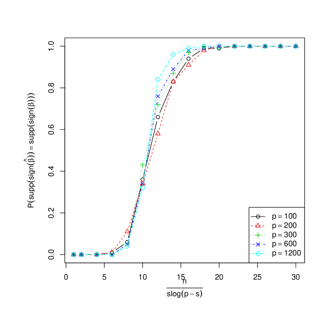
Appendix C Extra Numerical Studies Figures

Figure 4: Efficiency Curves for DT-SIR, s=logp,Γ=nslog(ps)[0,30]formulae-sequence𝑠𝑝Γ𝑛𝑠𝑝𝑠030s=\log{p},~{}\Gamma=\frac{n}{s\log(p-s)}\in[0,30]
Refer to caption
(a) Model (13)
Refer to caption
(b) Model (14)
Refer to caption
(c) Model (15)
Refer to caption
(d) Model (16)
Figure 5: Efficiency Curves for SDP, s=logp,Γ=nslog(ps)[0,40]formulae-sequence𝑠𝑝Γ𝑛𝑠𝑝𝑠040s=\log{p},~{}\Gamma=\frac{n}{s\log(p-s)}\in[0,40]
Refer to caption
(a) Model (13)
Refer to caption
(b) Model (14)
Refer to caption
(c) Model (15)
Refer to caption
(d) Model (16)
Figure 6: Efficiency Curves for DT-SIR, s=p,Γ=nslog(ps)[0,30]formulae-sequence𝑠𝑝Γ𝑛𝑠𝑝𝑠030s=\sqrt{p},~{}\Gamma=\frac{n}{s\log(p-s)}\in[0,30], 𝜷=𝜷~/𝜷~2𝜷~𝜷subscriptnorm~𝜷2\boldsymbol{\beta}=\widetilde{\boldsymbol{\beta}}/\|\widetilde{\boldsymbol{\beta}}\|_{2} according to (17)
Refer to caption
(a) Model (13)
Refer to caption
(b) Model (14)
Refer to caption
(c) Model (15)
Refer to caption
(d) Model (16)
Figure 7: Efficiency Curves for SDP, s=p,Γ=nslog(ps)[0,40]formulae-sequence𝑠𝑝Γ𝑛𝑠𝑝𝑠040s=\sqrt{p},~{}\Gamma=\frac{n}{s\log(p-s)}\in[0,40], 𝜷=𝜷~/𝜷~2𝜷~𝜷subscriptnorm~𝜷2\boldsymbol{\beta}=\widetilde{\boldsymbol{\beta}}/\|\widetilde{\boldsymbol{\beta}}\|_{2} according to (17)
Refer to caption
(a) Model (13)
Refer to caption
(b) Model (14)
Refer to caption
(c) Model (15)
Refer to caption
(d) Model (16)