Efficient Multiscale Gaussian Process Regression using Hierarchical Clustering

Abstract

Standard Gaussian Process (GP) regression, a powerful machine learning tool, is computationally expensive when it is applied to large datasets, and potentially inaccurate when data points are sparsely distributed in a high-dimensional feature space. To address these challenges, a new multiscale, sparsified GP algorithm is formulated, with the goal of application to large scientific computing datasets. In this approach, the data is partitioned into clusters and the cluster centers are used to define a reduced training set, resulting in an improvement over standard GPs in terms of training and evaluation costs. Further, a hierarchical technique is used to adaptively map the local covariance representation to the underlying sparsity of the feature space, leading to improved prediction accuracy when the data distribution is highly non-uniform. A theoretical investigation of the computational complexity of the algorithm is presented. The efficacy of this method is then demonstrated on smooth and discontinuous analytical functions and on data from a direct numerical simulation of turbulent combustion.

1 Introduction

The rapid growth in computing power has resulted in the generation of massive amounts of highly-resolved datasets in many fields of science and engineering. Against this backdrop, machine learning (ML) is becoming a widely-used tool in the identification of patterns and functional relationships that has resulted in improved understanding of underlying physical phenomena mjolsness2001 , characterization and improvement of models yairi1992 ; ling2015 ; eric2015 , control of complex systems gautier2015 , etc. In this work, we are interested in further developing Gaussian Process (GP) regression, which is a popular supervised learning technique. While GPs have been demonstrated to provide accurate predictions of the mean and variance of functional outputs, application to large-scale datasets in high-dimensional feature spaces remains a hurdle. This is because of the high computational costs and memory requirements during the training stage and the expense of computing the mean and variance during the prediction stage. To accurately represent high-dimensional function spaces, a large number of training data points must be used. In this work, an extension to GP regression is developed with the specific goal of applicability in noisy and large-scale scientific computing datasets.

The computational complexity of GPs at the training stage is related to the kernel inversion and the computation of the log-marginal likelihood. For example, an algorithm based on the Cholesky decomposition is one well-known approach chol . The computational complexity of Cholesky decomposition for a problem with $N$ training points is $O\left(N^{3}\right)$. For high-dimensional problems with large $N$, this can be prohibitive. Even if this cost can be reduced using, for instance, iterative methods gumerov-iter , the computation of the predictive mean and variance at $M$ test points will be $O\left(NM\right)$, and $O\left(N^{2}M\right)$, respectively. The evaluation (or testing) time could be of great significance if GP evaluations are made frequently during a computational process. Such a situation can occur in a scientific computing setting transprev ; eric2015 where GP evaluations may be performed every time-step or iteration of the solver. Reducing both the training and evaluation costs while preserving the prediction accuracy is the goal of the current work.

Much effort has been devoted to the construction of algorithms of reduced complexity. Among these is the family of methods of sparse Gaussian process regression. These methods seek to strategically reduce the size of the training set or find appropriate sparse representations of the correlation matrix through the use of induced variables. The covariance matrix, $\mathbf{\Phi}\in\mathbb{R}^{N\times N}$, contains the pairwise covariances between the $N$ training points. Descriptions for several methods of this family are provided by Quiñonero-Candela et al. quinonero2005 , who define induced variables $\mathbf{U}\in\mathbb{R}^{d\times P}$, $\mathbf{V}\in\mathbb{R}^{P}$ such that the prediction of a function $f(\mathbf{q})$ is given by

$$p(f|\mathbf{U})\sim\mathcal{N}(\underline{\phi}_{u}^{T}\mathbf{\Phi}_{u}^{-1}\mathbf{V},1+\sigma^{2}-\underline{\phi}_{u}^{T}\mathbf{\Phi}_{u}^{-1}\underline{\phi}_{u}),$$ (1)

where $\underline{\phi}_{u}\in\mathbb{R}^{P}$ is a vector whose elements are $\phi(\mathbf{u}_{i},\mathbf{q})$, and $\mathbf{\Phi}_{u}(m,n)=\phi(\mathbf{u}_{m},\mathbf{u}_{n})$. $P$ is the number of induced variables used in this representation, and $d$ is the dimensionality of the inputs; i.e. $\mathbf{u}$, $\mathbf{q}\in\mathbb{R}^{d}$. $\mathbf{q}$ is a single test input vector, and $\mathbf{u}_{m}$ is the $m$’th column of $\mathbf{U}$. $\phi$ is the covariance function. From this, it is evident that if $P<N$, the matrix inversion will be less costly to perform.

The process of determining the induced variables that can optimally represent the training set can introduce additional computational costs. The most basic method is to randomly select a fraction of data points and define them as the new training set, i.e. choosing $(\mathbf{U},\mathbf{V})$ from $(\mathbf{Q},\mathbf{y})$, where $\mathbf{Q}\in\mathbb{R}^{d\times N}$ and $\mathbf{y}\in\mathbb{R}^{N}$ are the original training inputs and outputs. Seeger et al. seeger2003 , Smola et al. smola2001 , and others have developed selection methods that provide better test results compared to random selection. In particular, Walder et al. walder2008 have extended the concept to include the ability to vary $\phi$ such that its hyperparameters are unique to each $\mathbf{u}$, i.e. $\phi=\phi_{i}(\mathbf{u}_{i},\mathbf{q})$. These methods often depend on optimizing modified likelihoods based on $(\mathbf{U},\mathbf{V})$, or on approximating the true log marginal likelihood titsias2009 . Methods that introduce new induced variables instead of using a subset of the training points can involve solving optimization problems, again requiring the user to consider the additional computational burden.

In addition to choosing the inducing variables, one may also change the form of the covariance function from $\phi$ to $\phi^{\prime}$, where

$$\phi^{\prime}(\mathbf{q}_{m},\mathbf{q}_{n})=\phi(\mathbf{q}_{m},\mathbf{U})\mathbf{\Phi}_{u}^{-1}\phi(\mathbf{q}_{n},\mathbf{U})^{T}.$$ (2)

In contrast to the case where only a subset of the training data is used, all training points are considered in this approach and the matrices are only of rank $P$. There are many variations on this type of manipulation of the covariance. Alternatively, one can approximate $\mathbf{\Phi}$ directly by obtaining random samples of the kernel, as is described by Rahimi et al. recht2007 . However, altering the covariance matrix can cause undesirable behaviors when computing the test variance, since some matrices no longer mathematically correspond to a Gaussian process. The work of Ambikasaran et al. ambikasaran improves the speed of GP regression through the hierarchical factorization of the dense covariance matrix into block matrices, resulting in a less costly inversion process.

Other methods of accelerating GP regression focus on dividing the training set into smaller sets of more manageable size. Snelson and Ghahramani snelson2007local employ a local GP consisting of points in the neighborhood of the test point in addition to a simplified global estimate to improve test results. In a similar fashion, the work of Park and Choi park2010 also takes this hierarchical approach, with the global-level GP informing the mean of the local GP. Urtasun and Darrell urtasun2008 use the local GP directly, without the induced variables. However, this requires the test points to be either assigned to a pre-computed neighborhood of training points snelson2007local , or to be determined on-line urtasun2008 . Both of these approaches to defining the neighbourhood can be quite expensive depending on training set size, though massive parallelization may mitigate the cost in some aspects keane2002 weiss2014 .

In this work, the data is partitioned into clusters based on modified k-center algorithms and the cluster centers are used to define a reduced training set. This leads to an improvement over standard GPs in terms of training and testing costs. This technique also adapts the covariance function to the sparsity of a given neighborhood of training points. The new technique will be referred to as Multiscale GP and abbreviated as MGP. Similar to the work of Snelson and Ghahramani snelson2007local , this flexibility may allow MGP to produce more accurate outputs by means of a more informed perspective on the input space. The sparse GP technique of Walder et al. walder2008 can been seen as a very general interpretation of our approach, though a key difference is that the points within the reduced training set originate entirely from the original training set, whereas  walder2008 computes new induced variables. Further, in our work, hyperparameters are restricted by the explicit choice and hierarchy of scales in order to streamline the process of their optimization. The work of Zhou et al. zhou2006 also employs multiple scales of covariance functions, but it does not take into account the neighbourhoods of training points, and neither does it seek to reduce the size of the training set.

The next section of this paper recapitulates the main aspects of standard GP regression. Section 3 introduces the philosophy behind the proposed approach and presents the algorithm. Section 4 analyses the complexity of the MGP algorithm for both testing and training. In section 5, quantitative demonstrations are presented on a simple analytical problems as well as on data derived from numerical simulations of turbulent combustion. Following this, key contributions are summarized.

2 Preliminaries of GP regression

In this section, a brief review of standard GP regression is presented. While a detailed review can be found in the excellent book by Rasmussen rbfgp2 , the description and notations below provide the necessary context for the development of the multiscale algorithm proposed in this paper.

We consider the finite dimensional weight-space view and the infinite dimensional function-space view as in Rasmussen rbfgp2 . Given a training set $\mathcal{D}$ of $N$ observations, $\mathcal{D}=\left\{\left(\mathbf{q}_{n},y_{n}\right)~{}|~{}n=1,...,N\right\}$, where $\mathbf{q}_{n}\in\mathbb{R}^{d}$ is an input vector and $y$ is a scalar output, the goal is to obtain the predictive mean, $m_{\ast}$, and variance, $v_{\ast}$, at an arbitrary test point $\mathbf{q}_{\ast}\in\mathbb{R}^{d}$. Training inputs are collected in the design matrix $Q\in\mathbb{R}^{d\times N}$, and the outputs form the vector $\mathbf{y\in}$ $\mathbb{R}^{N}$. Furthermore, it is assumed that

$$y=f\left(\mathbf{q}\right)+\epsilon,\quad\epsilon\sim\mathcal{N}(0,\sigma^{2}),$$ (3)

where $\epsilon$ is Gaussian noise with zero mean and variance $\sigma^{2}$.

For low dimensionality $d$ of the inputs, linear regression cannot satisfy a variety of dependencies encountered in practice. Therefore, the input is mapped into a high-dimensional feature space $\mathbb{R}^{D},$ $D>d$, and the linear regression model is applied in this space. To avoid any confusion with the original feature space $\mathbb{R}^{d}$, this space will be referred to as the “extended feature space” and its dimensionality can be referred to as the “size” of the system. Denoting the mapping function $\mathbf{\phi}\left(\mathbf{q}\right)$, $\mathbf{\phi}:\mathbb{R}^{d}\rightarrow\mathbb{R}^{D}$ we have

$$f\left(\mathbf{q}\right)=\mathbf{\phi}\left(\mathbf{q}\right)^{T}\mathbf{w=}\sum_{j=1}^{D}w_{j}\phi_{j}\left(\mathbf{q}\right)\mathbf{,\quad w}=\left(w_{1},...,w_{D}\right)\in\mathbb{R}^{D}.$$ (4)

The predictive mean and the covariance matrix can then be computed as

$$\overline{\mathbf{w}}=\frac{1}{\sigma^{2}}\Sigma\Phi\mathbf{y,\quad}\Sigma^{-1}=\frac{1}{\sigma^{2}}\Phi\Phi^{T}+\Sigma_{p}^{-1}.$$ (5)

The Bayesian formalism provides Gaussian distributions for the training outputs and for the predictive mean $m_{\ast}$ and variance $v_{\ast}$.

$$\mathbf{y} \sim \mathcal{N}(0,\Sigma_{l}),\quad y_{\ast}\sim\mathcal{N}(m_{\ast},v_{\ast}),$$ (6)

$$\Sigma_{l}^{-1} = \frac{1}{\sigma^{2}}\left(I-\frac{1}{\sigma^{2}}\Phi^{T}\Sigma\Phi\right),$$

$$m_{\ast} = \mathbf{\phi}\left(\mathbf{q}_{\ast}\right)^{T}\overline{\mathbf{w}},\quad v_{\ast}=\mathbf{\phi}\left(\mathbf{q}_{\ast}\right)^{T}\Sigma\mathbf{\phi}\left(\mathbf{q}_{\ast}\right)+\sigma^{2},$$ (7)

where $I$ is the identity matrix. These expressions allow for the computation of the log-marginal likelihood (LML),

$$\log p\left(\mathbf{y}|Q\right)=-\frac{1}{2}\mathbf{y}^{T}\Sigma_{l}^{-1}\mathbf{y}-\frac{1}{2}\log\left|\Sigma_{l}\right|-\frac{N}{2}\log\left(2\pi\right).$$ (8)

Maximization of this function leads to optimal values of hyper-parameters such as $\sigma^{2}$ and other variables that define $\mathbf{\phi}\left(\mathbf{q}\right)$.

3 Multiscale sparse GP regression

As stated earlier, the goal of the proposed GP-based regression process is to decrease the complexity of both training and testing and to make the prediction more robust for datasets that have a highly irregular distribution of features.

We consider Gaussian basis functions,

$$\phi_{j}\left(\mathbf{q}\right)=g\left(\mathbf{q},\mathbf{q}_{j}^{\prime},h_{j}\right)=\exp\left(-\frac{\left\|\mathbf{q-q}_{j}^{\prime}\right\|^{2}}{h_{j}^{2}}\right),\quad j=1,...,D,\quad\mathbf{\phi}=\left(\phi_{1},...,\phi_{D}\right)^{T},$$ (9)

where each function is characterized not only by its center $\mathbf{q}_{j}$, but now also by a scale $h_{j}$. The need for multiple scales may arise from the underlying physics (e.g. particle density estimation) or from the substantial non-uniformity of the input data distribution, which could, for instance, demand smaller scales in denser regions. Note that the matrix $\Phi\Phi^{T}$ in Eq. (5) is given by

$$\left(\Phi\Phi^{T}\right)_{ij} = \sum_{n=1}^{N}\phi_{i}\left(\mathbf{q}_{n}\right)\phi_{j}\left(\mathbf{q}_{n}\right)$$

$$= \sum_{n=1}^{N}\exp\left(-\frac{\left\|\mathbf{q}_{n}-\mathbf{q}_{i}^{\prime}\right\|^{2}}{h_{i}^{2}}-\frac{\left\|\mathbf{q}_{n}-\mathbf{q}_{j}^{\prime}\right\|^{2}}{h_{j}^{2}}\right),\quad i,j=1,...,D,$$

3.1 Sparse representations

While $N$ training points may be available and maximum information can be obtained when the size of the extended feature space $D=N$, we will search for subsets of these points leading to a lower size $D<N$. The size of the extended feature space is related to the accuracy of the low-rank approximation of matrix $\Phi$ built on the entire training set (i.e. for the case $D=N$).

Assume for a moment that we have a single scale, $h_{1}=...=h_{N}=h.$ If $h$ is chosen to be smaller than the minimum distance between the training points, the matrix $\Phi$ will have a low condition number and a low marginal likelihood. On the other end, if $h$ is substantially larger than the maximum distance between the training points the problem will be ill-posed and the marginal likelihood will be also low. The optima should lie between these extremes. If the solution is not sensitive to the removal of a few training points, a good low-rank approximation can be sought.

The fact that the $N\times N$ matrix $\Phi$ can be well-approximated with a matrix of rank $r<N$ means that $N-r$ rows or columns of this matrix can be expressed as a linear combination of the other rows or columns with relatively small error $\epsilon^{\prime}$. Assuming that $r$ locations (or centers) of the radial basis functions (or Gaussians) are given and denoting such centers by $\mathbf{q}_{j}^{\prime}$, $j=1,...,r$, we have

$$\phi_{n}\left(\mathbf{q}\right)=g\left(\mathbf{q},\mathbf{q}_{n},h_{n}\right)=\sum_{j=1}^{r}\eta_{nj}\phi_{j}\left(\mathbf{q}\right)+\epsilon_{n}^{\prime},\quad\mathbf{q}_{j}^{/}\in\mathbb{Q}^{\prime}\mathbb{\subset Q}\text{,\quad}n=1,...,N,$$ (11)

where $\eta_{nj}$ are coefficients to be determined. Hence, output (Eqn. 3), where $f$ is expanded as Eqn. 4 with $D=N$, can be written as

$$y\left(\mathbf{q}\right) = \sum_{n=1}^{N}w_{n}\phi_{n}\left(\mathbf{q}\right)+\epsilon=\sum_{j=1}^{r}w_{j}^{\prime}\phi_{j}\left(\mathbf{q}\right)+\epsilon+\epsilon^{\prime}\mathbf{,}$$ (12)

$$w_{j}^{\prime} = \sum_{n=1}^{N}w_{n}\eta_{nj},\quad\epsilon^{\prime}=\sum_{n=1}^{N}w_{n}\epsilon_{n}^{\prime}.$$

This shows that if $\epsilon^{\prime}$ is lower or comparable with noise $\epsilon$, then a reduced basis can be used and one can simply set the size of the extended feature space to be the rank of the low-rank approximation, $D=r$, and coefficients $w_{j}^{\prime}$ can be determined by solving a $D\times D$ system instead of an $N\times N$ system.

3.2 Representative training subsets

Let us consider now the problem of determination of the centers of the basis functions and scales $h_{j}$. If each data-point is assigned a different scale, then the optimization problem will become unwieldy, as $D$ hyperparameters will have to be determined. Some compromises are made, and we instead use a set of scales $h_{1},...,h_{S}$. In the limit of $S=1$, we have a single scale model, while at $S=D$ we prescribe a scale to each training point. To reduce the number of scales while providing a broad spectrum of scales, we propose the use of hierarchical scales, e.g. $h_{s}=h_{1}\beta^{s-1}$, $s=1,...,S$, where $h_{1}$ is of the order of the size of the computational domain and $\beta<1$ is some dimensionless parameter controlling the scale reduction.

While there exist several randomization-based strategies to obtain a low-rank representation by choosing $D$ representative input points quinonero2005 , we propose a more regular, structured approach. For a given scale $h$, we can specify some distance $a=\gamma h$, where $\gamma<1$ is chosen such that

• The distance from any input point to a basis point is less than $a$. Such a construction provides an approximately uniform coverage of the entire training set with $d$-dimensional balls of radius $a$.

• The number of such balls is - in some sense - optimal. Note that smaller $\gamma$ results in smaller errors $\epsilon_{n}^{\prime}$ and $\epsilon^{\prime}$ and larger $r$ in Eqs. (11) and (12). If $\gamma<h/a_{\min}$, where $a_{\min}$ is the minimal distance between the points in the training set, then $\epsilon^{\prime}=0$ and $r=D=N$, which corresponds to a full rank representation.

The problem of constructing an optimal set as described above is computationally NP-hard. However, approximate solutions can be obtained with a modification of the well-known $k$-means algorithm kmeans . In computational geometry problems, the $k$-means algorithm partitions a domain in $d$-dimensional space into a prescribed number, $k$, of clusters. In the present problem, the number of clusters is unknown, but the distance parameter $a$ is prescribed. Thus, the number of centers depends on the input point distribution and can be determined after the algorithm is executed. Since only the cluster centers are required for the present problem, the following algorithm is used:

Algorithm #1: Determination of cluster centers and k Input: set of training points $\mathbb{Q=}\left\{\mathbf{q}_{1},...,\mathbf{q}_{N}\right\}$, max cluster radius $a$. 1. Define $\mathbb{R}_{0}=\mathbb{Q}$ and set $k=0$; 2. Do steps 3 to 6 while $\mathbb{R}_{k}\neq\emptyset;$ 3. $k=k+1;$ 4. Assign $\mathbf{q}_{k}^{\prime}=\mathbf{q}_{j}\in$ $\mathbb{R}_{k-1}$ (where $\mathbf{q}_{j}$ is a random point from set $\mathbb{R}_{k-1}$) 5. Find all points $\mathbf{q}_{ki}\in\mathbb{R}_{k-1}$, such that $\left|\mathbf{q}_{ki}-\mathbf{q}_{k}^{\prime}\right|\leqslant a$. 6. Define $\mathbb{Q}_{k}=\left\{\mathbf{q}_{ki}\right\}$ and $\mathbb{R}_{k}=\mathbb{R}_{k-1}\backslash\mathbb{Q}_{k}$. Output: set of cluster centers $\mathbb{Q}^{\prime}\mathbb{=}\left\{\mathbf{q}_{1}^{\prime},...,\mathbf{q}_{k}^{\prime}\right\}$, number of clusters $k$.

The construction of training subsets in the case of multiple scales requires further modification of the algorithm. Starting with the coarsest scale $h_{1}$, $k_{1}$ centers can be determined using Algorithm 1 with distance parameter $a_{1}=\gamma h_{1}$. In our approach, we select the bases such that each input point can serve as a center of only one basis function; therefore, the $k_{1}$ cluster centers of scale $h_{1}$ should be removed from the initial training set to proceed further. Next, we partition the remaining set using Algorithm 1 with distance parameter $a_{2}=\gamma h_{2}$ and determine $k_{2}$ cluster centers. After removal of these points we repeat the process until scale $h_{S}$ is reached at which we determine $k_{S}$ cluster centers and stop the process. This algorithm is described below.

Algorithm #2: Determination of cluster centers in multiple scales Input: Set of training points $\mathbb{Q}=\left\{\mathbf{q}_{1},...,\mathbf{q}_{N}\right\}$, set of scales $\mathbb{H=}\left\{h_{1},...,h_{S}\right\}$, parameter $\gamma$. 1. Define $\mathbb{R=Q};$ 2. Do steps 3 to 4 for $s=1,...,S;$ 3. Execute Algorithm #1 with input $\mathbb{R}$ and max cluster radius $a=\gamma h_{s}$ and get cluster centers $\mathbb{Q}_{s}^{\prime}$ and number of clusters $k_{s};$ 4. Set $\mathbb{R=R}\backslash\mathbb{Q}_{s}^{\prime}.$ Output: set of cluster centers $\mathbb{Q}^{\prime}=\mathbb{\cup Q}_{s}^{\prime}$, $\mathbb{Q}_{s}^{\prime}=\left\{\mathbf{q}_{1}^{(s)\prime},...,\mathbf{q}_{k_{s}}^{(s)\prime}\right\}$, number of clusters for each scale $k_{s}$, $s=1,...,S$.

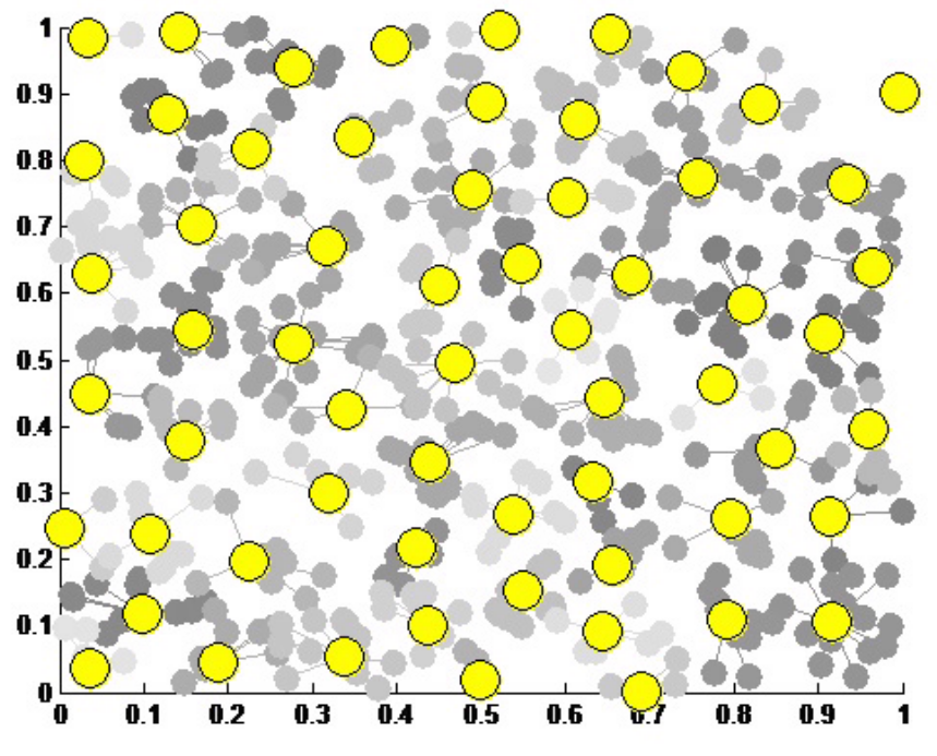
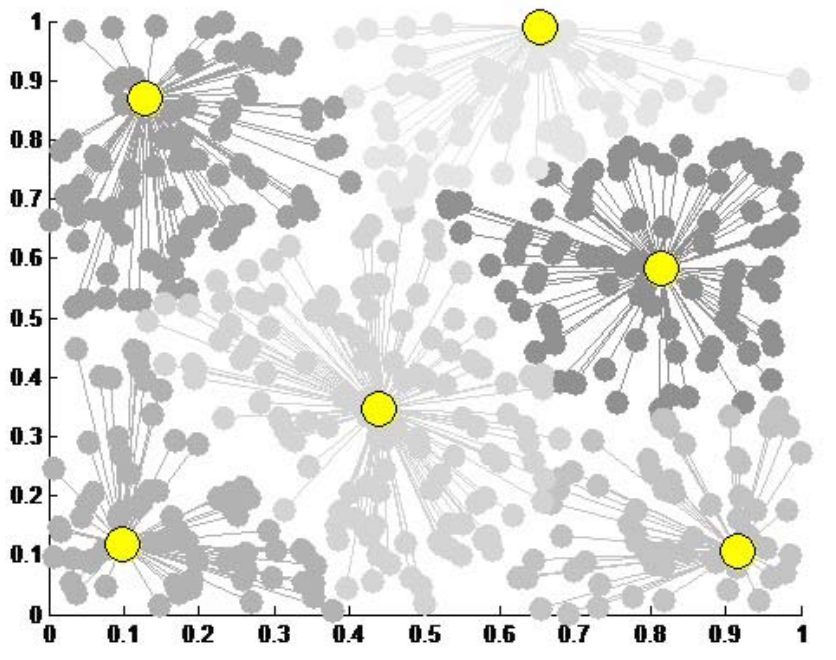
Figure 1: The separation of 500 random points distributed inside a unit square into clusters. The cluster centers are shown in yellow; points belonging to different clusters are in different shades of gray. Left: small $h_{n}$. Right: large $h_{n}$.

Figure 1 illustrates the clustering of a 2-dimensional dataset. In principle, one can use the process even further until all the points in the training set become the cluster centers at some scale (i.e. $D=N$). However, as mentioned above, the reduction of the basis, $D<N$, is important to reduce the computational complexity of the overall problem.

4 Complexity

The asymptotic complexity of algorithm #1 is $O\left(Nk\right)$ and that of algorithm #2 is $O\left(ND\right)$. While fast neighbor search methods cheng1984 can accelerate these algorithms, the overall computational cost of the regression is still expected to be dominated by the training and evaluation costs. It is thus instructive to discuss the complexities of different algorithms available for training and testing, especially when $D\ll N$.

4.1 Training

The goal of the training stage is to determine quantities necessary for computations in the testing stage. At this point, two types of computations should be recognized: i) pre-computations, when the set of hyperparameters is given, and ii) the optimization problem to determine the hyperparameters.

To accomplish the first task, we use the following steps:

• The initial step is to form the matrix $\Phi$, and then the $D\times D$ matrix $\Sigma^{-1}$ in Eq. (5). According to Eq. (3), the cost of this step is $O\left(ND^{2}\right)$. Note that this cost is much larger than the $O\left(ND\right)$ required to determine the basis function centers using the $k$-means type algorithm described in Section 3.2.

• The next step involves the determination of the weights $\overline{\mathbf{w}}$ from Eq. (5) This requires solving a $D\times D$. If solutions are obtained through direct methods, the cost is $O\left(D^{3}+ND\right)$.

• Following this, the inverse $\Sigma$ should be determined. The Cholesky decomposition is typically used in this situation rbfgp2 ;

  $$\Sigma^{-1}=L_{D}L_{D}^{T},$$ (13)

  where $L_{D}$ is the lower triangular matrices. The decompositions can be performed with cost $O\left(D^{3}\right)$, respectively. Note that the Cholesky decompositions can also be used to solve the systems for $\overline{\mathbf{w}}$, in which case the complexity of solution becomes $O\left(D^{2}+ND\right)$.

The second task requires the computation of the log marginal likelihood. If one uses Eq. (8) directly then the task becomes computationally very expensive (complexity $O\left(N^{3}\right)$). The complexity can be reduced with the aid of the following lemma.

Lemma 1

Determinants of matrices $\Sigma$ and $\Sigma_{l}$, defined by Eqs. (5) and (6), are related as

$$\frac{1}{\sigma^{2N}}\frac{\left|\Sigma\right|}{\left|\Sigma_{p}\right|}=\frac{1}{\left|\Sigma_{l}\right|}.$$ (14)

Proof

According to the definition of $\Sigma_{l}$ (6), we have in the right hand side of Eq. (14)

$$\frac{1}{\left|\Sigma_{l}\right|}=\left|\Sigma_{l}^{-1}\right|=\frac{1}{\sigma^{2N}}\left|I-\frac{1}{\sigma^{2}}\Phi^{T}\Sigma\Phi\right|.$$ (15)

Note now the Sylvester determinant theorem, which states that

$$\left|I_{N}+AB\right|=\left|I_{D}+BA\right|,$$ (16)

where $A$ is an $N\times D$ matrix and $B$ is $D\times N$, while $I_{N}$ and $I_{D}$ are the $N\times N$ and $D\times D$ identity matrices. Thus, we have in our case

$$\left|I-\frac{1}{\sigma^{2}}\Phi^{T}\Sigma\Phi\right|=\left|I_{N}-\frac{1}{\sigma^{2}}\Phi^{T}\left(\Sigma\Phi\right)\right|=\left|I_{D}-\frac{1}{\sigma^{2}}\left(\Sigma\Phi\right)\Phi^{T}\right|=\left|I-\frac{1}{\sigma^{2}}\Sigma\Phi\Phi^{T}\right|.$$ (17)

From Eq. (5) we have

$$I = \Sigma\Sigma^{-1}=\Sigma\left(\frac{1}{\sigma^{2}}\Phi\Phi^{T}+\Sigma_{p}^{-1}\right),$$ (18)

$$\left|I-\frac{1}{\sigma^{2}}\Sigma\Phi\Phi^{T}\right| = \left|\Sigma\Sigma_{p}^{-1}\right|=\frac{\left|\Sigma\right|}{\left|\Sigma_{p}\right|}.$$

Combining results (15), (17), and (18), one can see that Eq. (14) holds.

Now, replacing $\Sigma_{l}^{-1}\mathbf{y}$ in the first term in the right-hand side of Eq. (8) with expressions for $\Sigma_{l}^{-1}$ and $\overline{\mathbf{w}}$ from Eqs. (5) and (6) and using Eq. (14) in the second term, we obtain

$$\log p\left(\mathbf{y}|X\right)=-\frac{1}{2\sigma^{2}}\left(\mathbf{y}-\Phi^{T}\overline{\mathbf{w}}\right)^{T}\mathbf{y}-\frac{1}{2}\log\left|\Sigma^{-1}\right|-\frac{1}{2}\log\left|\Sigma_{p}\right|-\frac{N}{2}\log\left(2\pi\sigma^{2}\right).$$ (19)

In the case of $\Sigma_{p}=\sigma_{p}^{2}I$ and using the Cholesky decomposition of $\Sigma^{-1}$, we obtain

$$\log p\left(\mathbf{y}|X\right)=-\frac{1}{2\sigma^{2}}\left(\mathbf{y}-\Phi^{T}\overline{\mathbf{w}}\right)^{T}\mathbf{y}-\sum_{j=1}^{D}\log L_{D,jj}-\frac{N}{2}\log\left(2\pi\sigma_{p}^{2}\sigma^{2}\right).$$ (20)

Here, the cost of computing the first term on the right hand side is $O\left(ND\right)$, and the cost of the second term is $O\left(D\right)$.

Multi-dimensional optimization is usually an iterative process. Assuming that the number of iterations is $N_{iter}$, we can write the costs of the training steps marked by the respective superscripts as follows

$$C_{train}=O\left(N_{iter}D\left(N+D^{2}\right)\right)\text{.}$$ (21)

4.2 Testing

The cost of testing can be estimated from Eq. (6) as the cost of computing the predictive mean and variance. Taking into account the Cholesky decomposition (13), these costs can be written as

$$C_{mean}=O\left(MD\right)\text{,\quad}C_{var}=O\left(MD^{2}\right)\text{.}$$ (22)

where $M$ is the number of test points. The cost for computing the variance is much higher than the cost for computing the mean, because it is determined by the cost of solving triangular systems of size $D\times D$ per evaluation point.

5 Numerical Results

In this section, a set of simple analytical examples are first formulated to critically evaluate the accuracy and effectiveness of MGP and to contrast its performance with conventional GP regression. Following this, data from a turbulent combustion simulation is used to assess the viability of the approach in scientific computing problems.

5.1 Analytical examples

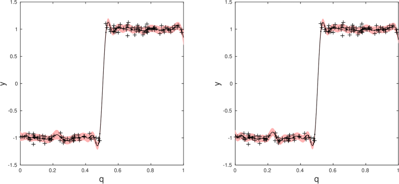
Figure 2: Comparison of the output of the standard kernel GP using a Gaussian kernel (left) and MGP with $S=1$ (right) for a step function. The crosses are training points ($N=128$), while the continuous lines and shaded areas show the predictive mean and the variance.

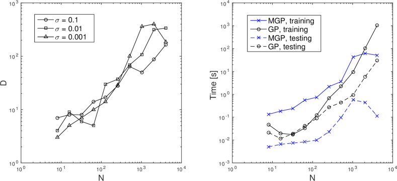
Figure 3: Comparison of the performance of the standard GP and MGP for the step function in Figure 2. The plot on the left shows the size of the extended feature space for different input noise $\sigma$. The wall clock time is obtained using MATLAB on a typical desktop PC.

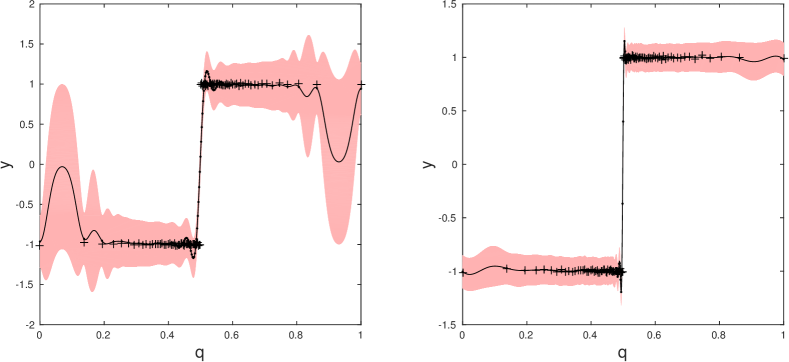
Figure 4: Comparison of the standard GP (left) and MGP (right) for a step function. In contrast to Figure 2, the training point distribution is non-uniform with an exponential density increase near the jump. The number of training points $N=101$. Gaussian noise with $\sigma=0.03$ was added. The crosses represent training points, while the continuous lines and shaded areas show the predictive mean and the variance. The dots on the continuous line have abscissas of the training points.

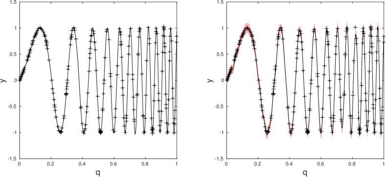
Figure 5: Comparison of performance of the standard GP (left) and MGP with $S=1$ (right) for a sine function, $y=\sin(2\pi q(4q+1)^{1.5})$ with Gaussian noise of standard deviation $\sigma=0.01$. Crosses represent training points ($N=128$); continuous lines and shaded regions show the predictive mean and the variance.

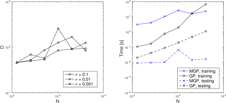
Figure 6: Comparison of the performance of the standard GP and MGP for the sine function in Figure 5. The wall-clock time is obtained using MATLAB on a typical desktop PC.

The first numerical example we present is a 1-D step function ($d=1$). We compare the standard kernel GP with a Gaussian kernel and the present MGP algorithm restricted to a single scale ($S=1$). The training set of size $N$ was randomly selected from 10000 points distributed in a uniform grid. Points not used for training were used as test points. The initial data was generated by adding normally distributed noise with standard deviation $\sigma$ to the step function. Optimal hyperparameters were found using the Lagarias algorithm for the Nelder-Mead method (as implemented by MATLAB’s fminsearch function) lagarias . For the standard GP, $\sigma$ and $h$ were optimized, while for the MGP algorithm, the optimal $\gamma$ was determined in addition to $\sigma$ and $h$. In both cases, the optimal $\sigma$ was close to the actual $\sigma$ used for data generation. The ratio between the optimal $h$ for the kernel and the finite-dimensional (“weight-space”) approaches was found to be approximately $1.4$, which is consistent with the difference of $\sqrt{2}$ predicted by the theory (the distinction between the weight space and function space approaches is provided in Ref. rbfgp2 ).

The plots in Figure 2 show that there is no substantial difference in the mean and the variance computed using both methods, while the sparse algorithm required only $D=38$ functions compared to the $N=128$ required for the standard method. Figure 3 shows the relationship between the extended feature space (D) with respect to the size of the training set (N). Ideally, this should be a linear dependence, since the step function is scale-independent. Due to random noise and the possibility that the optimization may converge to local minima of the objective function, however, the relationship is not exactly linear. Since $D$ is nevertheless several times smaller than $N$, the wall-clock time for the present algorithm is shorter than that for the standard GP in both testing and training, per optimizer iteration. The total training time for the present algorithm can be larger than that of the standard algorithm due to the overhead associated with the larger number of hyperparameters and the resultant increase in the number of optimization iterations required. However, we observed this only for relatively small values of $N$. For larger $N$, such as $N=4096$, the present algorithm was approximately 5, 10, and 20 times faster than the standard algorithm for $\sigma=0.1$, $0.01$, and $0.001$, respectively.

Figure 4 illustrates a case where the training points are distributed non-uniformly. Such situations frequently appear in practical problems, where regions of high functional gradients are sampled with higher density to provide a good representation of the function. For example, adaptive meshes to capture phenomena such as shockwaves and boundary layers in fluid flow fall in this category. In the case illustrated here, the training points were distributed with exponential density near the jump ($q=0.5\pm h_{t}\ln z$, $\exp\left(-0.5/h_{t}\right)\leqslant z\leqslant 1$, where $z$ are distributed uniformly at the nodes of a regular grid. $h_{t}=0.1$ was used). For MGP, the number of scales was $S=6$ and the other hyperparameters were optimized using the same routine as before. Due to multiple extrema in the objective function, it is rather difficult to optimize the number of  scales, $S$. In practice, one should start from several initial guesses or fix some parameters such as $S$. We used several values of $S$ and observed almost no differences for $5\leq S\leq 10$, while results for $S=1$ and $S=2$ were substantially different from the cases where $S>2$.

It is seen that the MGP provides a much better fit of the step function in this case than the standard method. This is achieved due to its broad spectrum of scales. In the present example, we obtained the following optimal parameters for scales distributed as a geometric progression, $h_{s}=h_{1}\beta^{s-1}$: $h_{\max}=h_{1}=0.1233$, $h_{\min}=h_{6}=0.0032$, and $\beta=0.4806$. Other optimal parameters were $\gamma=0.258$ and $\sigma=0.127$. For the standard GP, the optimal scale was $h=0.0333$. Figure 4 shows that with only a single intermediate scale, it is impossible to approximate the function between training points with a large spacing, whereas MGP provides a much better approximation. Moreover, since $h_{\min}<h$, we also have a better approximation of the jump, i.e. of small-scale behavior. This is clearly visible in the figure; the jump for the standard GP is stretched over about 10 intervals between sampling points, while the jump for MGP only extends over 3 intervals. Note that in the present example, we obtained $D=N=101$, so the wall-clock time for testing is not faster than the standard GP. However, this case illustrates that multiple scales can provide good results for substantially non-uniform distributions where one scale description is not sufficient.

As final analytical example, we explore a sine wave with varying frequency, depicted in Figure 5. As before, $N$ training points are randomly chosen from a uniform distribution, and $M=10000-N$ test points are used. For MGP, $S=1$ was used. Compared to the previous examples, this is an intermediate case in terms of scale dependence. One noteworthy result from this dataset is that $D$ is almost constant with respect to $N$, as seen in Figure 6. This shows that when the function is relatively smooth, the optimization process is not limited to producing a linear relationship between $D$ and $N$. Another result is that the output variance of the multiscale method is visibly higher than that of the standard method. For the previous cases, the variances have been either been close to equal, or the standard method would produce the higher variance. This could be due to the fact that $h$ and $D$ are inherently related for the current method, whereas $h$ is unrestricted for the standard GP. Since $D<N$, the multiscale $h$ for $S=1$ is typically greater than the standard method’s $h$. According to Eq. (7), this would result in greater variance.

5.2 Data from Turbulent Combustion

Combustion in the presence of turbulent flow involves an enormous disparity in time and length scales, meaning that direct numerical simulations (DNS) are not possible in practical problems. Large eddy simulations (LES), in which the effect of scales smaller than the mesh resolution (i.e. subgrid scales) are modeled, is often a pragmatic choice. A key difficulty in LES of combustion is the modeling of the subgrid scale fluxes in the species transport equations kant1 ; kant2 . These terms arise as a result of the low-pass filtering - represented by the operator $(\bar{\cdot})$ - of the governing equations, and are of the form

$$f_{k}=\overline{\rho u_{k}C}-\frac{\overline{\rho u_{k}}\overline{\rho C}}{\bar{\rho}}$$ (23)

where $\rho,u,C$ represent density, velocity and species mass fraction, respectively. Subgrid-scale closures based on concepts from non-reacting flows, such as the equation below,

$$f_{k}=-\frac{\overline{\rho}C_{s}^{2}\Delta^{2}\sqrt{2\tilde{S}_{ij}\tilde{S}_{ij}}}{Sc}\frac{\partial\tilde{c}}{\partial x_{k}}$$ (24)

are found to be inadequate for turbulent combustion. Modeling of the scalar fluxes thus continues to be an active area of research, and many analytical models are being evaluated by the community. Reference  chakraborthy provides a concise summary of such developments in the area of premixed turbulent flames.

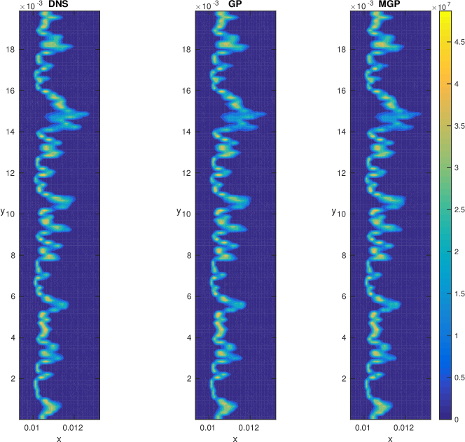
Figure 7: Contours of $F_{1}$ on the test $x-y$ plane. Left: DNS values (exact). Center: GP output. Right: MGP output.

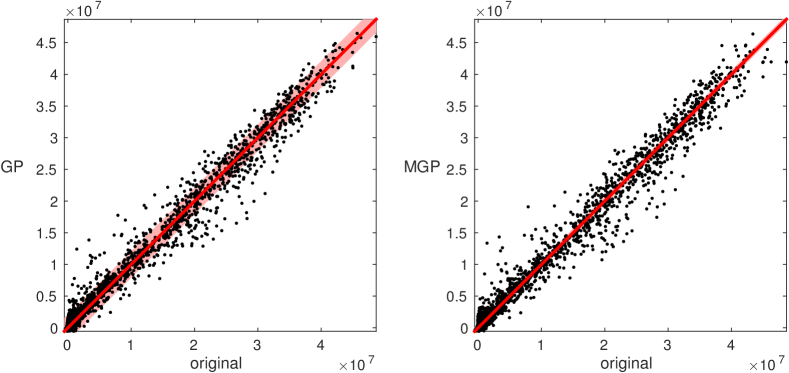
Figure 8: Original test output versus learned result for $F_{1}$. Red regions are $\pm\sigma$ from the diagonal, i.e. the optimized estimate of the input noise.

In this work, we intend to apply GP and MGP to identify the model relationships from data. The simulation data is obtained from Ref. raman , in which DNS of a propagating turbulent flame is performed. The configuration involves a premixed hydrogen-air flame propagating in the x-direction. The flame forms a thin front between the burnt and unburnt gases. Specifically, we attempt to learn the normalized flux in the x-direction, $F_{1}$, as a function of seven variables:

$$F_{1}=\frac{f_{1}}{\overline{\rho}\Delta^{2}}=f(\nabla\tilde{u},\nabla\tilde{c},\tilde{S})$$ (25)

A total of 3 million training points were generated from the dataset by performing low-pass filtering. Some care was taken in choosing training points. Since the flame is thin relative to the size of the domain, the majority of the data points were found to lie outside the region where $F_{1}$ is nonzero. To mitigate this disadvantageous distribution, 80 percent of the training points were randomly chosen from the data with $f_{1}>0.05$, and 20 percent were chosen from data with $f_{1}\leq 0.05$, i.e. outside the flame. 45000 training points were used in total. For testing, a single $x-y$ plane of around 6500 points was set aside.

The predictive results on this plane are shown in Table 1, and Figure 8 shows the ML output versus the true DNS values. From these plots, it is seen that MGP has achieved a fifty-fold increase in evaluation speed for a corresponding two percent increase in error. In the scatter plot, MGP appears to perform better than GP for low values of $F_{1}$ and worse for high values, but the overall difference is small. Figure 7 is a side-by-side comparison of contours of $F_{1}$ from DNS and from GP and MGP. It is especially evident in the contour plot that GP and MGP are both able to capture features of the flame, whereas analytical models described in Ref. chakraborthy were not as accurate. Figure 9 plots $F_{1}$ along several locations perpendicular ($x$) and parallel ($y$) to the flame in the test plane.

Table 1: Numerical results for learning $F_{1}$ in the flame. Error is defined as $||\mathbf{y}-f(\mathbf{Q}_{*})||/||\mathbf{y}||$, where $\mathbf{y}$ is a vector of the exact outputs $F_{1}$, and $f(\mathbf{Q}_{*})$ is a vector of the GP or MGP outputs at the test points $\mathbf{Q}_{*}$. Time is test time in seconds, obtained in MATLAB. MGP utilized 3 scales.

	GP		MGP
	Error	Time	Error	Time
$F_{1}$	0.1087	$4.2\times 10^{1}$	0.1105	$8.0\times 10^{-1}$

(a) $y=2\times 10^{-5}$

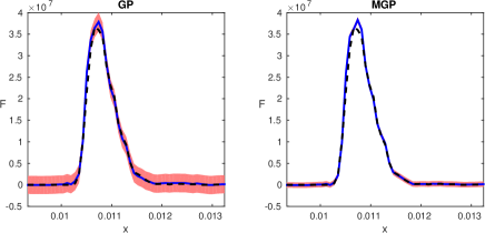
(b) $y=8\times 10^{-4}$

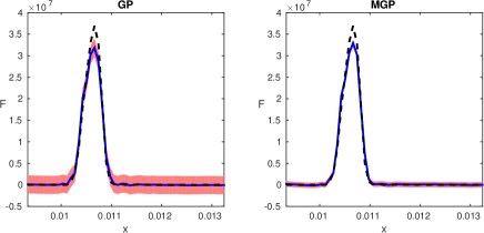
(c) $y=5\times 10^{-3}$

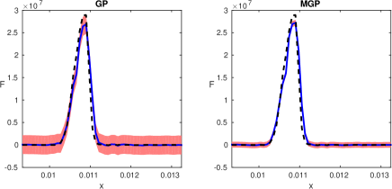
(d) $y=1\times 10^{-2}$

Figure 9: $F_{1}$ as a function of $x$ for four different constant values of $y$ on the test $x-y$ plane. Dashed black lines are from DNS. GP results on the left, MGP results on the right. Red regions are one standard deviation for the output.

6 Conclusion

In this paper, a new Gaussian process (GP) regression technique was presented. The method, referred to as MGP, introduces multiple scales among the Gaussian basis functions and employs hierarchical clustering to select centers for these sparse basis functions. These modifications reduce the computational complexity of GP regression and also achieve better accuracy than standard GP regression when training points are non-uniformly distributed in the $d$-dimensional feature space. We illustrated these improvements through analytical examples and in a turbulent combustion datasets.

In analytical examples with smooth functions, the MGP was shown to be at least an order of magnitude faster than the standard GP for a similar level of accuracy. In problems with discontinuities, the MGP is shown to provide a much better fit. In the turbulent combustion example in 7 dimensions, the MGP was shown to achieve a fifty-fold increase in evaluation speed for a corresponding two percent increase in error over the GP method. Overall, MGP is well-suited for regression problems where the inputs are unevenly distributed or where training and testing speeds are critical.

Based on the results presented in this work, MGP offers promise as a potentially attractive method for use in many scientific computing applications in which datasets may be large, and sparsely distributed in a high-dimensional feature space. The MGP can be especially useful when predictive evaluations are performed frequently. However, further developments and more detailed application studies are warranted. It was observed that the optimization process is more likely to terminate at local minima compared to conventional GPs. An immediate area of investigation could explore more efficient and robust techniques for optimization of the hyperparameters. Since an appealing feature of MGP is the reduced complexity when working with large datasets, efficient parallelization strategies should be explored.

The software and all the examples in this paper are openly available at http://umich.edu/~caslab/#software.

References

- (1) Mjolsness, E. and DeCoste, D., “Machine learning for science: state of the art and future prospects,” Science, Vol. 293, No. 5537, 2001, pp. 2051–2055.
- (2) Yairi, T., Kawahara, Y., Fujimaki, R., Sato, Y., and Machida, K., “Telemetry-mining: a machine learning approach to anomaly detection and fault diagnosis for space systems,” Space Mission Challenges for Information Technology, 2006. SMC-IT 2006. Second IEEE International Conference on, IEEE, 1992, pp. 8–pp.
- (3) Ling, J. and Templeton, J., “Evaluation of machine learning algorithms for prediction of regions of high Reynolds averaged Navier Stokes uncertainty,” Physics of Fluids, Vol. 27, No. 8, 2015.
- (4) Parish, E. and Duraisamy, K., “A Paradigm for data-driven predictive modeling using field inversion and machine learning,” Journal of Computational Physics, Vol. 305, 2016, pp. 758–774.
- (5) Gautier, N., Aider, J., Duriez, T., Noack, B. R., Segond, M., and Abel, M., “Closed-loop separation control using machine learning,” Journal of Fluid Mechanics, Vol. 770, 2015, pp. 442–457.
- (6) Wilkinson, J., The algebraic eigenvalue problem, Vol. 87, Clarendon Press Oxford, 1965.
- (7) Gumerov, N. A. and Duraiswami, R., “Fast radial basis function interpolation via preconditioned Krylov iteration,” SIAM Journal on Scientific Computing, Vol. 29, No. 5, 2007, pp. 1876–1899.
- (8) Duraisamy, K., Zhang, Z., and Singh, A., “New Approaches in Turbulence and Transition Modeling Using Data-driven Techniques,” 2014.
- (9) Quiñonero-Candela, J. and Rasmussen, C. E., “A unifying view of sparse approximate Gaussian process regression,” The Journal of Machine Learning Research, Vol. 6, 2005, pp. 1939–1959.
- (10) Seeger, M., Williams, C., and Lawrence, N., “Fast forward selection to speed up sparse Gaussian process regression,” Artificial Intelligence and Statistics 9, No. EPFL-CONF-161318, 2003.
- (11) Smola, A. J. and Bartlett, P., “Sparse Greedy Gaussian Process Regression,” Advances in Neural Information Processing Systems 13, MIT Press, 2001, pp. 619–625.
- (12) Walder, C., Kim, K. I., and Schölkopf, B., “Sparse multiscale Gaussian process regression,” Proceedings of the 25th International Conference on Machine learning, 2008, pp. 1112–1119.
- (13) Titsias, M. K., “Variational learning of inducing variables in sparse Gaussian processes,” International Conference on Artificial Intelligence and Statistics, 2009, pp. 567–574.
- (14) Rahimi, A. and Recht, B., “Random features for large-scale kernel machines,” Advances in neural information processing systems, 2007, pp. 1177–1184.
- (15) Ambikasaran, S., Foreman-Mackey, D., Greengard, L., Hogg, D., and O’Neil, M., “Fast Direct Methods for Gaussian Processes,” 2016.
- (16) Snelson, E. and Ghahramani, Z., “Local and global sparse Gaussian process approximations,” International Conference on Artificial Intelligence and Statistics, 2007, pp. 524–531.
- (17) Park, S. and Choi, S., “Hierarchical Gaussian Process Regression,” ACML, 2010, pp. 95–110.
- (18) Urtasun, R. and Darrell, T., “Sparse probabilistic regression for activity-independent human pose inference,” Computer Vision and Pattern Recognition, 2008. CVPR 2008. IEEE Conference on, IEEE, 2008, pp. 1–8.
- (19) Choudhury, A., Nair, P. B., and Keane, A. J., “A Data Parallel Approach for Large-Scale Gaussian Process Modeling.” SDM, SIAM, 2002, pp. 95–111.
- (20) Gramacy, R. B., Niemi, J., and Weiss, R. M., “Massively parallel approximate Gaussian process regression,” SIAM/ASA Journal on Uncertainty Quantification, Vol. 2, No. 1, 2014, pp. 564–584.
- (21) Zhou, Y., Zhang, T., and Li, X., “Multi-scale Gaussian Processes model,” Journal of Electronics (China), Vol. 23, No. 4, 2006, pp. 618–622.
- (22) Rasmussen, C. E., “Gaussian processes for machine learning,” 2006.
- (23) Hartigan, J. A. and Wong, M. A., “Algorithm AS 136: A k-means clustering algorithm,” Applied statistics, 1979, pp. 100–108.
- (24) Cheng, D., Gersho, A., Ramamurthi, B., and Shoham, Y., “Fast search algorithms for vector quantization and pattern matching,” Acoustics, Speech, and Signal Processing, IEEE International Conference on ICASSP’84., Vol. 9, IEEE, 1984, pp. 372–375.
- (25) Lagarias, J. C., Reeds, J. A., Wright, M. H., and Wright, P. E., “Convergence properties of the Nelder–Mead simplex method in low dimensions,” SIAM Journal on optimization, Vol. 9, No. 1, 1998, pp. 112–147.
- (26) Lipatnikov, A. N. and Chomiak, J., “Effects of premixed flames on turbulence and turbulent scalar transport,” Progress in Energy and Combustion Science, Vol. 36, No. 1, 2010, pp. 1–102.
- (27) Tullis, S. and Cant, R. S., “Scalar transport modeling in large eddy simulation of turbulent premixed flames,” Proceedings of the Combustion Institute, Vol. 29, No. 2, 2002, pp. 2097–2104.
- (28) Gao, Y., Klein, M., and Chakraborty, N., “Assessment of sub-grid scalar flux modelling in premixed flames for Large Eddy Simulations: A-priori Direct Numerical Simulation analysis,” European Journal of Mechanics - B/Fluids, Vol. 52, 2015, pp. 97 – 108.
- (29) Hassanaly, M., Raman, V., Koo, H., and Colkett, M. B., “Influence of Fuel Stratification on Turbulent Flame Propagation,” 2014.